Time memory effect in entropy decay
of Ornstein-Uhlenbeck operators

Abstract.

We investigate the effect of memory terms on the entropy decay of the solutions to equations with Ornstein-Uhlenbeck operators. Our assumptions on the memory kernels include Caputo-Fabrizio operators and, more generally, the stretched exponential functions. We establish a sharp rate decay for the entropy. Examples and numerical simulations are also given to illustrate the results.

1. Introduction

1.1. Statement of the problem

We consider a diffusion equation with memory for Ornstein-Uhlenbeck operator

(1.1) $$u_{t}(x,t)+\int_{0}^{t}k(t-\tau)u_{\tau}(x,\tau)d\tau=\Delta u(x,t)-\alpha x\cdot\nabla u(x,t),\quad x\in{\mathbb{R}}^{d},\ t>0,$$

where $\alpha$ is a positive constant.

The novelty of the paper consists in taking the kernel $k$ in (1.1) satisfying the conditions

(1.2) $$k\in W^{1,1}_{loc}(0,\infty)\cap L^{1}(0,\infty),\quad k\ \mbox{is non-negative and non-increasing}.$$

The stretched exponential functions

(1.3) $$k(t)=\nu e^{-t^{\beta}},\qquad\nu,\beta>0,$$

and, in particular for $\beta=1$, the Caputo-Fabrizio operators satisfy (1.2). The aim of this paper is to establish sharp decay estimates for the entropy of the solution $u$ to (1.1), defined as

(1.4) $$\mathsf{Ent}(u(t)):=\int_{{\mathbb{R}}^{d}}u\ln u\ d\gamma_{\alpha}-\Big{(}\int_{{\mathbb{R}}^{d}}u\ d\gamma_{\alpha}\Big{)}\ln\Big{(}\int_{{\mathbb{R}}^{d}}u\ d\gamma_{\alpha}\Big{)},$$

where $d\gamma_{\alpha}$ is a Gaussian measure on ${\mathbb{R}}^{d}$, that is

$$d\gamma_{\alpha}(x):=\Big{(}\frac{\alpha}{2\pi}\Big{)}^{\frac{d}{2}}e^{-\frac{\alpha|x|^{2}}{2}}dx.$$

Moreover, in order to illustrate our achievements, examples and numerical simulations are also given when the integral kernel $k$ is a stretched exponential function (1.3) and $k$ is a power-law kernel

(1.5) $$k(t)=\nu(1+t)^{-\beta-1},\qquad\nu,\beta>0.$$

1.2. Motivations

Equations with non-local time operators of parabolic type describe several phenomena related to heat conduction with memory and diffusion processes, see e.g. [19, 21]. Recently, there is an increasing attention to equations of the form (1.1) where $k$ is not singular. The Caputo-Fabrizio operators cover the case of non singular kernels in the study of equation (1.1), see [2]. Those operators have been used to study hysteresis phenomena in materials [3], diffusion processes [8], evolution of diseases [14, 23], Fokker-Plank equations [5, 7]. Further applications can be found in [6, 24]. The class of kernels that we consider in this paper, see (1.2), include Caputo-Fabrizio operators. Besides Caputo-Fabrizio operators, our analysis covers also the so-called stretched exponential functions [17], see Section 2. The Ornstein-Ulbenbeck operator appears in many contexts related to probability and analysis [11]. Entropy estimates give informations on the qualitative behaviour of the solutions to (1.1). In absence of memory ($k\equiv 0$) it is well known that the entropy decay of solutions to (1.1) is related to Logarithmic Sobolev Inequality, see [1, Chapter 5]. More precisely, when $k\equiv 0$ the Logarithmic Sobolev Inequality for the Gaussian measure $d\gamma_{\alpha}$ on ${\mathbb{R}}^{d}$ is equivalent to the following decay estimate for the entropy:

(1.6) $$\mathsf{Ent}(u(t))\leq e^{-2\alpha t}\mathsf{Ent}(u_{0}),\qquad t\geq 0.$$

To our knowledge, nothing is known about entropy estimates for (1.1) in the general case $k\not\equiv 0$, besides the paper [13], where singular kernels are considered. To conclude, we remark that the main result of this paper extends to other differential operators, see Section 4.

1.3. Statement of the main results

We consider the integro-differential equation

(1.7) $$u_{t}(x,t)+\int_{0}^{t}k(t-\tau)u_{\tau}(x,\tau)d\tau=\Delta u(x,t)-\alpha x\cdot\nabla u(x,t),\ \ \ x\in{\mathbb{R}}^{d},\ t>0,$$

with the initial condition

(1.8) $$u(x,0)=u_{0}(x),\qquad x\in{\mathbb{R}}^{d},$$

under the following assumptions on the integral kernel

(1.9) $$k\in W^{1,1}_{loc}(0,\infty)\cap L^{1}(0,\infty),\quad k\ \mbox{is non-negative and non-increasing}.$$

We prove an existence result.

Theorem 1.1 (Well-posedness).

Assume that $u_{0}$ belongs to the domain $D(L_{\alpha})$ of the Ornstein-Uhlenbeck operator. Then, there exists a unique strong solution $u\in C^{1}([0,\infty);L^{2}(\gamma_{\alpha}))\cap C([0,\infty);D(L_{\alpha}))$ to (1.7)–(1.8).

Moreover, if $u_{0}\in L^{2}(\gamma_{\alpha})$, $u_{0}\geq 0$ $d\gamma_{\alpha}$– a.e., then there exists a unique weak solution $u\in C([0,\infty);L^{2}(\gamma_{\alpha}))$ to (1.7)–(1.8) such that $u(\cdot,t)\geq 0$ $d\gamma_{\alpha}$– a.e. for any $t\geq 0$.

To show the entropy decay of solutions we have to bring in, for any $\mu>0$, the unique positive non-increasing solution $s_{\mu}\in C^{1}([0,\infty))$ of the problem

(1.10) $$\dot{s}_{\mu}(t)+\int_{0}^{t}k(t-\tau)\dot{s}_{\mu}(\tau)\ d\tau+\mu s_{\mu}(t)=0,\ \ t\geq 0,\quad s_{\mu}(0)=1.$$

Theorem 1.2 (Entropy decay).

For any $u_{0}\in L^{2}(\gamma_{\alpha})$, $u_{0}\geq 0$ $d\gamma_{\alpha}$– a.e., the weak solution $u$ to (1.7)–(1.8) satisfies

(1.11) $$\mathsf{Ent}(u(t))\leq s_{2\alpha}(t)\mathsf{Ent}(u_{0}),\qquad\forall t>0,$$

where $s_{2\alpha}$ is the solution of (1.10) when $\mu=2\alpha$.

In addition, the constant $2\alpha$ in (1.11) is optimal in the following sense: if, for some $\mu>0$, the estimate

$$\mathsf{Ent}(u(t))\leq s_{\mu}(t)\mathsf{Ent}(u_{0}),\qquad\forall u_{0}\in H^{1}(\gamma_{\alpha}),\ u_{0}\geq 0\ d\gamma_{\alpha}-a.e.,\ t>0,$$

holds, then $\mu\leq 2\alpha$.

1.4. Comparison with the case without memory

We observe that Theorem 1.2 gives exactly the results in [1, Chapter 5] when $k\equiv 0$. Moreover, it is worth noting that the entropy decay rate of solutions to (1.7)–(1.8) is larger than the one of the case without memory. Indeed, if we differentiate the function $e^{2\alpha t}s_{2\alpha}$, thanks to (1.10) with $\mu=2\alpha$, we obtain

$$\frac{d}{dt}\big{(}{e^{2\alpha t}s_{2\alpha}}\big{)}(t)=-e^{2\alpha t}\int_{0}^{t}k(t-\tau)\dot{s}_{2\alpha}(\tau)\ d\tau,\qquad(e^{2\alpha t}s_{2\alpha})(0)=1.$$

Since $k$ is non-negative and $s_{2\alpha}$ is non-increasing we have $\frac{d}{dt}\big{(}{e^{2\alpha t}s_{2\alpha}}\big{)}(t)\geq 0$. Therefore $e^{-2\alpha t}\leq s_{2\alpha}(t).$ So, if we compare (1.6) and (1.11), then the claim follows. This is consistent with the physical meaning of the memory term in (1.7), see [2, 3].

1.5. Comparison with the literature

Theorems 1.1 and 1.2 give a contribution to understand time memory effect in entropy decay for a large class of kernels. In literature entropy estimates for fractional equations have been considered in [13]. Although the problem investigated in [13] is different from (1.1), the arguments used in the proof of Theorem 1.2 have been adapted from the results proved in [12, 25].

1.6. Plan of the paper

The paper is divided into four sections. In Section 2 we examine the decay rates of the entropy for (1.1) for the stretched exponential and power-law kernels. Section 3 is devoted to the proofs of Theorems 1.1 and 1.2. We also introduce some preliminary notations and results regarding the Ornstein-Uhlenbeck operator, integral equations and Logarithmic Sobolev Inequality. Lastly, in Section 4 we suggest some possible extensions of our results.

2. Analysis of the decay rate $s_{2\alpha}$

In this section we examine the behaviour of the functions $s_{2\alpha}(t)$ that govern the entropy decay of the solutions to (1.7)–(1.8), see Theorem 1.2, for some type of kernels satisfiying (1.9).

2.1. Stretched exponential and power-law kernels

To study equation (1.10) for $\mu=2\alpha$, we implement standard numerical methods. More precisely, fix $T>0$ and divide $[0,T]$ into $N$ steps of length $\Delta t$. Let us denote by $s_{n}$ the numerical solution of (1.10) at time $t_{n}:=n\Delta t$, $n=0,\dots,N$. The numerical scheme is obtained by using finite differences to approximate the derivatives

$$\dot{s}(t)\simeq\frac{s_{n+1}-s_{n}}{\Delta t}$$

and the composite trapezoidal formula [22, Chapter 9] to approximate the integral term. Indeed,

$$\int_{0}^{t}k(t-\tau)\dot{s}(\tau)d\tau\simeq\Delta t\Big{(}\frac{k(t_{n})\dot{s}({0})+k({0})\dot{s}(t_{n})}{2}+\sum_{j=1}^{n-1}k(t_{n}-t_{j})\dot{s}(t_{j})\Big{)}$$

$$\simeq\Delta t\Big{[}\frac{1}{2}\Big{(}-k(t_{n})2\alpha+k({0})\frac{s_{n+1}-s_{n}}{\Delta t}\Big{)}+\sum_{j=1}^{n-1}k(t_{n}-t_{j})\frac{s_{j+1}-s_{j}}{\Delta t}\Big{]}$$

where $n=0,\dots,N-1$ and we have used that $\dot{s}(0)=-2\alpha$, by (1.10). Inserting the above approximation in (1.10), we obtain the following numerical scheme

(2.1) $$s_{n+1}=\frac{2\Delta t}{2+k(0)\Delta t} \Big{[}s_{n}\Big{(}\frac{1}{\Delta t}-2\alpha+\frac{k(0)}{2}\Big{)}$$

$$+k(t_{n})2\alpha-\sum_{j=1}^{n-1}k(t_{n}-t_{j})(s_{j+1}-s_{j})\Big{]},$$

where $n=0,\dots,N-1$.

We analyse the solutions of equation (1.10) in the case of the stretched exponential functions (1.3), see Figure 1 below.

2.1.1. Stretched exponential kernels.

In Figure 1 we compare the behaviour of $s_{2\alpha}$ with the case $k\equiv 0$ by varying the parameters $\beta,\nu$ and $\alpha$. In Figure LABEL:sub@fig:comparison we set $\beta=1$, thus the numerical solution coincides with (2.3) and it presents a slower decay than $e^{-2t}$, which corresponds to the case $k\equiv 0$. In the remaining plots we compare the decays varying one parameter out of the above mentioned three. We observe that increasing $\beta$ and $\alpha$ we obtain a stronger decays (cf. Figures LABEL:sub@fig:beta and LABEL:sub@fig:alpha), while we have the opposite behaviour changing $\nu$ (Figure LABEL:sub@fig:nu).

In the special case $\beta=1$, we obtain the explicit expression for the solution. Indeed, we study (1.10) with $\mu=2\alpha$ and $k(t)=\nu e^{-t}$,that is

$$\dot{s}_{2\alpha}(t)+\nu\int_{0}^{t}e^{-(t-\tau)}\dot{s}_{2\alpha}(\tau)d\tau+2\alpha s_{2\alpha}(t)=0,\quad\text{ a.e. }t>0,\quad s_{2\alpha}(0)=1\,.$$

Multiplying by $e^{t}$, we can write

(2.2) $$e^{t}\dot{s}_{2\alpha}(t)+\nu\int_{0}^{t}e^{\tau}\dot{s}_{2\alpha}(\tau)d\tau+2\alpha e^{t}s_{2\alpha}(t)=0\,.$$

If we denote by $g(t)=e^{t}s_{2\alpha}(t)$, then we note that $g(0)=1$, $e^{t}\dot{s}_{2\alpha}(t)=\dot{g}(t)-g(t)$ and $\dot{g}(0)=1-2\alpha$. Therefore, the equation (2.2) can be written in the form

$$\dot{g}(t)+(2\alpha-1+\nu)g(t)-\nu\int_{0}^{t}g(\tau)d\tau-\nu=0.$$

Differentiating the above equation we get

$$\ddot{g}(t)+(2\alpha-1+\nu)\dot{g}(t)-\nu g(t)=0,$$

with initial conditions $g(0)=1$ and $\dot{g}(0)=1-2\alpha$. Set

$$\lambda_{\pm}=\frac{-(2\alpha-1+\nu)\pm\sqrt{(2\alpha-1+\nu)^{2}+4\nu}}{2},$$

$$C_{+}=-\frac{\lambda_{-}+2\alpha-1}{\lambda_{+}-\lambda_{-}},\quad C_{-}=\frac{\lambda_{+}+2\alpha-1}{\lambda_{+}-\lambda_{-}},$$

we have

$$g(t)=C_{+}e^{\lambda_{+}t}+C_{-}e^{\lambda_{-}t}.$$

Since $s_{2\alpha}(t)=e^{-t}g(t)$, we obtain

(2.3) $$s_{2\alpha}(t)=C_{+}e^{(\lambda_{+}-1)t}+C_{-}e^{(\lambda_{-}-1)t},\qquad t>0.$$

We also note that $\lambda_{-}-1<-2\alpha<\lambda_{+}-1<0$.

In conclusion, the expression (2.3) shows that the function $s_{2\alpha}(t)$ has an exponential behaviour, where the leading term $e^{(\lambda_{+}-1)t}$ depends on the kernel $k(t)=\nu e^{-t}$.

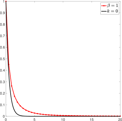
(a)

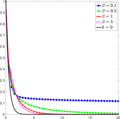
(b)

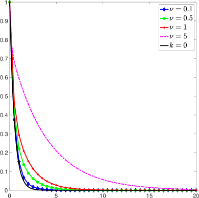
(c)

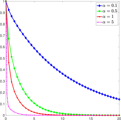
(d)

Figure 1. Plots of $s_{2\alpha}$ for $k(t)=\nu e^{-t^{\beta}}$.

2.1.2. Power-law kernels

We also implement the numerical scheme (2.1) in the case $k=\nu(1+t)^{-\beta-1}$. As Figure 2 shows, the decay is faster with the increase of $\beta$ (Figures LABEL:sub@fig:beta2), while it is slower with the rise of $\nu$ (Figure LABEL:sub@fig:nu2).

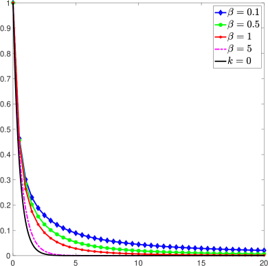
(a)

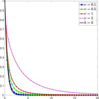
(b)

Figure 2. Plots of $s_{2\alpha}$ for $k=\nu(1+t)^{-\beta-1}$.

3. Proof of Theorems 1.1 and 1.2

To begin with, we introduce some notations and discuss some preliminary results.

3.1. The Ornstein-Uhlenbeck operator

We denote by

$$\gamma_{\alpha}(x)=\left(\frac{\alpha}{2\pi}\right)^{\frac{d}{2}}e^{-\frac{\alpha|x|^{2}}{2}}$$

a Gaussian distribution on ${\mathbb{R}}^{d}$ and by $d\gamma_{\alpha}(x)=\gamma_{\alpha}(x)dx$ the associated probability measure. For $\alpha=1$ we use the notation $\gamma=\gamma_{\alpha}$. $L^{2}(\gamma_{\alpha})$ is the space of measurable functions $f:{\mathbb{R}}^{d}\to{\mathbb{R}}$ such that $\int_{{\mathbb{R}}^{d}}|f|^{2}d\gamma_{\alpha}<\infty$, endowed with the usual scalar product $(\cdot,\cdot)_{L^{2}(\gamma_{\alpha})}$ and norm $\|\cdot\|_{L^{2}(\gamma_{\alpha})}.$ $H^{1}(\gamma_{\alpha})$ denotes the space of functions $f\in L^{2}(\gamma_{\alpha})$ such that $\nabla f\in L^{2}(\gamma_{\alpha})$, endowed with the norm

$$\|f\|_{H^{1}(\gamma_{\alpha})}:=\|f\|_{L^{2}(\gamma_{\alpha})}+\|\nabla f\|_{L^{2}(\gamma_{\alpha})}.$$

There are several ways to introduce the Ornstein-Uhlenbeck operator on $L^{2}(\gamma_{\alpha})$. Following [10], we consider the bilinear symmetric form $\mathcal{L}_{\alpha}:H^{1}(\gamma_{\alpha})\times H^{1}(\gamma_{\alpha})\to{\mathbb{R}}$ defined by

$$\mathcal{L}_{\alpha}(f,g):=\int_{{\mathbb{R}}^{d}}\nabla f\cdot\nabla g\ d\gamma_{\alpha},\qquad f,g\in H^{1}(\gamma_{\alpha}).$$

$\mathcal{L}_{\alpha}$ induces the operator $L_{\alpha}$ on $L^{2}(\gamma_{\alpha})$ defined by

(3.1) $$D(L_{\alpha}) =\{f\in H^{1}(\gamma_{\alpha})\,:\,\Delta f-\alpha x\cdot\nabla f\in L^{2}(\gamma_{\alpha})\},$$

$$L_{\alpha}f =\Delta f-\alpha x\cdot\nabla f,\qquad f\in D(L_{\alpha}),$$

that satisfies

$$\mathcal{L}_{\alpha}(f,g)=-(L_{\alpha}f,g)_{L^{2}(\gamma_{\alpha})},\qquad\forall g\in H^{1}(\gamma_{\alpha}),f\in D(L_{\alpha}).$$

$L_{\alpha}$ is the so-called Ornstein-Uhlenbeck operator. We recall that $L_{\alpha}$ is a negative self-adjoint operator, that generates a positive analytic semigroup $(T(t))_{t\geq 0}$ on $L^{2}(\gamma_{\alpha})$, see e.g. [1, Section 2.7.1].

For completeness we state and prove an integration by parts formula that will be useful in the sequel.

Lemma 3.1.

Let $L_{\alpha}$ be the Ornstein-Uhlenbeck operator. The following properties hold.

• For any $f\in D(L_{\alpha})$ there exists a sequence $\{f_{k}\}$ of functions belonging to $C_{c}^{\infty}({\mathbb{R}}^{d})$ such that $\nabla f_{k}\xrightarrow[\scriptscriptstyle k\to\infty]{}\nabla f$ and $L_{\alpha}(f_{k})\xrightarrow[\scriptscriptstyle k\to\infty]{}L_{\alpha}f$ in $L^{2}(\gamma_{\alpha})$.

• Assume $f\in D(L_{\alpha})$, $\mathcal{U}\subset{\mathbb{R}}$ an open set and $\Phi:\mathcal{U}\to{\mathbb{R}}$ a $C^{1}$-function. For any $g\in H^{1}(\gamma_{\alpha})$ such that $g(x)\in\mathcal{U}$ $\gamma_{\alpha}$-a.e. on ${\mathbb{R}}^{d}$, $\Phi(g)\in L^{2}(\gamma_{\alpha})$ and $\Phi^{\prime}(g)\in L^{\infty}(\gamma_{\alpha})$ we have

  (3.2) $$\int_{{\mathbb{R}}^{d}}L_{\alpha}f\ \Phi(g)d\gamma_{\alpha}=-\int_{{\mathbb{R}}^{d}}\Phi^{\prime}(g)\nabla f\cdot\nabla g\ d\gamma_{\alpha}.$$

Proof.

(i) The statement follows by means of the usual techniques of convolution and cut-off.

(ii) By (i) and the fact that $\Phi(g)\in L^{2}(\gamma_{\alpha})$ and $\Phi^{\prime}(g)\in L^{\infty}(\gamma_{\alpha})$, it is enough to prove (3.2) when $f$ belongs to $C^{\infty}_{c}({\mathbb{R}}^{d})$. Indeed, choose $R>0$ such that $\text{supp}(f)\subset B_{R}:=\{x\in{\mathbb{R}}^{d};|x|\leq R\}$, then

$$\int_{{\mathbb{R}}^{d}}L_{\alpha}f\ \Phi(g)d\gamma_{\alpha} =\int_{B_{R}}\Delta f\ \Phi(g)d\gamma_{\alpha}-\alpha\int_{B_{R}}x\cdot\nabla f\ \Phi(g)d\gamma_{\alpha}$$

$$=-\int_{B_{R}}\Phi^{\prime}(g)\nabla f\cdot\nabla g\ d\gamma_{\alpha},$$

that is (3.2). ∎

3.2. Evolutionary integral equations

The purpose of this section is to recall some well-known notions and results about integral equations.

We denote by $L_{loc}^{1}(0,\infty)$ (resp. $W_{\rm loc}^{1,1}(0,\infty)$, $W_{\rm loc}^{2,1}(0,\infty)$) the space of functions belonging to $L^{1}(0,T)$ (resp. $W^{1,1}(0,T)$, $W^{2,1}(0,T)$) for any $T\in(0,\infty)$.

For any $k,f\in L_{\rm loc}^{1}(0,\infty)$ the symbol $k*f$ stands for convolution from $0$ to $t$, that is

$$k*f\,(t)=\int_{0}^{t}k(t-s)f(s)\,ds,\qquad t\geq 0.$$

As usual, the Laplace transform of a function $f\in L^{1}_{loc}(0,\infty)$ having sub-exponential growth (i.e. for all $\omega>0$, $\int_{0}^{\infty}e^{-\omega t}|f(t)|dt<\infty$) will be denoted by

$$\widehat{f}(\lambda):=\int_{0}^{\infty}e^{-\lambda t}f(t)dt\qquad\lambda\in{\mathbb{C}},\ \Re\lambda>0.$$

Classical results for integral equations (see, e.g., [9, Theorem 2.3.5]) ensure that, for any kernel $k\in L_{loc}^{1}(0,\infty)$ and any $g\in L_{loc}^{1}(0,\infty)$, the problem

(3.3) $$f(t)+k*f(t)=g(t),\qquad t\geq 0\,,$$

admits a unique solution $f\in L_{loc}^{1}(0,\infty)$. Moreover, if $g\in W_{loc}^{1,1}(0,\infty)$ (resp. $W_{\rm loc}^{2,1}(0,\infty)$), then we have $f\in W_{loc}^{1,1}(0,\infty)$ (resp. $W_{\rm loc}^{2,1}(0,\infty)$) too.

It is useful to recall the following result, see [16, Lemma 1.3].

Lemma 3.2.

If $k\in L^{1}_{loc}(0,\infty)$ is non-negative and non-increasing and $g\in L^{1}_{loc}(0,\infty)$ is non-negative and non-decreasing, then the solution $\varphi$ of the integral equation (3.3) satisfies

(3.4) $$0\leq\varphi(t)\leq g(t)\qquad\mbox{for a.e.}\ t\geq 0\,.$$

Given $b\in L^{1}_{loc}(0,\infty)$, recall that $b$ is a kernel of positive type if

(3.5) $$\int_{0}^{T}b*v(t)v(t)\ dt\geq 0\,,\qquad\mbox{for any}\ T>0\,,\,v\in L^{2}(0,T).$$

If $b\in L^{\infty}(0,\infty)$, $b$ is of positive type if and only if

(3.6) $$\Re\;\widehat{b}(\lambda)\geq 0\,\qquad\mbox{for any}\,\lambda\in{\mathbb{C}}\,,\,\,\Re\lambda>0$$

(see, e.g., [21, p.38]).

Also, $b$ is said to be a completely positive kernel if there exists $k\in W^{1,1}_{loc}(0,\infty)$ non-negative and non-increasing such that

(3.7) $$b(t)+\int_{0}^{t}k(t-s)b(s)ds=1,\qquad t\geq 0.$$

Lemma 3.3.

If $b$ is a completely positive kernel, then we have

• $b\in W^{2,1}_{loc}(0,\infty)$;  $0\leq b(t)\leq 1$     $\forall t\geq 0$.

• If $k$ is the function in (3.7), then we have

  (3.8) $$\widehat{b}(\lambda)=\frac{1}{\lambda(1+\widehat{k}(\lambda))},\qquad\Re\lambda>0.$$

• $b$ is a kernel of positive type.

• For any $u_{0}\in{\mathbb{R}}$ and $f\in C([0,\infty))$, $u\in C([0,\infty))$ is given by

  (3.9) $$u(t)=u_{0}+b*f(t),\quad t\geq 0,$$

  if and only if $u\in C^{1}([0,\infty))$ and satisfies

  (3.10) $$\begin{cases}\dot{u}+k*\dot{u}(t)=f(t),\;\;\ t\geq 0,\cr u(0)=u_{0}\,.\end{cases}$$

Proof.

(i) Let $k\in W^{1,1}_{loc}(0,\infty)$ the non-negative and non-increasing function such that (3.7) holds. We can apply Lemma 3.2 with $g(t)\equiv 1$ to obtain $0\leq b(t)\leq 1$ for any $t\geq 0$.

(ii) Thanks to (i) and $0\leq k(t)\leq k(0)$, $t\geq 0$, we have $b,k\in L^{\infty}(0,\infty)$. Therefore, taking the Laplace transform of equation (3.7) we get

$$\widehat{b}(\lambda)\big{(}1+\widehat{k}(\lambda)\big{)}=\frac{1}{\lambda},\qquad\forall\Re\lambda>0,$$

and hence $1+\widehat{k}(\lambda)\not=0$, $\Re\lambda>0$, and (3.8) holds.

(iii) Since $b\in L^{\infty}(0,\infty)$ we will prove (3.6). Indeed, from (3.8) we deduce for $\Re\lambda>0$

$$\Re\widehat{b}(\lambda)=\frac{\Re\lambda+\Re\lambda\Re\widehat{k}(\lambda)-\Im\lambda\Im\widehat{k}(\lambda)}{\big{|}\lambda(1+\widehat{k}(\lambda))\big{|}^{2}}\,.$$

Integrating by parts, we have

$$\Re\lambda\Re\widehat{k}(\lambda)=\Re\lambda\int_{0}^{\infty}e^{-\Re\lambda t}\cos(\Im\lambda t)k(t)\ dt=-\int_{0}^{\infty}\partial_{t}(e^{-\Re\lambda t})\cos(\Im\lambda t)k(t)\ dt\\ =k(0)+\Im\lambda\Im\widehat{k}(\lambda)+\int_{0}^{\infty}e^{-\Re\lambda t}\cos(\Im\lambda t)\dot{k}(t)\ dt\,.$$

Thanks to $\dot{k}(t)\leq 0$ we note that

$$k(0)+\int_{0}^{\infty}e^{-\Re\lambda t}\cos(\Im\lambda t)\dot{k}(t)\ dt=\int_{0}^{\infty}\big{(}e^{-\Re\lambda t}\cos(\Im\lambda t)-1\big{)}\dot{k}(t)\ dt\geq 0,$$

and hence

$$\Re\lambda\Re\widehat{k}(\lambda)-\Im\lambda\Im\widehat{k}(\lambda)\geq 0,$$

that is $\Re\widehat{b}(\lambda)>0$ for $\Re\lambda>0$.

(iv) If $u$ is given by (3.9), then by $k*u$, using (3.7) and differentiating, we obtain (3.10). Vice versa, if we convolve the equation in (3.10) with $b$ and apply (3.7) we get

$$1*\dot{u}(t)=b*f(t),$$

hence we have (3.9). ∎

Let us introduce the functions $s_{\mu}(t)$ associated to a completely positive kernel $b$. By [21, Proposition 4.5], for any $\mu>0$ there exists a unique positive and non-increasing function $s_{\mu}\in C^{1}([0,\infty))$ such that

(3.11) $$s_{\mu}(t)+\mu b*s_{\mu}(t)=1,\qquad t\geq 0.$$

Thanks to Lemma 3.3-(iv), equation (3.11) can be written as

(3.12) $$\dot{s}_{\mu}(t)+k*\dot{s}_{\mu}(t)+\mu s_{\mu}(t)=0,\quad\ t\geq 0,\quad s_{\mu}(0)=1\,.$$

To estimate the entropy of the solutions to (1.1), for the non-local operator $k*\dot{u}$ we need an identity, which looks like an analogue of the chain rule, see [25].

Lemma 3.4.

Assume $k\in W_{loc}^{1,1}(0,\infty)$. Given $U$ an open subset of ${\mathbb{R}}$, $\Phi\in C^{1}(U)$ and $u\in W_{loc}^{1,1}(0,\infty)$, $u(t)\in U$ on $(0,\infty)$, then for $t\geq 0$

• $\displaystyle\begin{aligned} &\Phi^{\prime}(u(t))(k*\dot{u})(t)\\ =&k*\Big{(}\frac{d}{dt}\Phi(u)\Big{)}(t)+\big{(}\Phi(u(0))-\Phi(u(t))+\Phi^{\prime}(u(t))(u(t)-u(0))\big{)}k(t)\\ &-\int_{0}^{t}\Big{(}\Phi(u(t-s))-\Phi(u(t))-\Phi^{\prime}(u(t))\big{(}u(t-s)-u(t)\big{)}\Big{)}\dot{k}(s)ds.\end{aligned}$

• For a non-negative and non-increasing kernel $k$, assuming also that $\Phi$ is convex on $U$, we have

  (3.13) $$k*\Big{(}\frac{d}{dt}\Phi(u)\Big{)}(t)\leq\Phi^{\prime}(u(t))(k*\dot{u})(t),\quad t\geq 0.$$

Proof.

(i) Due to the assumptions, we have for $t\geq 0$

$$\frac{d}{dt}(k*u)(t) =k*\dot{u}(t)+k(t)u(0),$$

$$\frac{d}{dt}\big{(}k*\Phi(u)\big{)}(t) =k*\Big{(}\frac{d}{dt}\Phi(u)\Big{)}(t)+k(t)\Phi(u(0)).$$

The assertion follows by [25, Lemma 2.2] in virtue of the above identities.

(ii) As in [12, Corollary 6.1], by the convexity of $\Phi$, taking into account that $k\geq 0$ and $\dot{k}\leq 0$, the last two terms on the right-hand side of the identity in (i) are non-negative, so (3.13) follows. ∎

We also need a comparison result.

Lemma 3.5.

Assume that $k\in W^{1,1}_{loc}(0,\infty)$ is non-negative and non-increasing. Suppose that $u,v\in W^{1,1}_{loc}(0,\infty)$ satisfy $v(0)\leq w(0)$ and there exists a constant $C>0$ such that

(3.14) $$\dot{v}+k*\dot{v}+Cv\leq 0,\quad\dot{w}+k*\dot{w}+Cw\geq 0,\ \ \text{on}\ (0,\infty).$$

Then $v\leq w$ on $(0,\infty)$.

Proof.

The idea is essentially given in [25, Lemma 2.6]. Set $z=v-w$, we can apply (3.13) to the convex function $\Phi(y)=\frac{1}{2}y_{+}^{2}$, where $y_{+}:=\max\{y,0\}$, to get

$$\frac{d}{dt}z_{+}^{2}+k*\left(\frac{d}{dt}z_{+}^{2}\right)(t)\leq 2z_{+}\left(\dot{z}+k*\dot{z}\right).$$

By (3.14) it follows

$$\dot{z}+k*\dot{z}+Cz\leq 0,$$

and hence

$$\frac{d}{dt}z_{+}^{2}+k*\left(\frac{d}{dt}z_{+}^{2}\right)(t)+2C\,z\,z_{+}\leq 0.$$

Convolving with $b$ and applying (3.20) we have

$$z_{+}^{2}+2Cb*(z\,z_{+})\leq 0.$$

Since by Lemma 3.3-(i) $b$ is positive, thanks also to $z_{+}z=z_{+}^{2}$, it follows

$$z_{+}^{2}\leq z_{+}^{2}+2Cb*(z_{+}^{2})\leq 0,\quad\text{on}\ (0,\infty),$$

whence $v\leq w$ on $(0,\infty)$. ∎

3.3. Entropy and Logarithmic Sobolev Inequality

For $\alpha>0$ we denote by $d\gamma_{\alpha}$ the Gaussian measure on ${\mathbb{R}}^{d}$ defined as

$$d\gamma_{\alpha}(x):=\Big{(}\frac{\alpha}{2\pi}\Big{)}^{\frac{d}{2}}e^{-\frac{\alpha|x|^{2}}{2}}dx,$$

and set $d\gamma(x)=d\gamma_{1}(x)$. As well known, for a non-negative measurable function $f:{\mathbb{R}}^{d}\to{\mathbb{R}}$ such that $\int_{{\mathbb{R}}^{d}}f|\ln f|d\gamma_{\alpha}<\infty$ ($0\ln 0:=0$) the entropy of $f$ is given by

(3.15) $$\mathsf{Ent}f:=\int_{{\mathbb{R}}^{d}}f\ln fd\gamma_{\alpha}-\Big{(}\int_{{\mathbb{R}}^{d}}fd\gamma_{\alpha}\Big{)}\ln\Big{(}\int_{{\mathbb{R}}^{d}}fd\gamma_{\alpha}\Big{)}.$$

Note that, by Jensen inequality applied to $x\ln x$, it follows that $\mathsf{Ent}f\geq 0$. Moreover,

$$\mathsf{Ent}(cf)=c\,\mathsf{Ent}(f),\quad c>0.$$

Let us recall the following Logarithmic Sobolev Inequality.

Proposition 3.6.

Let $f\in H^{1}(\gamma_{\alpha})$ be. Then

(3.16) $$\mathsf{Ent}(f^{2})\leq\frac{2}{\alpha}\int_{{\mathbb{R}}^{d}}|\nabla f|^{2}d\gamma_{\alpha}.$$

In particular $f^{2}\ln(f^{2})\in L^{1}(\gamma_{\alpha})$. Moreover, the constant in (3.16) is optimal.

Proof.

If $\alpha=1$ inequality (3.16) becomes

(3.17) $$\mathsf{Ent}(f^{2})\leq 2\int_{{\mathbb{R}}^{d}}|\nabla f|^{2}d\gamma.$$

and the proof can be found in [10], see also [1, Proposition 5.5.1]. In the general case $\alpha>0$, set $f_{\alpha}(x)=f(\frac{x}{\sqrt{\alpha}})$ we observe that if $f\in H^{1}(\gamma_{\alpha})$, then $f_{\alpha}\in H^{1}(\gamma)$. Therefore, thanks also to (3.17), we have

$$\mathsf{Ent}(f^{2}) =\int_{{\mathbb{R}}^{d}}f^{2}\ln(f^{2})d\gamma_{\alpha}-\Big{(}\int_{{\mathbb{R}}^{d}}f^{2}d\gamma_{\alpha}\Big{)}\ln\Big{(}\int_{{\mathbb{R}}^{d}}f^{2}d\gamma_{\alpha}\Big{)}$$

$$=\int_{{\mathbb{R}}^{d}}f_{\alpha}^{2}\ln(f_{\alpha}^{2})d\gamma-\Big{(}\int_{{\mathbb{R}}^{d}}f_{\alpha}^{2}d\gamma\Big{)}\ln\Big{(}\int_{{\mathbb{R}}^{d}}f_{\alpha}^{2}d\gamma\Big{)}$$

$$\leq 2\int_{{\mathbb{R}}^{d}}|\nabla f_{\alpha}|^{2}d\gamma=\frac{2}{\alpha}\int_{{\mathbb{R}}^{d}}\Big{|}\nabla f\left(\frac{x}{\sqrt{\alpha}}\right)\Big{|}^{2}d\gamma=\frac{2}{\alpha}\int_{{\mathbb{R}}^{d}}|\nabla f|^{2}d\gamma_{\alpha}.$$

The optimality of the constant in the general case $\alpha>0$ follows by the optimality in the case $\alpha=1$. ∎

The following result gives the formulation of the Logarithmic Sobolev Inequality in terms of the Fisher information $\displaystyle\int_{{\mathbb{R}}^{d}}\frac{|\nabla g|^{2}}{g}d\gamma_{\alpha}$, where $g\in H^{1}(\gamma_{\alpha})$, $g\geq 0$ d$\gamma_{\alpha}$- a.e., see [1, p. 237].

Lemma 3.7.

Let $C>0$. The following assertions are equivalent.

• The Logarithmic Sobolev Inequality holds

  $$\mathsf{Ent}(f^{2})\leq C\int_{{\mathbb{R}}^{d}}|\nabla f|^{2}d\gamma_{\alpha},\qquad\text{for any}\ f\in H^{1}(\gamma_{\alpha}).$$

• The Entropy-Fisher Information Inequality holds

  $$\mathsf{Ent}(g)\leq\frac{C}{4}\int_{{\mathbb{R}}^{d}}\frac{|\nabla g|^{2}}{g}d\gamma_{\alpha},\qquad\text{for any}\ g\in H^{1}(\gamma_{\alpha}),\ g\geq 0\ d\gamma_{\alpha}-a.e..$$

3.4. Proof of Theorem 1.1.

Here we establish the well-posedness of the integro-differential problem

(3.18) $$\begin{cases}\dot{u}(t)+k*\dot{u}(t)=L_{\alpha}u(t),\;\;t>0\cr u(0)=u_{0}\,.\end{cases}$$

where the kernel $k$ satisfies the conditions

(3.19) $$k\in W^{1,1}_{loc}(0,\infty)\cap L^{1}(0,\infty),\quad k\ \mbox{is non-negative and non-increasing},$$

and $L_{\alpha}$ is the Ornstein-Uhlenbeck operator defined by (3.1).

Proof of Theorem 1.1.

Due to the assumption (3.19) on the kernel $k$, the unique solution $b\in W^{2,1}_{loc}(0,\infty)$ of the integral equation

(3.20) $$b(t)+\int_{0}^{t}k(t-s)b(s)ds=1,\qquad t>0,$$

is a completely positive kernel, see Section 3.2. By Lemma 3.3-(iv) for any $u_{0}\in D(L_{\alpha})$ we have that $u\in C^{1}([0,\infty);L^{2}(\gamma_{\alpha}))\cap C([0,\infty);D(L_{\alpha}))$ is a solution of (3.18) if and only if $u\in C([0,\infty);D(L_{\alpha}))$ is the solution of the integral equation

(3.21) $$u(t)=u_{0}+\int_{0}^{t}b(t-s)L_{\alpha}u(s)ds,\qquad t\geq 0.$$

Therefore, to solve (3.18) it is sufficient to prove the well-posedness for (3.21). To this end, we show that there exists the resolvent for (3.21), that is a family $\{S(t)\}_{t\geq 0}$ of linear bounded operators in $L^{2}(\gamma_{\alpha})$ such that

1. $S(0)=I$ and for $u_{0}\in L^{2}(\gamma_{\alpha})$ the map $t\mapsto S(t)u_{0}$ is continuous;

2. for $u_{0}\in D(L_{\alpha})$ and $t\geq 0$, one has $S(t)u_{0}\in D(L_{\alpha})$, $L_{\alpha}S(t)u_{0}=S(t)L_{\alpha}u_{0}$ and

   (3.22) $$S(t)u_{0}=u_{0}+\int_{0}^{t}b(t-s)L_{\alpha}S(s)u_{0}ds,\qquad t\geq 0.$$

First, we note that by Lemma 3.3-(iii) $b$ is a kernel of positive type. Since $L_{\alpha}$ generates an analytic semigroup (see Subsection 3.1), we can apply [21, Corollary 3.1] to have that equation (3.21) is parabolic. Moreover, in order to apply [21, Theorem 3.1], we have to show that $b$ is 1-regular, i.e. there exists $C>0$ such that $|\lambda\widehat{b}^{\prime}(\lambda)|\leq C|\widehat{b}(\lambda)|$ for all $\Re\lambda>0$. Indeed, thanks to (3.8) we have

$$\frac{\lambda\widehat{b}^{\prime}(\lambda)}{\widehat{b}(\lambda)}=-\frac{1+(\lambda\widehat{k}(\lambda))^{\prime}}{1+\widehat{k}(\lambda)}.$$

Now, also by an integration by parts we get

$$(\lambda\widehat{k}(\lambda))^{\prime}=\widehat{k}(\lambda)-\lambda\int_{0}^{\infty}e^{-\lambda t}tk(t)dt=-\widehat{t\dot{k}}(\lambda)\,,$$

and hence

$$\frac{\lambda\widehat{b}^{\prime}(\lambda)}{\widehat{b}(\lambda)}=\frac{\widehat{t\dot{k}}(\lambda)-1}{1+\widehat{k}(\lambda)}.$$

To prove the boundedness of the right hand-side, thanks to $k\in L^{1}(0,\infty)$, by Riemann-Lebesgue lemma we have $\widehat{k}(\lambda)\to 0$ as $|\lambda|\to\infty$. This implies that $1+\widehat{k}(\lambda)$ is bounded from below on $\{\Re\lambda>0\}$. In addition, integrating by parts we get

$$|\widehat{t\dot{k}}(\lambda)|\leq-\int_{0}^{\infty}e^{-\Re\lambda t}t\dot{k}(t)\ dt\\ =-\Re\lambda\int_{0}^{\infty}e^{-\Re\lambda t}tk(t)\ dt+\int_{0}^{\infty}e^{-\Re\lambda t}k(t)\ dt\leq\int_{0}^{\infty}k(t)\ dt\quad\forall\;\Re\lambda>0.$$

Therefore we have that $b$ is 1-regular. By Theorem [21, Theorem 3.1] we deduce the existence of the resolvent for the integral equation (3.21), that is a family $\{S(t)\}_{t\geq 0}$ of linear bounded operators in $L^{2}(\gamma_{\alpha})$ satisfying the conditions $(1)-(2)$. In particular, for any $u_{0}\in D(L_{\alpha})$ the function $S(t)u_{0}$ is the solution of (3.21), and hence $S(t)u_{0}$ is the strong solution of (3.18).

Moreover, if $u_{0}\in L^{2}(\gamma_{\alpha})$ $S(t)u_{0}$ is the weak solution of (3.18), since

$$S(t)u_{0}=\lim_{k\to\infty}S(t)u_{0k}\quad\text{in}\ L^{2}(\gamma_{\alpha}),$$

for any sequence $\{u_{0k}\}$ in $D(L_{\alpha})$ such that $u_{0k}\xrightarrow[k]{}u_{0}$ in $L^{2}(\gamma_{\alpha})$.

In addition, if we assume $u_{0}\geq 0$ $d\gamma_{\alpha}$– a.e., since $b$ is a completely positive kernel and $L_{\alpha}$ generates a positive semigroup on $L^{2}(\gamma_{\alpha})$, then by [20, Theorem 5] we have $S(t)u_{0}\geq 0$ $d\gamma_{\alpha}$– a.e., for any $t\geq 0$ . ∎

3.5. Proof of Theorem 1.2

In this subsection we show a sharp rate decay for the entropy of the solutions to problem (3.18) with the integral kernel $k$ satisfying (3.19).

To prove the statement we need the following two lemmas.

Lemma 3.8.

For any $u_{0}\in\ L^{2}(\gamma_{\alpha})$, $u_{0}\geq\varepsilon>0$ $d\gamma_{\alpha}$– a.e., the weak solution $u$ to problem (3.18) satisfies $u(t)\geq\varepsilon$ $d\gamma_{\alpha}$– a.e. for any $t\geq 0$.

Proof.

The assertion follows from Theorem 1.1, taking into account that the constant $\varepsilon$ is the unique solution to problem (3.18) when the initial condition is $\varepsilon$. ∎

Lemma 3.9 (Invariance).

Let $u_{0}\in L^{2}(\gamma_{\alpha})$. Then, the weak solution $u$ to problem (3.18) satisfies

(3.23) $$\int_{{\mathbb{R}}^{d}}u(t)\,d\gamma_{\alpha}=\int_{{\mathbb{R}}^{d}}u_{0}d\gamma_{\alpha},\quad\text{for any}\ t\geq 0.$$

Proof.

First, we consider $u_{0}\in D(L_{\alpha})$. By Theorem 1.1 $u$ is the strong solution to problem (3.18). Integrating the equation in (3.18) over ${\mathbb{R}}^{d}$, one has

$$\frac{d}{dt}\int_{{\mathbb{R}}^{d}}u(t)d\gamma_{\alpha}+k*\left(\frac{d}{dt}\int_{{\mathbb{R}}^{d}}u(t)d\gamma_{\alpha}\right)=\int_{{\mathbb{R}}^{d}}L_{\alpha}u(t)d\gamma_{\alpha}.$$

Applying Lemma 3.1-(ii) with $\Phi\equiv 1$ we get

$$\int_{{\mathbb{R}}^{d}}L_{\alpha}u(t)d\gamma_{\alpha}=0,$$

and hence

$$\frac{d}{dt}\int_{{\mathbb{R}}^{d}}u(t)d\gamma_{\alpha}+k*\left(\frac{d}{dt}\int_{{\mathbb{R}}^{d}}u(t)d\gamma_{\alpha}\right)=0.$$

Thanks to the uniqueness of the solutions of integral equations (3.3), we have

$$\frac{d}{dt}\int_{{\mathbb{R}}^{d}}u(t)d\gamma_{\alpha}\equiv 0,$$

that is (3.23).

The general assertion for $u_{0}\in L^{2}(\gamma_{\alpha})$ follows by means of approximation arguments. ∎

Proof of Theorem 1.2.

First, we prove the statement assuming the initial datum $u_{0}$ more regular, that is

(3.24) $$u_{0}\in D(L_{\alpha}),\qquad u_{0}\geq\varepsilon\ \ d\gamma_{\alpha}-\text{a.e.}.$$

By Theorem 1.1 problem (3.18) admits a unique strong solution $u$. Moreover, thanks to Lemma 3.8 one has $u(t)\geq\varepsilon$ $d\gamma_{\alpha}$– a.e. for any $t\geq 0$. Therefore, we can apply inequality (3.13) with $\Phi(\tau)=\tau\log(\tau)$, $\tau>0$, to get

$$\frac{d}{dt}\Phi(u(t))+k*\Big{(}\frac{d}{dt}\Phi(u)\Big{)}(t)\leq\Phi^{\prime}(u(t))\big{(}\dot{u}+k*\dot{u}\big{)}(t).$$

Integrating the above inequality, thanks also to the equation in (3.18), we obtain

$$\int_{{\mathbb{R}}^{d}}\frac{d}{dt}\Phi(u(t))+k*\Big{(}\frac{d}{dt}\Phi(u)\Big{)}(t)\ d\gamma_{\alpha}$$

$$\leq\int_{{\mathbb{R}}^{d}}\Phi^{\prime}(u(t))\big{(}\dot{u}+k*\dot{u}\big{)}(t)\ d\gamma_{\alpha}=\int_{{\mathbb{R}}^{d}}\Phi^{\prime}(u(t))L_{\alpha}u(t)\ d\gamma_{\alpha}.$$

Since $\Phi^{\prime}(u(t))=\ln u(t)+1\in L^{2}(\gamma_{\alpha})$ and $\Phi^{\prime\prime}(u(t))=\frac{1}{u(t)}\in L^{\infty}(\gamma_{\alpha})$, one can apply Lemma 3.1-(ii) to have

(3.25) $$\int_{{\mathbb{R}}^{d}}\Phi^{\prime}(u(t))L_{\alpha}u(t)\ d\gamma_{\alpha}=-\int_{{\mathbb{R}}^{d}}\frac{|\nabla u(t)|^{2}}{u(t)}d\gamma_{\alpha},$$

and hence

(3.26) $$\int_{{\mathbb{R}}^{d}}\frac{d}{dt}\Phi(u(t))+k*\Big{(}\frac{d}{dt}\Phi(u)\Big{)}(t)\ d\gamma_{\alpha}\leq-\int_{{\mathbb{R}}^{d}}\frac{|\nabla u(t)|^{2}}{u(t)}d\gamma_{\alpha}.$$

By (3.16) applied to the function $\sqrt{u(t)}$ we have

$$-\int_{{\mathbb{R}}^{d}}\frac{|\nabla u(t)|^{2}}{u(t)}d\gamma_{\alpha}\leq-2\alpha\mathsf{Ent}(u(t)).$$

Combining the above inequality with (3.26) one has

$$\int_{{\mathbb{R}}^{d}}\frac{d}{dt}\Phi(u(t))+k*\Big{(}\frac{d}{dt}\Phi(u)\Big{)}(t)\ d\gamma_{\alpha}\leq-2\alpha\mathsf{Ent}(u(t)).$$

Since

$$\mathsf{Ent}(u(t))=\int_{{\mathbb{R}}^{d}}\Phi(u(t))d\gamma_{\alpha}-\Phi\Big{(}\int_{{\mathbb{R}}^{d}}u(t)d\gamma_{\alpha}\Big{)}$$

and by Lemma 3.9 the function $\int_{{\mathbb{R}}^{d}}u(t)d\gamma_{\alpha}$ is constant, we have

(3.27) $$\frac{d}{dt}\mathsf{Ent}(u(t))=\int_{{\mathbb{R}}^{d}}\frac{d}{dt}\Phi(u(t)).$$

Therefore

$$\frac{d}{dt}\mathsf{Ent}(u(t))+k*\Big{(}\frac{d}{dt}\mathsf{Ent}(u)\Big{)}(t)+2\alpha\mathsf{Ent}(u(t))\leq 0.$$

Finally, taking into account (3.12) for $\mu=2\alpha$, that is

$$\dot{s}_{2\alpha}(t)+k*\dot{s}_{2\alpha}(t)+2\alpha s_{2\alpha}(t)=0,\quad\quad s_{2\alpha}(0)=1\,,$$

we can apply Lemma 3.5 to obtain inequality (1.11) for any $u_{0}$ satisfying (3.24).

In the general case we consider $u_{0}\in L^{2}(\gamma_{\alpha})$, $u_{0}\geq 0$ $d\gamma_{\alpha}$– a.e., and $u$ the weak solution to problem (3.18). By means of the usual techniques of convolution and cut-off we can construct a sequence $\{u_{0k}\}$ of functions belonging to $C^{\infty}_{c}({\mathbb{R}}^{d})$ such that

$$u_{0k}\geq 0\ d\gamma_{\alpha}-a.e.\quad\ \text{and}\quad u_{0k}\xrightarrow[k\to\infty]{}u_{0}\quad\text{ in }L^{2}(\gamma_{\alpha}).$$

Since $u_{0k}+\frac{1}{k}$ satisfy (3.24), denoted by $u_{k}$ the strong solution to problem (3.18) with initial datum $u_{0k}+\frac{1}{k}$, we have

(3.28) $$\mathsf{Ent}(u_{k}(t))\leq s_{2\alpha}(t)\mathsf{Ent}\Big{(}u_{0k}+\frac{1}{k}\Big{)},\qquad k\in{\mathbb{N}}.$$

Thanks to $u_{k}(t)\xrightarrow[k]{}u(t)$ in $L^{2}(\gamma_{\alpha})$, up to extract a subsequence, we can assume that $u_{k}(t)\xrightarrow[k]{}u(t)$ d$\gamma_{\alpha}$– a.e. and $|u_{k}(t)|\leq w(t)$, with $w(t)\in L^{2}(\gamma_{\alpha})$. Since for some $C>0$ one has $\tau|\ln\tau|\leq C(1+\tau^{2})$, $\tau>0$, we can apply Lebesgue dominated convergence theorem to get

$$\lim_{k\to\infty}\mathsf{Ent}(u_{k}(t))=\mathsf{Ent}(u(t)).$$

Similarly, applying again Lebesgue dominated convergence theorem, we also have

$$\lim_{k\to\infty}\mathsf{Ent}\Big{(}u_{0k}+\frac{1}{k}\Big{)}=\mathsf{Ent}(u_{0}),$$

and hence, letting $k\to\infty$ in (3.28), we obtain that inequality (1.11) holds.

To prove the optimality of the constant, we assume that, for $u_{0}$ satisfying (3.24) and some $\mu>0$, we have

(3.29) $$\mathsf{Ent}(u(t))\leq s_{\mu}(t)\mathsf{Ent}(u_{0}),\qquad t\geq 0.$$

Computing (3.27) at $t=0$, thanks also to (3.18) and (3.25) for $t=0$, one obtains,

(3.30) $$\frac{d}{dt}\mathsf{Ent}(u(t))\Big{|}_{t=0}=\int_{{\mathbb{R}}^{d}}\Phi^{\prime}(u_{0})L_{\alpha}u_{0}d\gamma_{\alpha}=-\int_{{\mathbb{R}}^{d}}\frac{|\nabla u_{0}|^{2}}{u_{0}}d\gamma_{\alpha}.$$

To estimate the left-hand side of (3.30), we note that by (3.29) it follows

$$\mathsf{Ent}(u(t))-\mathsf{Ent}(u_{0})\leq\big{(}s_{\mu}(t)-1\big{)}\mathsf{Ent}(u_{0}),$$

and hence, dividing for $t>0$ and sending $t\downarrow 0$, we obtain

(3.31) $$\frac{d}{dt}\mathsf{Ent}(u(t))\Big{|}_{t=0}\leq\dot{s}_{\mu}(0)\mathsf{Ent}(u_{0}).$$

Combining (3.30) with (3.31) and taking into account that $\dot{s}_{\mu}(0)=-\mu$, see (3.12), we get

(3.32) $$\mathsf{Ent}(u_{0})\leq\frac{1}{\mu}\int_{{\mathbb{R}}^{d}}\frac{|\nabla u_{0}|^{2}}{u_{0}}d\gamma_{\alpha},$$

that is, the Entropy-Fisher Information Inequality holds for $u_{0}$ satisfying (3.24). To apply Lemma 3.7 we have to prove (3.32) for any $u_{0}\in H^{1}(\gamma_{\alpha})$. To this end, first we fix $u_{0}\in D(L_{\alpha})$, $u_{0}\geq 0$ d$\gamma_{\alpha}$– a.e.. Since (3.32) holds for $u_{0}+\frac{1}{k}$, $k\in{\mathbb{N}}$, we have

$$\mathsf{Ent}\Big{(}u_{0}+\frac{1}{k}\Big{)}\leq\frac{1}{\mu}\int_{{\mathbb{R}}^{d}}\frac{|\nabla u_{0}|^{2}}{u_{0}+\frac{1}{k}}\ d\gamma_{\alpha}\leq\frac{1}{\mu}\int_{{\mathbb{R}}^{d}}\frac{|\nabla u_{0}|^{2}}{u_{0}}\ d\gamma_{\alpha}.$$

By Lebesgue dominated convergence theorem, letting $k\to\infty$ in the above inequality we obtain (3.32). Using again usual approximation arguments we deduce that (3.32) also holds for any $u_{0}\in H^{1}(\gamma_{\alpha})$, $u_{0}\geq 0$ d$\gamma_{\alpha}$– a.e.. Finally, we are able to apply Lemma 3.7: the Logarithmic Sobolev Inequality holds with constant $\frac{4}{\mu}$. Therefore, since the constant $\frac{2}{\alpha}$ in (3.16) is optimal, then we get $\frac{2}{\alpha}\leq\frac{4}{\mu}$, that is $\mu\leq 2\alpha$.

∎

4. Conclusions and extensions

In this article we study the effect of a time memory on the entropy decay of solutions to (1.1). Our main results concern the well-posedness and optimal entropy decay, see Theorems 1.1 and 1.2. Our assumption (1.2) on $k$ allows us to consider the stretched exponential functions (1.3), Caputo-Fabrizio operators and power-law kernels (1.5). Theorem 1.2 shows that the entropy decay of solutions to (1.1) is governed by the function $s_{2\alpha}$, which depends on the kernel $k$, because $s_{2\alpha}$ is the solution of the problem

(4.1) $$\dot{s}_{2\alpha}(t)+k*\dot{s}_{2\alpha}(t)+2\alpha s_{2\alpha}(t)=0,\quad\quad s_{2\alpha}(0)=1\,.$$

In Section 2, we explicitly compute the solution $s_{2\alpha}$ of (4.1) when $k(t)=\nu e^{-t}$, that is the case of Caputo-Fabrizio operators. For general stretched exponential and power-law kernels we implement numerical schemes to examine the behaviuor of $s_{2\alpha}$. As Figures 1 and 2 show, the effect of the memory in (1.1) weakens the decay of the entropy with respect to the case without memory $k\equiv 0$, in accordance with the physical behaviour of some materials, see [2].

The methods used in Section 3 seem flexible enough to study (1.1) in the case the Ornstein-Uhlenbeck operator is replaced by the operator $\Delta-\nabla W\cdot\nabla$ where $W$ is a potential. The latter type of operators and the relative Logarithmic Sobolev Inequality have been considered in [15] under suitable assumptions on the potential $W$. In this paper we consider the case $W(x)=\frac{\alpha}{2}|x|^{2}$.

Another possible extension is the study of the decay of a $\Phi$-entropy defined as

(4.2) $$\mathsf{Ent}_{\Phi}f:=\int_{{\mathbb{R}}^{d}}\Phi(f)d\gamma_{\alpha}-\Phi\Big{(}\int_{{\mathbb{R}}^{d}}fd\gamma_{\alpha}\Big{)},$$

where $\Phi:\mathcal{U}\to{\mathbb{R}}$ and $f$ takes its values in $\mathcal{U}$, for details we refer to [1, Section 7.6]. In the case $\Phi(\tau)=\tau\ln\tau$ and $\mathcal{U}=(0,\infty)$ the definition (4.2) coincide with (1.4).

References

- [1] D. Bakry, I. Gentil, and M. Ledoux. Analysis and geometry of Markov diffusion operators, volume 348 of Grundlehren der Mathematischen Wissenschaften. Springer, Cham, 2014.
- [2] M. Caputo and M. Fabrizio. A new definition of fractional derivative without singular kernel. Progr. Fract. Differ. Appl, 1:1–13, 2015.
- [3] M. Caputo and M. Fabrizio. On the notion of fractional derivative and applications to the hysteresis phenomena. Mecc., 52:3043–3052, 2017.
- [4] P. Clément and J. Prüss. Completely positive measures and Feller semigroups. Math. Ann., 287:73-–105, 1990.
- [5] M. A. F. dos Santos and I. S. Gomez. A fractional Fokker-Planck equation for non-singular kernel operators. J. Stat. Mech. Th. Exp. 12:1–13, 2018.
- [6] P. A. Feulefack, J. D. Djida, and A. Abdon. A new model of groundwater flow within an unconfined aquifer: application of Caputo-Fabrizio fractional derivative. Disc. Contin. Dyn. Syst. Ser. B, 24:3227–3247, 2019.
- [7] M. A. Firoozjaee, H. Jafari, A. Lia, and D. Baleanu. Numerical approach of Fokker-Planck equation with Caputo-Fabrizio fractional derivative using Ritz approximation. J. Comput. Appl. Math., 339:367–373, 2018.
- [8] J. F. Gómez-Aguilar, M. G. López-López, V. M. Alvarado-Martínez, J. Reyes-Reyes, and M. Adam-Medina. Modeling diffusive transport with a fractional derivative without singular kernel. Phys. A, 447:467–481, 2016.
- [9] G. Gripenberg, S.-O. Londen, and O. Staffans. Volterra integral and functional equations, volume 34 of Encyc. of Math. Appl.. Cambridge University Press, Cambridge, 1990.
- [10] L. Gross. Logarithmic Sobolev inequalities. Amer. J. Math., 97:1061–1083, 1975.
- [11] L. Hörmander. Hypoelliptic second order differential equations. Acta Math. 119:147-171, 1967.
- [12] J. Kemppainen, J. Siljander, V. Vergara, and R. Zacher. Decay estimates for time-fractional and other non-local in time subdiffusion equations in . Math. Ann., 366:941–979, 2016.
- [13] J. Kemppainen and R. Zacher. Long-time behavior of non-local in time Fokker-Planck equations via the entropy method. Math. Mod. Meth. Appl. Sci., 29:209–235, 2019.
- [14] M. A. Khan, Z. Hammouch, and D. Baleanu. Modeling the dynamics of hepatitis E via the Caputo-Fabrizio derivative. Math. Mod. Nat. Phenom., 14:Art. 311, p. 19, 2019.
- [15] M. Ledoux. Concentration of measure and logarithmic Sobolev inequalities. In Séminaire de Probabilités, XXXIII, Springer volume 1709 of Lect. Notes Math., p. 120–216, 1999.
- [16] J. J. Levin. Resolvents and bounds for linear and nonlinear Volterra equations. Trans. Amer. Math. Soc., 228:207–222, 1977.
- [17] J. C. Mauro, and Y. Z. Mauro. On the Prony series representation of stretched exponential relaxation. Phys. A, 506:75-87, 2018.
- [18] G. Metafune, D. Pallara, and E. Priola. Spectrum of Ornstein-Uhlenbeck operators in spaces with respect to invariant measures. J. Funct. Anal., 196:40–-60, 2002.
- [19] J. W. Nunziato. On heat conduction in materials with memory. Quart. Appl. Math., 29: 187–204, 1971.
- [20] J. Prüss. Positivity and regularity of hyperbolic Volterra equations in Banach spaces. Math. Ann., 279:317–344, 1987.
- [21] J. Prüss. Evolutionary integral equations and applications. Mod. Birk. Class. Reprint of the 1993 edition.
- [22] A. Quarteroni, R. Sacco, and F. Saleri. Num. math., volume 37. Springer Science & Business Media, 2010.
- [23] A. S. Shaikh and K. Sooppy Nisar. Transmission dynamics of fractional order typhoid fever model using Caputo-Fabrizio operator. Chaos Sol. Fract., 128:355–365, 2019.
- [24] V. E. Tarasov. Caputo-Fabrizio operator in terms of integer derivatives: memory or distributed lag? Comput. Appl. Math., 38: Art. 113, p. 15, 2019.
- [25] V. Vergara and R. Zacher. Optimal decay estimates for time-fractional and other nonlocal subdiffusion equations via energy methods. SIAM J. Math. Anal., 47:210–239, 2015.