Generalization in Reinforcement Learning with Selective Noise Injection and Information Bottleneck

Abstract

The ability for policies to generalize to new environments is key to the broad application of RL agents. A promising approach to prevent an agent’s policy from overfitting to a limited set of training environments is to apply regularization techniques originally developed for supervised learning. However, there are stark differences between supervised learning and RL. We discuss those differences and propose modifications to existing regularization techniques in order to better adapt them to RL. In particular, we focus on regularization techniques relying on the injection of noise into the learned function, a family that includes some of the most widely used approaches such as Dropout and Batch Normalization. To adapt them to RL, we propose Selective Noise Injection (SNI), which maintains the regularizing effect the injected noise has, while mitigating the adverse effects it has on the gradient quality. Furthermore, we demonstrate that the Information Bottleneck (IB) is a particularly well suited regularization technique for RL as it is effective in the low-data regime encountered early on in training RL agents. Combining the IB with SNI, we significantly outperform current state of the art results, including on the recently proposed generalization benchmark Coinrun.

1 Introduction

Deep Reinforcement Learning (rl) has been used to successfully train policies with impressive performance on a range of challenging tasks, including Atari [6, 16, 31], continuous control [35, 46] and tasks with long-ranged temporal dependencies [33]. In those settings, the challenge is to be able to successfully explore and learn policies complex enough to solve the training tasks. Consequently, the focus of these works was to improve the learning performance of agents in the training environment and less attention was being paid to generalization to testing environments.

However, being able to generalize is a key requirement for the broad application of autonomous agents. Spurred by several recent works showing that most rl agents overfit to the training environment [15, 58, 62, 65, 66], multiple benchmarks to evaluate the generalization capabilities of agents were proposed, typically by procedurally generating or modifying levels in video games [8, 11, 20, 21, 32, 63]. How to learn generalizable policies in these environments remains an open question, but early results have shown the use of regularization techniques (like weight decay, dropout and batch normalization) established in the supervised learning paradigm can also be useful for rl agents [11]. Our work builds on these results, but highlights two important differences between supervised learning and rl which need to be taken into account when regularizing agents.

First, because in rl the training data depends on the model and, consequently, the regularization method, stochastic regularization techniques like Dropout or BatchNorm can have adverse effects. For example, injecting stochasticity into the policy can lead to prematurely ending episodes, preventing the agent from observing future rewards. Furthermore, stochastic regularization can destabilize training through the learned critic and off-policy importance weights. To mitigate those adverse effects and effectively apply stochastic regularization techniques to rl, we propose Selective Noise Injection (sni). It selectively applies stochasticity only when it serves regularization and otherwise computes the output of the regularized networks deterministically. We focus our evaluation on Dropout and the Variational Information Bottleneck (vib), but the proposed method is applicable to most forms of stochastic regularization.

A second difference between rl and supervised learning is the non-stationarity of the data-distribution in rl. Despite many rl algorithms utilizing millions or even billions of observations, the diversity of states encountered early on in training can be small, making it difficult to learn general features. While it remains an open question as to why deep neural networks generalize despite being able to perfectly memorize the training data [5, 64], it has been shown that the optimal point on the worst-case generalization bound requires the model to rely on a more compressed set of features the fewer data-points we have [47, 54]. Therefore, to bias our agent towards more general features even early on in training, we adapt the Information Bottleneck (ib) principle to an actor-critic agent, which we call Information Bottleneck Actor Critic (ibac). In contrast to other regularization techniques, ibac directly incentivizes the compression of input features, resulting in features that are more robust under a shifting data-distribution and that enable better generalization to held-out test environments.

We evaluate our proposed techniques using Proximal Policy Optimization (ppo), an off-policy actor-critic algorithm, on two challenging generalization tasks, Multiroom [9] and Coinrun [11]. We show the benefits of both ibac and sni individually as well as in combination, with the resulting ibac-sni significantly outperforming the previous state of the art results.

2 Background

We consider having a distribution $q(m)$ of Markov decision processes (mdps) $m\in\mathcal{M}$, with $m$ being a tuple $(\mathcal{S}_{m},\mathcal{A},T_{m},R_{m},p_{m})$ consisting of state-space $\mathcal{S}_{m}$, action-space $\mathcal{A}$, transition distribution $T_{m}(s^{\prime}|s,a)$, reward function $R_{m}(s,a)$ and initial state distribution $p_{m}(s_{0})$ [38]. For training, we either assume unlimited access to $q(m)$ (like in section 5.2, Multiroom) or restrict ourselves to a fixed set of training environments $M_{\text{train}}=\{m_{1},\dots,m_{n}\}$, $m_{i}\sim q$ (like in section 5.3, Coinrun).

The goal of the learning process is to find a policy $\pi_{\theta}(a|s)$, parameterized by $\theta$, which maximizes the discounted expected reward: $J(\pi_{\theta})=\mathbb{E}_{q,\pi,T_{m},p_{m}}\left[\sum_{t=0}^{T}\gamma^{t}R_{m}(s_{t},a_{t})\right]$. Although any rl method with an off-policy correction term could be used with our proposed method of sni, ppo [46] has shown strong performance and enables direct comparison with prior work [11]. The actor-critic version of this algorithm collects trajectory data $\mathcal{D}_{\tau}$ using a rollout policy $\pi^{r}_{\theta}(a_{t}|s_{t})$ and subsequently optimizes a surrogate loss:

$$L_{\lx@glossaries@gls@link{acronym}{PPO}{\leavevmode\textsc{ppo}}}=-\mathbb{E}_{\mathcal{D}_{\tau}}\left[\min(c_{t}(\theta)A_{t},\text{clip}(c_{t}(\theta),1-\epsilon,1+\epsilon)A_{t})\right]$$ (1)

with $c_{t}(\theta)=\frac{\pi_{\theta}(a_{t}|s_{t})}{\pi_{\theta}^{r}(a_{t}|s_{t})}$ for $K$ epochs. The advantage $A_{t}$ is computed as in A2C [30]. This is an efficient approximate trust region method [44], optimizing a pessimistic lower bound of the objective function on the collected data. It corresponds to estimating the gradient w.r.t the policy conservatively, since moving $\pi_{\theta}$ further away from $\pi_{\theta}^{r}$, such that $c_{t}(\theta)$ moves outside a chosen range $[1-\epsilon,1+\epsilon]$, is only taken into account if it decreases performance. Similarly, the value function loss minimizes an upper bound on the squared error:

$$L_{\lx@glossaries@gls@link{acronym}{PPO}{\leavevmode\textsc{ppo}}}^{V}=\mathbb{E}_{\mathcal{D}_{\tau}}\left[\frac{1}{2}\max\left((V_{\theta}-V^{T})^{2},(V^{r}+\text{clip}(V_{\theta}-V^{r},1-\epsilon,1+\epsilon)-V_{\text{target}})^{2}\right)\right]$$ (2)

with a bootstrapped value function target $V_{\text{target}}$ [30] and previous value function $V^{r}$. The overall minimization objective is then:

$$L_{t}(\theta)=L_{\lx@glossaries@gls@link{acronym}{PPO}{\leavevmode\textsc{ppo}}}+\lambda_{V}L_{\lx@glossaries@gls@link{acronym}{PPO}{\leavevmode\textsc{ppo}}}^{V}-\lambda_{H}H[\pi_{\theta}]$$ (3)

where $H[\cdot]$ denotes an entropy bonus to encourage exploration and prevent the policy to collapse prematurely. In the following, we discuss regularization techniques that can be used to mitigate overfitting to the states and mdps so far seen during training.

2.1 Regularization Techniques in Supervised Learning

In supervised learning, classifiers are often regularized using a variety of techniques to prevent overfitting. Here, we briefly present several major approaches which we either utilize as baseline or extend to rl in section 4.

Weight decay, also called L2 regularization, reduces the magnitude of the weights $\theta$ by adding an additional loss term $\lambda_{w}\frac{1}{2}\|\theta\|^{2}_{2}$. With a gradient update of the form $\theta\leftarrow\theta-\alpha\nabla_{\theta}(L(\theta)+\frac{\lambda_{w}}{2}\|\theta\|^{2}_{2})$, this decays the weights in addition to optimizing $L(\theta)$, i.e. we have $\theta\leftarrow(1-\alpha\lambda_{w})\theta-\alpha\nabla_{\theta}L(\theta)$.

Data augmentation refers to changing or distorting the available input data to improve generalization. In this work, we use a modified version of cutout [12], proposed by [11], in which a random number of rectangular areas in the input image is filled by random colors.

Batch Normalization [17, 18] normalizes activations of specified layers by estimating their mean and variance using the current mini-batch. Estimating the batch statistics introduces noise which has been shown to help improve generalization [28] in supervised learning.

Another widely used regularization technique for deep neural networks is Dropout [48]. Here, during training, individual activations are randomly zeroed out with a fixed probability $p_{d}$. This serves to prevent co-adaptation of neurons and can be applied to any layer inside the network. One common choice, which we are following in our architecture, is to apply it to the last hidden layer.

Lastly, we will briefly describe the Variational Information Bottleneck (vib)[2], a deep variational approximation to the Information Bottleneck (ib)[53]. While not typically used for regularization in deep supervised learning, we demonstrate in section 5 that our adaptation ibac shows strong performance in rl. Given a data distribution $p(X,Y)$, the learned model $p_{\theta}(y|x)$ is regularized by inserting a stochastic latent variable $Z$ and minimizing the mutual information between the input $X$ and $Z$, $I(X,Z)$, while maximizing the predictive power of the latent variable, i.e. $I(Z,Y)$. The vib objective function is:

$$L_{\text{VIB}}=\mathbb{E}_{p(x,y),p_{\theta}(z|x)}\big{[}-\log q_{\theta}(y|z)+\beta D_{KL}[p_{\theta}(z|x)\|q(z)]\big{]}$$ (4)

where $p_{\theta}(z|x)$ is the encoder, $q_{\theta}(y|z)$ the decoder, $q(z)$ the approximated latent marginal often fixed to a normal distribution $\mathcal{N}(0,I)$ and $\beta$ is a hyperparameter. For a normal distributed $p_{\theta}(z|x)$, eq. 4 can be optimized by gradient decent using the reparameterization trick [25].

3 The Problem of Using Stochastic Regularization in RL

We now take a closer look at a prototypical objective for training actor-critic methods and highlight important differences to supervised learning. Based on those observations, we propose an explanation for the finding that some stochastic optimization methods are less effective [11] or can even be detrimental to performance when combined with other regularization techniques (see appendix D).

In supervised learning, the optimization objective takes a form similar to $\max_{\theta}\mathbb{E}_{\mathcal{D}}\left[\log{\color[rgb]{0,0,1}\definecolor[named]{pgfstrokecolor}{rgb}{0,0,1}p_{\theta}(y|x)}\right]$, where we highlight the model ${\color[rgb]{0,0,1}\definecolor[named]{pgfstrokecolor}{rgb}{0,0,1}p_{\theta}(y|x)}$ to be updated in blue, $\mathcal{D}$ is the available data and $\theta$ the parameters to be learned. On the other hand, in rl the objective for the actor is to maximize $J(\pi_{\theta})=\mathbb{E}_{\color[rgb]{0,0,1}\definecolor[named]{pgfstrokecolor}{rgb}{0,0,1}\pi_{\theta}(a|s)}\left[\sum_{t}\gamma^{t}R_{m}(s_{t},a_{t})\right]$, where, for convencience, we drop $q$, $T_{m}$ and $p_{m}$ from the notation of the expectation. Because now the learned distribution, ${\color[rgb]{0,0,1}\definecolor[named]{pgfstrokecolor}{rgb}{0,0,1}\pi_{\theta}(a|s)}$, is part of data-generation, computing the gradients, as done in policy gradient methods, requires the log-derivative trick. For the class of deep off-policy actor-critic methods we are experimentally evaluating in this paper, one also typically uses the policy gradient theorem [52] and an estimated critic $V_{\theta}(s)$ as baseline and for bootstrapping to reduce the gradient variance. Consequently, the gradient estimation becomes:

$$\nabla_{\theta}J({\pi_{\theta}})=\mathbb{E}_{\color[rgb]{1,0.23,0.13}\definecolor[named]{pgfstrokecolor}{rgb}{1,0.23,0.13}\pgfsys@color@cmyk@stroke{0}{0.77}{0.87}{0}\pgfsys@color@cmyk@fill{0}{0.77}{0.87}{0}\pi^{r}_{\theta}(a_{t}|s_{t})}\left[\sum_{t}^{T}\frac{\color[rgb]{0,0,1}\definecolor[named]{pgfstrokecolor}{rgb}{0,0,1}\pi_{\theta}(a_{t}|s_{t})}{{\color[rgb]{1,0.23,0.13}\definecolor[named]{pgfstrokecolor}{rgb}{1,0.23,0.13}\pgfsys@color@cmyk@stroke{0}{0.77}{0.87}{0}\pgfsys@color@cmyk@fill{0}{0.77}{0.87}{0}\pi^{r}_{\theta}(a_{t}|s_{t})}}\nabla_{\theta}{\color[rgb]{0,0,1}\definecolor[named]{pgfstrokecolor}{rgb}{0,0,1}\log\pi_{\theta}(a_{t}|s_{t})}(r_{t}+\gamma{\color[rgb]{1,0.23,0.13}\definecolor[named]{pgfstrokecolor}{rgb}{1,0.23,0.13}\pgfsys@color@cmyk@stroke{0}{0.77}{0.87}{0}\pgfsys@color@cmyk@fill{0}{0.77}{0.87}{0}V_{\theta}(s_{t+1})-V_{\theta}(s_{t})})\right]$$ (5)

where we utilize a rollout policy ${\color[rgb]{1,0.23,0.13}\definecolor[named]{pgfstrokecolor}{rgb}{1,0.23,0.13}\pgfsys@color@cmyk@stroke{0}{0.77}{0.87}{0}\pgfsys@color@cmyk@fill{0}{0.77}{0.87}{0}\pi^{r}_{\theta}}$ to collect trajectories. It can deviate from $\color[rgb]{0,0,1}\definecolor[named]{pgfstrokecolor}{rgb}{0,0,1}\pi_{\theta}$ but should be similar to keep the off-policy correction term ${\nicefrac{{\color[rgb]{0,0,1}\definecolor[named]{pgfstrokecolor}{rgb}{0,0,1}\pi_{\theta}}}{{\color[rgb]{1,0.23,0.13}\definecolor[named]{pgfstrokecolor}{rgb}{1,0.23,0.13}\pgfsys@color@cmyk@stroke{0}{0.77}{0.87}{0}\pgfsys@color@cmyk@fill{0}{0.77}{0.87}{0}\pi^{r}_{\theta}}}}$ low variance. In eq. 5, only the term ${\color[rgb]{0,0,1}\definecolor[named]{pgfstrokecolor}{rgb}{0,0,1}\pi_{\theta}(a_{t}|s_{t})}$ is being updated and we highlight in orange all the additional influences of the learned policy and critic on the gradient.

Denoting by the superscript $\perp$ that $\color[rgb]{1,0.23,0.13}\definecolor[named]{pgfstrokecolor}{rgb}{1,0.23,0.13}\pgfsys@color@cmyk@stroke{0}{0.77}{0.87}{0}\pgfsys@color@cmyk@fill{0}{0.77}{0.87}{0}V_{\theta}^{\perp}$ is assumed constant, we can write the optimization objective for the critic as

$$L_{\text{AC}}^{V}=\min_{\theta}\mathbb{E}_{\color[rgb]{1,0.23,0.13}\definecolor[named]{pgfstrokecolor}{rgb}{1,0.23,0.13}\pgfsys@color@cmyk@stroke{0}{0.77}{0.87}{0}\pgfsys@color@cmyk@fill{0}{0.77}{0.87}{0}\pi^{r}_{\theta}(a_{t}|s_{t})}\left[\left(\gamma{\color[rgb]{1,0.23,0.13}\definecolor[named]{pgfstrokecolor}{rgb}{1,0.23,0.13}\pgfsys@color@cmyk@stroke{0}{0.77}{0.87}{0}\pgfsys@color@cmyk@fill{0}{0.77}{0.87}{0}V_{\theta}^{\perp}(s_{t+1})}+r_{t}-{\color[rgb]{0,0,1}\definecolor[named]{pgfstrokecolor}{rgb}{0,0,1}V_{\theta}(s_{t})}\right)^{2}\right]$$ (6)

From eqs. 5 and 6 we can see that the injection of noise into the computation of ${\color[rgb]{1,0.23,0.13}\definecolor[named]{pgfstrokecolor}{rgb}{1,0.23,0.13}\pgfsys@color@cmyk@stroke{0}{0.77}{0.87}{0}\pgfsys@color@cmyk@fill{0}{0.77}{0.87}{0}\pi_{\theta}^{r}}$ and ${\color[rgb]{1,0.23,0.13}\definecolor[named]{pgfstrokecolor}{rgb}{1,0.23,0.13}\pgfsys@color@cmyk@stroke{0}{0.77}{0.87}{0}\pgfsys@color@cmyk@fill{0}{0.77}{0.87}{0}V_{\theta}}$ can degrade performance in several ways: i) During rollouts using the rollout policy ${\color[rgb]{1,0.23,0.13}\definecolor[named]{pgfstrokecolor}{rgb}{1,0.23,0.13}\pgfsys@color@cmyk@stroke{0}{0.77}{0.87}{0}\pgfsys@color@cmyk@fill{0}{0.77}{0.87}{0}\pi_{\theta}^{r}}$, it can lead to undesirable actions, potentially ending episodes prematurely, and thereby deteriorating the quality of the observed data; ii) It leads to a higher variance of the off-policy correction term $\nicefrac{{\color[rgb]{0,0,1}\definecolor[named]{pgfstrokecolor}{rgb}{0,0,1}\pi_{\theta}}}{{\color[rgb]{1,0.23,0.13}\definecolor[named]{pgfstrokecolor}{rgb}{1,0.23,0.13}\pgfsys@color@cmyk@stroke{0}{0.77}{0.87}{0}\pgfsys@color@cmyk@fill{0}{0.77}{0.87}{0}\pi^{r}_{\theta}}}$ because the injected noise can be different for $\color[rgb]{0,0,1}\definecolor[named]{pgfstrokecolor}{rgb}{0,0,1}\pi_{\theta}$ and $\color[rgb]{1,0.23,0.13}\definecolor[named]{pgfstrokecolor}{rgb}{1,0.23,0.13}\pgfsys@color@cmyk@stroke{0}{0.77}{0.87}{0}\pgfsys@color@cmyk@fill{0}{0.77}{0.87}{0}\pi_{\theta}^{r}$, increasing gradient variance; iii) It increases variance in the gradient updates of both the policy and the critic through variance in the computation of ${\color[rgb]{1,0.23,0.13}\definecolor[named]{pgfstrokecolor}{rgb}{1,0.23,0.13}\pgfsys@color@cmyk@stroke{0}{0.77}{0.87}{0}\pgfsys@color@cmyk@fill{0}{0.77}{0.87}{0}V_{\theta}}$.

4 Method

To utilize the strength of noise-injecting regularization techniques in rl, we introduce Selective Noise Injection (sni)in the following section. Its goal is to allow us to make use of such techniques while mitigating the adverse effects the added stochasticity can have on the rl gradient computation. Then, in section 4.2, we propose Information Bottleneck Actor Critic (ibac)as a new regularization method and detail how sni applies to ibac, resulting in our state-of-the art method ibac-sni.

4.1 Selective Noise Injection

We have identified three sources of negative effects due to noise which we need to mitigate: In the rollout policy ${\color[rgb]{1,0.23,0.13}\definecolor[named]{pgfstrokecolor}{rgb}{1,0.23,0.13}\pgfsys@color@cmyk@stroke{0}{0.77}{0.87}{0}\pgfsys@color@cmyk@fill{0}{0.77}{0.87}{0}\pi^{r}_{\theta}}$, in the critic ${\color[rgb]{1,0.23,0.13}\definecolor[named]{pgfstrokecolor}{rgb}{1,0.23,0.13}\pgfsys@color@cmyk@stroke{0}{0.77}{0.87}{0}\pgfsys@color@cmyk@fill{0}{0.77}{0.87}{0}V_{\theta}}$ and in the off-policy correction term $\nicefrac{{\color[rgb]{0,0,1}\definecolor[named]{pgfstrokecolor}{rgb}{0,0,1}\pi_{\theta}}}{{\color[rgb]{1,0.23,0.13}\definecolor[named]{pgfstrokecolor}{rgb}{1,0.23,0.13}\pgfsys@color@cmyk@stroke{0}{0.77}{0.87}{0}\pgfsys@color@cmyk@fill{0}{0.77}{0.87}{0}\pi^{r}_{\theta}}}$. We first introduce a short notation for eq. 5 as $\nabla_{\theta}J(\pi_{\theta})=\mathcal{G}_{\lx@glossaries@gls@link{acronym}{AC}{\leavevmode\textsc{ac}}}({\color[rgb]{1,0.23,0.13}\definecolor[named]{pgfstrokecolor}{rgb}{1,0.23,0.13}\pgfsys@color@cmyk@stroke{0}{0.77}{0.87}{0}\pgfsys@color@cmyk@fill{0}{0.77}{0.87}{0}\pi^{r}_{\theta}},{\color[rgb]{0,0,1}\definecolor[named]{pgfstrokecolor}{rgb}{0,0,1}\pi_{\theta}},{\color[rgb]{1,0.23,0.13}\definecolor[named]{pgfstrokecolor}{rgb}{1,0.23,0.13}\pgfsys@color@cmyk@stroke{0}{0.77}{0.87}{0}\pgfsys@color@cmyk@fill{0}{0.77}{0.87}{0}V_{\theta}})$.

To apply sni to a regularization technique relying on noise-injection, we need to be able to temporarily suspend the noise and compute the output of the model deterministically. This is possible for most techniques: For example, in Dropout, we can freeze one particular dropout mask, in vib we can pass in the mode instead of sampling from the posterior distribution and in Batch Normalization we can either utilize the moving average instead of the batch statistics or freeze and re-use one statistic multiple times. Formally, we denote by $\bar{\pi}_{\theta}$ the version of a component $\pi_{\theta}$, with the injected regularization noise suspended. Note that this does not mean that $\bar{\pi}_{\theta}$ is deterministic, for example when the network approximates the parameters of a distribution.

Then, for sni we modify the policy gradient loss as follows: i) We use $\color[rgb]{1,0.23,0.13}\definecolor[named]{pgfstrokecolor}{rgb}{1,0.23,0.13}\pgfsys@color@cmyk@stroke{0}{0.77}{0.87}{0}\pgfsys@color@cmyk@fill{0}{0.77}{0.87}{0}\bar{V}_{\theta}$ as critic instead of $\color[rgb]{1,0.23,0.13}\definecolor[named]{pgfstrokecolor}{rgb}{1,0.23,0.13}\pgfsys@color@cmyk@stroke{0}{0.77}{0.87}{0}\pgfsys@color@cmyk@fill{0}{0.77}{0.87}{0}V_{\theta}$ in both eqs. 5 and 6, eliminating unnecessary noise through the critic; ii) We use $\color[rgb]{1,0.23,0.13}\definecolor[named]{pgfstrokecolor}{rgb}{1,0.23,0.13}\pgfsys@color@cmyk@stroke{0}{0.77}{0.87}{0}\pgfsys@color@cmyk@fill{0}{0.77}{0.87}{0}\bar{\pi}^{r}$ as rollout policy instead of $\color[rgb]{1,0.23,0.13}\definecolor[named]{pgfstrokecolor}{rgb}{1,0.23,0.13}\pgfsys@color@cmyk@stroke{0}{0.77}{0.87}{0}\pgfsys@color@cmyk@fill{0}{0.77}{0.87}{0}\pi^{r}$. For some regularization techniques this will reduce the probability of undesirable actions; iii) We compute the policy gradient as a mixture between gradients for $\color[rgb]{0,0,1}\definecolor[named]{pgfstrokecolor}{rgb}{0,0,1}\pi_{\theta}$ and $\color[rgb]{0,0,1}\definecolor[named]{pgfstrokecolor}{rgb}{0,0,1}\bar{\pi}_{\theta}$ as follows:

$$\mathcal{G}^{\lx@glossaries@gls@link{acronym}{SNI}{\leavevmode\textsc{sni}}}_{\lx@glossaries@gls@link{acronym}{AC}{\leavevmode\textsc{ac}}}({\color[rgb]{1,0.23,0.13}\definecolor[named]{pgfstrokecolor}{rgb}{1,0.23,0.13}\pgfsys@color@cmyk@stroke{0}{0.77}{0.87}{0}\pgfsys@color@cmyk@fill{0}{0.77}{0.87}{0}\pi_{\theta}^{r}},{\color[rgb]{0,0,1}\definecolor[named]{pgfstrokecolor}{rgb}{0,0,1}\pi_{\theta}},{\color[rgb]{1,0.23,0.13}\definecolor[named]{pgfstrokecolor}{rgb}{1,0.23,0.13}\pgfsys@color@cmyk@stroke{0}{0.77}{0.87}{0}\pgfsys@color@cmyk@fill{0}{0.77}{0.87}{0}V_{\theta}})=\lambda\mathcal{G}_{\lx@glossaries@gls@link{acronym}{AC}{\leavevmode\textsc{ac}}}({\color[rgb]{1,0.23,0.13}\definecolor[named]{pgfstrokecolor}{rgb}{1,0.23,0.13}\pgfsys@color@cmyk@stroke{0}{0.77}{0.87}{0}\pgfsys@color@cmyk@fill{0}{0.77}{0.87}{0}\bar{\pi}_{\theta}^{r}},{\color[rgb]{0,0,1}\definecolor[named]{pgfstrokecolor}{rgb}{0,0,1}\bar{\pi}_{\theta}},{\color[rgb]{1,0.23,0.13}\definecolor[named]{pgfstrokecolor}{rgb}{1,0.23,0.13}\pgfsys@color@cmyk@stroke{0}{0.77}{0.87}{0}\pgfsys@color@cmyk@fill{0}{0.77}{0.87}{0}\bar{V}_{\theta}})+(1-\lambda)\mathcal{G}_{\lx@glossaries@gls@link{acronym}{AC}{\leavevmode\textsc{ac}}}({\color[rgb]{1,0.23,0.13}\definecolor[named]{pgfstrokecolor}{rgb}{1,0.23,0.13}\pgfsys@color@cmyk@stroke{0}{0.77}{0.87}{0}\pgfsys@color@cmyk@fill{0}{0.77}{0.87}{0}\bar{\pi}_{\theta}^{r}},{\color[rgb]{0,0,1}\definecolor[named]{pgfstrokecolor}{rgb}{0,0,1}\pi_{\theta}},{\color[rgb]{1,0.23,0.13}\definecolor[named]{pgfstrokecolor}{rgb}{1,0.23,0.13}\pgfsys@color@cmyk@stroke{0}{0.77}{0.87}{0}\pgfsys@color@cmyk@fill{0}{0.77}{0.87}{0}\bar{V}_{\theta}})$$ (7)

The first term guarantees a lower variance of the off-policy importance weight, which is especially important early on in training when the network has not yet learned to compensate for the injected noise. The second term uses the noise-injected policy for updates, thereby taking advantage of its regularizing effects while still reducing unnecessary variance through the use of $\color[rgb]{1,0.23,0.13}\definecolor[named]{pgfstrokecolor}{rgb}{1,0.23,0.13}\pgfsys@color@cmyk@stroke{0}{0.77}{0.87}{0}\pgfsys@color@cmyk@fill{0}{0.77}{0.87}{0}\bar{\pi}^{r}$ and $\color[rgb]{1,0.23,0.13}\definecolor[named]{pgfstrokecolor}{rgb}{1,0.23,0.13}\pgfsys@color@cmyk@stroke{0}{0.77}{0.87}{0}\pgfsys@color@cmyk@fill{0}{0.77}{0.87}{0}\bar{V}_{\theta}$. Note that sharing the rollout policy $\color[rgb]{1,0.23,0.13}\definecolor[named]{pgfstrokecolor}{rgb}{1,0.23,0.13}\pgfsys@color@cmyk@stroke{0}{0.77}{0.87}{0}\pgfsys@color@cmyk@fill{0}{0.77}{0.87}{0}\bar{\pi}^{r}$ between both terms allows us to use the same collected data. Furthermore most computations are shared between both terms or can be parallelized.

4.2 Information Bottleneck Actor Critic

Early on in training an rl agent, we are often faced with little variation in the training data. Observed states are distributed only around the initial states $s_{0}$, making spurious correlations in the low amount of data more likely. Furthermore, because neither the policy nor the critic have sufficiently converged yet, we have a high variance in the target values of our loss function.

This combination makes it harder and less likely for the network to learn desirable features that are robust under a shifting data-distribution during training and generalize well to held-out test mdps. To counteract this reduced signal-to-noise ratio, our goal is to explicitly bias the learning towards finding more compressed features which are shown to have a tighter worst-case generalization bound [54]. While a higher compression does not guarantee robustness under a shifting data-distribution, we believe this to be a reasonable assumption in the majority of mdps, for example because they rely on a consistent underlying transition mechanism like physical laws.

To incentivize more compressed features, we use an approach similar to the vib [2], which minimizes the mutual information $I(S,Z)$ between the state $S$ and its latent representation $Z$ while maximizing $I(Z,A)$, the predictive power of $Z$ on actions $A$. To do so, we re-interpret the policy gradient update as maximization of the log-marginal likelihood of $\pi_{\theta}(a|s)$ under the data distribution $p(s,a)\mathrel{\mathop{\mathchar 58\relax}}=\frac{\rho^{\pi}(s)\pi_{\theta}(a|s)A^{\pi}(s,a)}{\mathcal{Z}}$ with discounted state distribution $\rho^{\pi}(s)$, advantage function $A^{\pi}(s,a)$ and normalization constant $\mathcal{Z}$. Taking the semi-gradient of this objective, i.e. assuming $p(s,a)$ to be fixed, recovers the policy gradient:

$$\nabla_{\theta}\mathcal{Z}\,\mathbb{E}_{p(s,a)}[\log\pi_{\theta}(a|s)]=\int\rho^{\pi}(s)\pi_{\theta}(a|s)\nabla_{\theta}\log\pi_{\theta}(a|s)A^{\pi}(s,a)\operatorname{d\!}s\operatorname{d\!}a.$$ (8)

Now, following the same steps as [2], we introduce a stochastic latent variable $z$ and minimize $\beta I(S,Z)$ while maximizing $I(Z,A)$ under $p(s,a)$, resulting in the new objective:

$$\begin{split}L_{\lx@glossaries@gls@link{acronym}{IB}{\leavevmode\textsc{ib}}}&=\mathbb{E}_{p(s,a),p_{\theta}(z|s)}\big{[}-\log q_{\theta}(a|z)+\beta D_{KL}[p_{\theta}(z|s)\|q(z)]\big{]}\end{split}$$ (9)

We take the gradient and use the reparameterization trick [25] to write the encoder $p_{\theta}(z|s)$ as deterministic function $f_{\theta}(s,\epsilon)$ with $\epsilon\sim p(\epsilon)$:

$$\begin{split}\nabla_{\theta}L_{\lx@glossaries@gls@link{acronym}{IB}{\leavevmode\textsc{ib}}}&=-\mathbb{E}_{\rho^{\pi}(s)\pi_{\theta}(a|s)p(\epsilon)}\left[\nabla_{\theta}\log q_{\theta}(a|f_{\theta}(s,\epsilon))A^{\pi}(s,a)\right]+\nabla_{\theta}\beta D_{KL}[p_{\theta}(z|s)\|q(z)]\\ &=\nabla_{\theta}(L^{\lx@glossaries@gls@link{acronym}{IB}{\leavevmode\textsc{ib}}}_{\lx@glossaries@gls@link{acronym}{AC}{\leavevmode\textsc{ac}}}+\beta L^{\lx@glossaries@gls@link{acronym}{KL}{\leavevmode\textsc{kl}}}),\end{split}$$ (10)

resulting in a modified policy gradient objective and an additional regularization term $L^{\lx@glossaries@gls@link{acronym}{KL}{\leavevmode\textsc{kl}}}$.

Policy gradient algorithms heuristically add an entropy bonus $H[\pi_{\theta}(a|s)]$ to prevent the policy distribution from collapsing. However, this term also influences the distributions over $z$. In practice, we are only interested in preventing $q_{\theta}(a|z)$ (not $\pi_{\theta}(a|s)=\mathbb{E}_{z}[q_{\theta}(a|z)]$) from collapsing because our rollout policy $\bar{\pi}_{\theta}$ will not rely on stochasticity in $z$. Additionally, $p_{\theta}(z|s)$ is already entropy-regularized by the ib loss term. Consequently, we adapt the heuristic entropy bonus to

$$H^{\lx@glossaries@gls@link{acronym}{IB}{\leavevmode\textsc{ib}}}[\pi_{\theta}(a|s)]\mathrel{\mathop{\mathchar 58\relax}}=\int p_{\theta}(s,z)H[q_{\theta}(a|z)]\operatorname{d\!}s\operatorname{d\!}z,$$ (11)

resulting in the overall loss function of the proposed Information Bottleneck Actor Critic (ibac)

$$L^{\lx@glossaries@gls@link{acronym}{IBAC}{\leavevmode\textsc{ibac}}}_{t}(\theta)=L_{\lx@glossaries@gls@link{acronym}{AC}{\leavevmode\textsc{ac}}}^{\lx@glossaries@gls@link{acronym}{IB}{\leavevmode\textsc{ib}}}+\lambda_{V}L_{\lx@glossaries@gls@link{acronym}{AC}{\leavevmode\textsc{ac}}}^{V}-\lambda_{H}H^{\lx@glossaries@gls@link{acronym}{IB}{\leavevmode\textsc{ib}}}[\pi_{\theta}]+\beta L^{\lx@glossaries@gls@link{acronym}{KL}{\leavevmode\textsc{kl}}}$$ (12)

with the hyperparameters $\lambda_{V}$, $\lambda_{H}$ and $\beta$ balancing the loss terms.

While ibac incentivizes more compressed features, it also introduces stochasticity. Consequently, combining it with sni improves performance, as we demonstrate in sections 5.2 and 5.3. To compute the noise-suspended policy $\bar{\pi}_{\theta}$ and critic $\bar{V}_{\theta}$, we use the mode $z=\mu_{\theta}(s)$ as input to $q_{\theta}(a|z)$ and $V_{\theta}(z)$, where $\mu_{\theta}(s)$ is the mode of $p_{\theta}(z|s)$ and $V_{\theta}(z)$ now conditions on $z$ instead of $s$, also using the compressed features. Note that for sni with $\lambda=1$, i.e. with only the term $\mathcal{G}_{\lx@glossaries@gls@link{acronym}{AC}{\leavevmode\textsc{ac}}}(\bar{\pi}_{\theta}^{r},\bar{\pi}_{\theta},\bar{V}_{\theta})$, this effectively recovers a L2 penalty on the activations since the variance of $z$ will then always be ignored and the KL-divergence between two Gaussians minimizes the squared difference of their means.

5 Experiments

In the following, we present a series of experiments to show that the ib finds more general features in the low-data regime and that this translates to improved generalization in rl for ibac agents, especially when combined with sni. We evaluate our proposed regularization techniques on two environments, one grid-world with challenging generalization requirements [9] in which most previous approaches are unable to find the solution and on the recently proposed Coinrun benchmark [11]. We show that ibac-sni outperforms previous state of the art on both environments by a large margin. Details about the used hyperparameters and network architectures can be found in the Appendix, code to reproduce the results can be found at https://github.com/microsoft/IBAC-SNI/.

5.1 Learning Features in the Low-Data Regime

Figure 1: We show the loss on the test-data (lower is better). Left: Higher $\omega^{f}$ result in a larger difference in generality between features $f^{c}$ and $g^{c}$, making it easier to fit to the more general $g^{c}$. Right: Learning $g^{c}$ with fewer datapoints is more challenging, but needed early in training rl agents.

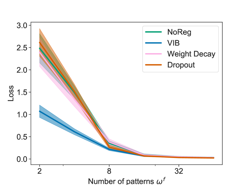
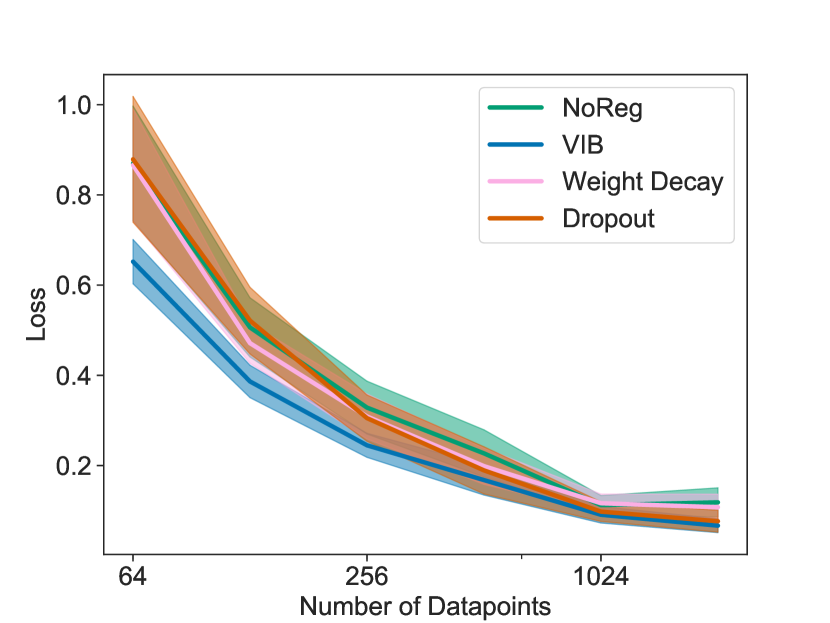
First we start in the supervised setting and show on a synthetic dataset that the vib is particularly strong at finding more general features in the low-data regime and in the presence of multiple signals with varying degrees of generality. Our motivation is that the low-data regime is commonly encountered in rl early on in training and many environments allow the agent to base its decision on a variety of features in the state, of which we would like to find the most general ones.

We generate the training dataset $\mathcal{D}_{\text{train}}=\{(c_{i},x_{i})\}_{i=1}^{N}$ with observations $x_{i}\in\mathbb{R}^{d_{x}}$ and classes $c_{i}\in\{1,\dots,n_{c}\}$. Each data point $i$ is generated by first drawing the class $c_{i}\sim\mathit{Cat}(n_{c})$ from a uniform categorical distribution and generating the vector $x_{i}$ by embedding the information about $c_{i}$ in two different ways $g^{c}$ and $f^{c}$ (see appendix B for details). Importantly, only $g^{c}$ is shared between the training and test set. This allows us to measure the model’s relative reliance on $g^{c}$ and $f^{c}$ by measuring the test performance (all models perfectly fit the training data). We allow $f^{c}$ to encode the information about $c_{i}$ in $\omega^{f}$ different ways. Consequently, the higher $\omega^{f}$, the less general $f^{c}$ is.

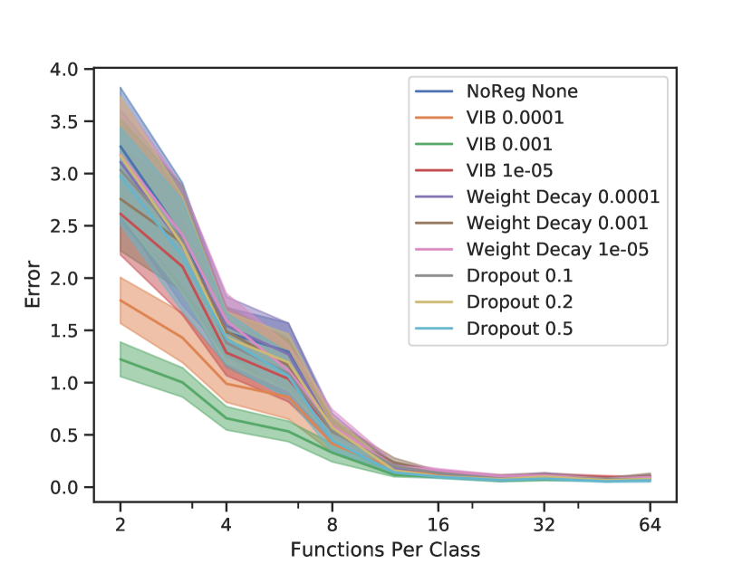
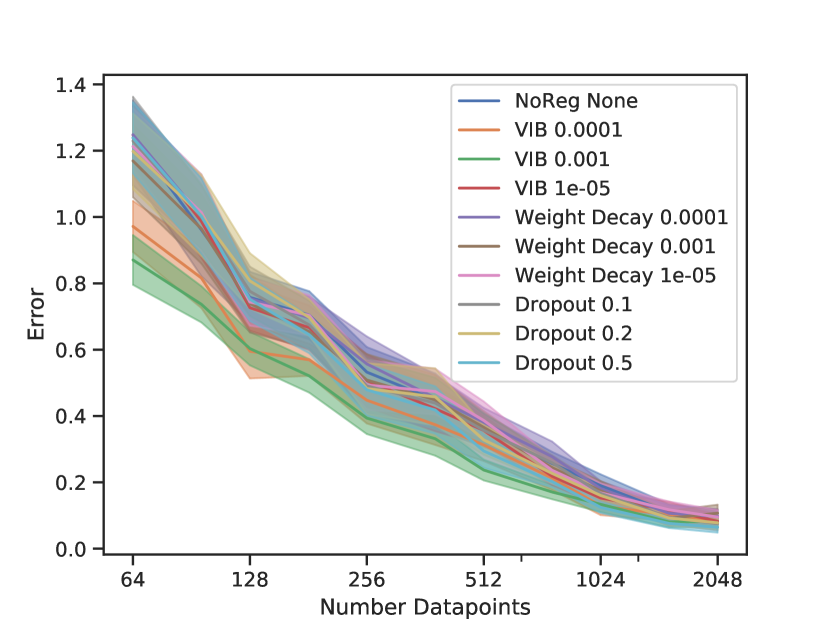
In fig. 1 we measure how the test performance of fully trained classification models varies for different regularization techniques when we i) vary the generality of $f^{c}$ and ii) vary the number of data-points in the training set. We find that most techniques perform comparably with the exception of the vib which is able to find more general features both in the low-data regime and in the presence of multiple features with only small differences in generality. In the next section, we show that this translates to faster training and performance gains in rl for our proposed algorithm ibac.

5.2 Multiroom

Figure 2: Left: Typical layout of the environment. The red triangle denotes the agent and its direction, the green full square is the goal, colored boxes are doors and grey squares are walls. Middle: Probability of finding the goal depending on level size for models trained on all levels. Shown are mean and standard error across 30 different seeds. Right: Mean and standard error over of the return of the same models averaged across all room sizes.

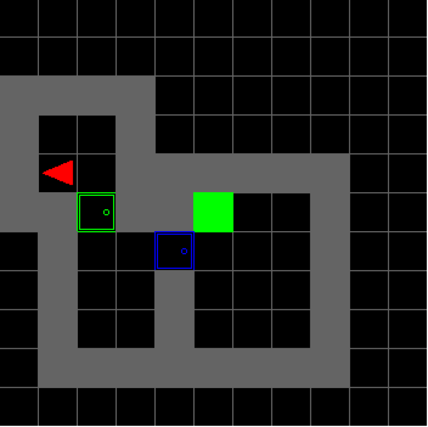
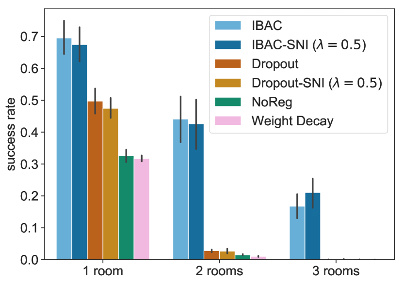
In this section, we show how ibac can help learning in rl tasks which require generalization. For this task, we do not distinguish between training and testing, but for each episode, we draw $m$ randomly from the full distribution over mdps $q(m)$. As the number of mdps is very large, learning can only be successful if the agent learns general features that are transferrable between episodes.

This experiment is based on [9]. The aim of the agent is to traverse a sequence of rooms to reach the goal (green square in fig. 2) as quickly as possible. It takes discrete actions to rotate $90\degree$ in either direction, move forward and toggle doors to be open or closed. The observation received by the agent includes the full grid, one pixel per square, with object type and object status (like direction) encoded in the 3 color channels. Crucially, for each episode, the layout is generated randomly by placing a random number of rooms $n_{r}\in\{1,2,3\}$ in a sequence connected by one door each.

The results in fig. 2 show that ibac agents are much better at successfully learning to solve this task, especially for layouts with more rooms. While all other fully trained agents can solve less than 3% of the layouts with two rooms and none of the ones with three, ibac-sni still succeeds in an impressive 43% and 21% of those layouts. The difficulty of this seemingly simple task arises from its generalization requirements: Since the layout is randomly generated in each episode, each state is observed very rarely, especially for multi-room layouts, requiring generalization to allow learning. While in the 1 room layout the reduced policy stochasticity of the sni agent slightly reduces performance, it improves performance for more complex layouts in which higher noise becomes detrimental. In the next section we will see that this also holds for the much more complex Coinrun environment in which sni significantly improves the ibac performance.

5.3 Coinrun

Figure 3: Left: Performance of various agents on the test environments. We note that ‘BatchNorm’ corresponds to the best performing agent in [11]. Furthermore, ‘Dropout-sni ($\lambda=1$)’ is similar to the Dropout implementation used in [11] but was previously not evaluated with weight decay and data augmentation. Middle: Difference between test performance and train performance (see fig. 7). Without standard deviation for readability. Right: Averaged approximate KL-Divergence between rollout policy and updated policy, used as proxy for the variance of the importance weight. Mean and standard deviation are across three random seeds.

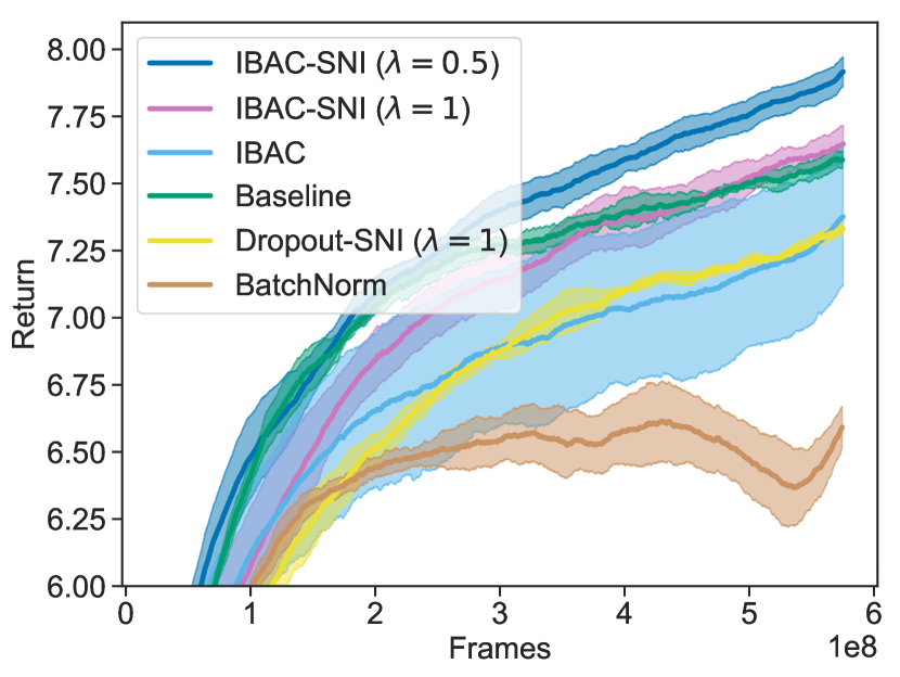
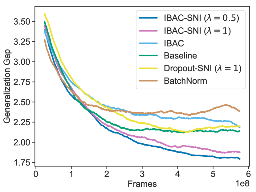
On the previous environment, we were able to show that ibac and sni help agents to find more general features and to do so faster. Next, we show that this can lead to a higher final performance on previously unseen test environments. We evaluate our proposed regularization techniques on Coinrun [11], a recently proposed generalization benchmark with high-dimensional observations and a large variety in levels. Several regularization techniques were previously evaluated there, making it an ideal evaluation environment for ibac and sni. We follow the setting proposed in [11], using the same 500 levels for training and evaluate on randomly drawn, new levels of only the highest difficulty.

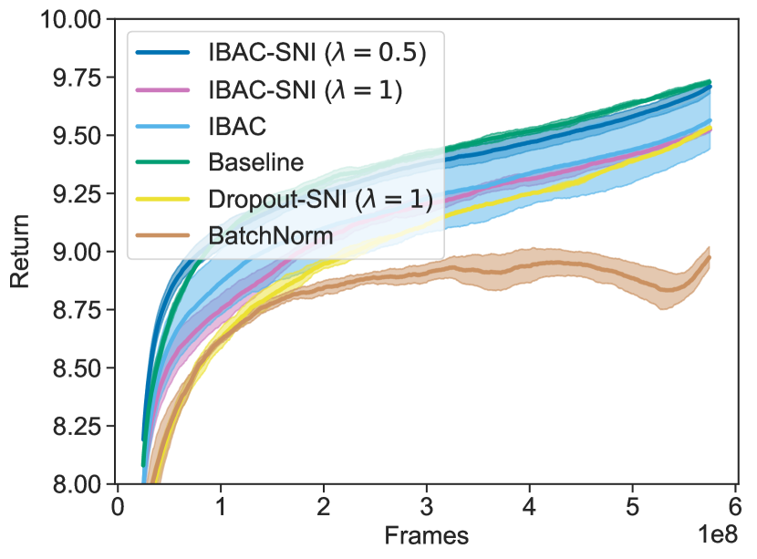
As [11] have shown, combining multiple regularization techniques can improve performance, with their best- performing agent utilizing data augmentation, weight decay and batch normalization. As our goal is to push the state of the art on this environment and to accurately compare against their results, fig. 3 uses weight decay and data-augmentation on all experiments. Consequently, ‘Baseline’ in fig. 3 refers to only using weight decay and data-augmentation whereas the other experiments use Dropout, Batch Normalization or ibac in addition to weight decay and data-augmentation. Results without those baseline techniques can be found in appendix D.

First, we find that almost all previously proposed regularization techniques decrease performance compared to the baseline, see fig. 3 (left), with batch normalization performing worst, possibly due to its unusual interaction with weight decay [56]. Note that this combination with batch normalization was the highest performing agent in [11]. We conjecture that regularization techniques relying on stochasticity can introduce additional instability into the training update, possibly deteriorating performance, especially if their regularizing effect is not sufficiently different from what weight decay and data-augmentation already achieve. This result applies to both batch normalization and Dropout, with and without sni, although sni mitigates the adverse effects. Consequently, we can already improve on the state of the art by only relying on those two non-stochastic techniques. Furthermore, we find that ibac in combination with sni is able to significantly outperform our new state of the art baseline. We also find that for ibac, $\lambda=0.5$ achieves better performance than $\lambda=1$, justifying using both terms in eq. 7.

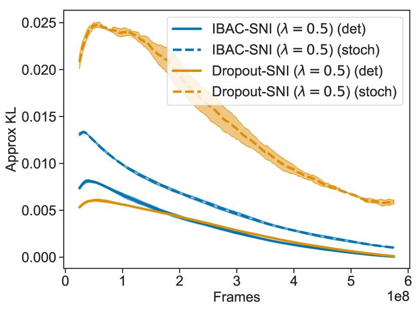
As a proxy for the variance of the off-policy correction term $\nicefrac{{\pi^{r}_{\theta}}}{{\pi_{\theta}}}$, we show in fig. 3 (right) the estimated, averaged KL-divergence between the rollout policy and the update policy for both terms, $\mathcal{G}_{\lx@glossaries@gls@link{acronym}{AC}{\leavevmode\textsc{ac}}}(\bar{\pi}_{\theta}^{r},\bar{\pi}_{\theta},\bar{V}_{\theta})$, denoted by ‘(det)’ and $\mathcal{G}_{\lx@glossaries@gls@link{acronym}{AC}{\leavevmode\textsc{ac}}}(\bar{\pi}_{\theta}^{r},\pi_{\theta},\bar{V}_{\theta})$, denoted by ‘(stoch)’. Because ppo uses data-points multiple times it is non-zero even for the deterministic term. First, we can see that using the deterministic version reduces the KL-Divergence, explaining the positive influence of $\mathcal{G}_{\lx@glossaries@gls@link{acronym}{AC}{\leavevmode\textsc{ac}}}(\bar{\pi}_{\theta}^{r},\bar{\pi}_{\theta},\bar{V}_{\theta})$. Second, we see that the KL-Divergence of the stochastic part is much higher for Dropout than for ibac, offering an explanation of why for Dropout relying on purely the deterministic part ($\lambda=1$) outperforms an equal mixing $\lambda=0.5$ (see fig. 6).

6 Related Work

Generalization in RL can take a variety of forms, each necessitating different types of regularization. To position this work, we distinguished two types that, whilst not mutually exclusive, we believe to be conceptually distinct and found useful to isolate when studying approaches to improve generalization.

The first type, robustness to uncertainty refers to settings in which the unobserved mdp $m$ influences the transition dynamics or reward structure. Consequently the current state $s$ might not contain enough information to act optimally in the current mdp and we need to find the action which is optimal under the uncertainty about $m$. This setting often arises in robotics and control where exact physical characteristics are unknown and domain shifts can occur [27]. Consequently, domain randomization, the injection of randomness into the environment, is often purposefully applied during training to allow for sim-to-real transfer [26, 55]. Noise can be injected into the states of the environment [50] or the parameters of the transition distribution like friction coefficients or mass values [3, 34, 60]. The noise injected into the dynamics can also be manipulated adversarially [29, 36, 39]. As the goal is to prevent overfitting to specific mdps, it also has been found that using smaller [40] or simpler [66] networks can help. We can also aim to learn an adaptive policy by treating the environment as partially observable Markov decision process (pomdp) [35, 60] (similar to viewing the learning problem in the framework of Bayesian RL [37]) or as a meta-learning problem [1, 10, 13, 43, 51, 57].

On the other hand, we distinguish feature robustness, which applies to environments with high-dimensional observations (like images) in which generalization to previously unseen states can be improved by learning to extract better features, as the focus for this paper. Recently, a range of benchmarks, typically utilizing procedurally generated levels, have been proposed to evaluate this type of generalization [4, 11, 19, 20, 21, 22, 32, 59, 63].

Improving generalization in those settings can rely on generating more diverse observation data [11, 42, 55], or strong, often relational, inductive biases applied to the architecture [23, 49, 61]. Contrary to the results in continuous control domains, here deeper networks have been found to be more successful [7, 11]. Furthermore, this setting is more similar to that of supervised learning, so established regularization techniques like weight decay, dropout or batch-normalization have also successfully been applied, especially in settings with a limited number of training environments [11]. This is the work most closely related to ours. We build on those results and improve upon them by taking into account the specific ways in which rl is different from the supervised setting. They also do not consider the vib as a regularization technique.

Combining rl and vib has been recently explored for learning goal-conditioned policies [14] and meta-RL [41]. Both of these previous works [14, 41] also differ from the ibac architecture we propose by conditioning action selection on both the encoded and raw state observation. These studies complement the contribution made here by providing evidence that the vib can be used with a wider range of rl algorithms including demonstrated benefits when used with Soft Actor-Critic for continuous control in MuJoCo [41] and on-policy A2C in MiniGrid and MiniPacMan [14].

7 Conclusion

In this work we highlight two important differences between supervised learning and rl: First, the training data is generated using the learned model. Consequently, using stochastic regularization methods can induce adverse effects and reduce the quality of the data. We conjecture that this explains the observed lower performance of Batch Normalization and Dropout. Second, in rl, we often encounter a noisy, low-data regime early on in training, complicating the extraction of general features.

We argue that these differences should inform the choice of regularization techniques used in RL. To mitigate the adverse effects of stochastic regularization, we propose Selective Noise Injection (sni)which only selectively injects noise into the model, preventing reduced data quality and higher gradient variance through a noisy critic. On the other hand, to learn more compressed and general features in the noisy low-data regime, we propose Information Bottleneck Actor Critic (ibac), which utilizes an variational information bottleneck as part of the agent.

We experimentally demonstrate that the vib is able to extract better features in the low-data regime and that this translates to better generalization of ibac in rl. Furthermore, on complex environments, sni is key to good performance, allowing the combined algorithm, ibac-sni, to achieve state of the art on challenging generalization benchmarks. We believe the results presented here can inform a range of future works, both to improve existing algorithms and to find new regularization techniques adapted to rl.

Appendix A Dropout with SNI

In order to apply sni to Dropout, we need to decide how to ‘suspend’ the noise to compute $\bar{\pi}_{\theta}$. While one could apply no dropout mask and scale the activations accordingly, we empirically found it to be better to instead sample one dropout mask and keep it fixed for all gradient updates using the thus collected data. This follows the implementation used in [11].

Appendix B Supervised Classification Task

Network architecture and hyperparameters

The network consist of a 1D-convolutional layer with 10 filters and a kernel size of 11 followed by two hidden, fully connected layers of size 1024 and 256 and the last layer which outputs $n_{c}$ logits. When the vib or Dropout are used, they are applied to the last hidden layer. We use a learning rate of $1e-4$. The relative weight for weight decay was $\lambda_{w}=1e-3$, which performed best out of $\{1e-2,1e-3,1e-4,1e-5\}$. For the vib we used $\beta=1e-3$, which performed best out of $\{1e-2,1e-3,1e-4,1e-5\}$. Lastly, For dropout we tested the dropout rates $p_{d}\in\{0.1,0.2,0.5\}$, out of which $0.2$ performed best. Our results were stable across a range of hyperparameters, see fig. 5.

Figure 4: Generation of the input data $x$: We embed the information about $c$ twice, once through $f^{c}$ and once through $g^{c}$. See text for details.

Data generation

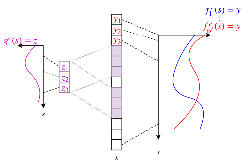
For each data-point, after drawing the class label $c_{i}$, we want to encode the information about $c_{i}$ in two ways, using the encoding functions $f^{c}$ and $g^{c}$ which use one of $\omega^{f}$ and $\omega^{g}$ different patterns to encode the information. The larger $\omega$ is, the less general the encoding is as it applies to fewer data-points. Note that there are $\omega$ different patterns per class.

We generate the patterns by first generating a set of random functions $\{f^{c}_{j}\}_{j=1}^{\omega^{f}}$ and $\{g^{c}_{j}\}_{j=1}^{\omega^{g}}$ by randomly drawing Fourier coefficients from $[0,1]$. Those functions are converted into vectors by evaluating them at $d_{x}$ sorted points randomly drawn from $[0,1]$. The resulting pattern-vectors for $f^{c}$ will have a dimension of $d_{x}$, whereas the ones for $g^{c}$ will be smaller, $d_{g}<d_{x}$.

To encode the information about $c_{i}$ we first choose one pattern from $\{f^{c}_{j}\}_{j}$ (slightly overloading notation between functions and pattern-vectors) and add some noise:

$$x^{\prime}_{i}=f^{c}_{j}+\epsilon_{i}\quad\text{where}\quad\epsilon\sim\mathcal{N}(0,\sigma_{\epsilon})\quad\text{and}\quad j\sim\mathit{Cat}(\omega^{f})$$ (13)

Next, to also encode the information about $c_{i}$ using $g^{c}$, we choose one of the $\omega^{g}$ patterns $\{g^{c}_{j}\}_{j}$ and replace a part of the vector $x^{\prime}_{i}$, which is possible because the $g^{c}$ patterns are shorter: $d_{g}<d_{x}$. The location of replacement is randomly drawn for each data-point, but restricted to a a set of $n_{g}$ possible locations which are also random, but kept fixed for the experiment and the same between training and testing set. The process is pictured in fig. 4.

By changing the number of possible locations $n_{g}$ and the strength of the noise added to $f^{c}$, $\sigma_{\epsilon}$,we can tune the relative difficulty of learning to recognize patterns $g^{c}$ and $f^{c}$, allowing us to find a regime where both can be found. Within this regime, our qualitative results were stable. We use $n_{g}=3$ and $\sigma_{\epsilon}=1$. Furthermore, we have for the dimension of of the observations $d_{x}=100$, and for the size of the patterns $g^{c}$ we have $d_{g}=20$. We use $n_{c}=5$ different classes.

Figure 5: Loss function (error) on test set. Same results as in main text, but for multiple hyperparameters. The qualitative results are stable under a wide range of hyperparameters.

Appendix C Multiroom

The observation space measures $11\times 11\times 3$ where the $3$ channels are used to encode object type and object features like orientation or ‘open/closed’ and ‘color’ for doors on each of the $11\times 11$ spatial locations (see fig. 2 for a typical layout for $n_{r}=3$).

The agent uses a 3-layer CNN with $16,32$ and $32$ filters respectively. All layers use a kernel of size $2$. After the CNN, it uses one hidden layer of size 64 to which ibac or Dropout are applied if they are used. Dropout uses $p_{d}=0.2$ and was tested for $\{0.1,0.2,0.5\}$. Both weight decay and ibac were tried with a weighting factor of $\{1e-3,1e-4,1e-5,1e-6\}$, with $1e-4$ performing best for weight decay and $1e-6$ performing best for ibac. The output of the hidden layer is fed into a value function head and the policy head.

We use a discount factor $\gamma=0.99$, a learning rate of $7e-4$, generalized value estimation with$\lambda_{\text{GAE}}=0.95$ [45], an entropy coefficient of $\lambda_{H}=0.01$, value loss coefficient $\lambda_{V}=0.5$, gradient clipping at $0.5$ [45], and ppo with the Adam optimizer [24].

Appendix D Coinrun

Architecture and Hyperparameters

We use the same architecture (’Impala’) and default policy gradient hyperparameters as well as the codebase (https://github.com/openai/coinrun) from the authors of [11] to ensure staying as closely as possible to their proposed benchmark.

Dropout and ibac where applied to the last hidden layer and both, as well as weight decay, were tried with the same set of hyperparameters as in Multiroom. The best performance was achieved with $p_{d}=0.2$ for Dropout and $1e-4$ for ibac and weight decay. Batch normalization was applied between the layers of the convolutional part of the network. Note that the original architecture in [11] uses Dropout also on earlier layers, however, we achieve higher performance with our implementation.

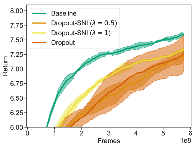
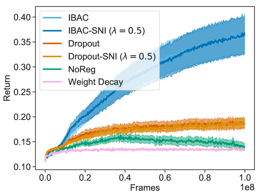
In fig. 6 (left) we show results for Dropout with and without sni and for $\lambda=1$ and $\lambda=0.5$. We find that $\lambda=1$ learns fastest, possible due to the high importance weight variance in the stochastic term in sni for $\lambda<1$ (see fig. 3 (right)). However, all Dropout implementations converge to roughly the same value, significantly below the ‘baseline’ agent, indicating that Dropout is not suitable for combination with weight decay and data augmentation.

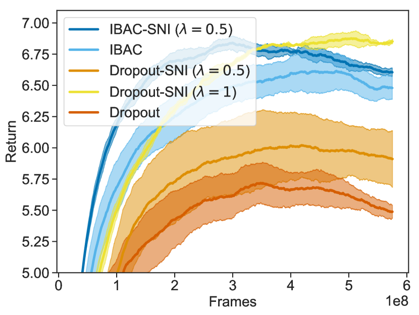
In fig. 6 (right) we show the test performance for ibac and Dropout with and without sni, without using weight decay and data-augmentation. Again, we can see that sni helps the performance. Interestingly, we can see that ibac does not prevent overfitting by itself (one can see the performance decreasing for longer training) but does lead to faster learning. Our conjecture is that it finds more general features early on in training, but ultimately overfits to the test-set of environments without additional regularization. This further indicates that it’s regularization is different to techniques such as weight decay, explaining why their combination synergizes well.

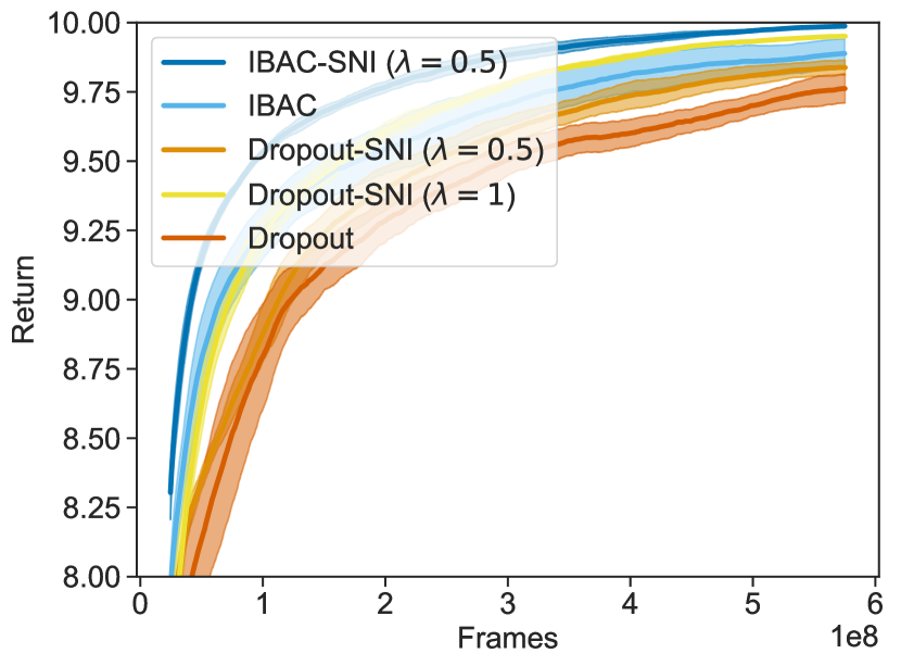
In fig. 7 we show the training set performance of our experiments.

Figure 6: Left: Comparison for different implementations of Dropout on the test environments. Right: Comparison of ibac and Dropout, with and without sni, without weight decay and data augmentation.

Figure 7: Training Performance with weight decay and data augmentation (left) and without (right)

References

- [1] Maruan Al-Shedivat, Trapit Bansal, Yura Burda, Ilya Sutskever, Igor Mordatch, and Pieter Abbeel. Continuous adaptation via meta-learning in nonstationary and competitive environments. In International Conference on Learning Representations, 2018.
- [2] Alexander A. Alemi, Ian Fischer, Joshua V. Dillon, and Kevin Murphy. Deep variational information bottleneck. In 5th International Conference on Learning Representations, ICLR 2017, Toulon, France, April 24-26, 2017, Conference Track Proceedings, 2017.
- [3] Rika Antonova, Silvia Cruciani, Christian Smith, and Danica Kragic. Reinforcement learning for pivoting task. arXiv preprint arXiv:1703.00472, 2017.
- [4] Edward Beeching, Christian Wolf, Jilles Dibangoye, and Olivier Simonin. Deep reinforcement learning on a budget: 3d control and reasoning without a supercomputer. CoRR, abs/1904.01806, 2019.
- [5] Mikhail Belkin, Daniel Hsu, Siyuan Ma, and Soumik Mandal. Reconciling modern machine learning and the bias-variance trade-off. arXiv preprint arXiv:1812.11118, 2018.
- [6] Marc G Bellemare, Yavar Naddaf, Joel Veness, and Michael Bowling. The arcade learning environment: An evaluation platform for general agents. Journal of Artificial Intelligence Research, 47:253–279, 2013.
- [7] Alon Brutzkus and Amir Globerson. Over-parameterization improves generalization in the XOR detection problem. CoRR, abs/1810.03037, 2018.
- [8] Devendra Singh Chaplot, Guillaume Lample, Kanthashree Mysore Sathyendra, and Ruslan Salakhutdinov. Transfer deep reinforcement learning in 3d environments: An empirical study. In NIPS Deep Reinforcemente Leaning Workshop, 2016.
- [9] Maxime Chevalier-Boisvert and Lucas Willems. Minimalistic gridworld environment for openai gym. https://github.com/maximecb/gym-minigrid, 2018.
- [10] Ignasi Clavera, Anusha Nagabandi, Ronald S. Fearing, Pieter Abbeel, Sergey Levine, and Chelsea Finn. Learning to adapt: Meta-learning for model-based control. CoRR, abs/1803.11347, 2018.
- [11] Karl Cobbe, Oleg Klimov, Chris Hesse, Taehoon Kim, and John Schulman. Quantifying generalization in reinforcement learning. In Proceedings of the 36th International Conference on Machine Learning, 2019.
- [12] Terrance DeVries and Graham W Taylor. Improved regularization of convolutional neural networks with cutout. arXiv preprint arXiv:1708.04552, 2017.
- [13] Yan Duan, John Schulman, Xi Chen, Peter L Bartlett, Ilya Sutskever, and Pieter Abbeel. Rl2: Fast reinforcement learning via slow reinforcement learning. arXiv preprint arXiv:1611.02779, 2016.
- [14] Anirudh Goyal, Riashat Islam, DJ Strouse, Zafarali Ahmed, Hugo Larochelle, Matthew Botvinick, Sergey Levine, and Yoshua Bengio. Infobot: Transfer and exploration via the information bottleneck. In International Conference on Learning Representations, 2019.
- [15] Peter Henderson, Riashat Islam, Philip Bachman, Joelle Pineau, Doina Precup, and David Meger. Deep reinforcement learning that matters. In Thirty-Second AAAI Conference on Artificial Intelligence, 2018.
- [16] Matteo Hessel, Joseph Modayil, Hado Van Hasselt, Tom Schaul, Georg Ostrovski, Will Dabney, Dan Horgan, Bilal Piot, Mohammad Azar, and David Silver. Rainbow: Combining improvements in deep reinforcement learning. In Thirty-Second AAAI Conference on Artificial Intelligence, 2018.
- [17] Elad Hoffer, Itay Hubara, and Daniel Soudry. Train longer, generalize better: closing the generalization gap in large batch training of neural networks. In Advances in Neural Information Processing Systems, pages 1731–1741, 2017.
- [18] Sergey Ioffe and Christian Szegedy. Batch normalization: Accelerating deep network training by reducing internal covariate shift. In International Conference on Machine Learning, pages 448–456, 2015.
- [19] Matthew Johnson, Katja Hofmann, Tim Hutton, and David Bignell. The malmo platform for artificial intelligence experimentation. In IJCAI, pages 4246–4247, 2016.
- [20] Arthur Juliani, Ahmed Khalifa, Vincent-Pierre Berges, Jonathan Harper, Hunter Henry, Adam Crespi, Julian Togelius, and Danny Lange. Obstacle tower: A generalization challenge in vision, control, and planning. CoRR, abs/1902.01378, 2019.
- [21] Niels Justesen, Ruben Rodriguez Torrado, Philip Bontrager, Ahmed Khalifa, Julian Togelius, and Sebastian Risi. Illuminating generalization in deep reinforcement learning through procedural level generation. arXiv preprint arXiv:1806.10729, 2018.
- [22] Yuji Kanagawa and Tomoyuki Kaneko. Rogue-gym: A new challenge for generalization in reinforcement learning. arXiv preprint arXiv:1904.08129, 2019.
- [23] Ken Kansky, Tom Silver, David A Mély, Mohamed Eldawy, Miguel Lázaro-Gredilla, Xinghua Lou, Nimrod Dorfman, Szymon Sidor, Scott Phoenix, and Dileep George. Schema networks: Zero-shot transfer with a generative causal model of intuitive physics. In Proceedings of the 34th International Conference on Machine Learning-Volume 70, pages 1809–1818. JMLR. org, 2017.
- [24] Diederik P. Kingma and Jimmy Ba. Adam: A method for stochastic optimization. In 3rd International Conference on Learning Representations, ICLR 2015, San Diego, CA, USA, May 7-9, 2015, Conference Track Proceedings, 2015.
- [25] Diederik P. Kingma and Max Welling. Auto-encoding variational bayes. In 2nd International Conference on Learning Representations, ICLR 2014, Banff, AB, Canada, April 14-16, 2014, Conference Track Proceedings, 2014.
- [26] Sylvain Koos, Jean-Baptiste Mouret, and Stéphane Doncieux. The transferability approach: Crossing the reality gap in evolutionary robotics. IEEE Transactions on Evolutionary Computation, 17(1):122–145, 2013.
- [27] Sergey Levine, Peter Pastor, Alex Krizhevsky, Julian Ibarz, and Deirdre Quillen. Learning hand-eye coordination for robotic grasping with deep learning and large-scale data collection. The International Journal of Robotics Research, 37(4-5):421–436, 2018.
- [28] Ping Luo, Xinjiang Wang, Wenqi Shao, and Zhanglin Peng. Towards understanding regularization in batch normalization. In International Conference on Learning Representations, 2019.
- [29] Ajay Mandlekar, Yuke Zhu, Animesh Garg, Li Fei-Fei, and Silvio Savarese. Adversarially robust policy learning: Active construction of physically-plausible perturbations. In 2017 IEEE/RSJ International Conference on Intelligent Robots and Systems (IROS), pages 3932–3939. IEEE, 2017.
- [30] Volodymyr Mnih, Adria Puigdomenech Badia, Mehdi Mirza, Alex Graves, Timothy Lillicrap, Tim Harley, David Silver, and Koray Kavukcuoglu. Asynchronous methods for deep reinforcement learning. In International conference on machine learning, pages 1928–1937, 2016.
- [31] Volodymyr Mnih, Koray Kavukcuoglu, David Silver, Alex Graves, Ioannis Antonoglou, Daan Wierstra, and Martin A. Riedmiller. Playing atari with deep reinforcement learning. CoRR, abs/1312.5602, 2013.
- [32] Alex Nichol, Vicki Pfau, Christopher Hesse, Oleg Klimov, and John Schulman. Gotta learn fast: A new benchmark for generalization in rl. arXiv preprint arXiv:1804.03720, 2018.
- [33] OpenAI. Openai five. https://blog.openai.com/openai-five/, 2018.
- [34] Charles Packer, Katelyn Gao, Jernej Kos, Philipp Krähenbühl, Vladlen Koltun, and Dawn Song. Assessing generalization in deep reinforcement learning. arXiv preprint arXiv:1810.12282, 2018.
- [35] Xue Bin Peng, Marcin Andrychowicz, Wojciech Zaremba, and Pieter Abbeel. Sim-to-real transfer of robotic control with dynamics randomization. In 2018 IEEE International Conference on Robotics and Automation (ICRA), pages 1–8. IEEE, 2018.
- [36] Lerrel Pinto, James Davidson, Rahul Sukthankar, and Abhinav Gupta. Robust adversarial reinforcement learning. In Proceedings of the 34th International Conference on Machine Learning-Volume 70, pages 2817–2826. JMLR. org, 2017.
- [37] Pascal Poupart, Nikos Vlassis, Jesse Hoey, and Kevin Regan. An analytic solution to discrete bayesian reinforcement learning. In Proceedings of the 23rd international conference on Machine learning, pages 697–704. ACM, 2006.
- [38] Martin L Puterman. Markov decision processes: discrete stochastic dynamic programming. John Wiley & Sons, 2014.
- [39] Aravind Rajeswaran, Sarvjeet Ghotra, Balaraman Ravindran, and Sergey Levine. Epopt: Learning robust neural network policies using model ensembles. In 5th International Conference on Learning Representations, ICLR 2017, Toulon, France, April 24-26, 2017, Conference Track Proceedings, 2017.
- [40] Aravind Rajeswaran, Kendall Lowrey, Emanuel V Todorov, and Sham M Kakade. Towards generalization and simplicity in continuous control. In Advances in Neural Information Processing Systems, pages 6550–6561, 2017.
- [41] Kate Rakelly, Aurick Zhou, Deirdre Quillen, Chelsea Finn, and Sergey Levine. Efficient off-policy meta-reinforcement learning via probabilistic context variables. In Proceedings of the 36th International Conference on Machine Learning, 2019.
- [42] Fereshteh Sadeghi and Sergey Levine. CAD2RL: real single-image flight without a single real image. In Robotics: Science and Systems XIII, Massachusetts Institute of Technology, Cambridge, Massachusetts, USA, July 12-16, 2017, 2017.
- [43] Tom Schaul, Daniel Horgan, Karol Gregor, and David Silver. Universal value function approximators. In International conference on machine learning, pages 1312–1320, 2015.
- [44] John Schulman, Sergey Levine, Pieter Abbeel, Michael Jordan, and Philipp Moritz. Trust region policy optimization. In International Conference on Machine Learning, pages 1889–1897, 2015.
- [45] John Schulman, Philipp Moritz, Sergey Levine, Michael I. Jordan, and Pieter Abbeel. High-dimensional continuous control using generalized advantage estimation. In 4th International Conference on Learning Representations, ICLR 2016, San Juan, Puerto Rico, May 2-4, 2016, Conference Track Proceedings, 2016.
- [46] John Schulman, Filip Wolski, Prafulla Dhariwal, Alec Radford, and Oleg Klimov. Proximal policy optimization algorithms. arXiv preprint arXiv:1707.06347, 2017.
- [47] Ohad Shamir, Sivan Sabato, and Naftali Tishby. Learning and generalization with the information bottleneck. Theoretical Computer Science, 411(29-30):2696–2711, 2010.
- [48] Nitish Srivastava, Geoffrey Hinton, Alex Krizhevsky, Ilya Sutskever, and Ruslan Salakhutdinov. Dropout: a simple way to prevent neural networks from overfitting. The Journal of Machine Learning Research, 15(1):1929–1958, 2014.
- [49] Mario Srouji, Jian Zhang, and Ruslan Salakhutdinov. Structured control nets for deep reinforcement learning. In International Conference on Machine Learning, pages 4749–4758, 2018.
- [50] Freek Stulp, Evangelos Theodorou, Jonas Buchli, and Stefan Schaal. Learning to grasp under uncertainty. In 2011 IEEE International Conference on Robotics and Automation, pages 5703–5708. IEEE, 2011.
- [51] Flood Sung, Li Zhang, Tao Xiang, Timothy Hospedales, and Yongxin Yang. Learning to learn: Meta-critic networks for sample efficient learning. arXiv preprint arXiv:1706.09529, 2017.
- [52] Richard S Sutton, David A McAllester, Satinder P Singh, and Yishay Mansour. Policy gradient methods for reinforcement learning with function approximation. In Advances in neural information processing systems, pages 1057–1063, 2000.
- [53] Naftali Tishby, Fernando C Pereira, and William Bialek. The information bottleneck method. arXiv preprint physics/0004057, 2000.
- [54] Naftali Tishby and Noga Zaslavsky. Deep learning and the information bottleneck principle. In 2015 IEEE Information Theory Workshop (ITW), pages 1–5. IEEE, 2015.
- [55] Josh Tobin, Rachel Fong, Alex Ray, Jonas Schneider, Wojciech Zaremba, and Pieter Abbeel. Domain randomization for transferring deep neural networks from simulation to the real world. In 2017 IEEE/RSJ International Conference on Intelligent Robots and Systems (IROS), pages 23–30. IEEE, 2017.
- [56] Twan van Laarhoven. L2 regularization versus batch and weight normalization. arXiv preprint arXiv:1706.05350, 2017.
- [57] Jane X. Wang, Zeb Kurth-Nelson, Dhruva Tirumala, Hubert Soyer, Joel Z. Leibo, Rémi Munos, Charles Blundell, Dharshan Kumaran, and Matthew Botvinick. Learning to reinforcement learn. CoRR, abs/1611.05763, 2016.
- [58] Shimon Whiteson, Brian Tanner, Matthew E Taylor, and Peter Stone. Protecting against evaluation overfitting in empirical reinforcement learning. In 2011 IEEE Symposium on Adaptive Dynamic Programming and Reinforcement Learning (ADPRL), pages 120–127. IEEE, 2011.
- [59] Marek Wydmuch, Michał Kempka, and Wojciech Jaśkowski. Vizdoom competitions: playing doom from pixels. IEEE Transactions on Games, 2018.
- [60] Wenhao Yu, Jie Tan, C. Karen Liu, and Greg Turk. Preparing for the unknown: Learning a universal policy with online system identification. In Robotics: Science and Systems XIII, Massachusetts Institute of Technology, Cambridge, Massachusetts, USA, July 12-16, 2017, 2017.
- [61] Vinicius Zambaldi, David Raposo, Adam Santoro, Victor Bapst, Yujia Li, Igor Babuschkin, Karl Tuyls, David Reichert, Timothy Lillicrap, Edward Lockhart, Murray Shanahan, Victoria Langston, Razvan Pascanu, Matthew Botvinick, Oriol Vinyals, and Peter Battaglia. Deep reinforcement learning with relational inductive biases. In International Conference on Learning Representations, 2019.
- [62] Amy Zhang, Nicolas Ballas, and Joelle Pineau. A dissection of overfitting and generalization in continuous reinforcement learning. arXiv preprint arXiv:1806.07937, 2018.
- [63] Amy Zhang, Yuxin Wu, and Joelle Pineau. Natural environment benchmarks for reinforcement learning. arXiv preprint arXiv:1811.06032, 2018.
- [64] Chiyuan Zhang, Samy Bengio, Moritz Hardt, Benjamin Recht, and Oriol Vinyals. Understanding deep learning requires rethinking generalization. In 5th International Conference on Learning Representations, ICLR 2017, Toulon, France, April 24-26, 2017, Conference Track Proceedings, 2017.
- [65] Chiyuan Zhang, Oriol Vinyals, Remi Munos, and Samy Bengio. A study on overfitting in deep reinforcement learning. arXiv preprint arXiv:1804.06893, 2018.
- [66] Chenyang Zhao, Olivier Siguad, Freek Stulp, and Timothy M Hospedales. Investigating generalisation in continuous deep reinforcement learning. arXiv preprint arXiv:1902.07015, 2019.