Parametrized ringdown spin expansion coefficients:
a data-analysis framework for black-hole spectroscopy with multiple events

Abstract

Black-hole spectroscopy is arguably the most promising tool to test gravity in extreme regimes and to probe the ultimate nature of black holes with unparalleled precision. These tests are currently limited by the lack of a ringdown parametrization that is both robust and accurate. We develop an observable-based parametrization of the ringdown of spinning black holes beyond general relativity, which we dub ParSpec (Parametrized Ringdown Spin Expansion Coefficients). This approach is perturbative in the spin, but it can be made arbitrarily precise (at least in principle) through a high-order expansion. It requires ${\cal O}(10)$ ringdown detections, which should be routinely available with the planned space mission LISA and with third-generation ground-based detectors. We provide a preliminary analysis of the projected bounds on parametrized ringdown parameters with LISA and with the Einstein Telescope, and discuss extensions of our model that can be straightforwardly included in the future.

I Introduction

Atomic spectroscopy revolutionized the quantum description of atomic interactions and paved the wave for quantum electrodynamics, through the precise measurements of the energy levels of the hydrogen atom LambShift . Black-hole (BH) spectroscopy 1980ApJ…239..292D ; Dreyer:2003bv ; Berti:2005ys – i.e., the measurement of the quasinormal modes (QNMs) of a BH Vishveshwara:1970cc ; Chandra ; Kokkotas:1999bd ; Ferrari:2007dd ; Berti:2009kk ; Konoplya:2011qq through gravitational wave (GW) ringdown observations – may play a similar major role to probe the gravitational interaction and fundamental physics in extreme conditions Berti:2015itd ; Barack:2018yly ; Berti:2018vdi ; Berti:2019xgr ; Sathyaprakash:2019yqt .

The post-merger ringdown signal from a remnant BH can be modeled as a superposition of damped sinusoids Kokkotas:1999bd ; Ferrari:2007dd ; Berti:2009kk , each defined by an oscillation frequency $\omega$ and a damping time $\tau$. Owing to the BH uniqueness and no-hair theorems Carter71 ; Hawking:1973uf ; Robinson ; Cardoso:2016ryw , the entire QNM spectrum of a spinning (Kerr) BH in general relativity (GR) is completely determined by the mass $M$ and spin $J=\chi M^{2}$ of the BH. (We use $G=c=1$ throughout.) Thus, measuring one frequency and damping time allows us to infer the mass and spin of a merger remnant from the ringdown signal only, whereas measuring more than two quantities (i.e., also subdominant modes) provides multiple independent null-hypothesis tests of GR Dreyer:2003bv ; Berti:2005ys ; Berti:2007zu ; Gossan:2011ha ; Meidam:2014jpa ; Bhagwat:2017tkm ; Baibhav:2017jhs ; Baibhav:2018rfk ; Brito:2018rfr ; Carullo:2018sfu . In addition, measuring also the amplitudes of multiple modes provides information about the intrinsic parameters of the progenitor binary Hughes:2019zmt ; Apte:2019txp ; Lim:2019xrb . These tests require high signal-to-noise ratio (SNR) in the ringdown Berti:2005ys ; Berti:2007zu and will become routinely available with the space mission LISA Audley:2017drz and with third-generation (3G) ground-based GW detectors (such as the proposed Einstein Telescope (ET) Punturo:2010zz and Cosmic Explorer Evans:2016mbw ), which are expected to detect several ringdown events per year with SNR in the hundreds to thousands, even from sources at cosmological distance Berti:2016lat .

The LIGO/Virgo Collaboration checked that the full inspiral-merger-ringdown waveform is consistent with GR by analyzing separately the lower-frequency signal emitted during the inspiral phase and the higher-frequency signal emitted during the late inspiral, merger and ringdown of the first event, GW150914 TheLIGOScientific:2016src . Separately fitting each of these signals to GR-based templates leads to two independent estimates of the mass and dimensionless spin of the remnant BH. An extension of this analysis to seven selected binary BH events found that the two estimates are compatible with each other within statistical errors of order $30\%$ (see Fig. 2 in LIGOScientific:2019fpa ). Recent work tried to better quantify the contribution of additional overtones to the high-frequency signal for GW150914. Adding at least one overtone is necessary to obtain ringdown estimates of the mass and spin of the remnant which are in agreement (at the $\sim 20\%$ level) with the values inferred by fitting the entire signal within GR Giesler:2019uxc ; Isi:2019aib (see also Berti:2007zu ; Baibhav:2017jhs ; Bhagwat:2019dtm ).

Going beyond these consistency tests requires modeling the BH ringdown beyond GR, for instance to perform a Bayesian model selection between GR and any proposed extension of the theory. This is a challenging task and, despite recent progress Barausse:2014tra ; Glampedakis:2017dvb ; Glampedakis:2017cgd ; Tattersall:2017erk ; Franciolini:2018uyq ; Cardoso:2019mqo ; McManus:2019ulj ; Glampedakis:2019dqh , all current attempts have significant limitations: they are based on particular classes of theories, they use geometric-optics approximations for the QNMs, or they neglect the spin of the remnant.

Working in the nonrotating limit is a major limitation, since the final spin of the merger remnant is typically high Buonanno:2006ui ; Berti:2007fi ; Berti:2008af ; Hofmann:2016yih . Including spin in current approaches is challenging, especially because the geometry of spinning BHs beyond GR is known only perturbatively or numerically (see e.g. Pani:2011gy ; Kleihaus:2011tg ; Ayzenberg:2014aka ; Maselli:2015tta ; Barausse:2015frm ; Herdeiro:2016tmi ; Cunha:2019dwb for specific examples and Berti:2015itd ; Herdeiro:2015waa ; Yagi:2016jml for reviews), which makes it very hard to compute the QNMs. In addition, there is in general no analog of the Teukolsky equation Teukolsky:1972my ; Teukolsky:1973ha ; Chandra beyond GR. In general the perturbation equations are not separable Pani:2013pma , and this requires the solution of an elliptic system of partial differential equations Dias:2015wqa or the extraction of QNM frequencies from numerical-relativity simulations of BH mergers Okounkova:2017yby ; Witek:2018dmd ; Okounkova:2019dfo ; Okounkova:2019zep .

In contrast to these major technical limitations, modeling the BH QNMs beyond GR is remarkably straightforward. In any extension of GR, the QNMs of a BH can be parametrized as Gossan:2011ha ; Meidam:2014jpa ; Carullo:2018sfu

$$\omega = \omega^{\rm Kerr}+\delta\omega\,,$$ (1)

$$\tau = \tau^{\rm Kerr}+\delta\tau\,,$$ (2)

where the frequency $\omega^{\rm Kerr}$ and damping time $\tau^{\rm Kerr}$ depend only on $M$ and $\chi$, whereas $\delta\omega$ and $\delta\tau$ are generic deviations. We consider a modified ringdown which deviates perturbatively from the Kerr case in GR, i.e. $\delta\omega\ll\omega^{\rm Kerr}$ and $\delta\tau\ll\tau^{\rm Kerr}$. These departures can be due to extra charges, a modified theory of gravity, environmental effects, etcetera, and we wish to develop a generic framework that can accommodate various special cases. GR corrections might affect the ringdown in two ways: by predicting a spinning BH other than Kerr Kleihaus:2011tg ; Ayzenberg:2014aka ; Barausse:2015frm ; Cardoso:2018ptl ; Yagi:2016jml ; Berti:2015itd ; Barack:2018yly ; Sathyaprakash:2019yqt , or (even if GR BHs are still solutions of the theory) by affecting the dynamics of the perturbations Barausse:2008xv ; Molina:2010fb ; Tattersall:2017erk ; Tattersall:2018map ; Tattersall:2018nve ; Tattersall:2019pvx . In both cases, the ringdown modes will acquire corrections proportional to the fundamental coupling constant(s) of the theory. There may be new classes of modes associated to extra polarizations, but they are unlikely to be significantly excited for GR deviations small enough to be compatible with existing observations Molina:2010fb ; Barausse:2014tra ; Blazquez-Salcedo:2016enn . For this reason they will not be considered in our analysis.

The above discussion suggests that a case-by-case analysis is impractical, and that parametrizing directly the observables (i.e., frequencies and damping times) is the most efficient way to perform ringdown tests (see e.g. Meidam:2014jpa ; Carullo:2018sfu ; Cardoso:2019mqo ; McManus:2019ulj for work in this direction). Similar observable-based approaches have been very successful to model weak-field effects Will:2014kxa and the inspiral Yunes:2009ke ; Agathos:2013upa .

In this paper we develop a scheme based on “Parametrized Ringdown Spin Expansion Coefficients” (ParSpec) which differs from related hierarchical approaches Isi:2019asy and mode-stacking proposals Yang:2017zxs . Its salients features are as follows:

• We expand the spectrum in a bivariate series in terms of the fundamental parameters (mass and spin) characterizing BH dynamics in GR.

• The expansion parameters take into account the fact that modifications of GR are suppressed by a (possibly dimensionful) coupling constant.

• Bayesian inference allows us to identify the most easily measurable expansion coefficients. By combining several observations, we can in principle map the deviation parameters to specific modified theories of gravity for which QNM spectra may be available. Since the third LIGO/Virgo observing run has been detecting BH mergers on a weekly basis, this approach holds the promise of allowing us to constrain several parameters (or identify deviations) as soon as the typical SNR of the observations becomes large enough.

The plan of the paper is as follows. In Section II we describe our parametrized framework. In Section III we illustrate the potential of the method by performing a statistical analysis on a representative catalog of merger events with LISA and 3G Earth-based detectors. In Sections IV and  V we compare our framework with previous work and discuss directions for future research.

II PARSPEC framework

Let us assume $i=1,\,\dots,\,N$ independent ringdown detections, for which $q$ QNMs are measured. In general $q$ depends on the source $i$, but for simplicity we shall consider a subset of all $N_{T}$ merger events for which the same number $q$ of QNMs passes a certain SNR threshold. Therefore $N$ is (in general) smaller than $N_{T}$, but this is not a major limitation, given the high event rates expected for future detectors.

In terms of a standard spheroidal-harmonics decomposition Berti:2009kk , and depending on the intrinsic parameters of the progenitor binary (mass ratio and spins), typically the most excited QNMs  are the fundamental modes with $l=m=2$, $l=m=3$, and $l=2$, $m=1$. For simplicity we will assume the subdominant mode to be $l=m=3$ for all $N_{T}$ sources; this assumption will be justified below. For a given $(l,m)$, the overtones are in general relevant for parameter estimation Leaver:1986gd ; Berti:2006wq ; London:2014cma ; Baibhav:2017jhs ; Giesler:2019uxc ; Isi:2019aib . However, the frequencies of different overtones are very similar and hard to resolve Berti:2005ys ; Bhagwat:2019dtm , and therefore it is hard to use them for direct BH spectroscopy. For this reason, in this paper we will not consider overtones.

	$l=2,m=2$		$l=3,m=3$		$l=2,m=1$
$n$	$w^{(n)}$	$t^{(n)}$	$w^{(n)}$	$t^{(n)}$	$w^{(n)}$	$t^{(n)}$
$0$	$0.3737$	$11.2407$	$0.5994$	$10.7871$	$0.3737$	$11.2407$
$1$	$0.1258$	$0.2522$	$0.2021$	$0.2276$	$0.0629$	$0.1261$
$2$	$0.0717$	$0.6649$	$0.1072$	$0.8238$	$0.0449$	$0.7710$
$3$	$0.0480$	$0.5866$	$0.0689$	$0.7353$	$0.0218$	$0.3821$
$4$	$0.0350$	$0.5797$	$0.0491$	$0.0685$	$0.0163$	$0.5565$

Table 1: Coefficients of the spin expansion for the QNMs $l=m=2$, $l=m=3$ and $l=2$, $m=1$ of a Kerr BH in GR, obtained from the numerical data in ringdown .

Rather than considering the corrections in Eqs. (1) and (2) as independent parameters, it is sensible and convenient to reduce the dimensionality of the parameter space by performing a spin expansion. To this aim, we parametrize each mode of the $i$-th source as

$$\omega_{i}^{(J)} = \frac{1}{M_{i}}\sum_{n=0}^{D}\chi^{n}_{i}w^{(n)}_{J}\left(1+\gamma_{i}\delta w^{(n)}_{J}\right)\,,$$ (3)

$$\tau_{i}^{(J)} = M_{i}\sum_{n=0}^{D}\chi^{n}_{i}t^{(n)}_{J}\left(1+\gamma_{i}\delta t^{(n)}_{J}\right)\,,$$ (4)

where $J=1,2,...,q$ labels the mode; $M_{i}$ and $\chi_{i}\ll 1$ are the detector-frame mass and spin of the $i$-th source, both measured assuming GR (see below); $D$ is the order of the spin expansion; $w^{(n)}_{J}$ and $t^{(n)}_{J}$ are the dimensionless coefficients of the spin expansion for a Kerr BH in GR (provided in Table 1 for a few representative modes); $\gamma_{i}$ are dimensionless coupling constants, which can depend on the source $i$ – see Eq. (6) below – but do not depend on the specific QNM; and $\delta w^{(n)}_{J}$ and $\delta t^{(n)}_{J}$ are “beyond-Kerr” corrections to the QNM frequencies. Crucially, the latter are universal dimensionless numbers that do not depend on the source. Any possible source dependence is parametrized through $\gamma_{i}$, as discussed below.

As customary in parametrized approaches, we focus on perturbative corrections by assuming $\gamma_{i}\delta w^{(n)}\ll 1$, $\gamma_{i}\delta t^{(n)}\ll 1$, and GR is recovered in the limit $\gamma_{i}\to 0$.

We remark that in the parametrization (3), (4), $M_{i}$ and $\chi_{i}$ are the BH masses (in the detector frame) and spins extracted assuming GR. In a non-GR theory, these are generally different from the actual BH masses and spins, $\bar{M}_{i}$, $\bar{\chi}_{i}$ (see Appendix A). Therefore, the coefficients $\gamma_{i}$, $\delta w^{(n)}_{J}$ and $\delta t^{(n)}_{J}$ also include the shift between $M_{i}$, $\chi_{i}$ and the physical masses and spins. Since $M_{i}$ and $\chi_{i}$ refer to the GR values of the detector-frame mass and spin of the $i$-th source, they can be computed either from the full inspiral-merger-ringdown waveform within GR or from a measurement of the $l=m=2$ mode with a standard GR ringdown template (without any assumption on the luminosity distance of the source). The remaining parameters in Eqs. (3) and (4) are discussed below for various special cases.

II.1 Special cases

Case I: scale-free corrections. The simplest parametrized beyond-Kerr correction corresponds to having $\gamma_{i}=\alpha$ for all sources, where $\alpha$ is a dimensionless coupling constant. Then $\alpha$ can be re-absorbed within $\delta w^{(n)}$ and $\delta t^{(n)}$, and (assuming that $M_{i}$ and $\chi_{i}$ are known within some parameter estimation uncertainty) we can parametrize the QNM spectrum beyond GR with

$${\cal P}=2(D+1)q$$ (5)

parameters, where $2(D+1)q$ is the total number of $\delta w^{(n)}$ and $\delta t^{(n)}$ parameters required if we consider $q$ modes up to order $D$ in the spin expansion.

Case II: single dimensionful coupling. A more general model consists of a single fundamental, dimensionful coupling constant $\alpha$ (the extension to multiple coupling constants is straightforward). Without loss of generality, we assume that $\alpha$ has mass dimensions $[\alpha]={\hat{M}}^{p}$, where $p$ is fixed by the theory (for $p=0$ we recover Case I above). Here ${\hat{M}}$ is the typical mass/length scale in the problem, which for a BH coincides with its mass in the source frame $M^{\rm s}$, as measured within GR (see Appendix A for a discussion). In this case, since the coefficients $\gamma_{i}$ are linear in the coupling, to leading order in our perturbative scheme

$$\gamma_{i}=\frac{\alpha}{(M_{i}^{\rm s})^{p}}=\frac{\alpha(1+z_{i})^{p}}{M^{p}_{i}}\,,$$ (6)

are small dimensionless couplings that depend on the theory, on the source mass in the detector frame $M_{i}$, and on the source redshift $z_{i}$. The redshift can be estimated from the luminosity distance of the source, which can be extracted from the amplitude of the inspiral waveform (assuming the standard cosmological model). We will consider $p$ as fixed (in modified theories of gravity it is typically an integer, or possibly a rational number) so that the number of parameters is the same as in Case I [cf. Eq. (5)]. Note that $\alpha$ can be again reabsorbed within $\delta w^{(n)}$ and $\delta t^{(n)}$, but $\alpha$ is dimensionful if $p\neq 0$ (and so are $\delta w^{(n)}$ and $\delta t^{(n)}$ after the rescaling).

Cases  I (i.e., $p=0$) and II include some of the best studied modified theories of gravity:

• $p=0$: theories with dimensionless couplings in the action include certain scalar-tensor theories, Einstein-Aether and Hořava gravity (to leading order) Barausse:2013nwa .

• $p=4$: this case includes Einstein-scalar-Gauss-Bonnet Mignemi:1992nt ; Yunes:2011we ; Pani:2011gy ; Maselli:2015tta ; Julie:2019sab and dynamical Chern-Simons gravity Yunes:2009hc ; Ayzenberg:2014aka ; Maselli:2017kic . In this case $\gamma_{i}=\beta^{2}/(M^{\rm s}_{i})^{4}$, where $\beta$ is the coupling constant in the action, which has dimensions of a length squared in geometrical units.

• $p=6$: this case corresponds (e.g.) to certain classes of effective field theories Cardoso:2018ptl .

As discussed in McManus:2019ulj , if different classes of gravitational perturbations are non-degenerate at order zero in the coupling parameter, the leading-order corrections to the QNM frequencies coming from ${\cal O}(\alpha)$ terms in the action are ${\cal O}(\alpha^{2})$. In this case, an operator with mass dimension $p/2$ in the action will lead to a correction $\alpha^{2}/M^{p}$ in the QNMs. In the case of degenerate spectra (e.g., for axial and polar gravitational perturbations) the leading-order corrections to the QNMs coming from ${\cal O}(\alpha)$ terms in the action are also ${\cal O}(\alpha)$. The special cases discussed above correspond to terms in the action with mass dimension $0$, $2$ and $3$, respectively.

Case III: individual charges. Since the $\gamma_{i}$’s appearing in Eq. (6) depend only on the fundamental coupling and the masses in the source frame, Cases  I and II encompass BHs with secondary hair, but not BHs with primary hair (corresponding to an extra charge which does not depend on the mass and spin of the BH). A simple example of BHs with primary hair are Kerr-Newman BHs, which are useful and well-studied toy models for beyond-Kerr BHs, and may be astrophysically significant in certain dark-sector scenarios Cardoso:2016olt . In the case of BHs with primary hair we have

$$\gamma_{i}=\frac{Q_{i}^{2}}{(M^{\rm s}_{i})^{2}}\,,$$ (7)

where $Q_{i}$ is the charge of the $i$-th source. The number of parameters necessary to parametrize the spectrum then becomes

$${\cal P}^{\prime}={\cal P}+N=2(D+1)q+N\,.$$ (8)

Our approach is perturbative by assumption (i.e. $\gamma_{i}\ll 1$). In the Kerr-Newman example, this means that it can only accommodate weakly charged BHs.

II.2 Detection strategies

In summary, we can parametrize the QNM spectrum beyond GR with ${\cal P}$ parameters in Cases I and II, and ${\cal P}^{\prime}$ parameters in Case III. On the other hand, in principle for $N$ sources and $q$ modes we have a certain number ${\cal O}$ of observables, which depend on whether we consider the ringdown only, or rather extract $M_{i}$ and $\chi_{i}$ from the full inspiral-merger-ringdown waveform using numerical relativity fits (see e.g. Healy:2014yta ) or analytical models.

Using the inspiral-merger-ringdown. In this case we measure the individual binary component properties from the inspiral-merger-ringdown waveform, and we use numerical-relativity fits in GR to evaluate the final masses (in the detector frame) and spins in GR, $M_{i}$ and $\chi_{i}$ ($i=1,...,N$). This procedure allows us to use only the $l=m=2$ QNM to perform BH spectroscopy: it is essentially an extension of inspiral-merger-ringdown consistency checks that allows for a non-GR template in the ringdown.

In this case, for $N$ sources and $q$ modes we would have

$${\cal O}=2N\times q$$ (9)

observables, i.e. the frequencies and damping times of $q$ modes. Then we need

$$N>\left\{\begin{array}[]{ll}D+1&{\rm Cases~{}I~{}and~{}II,}\\ \frac{2(D+1)q}{2q-1}&{\rm Case~{}III,}\end{array}\right.$$ (10)

in order to have more observables than parameters. In this case also $q=1$ is allowed, i.e. the detection of the $l=m=2$ mode for all sources is sufficient to perform the test. For the minimal case $q=1$ (detection of one mode for each source) we get

$$N\geq\left\{\begin{array}[]{ll}D+1&{\rm Cases~{}I~{}and~{}II,}\\ 2(D+1)&{\rm Case~{}III.}\end{array}\right.$$ (11)

Using the ringdown only. For $N$ sources and $q$ modes we have

$${\cal O}=2N\times q-2N=2N\times(q-1)$$ (12)

observables, namely the frequencies and damping times of $q$ modes minus $2N$ observables (the frequencies and damping times of the fundamental modes) which have been used to extract the GR masses and spin. By comparing ${\cal O}$ with the number of parameters (either ${\cal P}$ or ${\cal P}^{\prime}$), we need

$$N>\left\{\begin{array}[]{ll}\frac{q(1+D)}{q-1}&{\rm Cases~{}I~{}and~{}II,}\\ \frac{2(D+1)q}{2q-3}&{\rm Case~{}III,}\end{array}\right.$$ (13)

in order to have more observables than parameters. Note that this condition is never satisfied for $q=1$, as expected, since a single mode can only allow us to determine the masses and spins for each source. For the minimal case $q=2$ (i.e., we are detecting $2$ modes for each source) we get

$$N\geq\left\{\begin{array}[]{ll}2D+2&{\rm Cases~{}I~{}and~{}II,}\\ 4D+4&{\rm Case~{}III.}\end{array}\right.$$ (14)

Equation (13) implies $N\geq D+1$ in all cases in the limit $q\gg 1$, i.e. when we can detect several modes for each source. Note that in this case we need twice of the sources that we needed in the inspiral-merger-ringdown case [Eq. (11) above].

Minimum number of sources. When the relations (11) and (14) are saturated, $N$ is the minimum number of sources necessary to perform the test, whereas further sources will allow for multiple, independent tests. The minimum number of sources depends on the truncation order of the spin expansion.

In order to estimate the accuracy needed when we truncate the spin expansion, in Fig. 1 we compare numerical calculations of the QNM frequencies of a Kerr BH with their small-spin expansion at various truncation orders. For $D\geq 4$ (resp., $D\geq 5$) the errors are smaller than $1\%$ for both the frequency (top panel) and damping time (bottom panel) when $\chi<0.6$ (resp., $\chi<0.7$). Therefore a truncation order $D=4$ or $D=5$ should be sufficient to compute the modes with an accuracy always better than $1\%$ up to spin $\chi=0.7$. Reaching the same accuracy at $\chi=0.8$ will require $D\geq 7$.

Figure 1: Relative percentage errors between the exact $l=m=2$ QNM of a Kerr BH (obtained using data from Ref. ringdown ) and their small-spin expansion for various truncation orders (see Table 1) as a function of the BH spin (the value of $D$ is indicated in the legend).

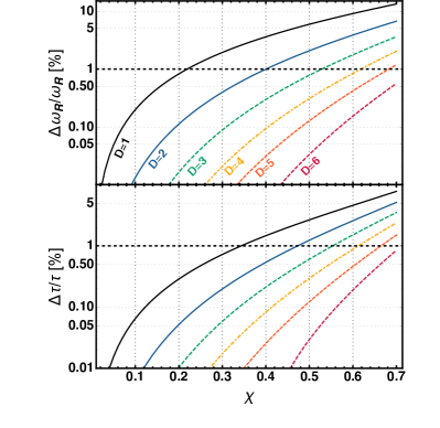
As a proof of principle of the ParSpec formalism, in the following we shall consider $D=4$ as a working assumption. We shall furthermore restrict to the simplest case (Case I), which minimizes the number of parameters and is more in line with existing parametrized tests, e.g. in the inspiral Will:2014kxa ; Yunes:2009ke ; Agathos:2013upa . Hence, we require $N\geq 5$ inspiral-merger-ringdown detections. Note that the minimum value of $N$ grows only linearly with $D$: even a very large spin expansion order (e.g., $D=10$) would require the same order of magnitude in terms of ringdown detections. Such a number of detections (even at large SNRs) may well be achievable with LISA and 3G detectors.

III Statistical analysis: Constraining the beyond-Kerr ringdown parameters

We use Eqs. (3)-(4), expanded up to fourth order in the spin, as templates to interpret the observed frequencies and damping times. We assume the true $(\omega_{i},\tau_{i})$ to correspond to a Kerr BH in GR, i.e. we assume the “true” beyond-Kerr parameters $\delta w^{(n)}$ and $\delta t^{(n)}$ to be zero.

Our goal is to reconstruct the probability distribution of the beyond-Kerr parameters. We consider either $q=1$ or $q=2$, i.e. either one or two modes detected for each of the $N$ sources. The purpose of this analysis is to compute the minimum value of the deformation parameters $\delta w^{(n)}$ and $\delta t^{(n)}$ which yield a ringdown observation consistent with GR. We consider a ground-based 3G detector (ET in the so called ET-D configuration Hild:2009ns ) and the planned space mission LISA Audley:2017drz as representatives of our best near-future chances to carry out BH spectroscopy over a large mass range Berti:2016lat ; Maselli:2017kvl .

Each source ($i=1,2,...,N$) provides frequencies and damping times $(\omega^{(J)}_{i,\,\text{obs}},\tau^{(J)}_{i,\,\text{obs}})$ for $J=1,\ldots,q$ modes, with associated parameter estimation errors $\sigma[{\omega_{i}^{(J)}}]$ and $\sigma[{\tau_{i}^{(J)}}]$ and correlations coefficients.

The values of $\omega^{(J)}_{i,\,\text{obs}}$ and $\tau^{(J)}_{i,\,\text{obs}}$ injected in our analysis are computed as follows. We consider the merger remnant of $N$ binary coalescences. The $2N$ masses of the binary components are drawn from a log-flat distribution between $[5,95]M_{\odot}$ for stellar-origin BHs, and from a uniform distribution within $[10^{6},10^{7}]M_{\odot}$ for massive BHs. For stellar-origin BHs we also require that $m_{1}+m_{2}<100M_{\odot}$ alLIGOScientificCollaborationandVirgoCollaboration:2018cn ; Belczynski:2016jno . In both mass ranges the spins are sampled from a uniform distribution $\in[-1,1]$. For illustration, we fix the source distance by choosing the SNR of the first ringdown mode to be $10^{2}$ for ET and $10^{3}$ for LISA, respectively. We then compute the mass and the spin of the final BH formed after merger using semianalytical relations based on numerical relativity simulations in GR Healy:2014yta (as discussed in Sec. II, these are the mass and spin that the final BH would have if GR is the correct theory of gravity). Given the final mass $M_{i}$ and spin $\chi_{i}$ ($i=1\ldots N$), we compute the errors on the modes through a Fisher-matrix approach. Following Berti:2006jo , we roughly estimate the energy in the secondary mode to be $10\%$ of the $l=m=2$ mode energy for all sources. The main purpose of these choices is to test our data-analysis framework, and we plan to implement more astrophysically realistic models in future work.

We use a Bayesian approach to sample the probability distributions $\mathbold{P}$ of the model parameters $\vec{\theta}$ for a given set of ringdown observations $\vec{d}$. By Bayes’ theorem $\mathbold{P}(\vec{\theta}|\vec{d})\propto\mathcal{L}(\vec{d}|\vec{\theta})\mathbold{P}_{0}(\vec{\theta})$, where $\mathcal{L}(\vec{d}|\vec{\theta})$ is the likelihood function and $\mathbold{P}_{0}(\vec{\theta})$ is the prior on the parameters. For each event, the likelihood function is chosen to be Gaussian:

$${\cal L}_{i}(\vec{d}|\vec{\theta})={\cal N}(\vec{\mu}_{i},\Sigma_{i})\,,$$ (15)

where the vector $\vec{\mu}_{i}$ depends on the difference between the observed $J=1,\ldots q$ modes and the parametrized templates (3)-(4):

$$\vec{\mu}_{i}=(\vec{\mu}_{i}^{(1)},\cdots,\vec{\mu}_{i}^{(q)})^{T}\,,$$ (16)

where each $\vec{\mu}_{i}^{(J)}$ is a two-component vector

$$\vec{\mu}_{i}^{(J)}=\begin{pmatrix}\omega^{(J)}_{i}-\omega^{(J)}_{i,\,\text{obs}}\\ \tau^{(J)}_{i}-\tau^{(J)}_{i,\,\text{obs}}\end{pmatrix}\ ,$$ (17)

and $\Sigma_{i}$ is the covariance matrix that includes errors and correlations between the frequencies and damping times measured for the $i$-th source. Under our assumptions the observed QNMs correspond to different values of $l$ and $m$, i.e. they are “quasi-orthonormal” in the terminology of Ref. Berti:2005ys . As a consequence the covariance matrix $\Sigma_{i}={\rm diag}(\Sigma^{(1)}_{i}\ldots\Sigma^{(q)}_{i})$ is block-diagonal with each block corresponding to the $J$-th mode, and the likelihood function can be written as a product of Gaussian distributions:

$${\cal N}(\vec{\mu}_{i},\Sigma_{i})=\prod_{J=1}^{q}{\cal N}(\vec{\mu}^{(J)}_{i},\Sigma^{(J)}_{i})\ .$$ (18)

Moreover, given $N$ independent BH detections, the combined likelihood function of the ParSpec parameters can be further factorized as

$${\cal L}(\vec{d}|\vec{\theta})=\prod_{i=1}^{N}{\cal L}_{i}(\vec{d}|\vec{\theta})=\prod_{i=1}^{N}\prod_{J=1}^{q}{\cal N}(\vec{\mu}^{(J)}_{i},\Sigma^{(J)}_{i})\ .$$ (19)

The full posterior is obtained through a Markov chain Monte Carlo (MCMC) method based on the Metropolis-Hastings algorithm Gilks:1996 , in which the proposal matrix is updated through a Gaussian adaptation which enhances the convergence to the target distribution 1085030 ; 5586491 . For each dataset we compute $4$ chains of $5\times 10^{6}$ points, with a thinning factor of $0.02$ to reduce the correlation between the samples. We discard $10\%$ of the initial points as a burn in.

The beyond-Kerr dimensionless parameters $\vec{\theta}=\{\delta w_{i}^{(J)},\delta t_{i}^{(J)}\}$ are sampled by assuming flat distributions within the interval $[-0.5,0.5]$. Moreover, for simplicity we assume the parameter $p$ associated with the mass dimension of the coupling to be $p=0$. We defer a more detailed investigation for different values of $p$ to future works. We remark that when $p>0$ the dimensionless coupling $\gamma_{i}=\alpha/M^{p}$ is much smaller for massive BH mergers, and therefore we expect QNM frequency corrections for LISA sources to be much smaller than those for stellar-origin BHs.

Figure 2: Posterior distributions for the beyond-Kerr ringdown parameters $\delta w_{1}^{(0)}$ and $\delta t_{1}^{(0)}$ inferred through the analysis of the $l=m=2$ fundamental QNM for ET, assuming $D=0$ and $q=1$. BH masses and spins are estimated from the inspiral-merger-ringdown signal. Colors correspond to different numbers of detections $N$.

III.1 Projected constraints with ET

III.1.1 Nonspinning black holes, one mode ($D=0$, $q=1$)

As a first case study we consider nonrotating BHs, i.e. we assume that $D=0$ in the spin expansion of the parametrized templates (3) and (4). If only the $l=m=2$ mode is detected for each source ($q=1$), the number of ParSpec parameters to constrain reduces to $\delta w_{1}^{(0)}$ and $\delta t_{1}^{(0)}$. We also focus on the first strategy discussed in Sec. II.2, i.e. we assume that the BH masses and spins are measured using the full inspiral-merger-ringdown signal. Then the minimum number of events required to perform our test is $N_{\rm min}=D+1=1$.

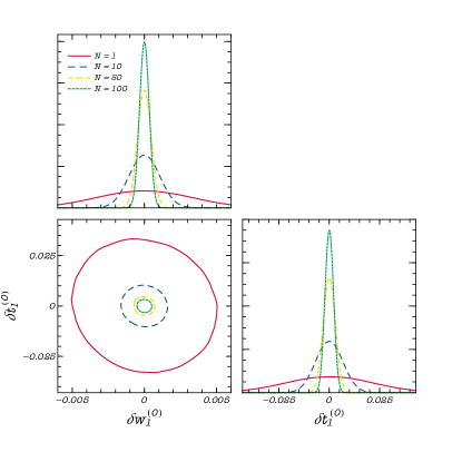
The top and right panels of Fig. 2 show the inferred marginalized distributions of the two ParSpec parameters as a function of the number $N$ of stellar mass sources detected by ET. The posteriors are peaked around zero and, as expected, they become narrower as $N$ grows. In the most optimistic case we consider ($N=100$) we find $|\delta w_{1}^{(0)}|\lesssim 5.4\times 10^{-4}$ and $|\delta t_{1}^{(0)}|\lesssim 3.4\times 10^{-3}$ at 90% confidence level. Since the distributions are nearly symmetrical around the peak, we can define their width as half of the corresponding confidence interval: $\sigma^{i}_{90}=1/2(\theta_{i}^{\rm max}-\theta_{i}^{\rm min})$, where $\theta_{i}^{\rm min}$ and $\theta_{i}^{\rm max}$ correspond to the values of the $i$-th parameter such that

$$\int_{\theta_{i}^{\rm min}}^{\theta_{i}^{\rm max}}\mathbold{P}(\theta_{i})d\theta_{i}=0.9$$ (20)

for the marginalized posterior. By fitting $\sigma^{i}_{90}$ as a function of $N$, we find that it scales like $\sim N^{-1/2}$ to a very good approximation. The contour plots in the bottom-left panel of Fig. 2 show $90\%$ confidence intervals for the 2D joint distribution of the two parameters, and they show that the parameters are almost completely uncorrelated.

III.1.2 Nonspinning black holes, two modes ($D=0$, $q=2$)

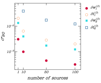
Our approach can accommodate an arbitrary number of modes. As a slightly more complex scenario, we still set $D=0$ but we now consider the observation of the primary ($l=m=2$) and secondary ($l=m=3$) QNM for each BH (i.e., $q=2$), thus doubling the number of parameters that we wish to constrain. Figure 3 shows the width $\sigma$ of the sampled posteriors as a function of $N$. The smallest values of $\sigma$ (i.e., the strongest bounds) correspond to the frequency corrections $\delta w^{(0)}_{1}$ and $\delta w^{(0)}_{2}$ of the primary and secondary mode, respectively. The widths are larger for corrections to the damping times ($\delta t^{(0)}_{1}$ and $\delta t^{(0)}_{2}$), which are typically harder to measure. Most importantly, Figure 3 shows that some of the ParSpec parameters can become measurable by increasing the number of observations $N$: for example, for $N=1$ the marginalized distribution of $\delta t_{2}^{(0)}$ is flat within the allowed range of values, and hence unconstrained by the data, but this quantity can be constrained for larger values of $N$. As in the $q=1$ case considered above, we find that the width of all parameters scales as $\sim N^{-1/2}$ to a very good approximation when the number of sources is large enough (typically of the order of $N\sim 100$).

Figure 3: 90% confidence intervals $\sigma_{90}$ for the posterior distributions of the parameters $\delta w$ and $\delta t$ of the first and second mode, as a function of the number of sources analysed and considering ET. We consider the case of nonrotating BHs, i.e. $D=0$, assuming that frequencies and damping times are measured through the inspiral-merger-ringdown signal. Only measurable parameters are shown.

Figure 4: 90% confidence intervals $\sigma_{90}$ of the beyond-Kerr ringdown spin coefficients considering GR modifications up to fourth order in rotation ($D=4$) as a function of the number of sources $N$ observed by ET. Top and bottom panels refer to $q=1$ and $q=2$, respectively. Only measurable parameters are shown.

Figure 5: Same as Fig. 4, but for massive BHs observed by LISA.

Figure 6: Comparison between the posteriors of some of the ParSpec parameters obtained for ET and LISA assuming spinning corrections with $D=4$ for $N=100$ sources. The probability distribution refers to the same dataset shown in the top panel of Fig. 5.

III.1.3 Spinning black holes ($D=4$, $q=1$ and $q=2$)

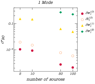
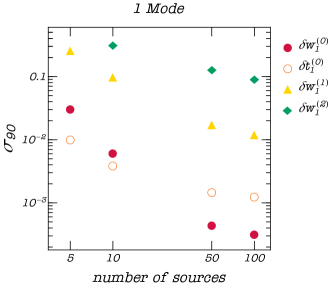
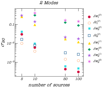
We can turn to the more realistic scenario of spinning BHs. We truncate the expansion at $D=4$, so that modes in GR are estimated with an accuracy better than $1\%$ up to spins $\chi\sim 0.6$ (see Fig. 1). Results for ET observations with $q=1$ and $q=2$ are shown in the top and bottom panels of Fig. 4, respectively.

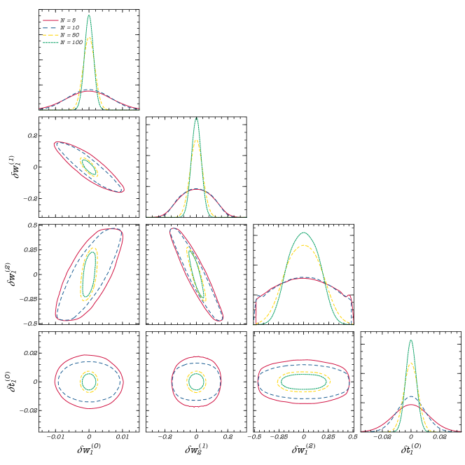
Consider first $q=1$ (top panel). Even with a large number of detections $N$, only some of the parameters are measurable. In general we can constrain with good accuracy the first three $\delta w_{1}^{(n)}$’s, i.e. GR deviations up to quadratic order in the spin ($n=0,\,1,\,2$). By contrast, only the non-spinning correction $\delta t_{1}^{(0)}$ to the damping times is bounded by the data.

Note however that $\delta w_{1}^{(2)}$ becomes measurable only for $N\gtrsim 50$. Moreover the posterior of the coefficients proportional to the BH’s angular momentum are more than one order of magnitude wider than the posterior of their nonspinning counterparts. For completeness, in Appendix B we show the corner plot for the marginalized and joint posterior distributions of the measurable ParSpec parameters for $q=1$. The spin-dependent frequency corrections show a correlation which generally decreases with $N$, while $\delta t_{1}^{(0)}$ is typically uncorrelated with the other coefficients.

The $q=2$ case (bottom panel of Fig. 4) is very similar: the width of the posteriors inferred through the MCMC decreases with $N$. The hierarchy among the beyond-Kerr parameters is also the same as in the single-mode case: zero-order (nonspinning) terms are best constrained, followed by corrections that are of low order in rotation. Remarkably, with $N=100$ sources we can put tight upper bounds on the coefficient of the secondary mode, with $|\delta w_{2}^{(0)}|\lesssim 7\times 10^{-3}$ $|\delta w_{2}^{(1)}|\lesssim 10^{-1}$ and $|\delta t_{2}^{(0)}|\lesssim 2\times 10^{-2}$.

These results can be straightforwardly adapted to the second detection strategy outlined in Sec. II.2. In this case we assume that for each observation we extract two QNMs from the postmerger GW signal, using the frequency and damping time of the fundamental mode to determine the mass and the spin of the source. This scenario is comparable to the single-mode case described above, but now we inject into the MCMC the subdominant QNM, which has lower SNR. Therefore we expect that the bounds shown in Fig. 3 and in the top panel of Fig. 4 would worsen by roughly one order of magnitude.

III.2 Projected constraints with LISA

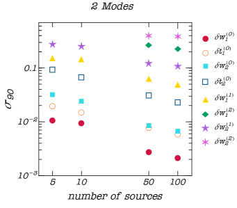
We now perform a similar Bayesian analysis for LISA QNM observations of massive BH binary mergers. For nonrotating BHs ($D=0$) the reconstructed posteriors are nearly a factor of ten tighter than the corresponding distributions for ET. This is somehow expected, since the parameters are nearly uncorrelated and the inference is dominated by the SNR of the detections (which we assumed to be one order of magnitude larger for LISA than for ET).

Figure 5 shows the width of the posteriors for spinning BHs with spin corrections up to $D=4$ and $q=1$ (top panel) or $q=2$ (bottom panel). The values of the upper bounds on the ParSpec parameters are in qualitative agreement with those obtained for ET in Fig. 4.

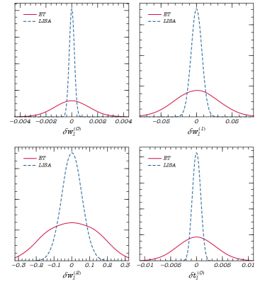
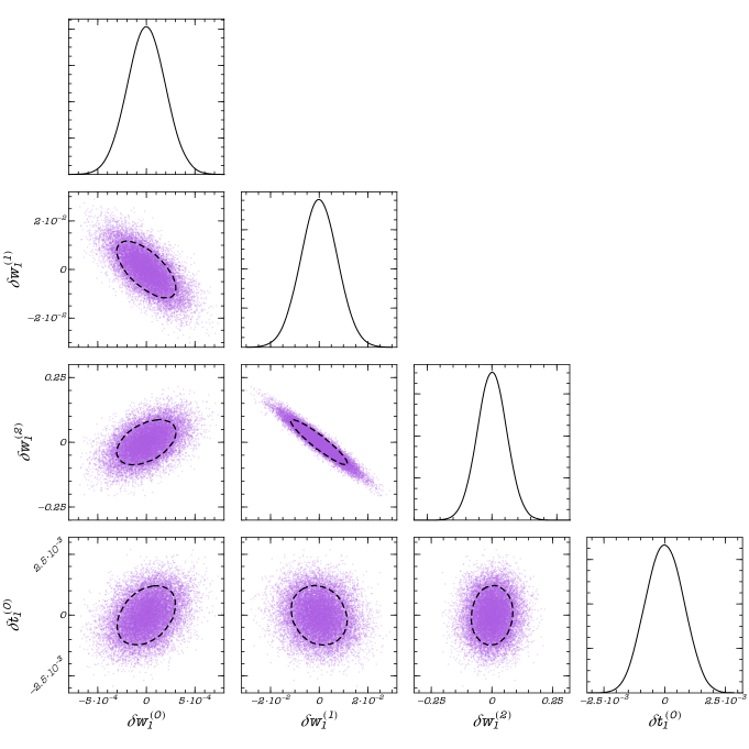
To facilitate comparisons, in Fig. 6 we show the posterior distributions inferred from a sample of $N=100$ observations with ET and LISA, assuming $q=1$. At least in the case of scale-free corrections considered in this work ($p=0$), LISA constraints are more stringent. For the best constrained parameters, the $90\%$ confidence intervals with LISA are $|\delta w_{1}^{(0)}|\lesssim 3.2\times 10^{-4}$ ($|\delta t_{1}^{(0)}|\lesssim 1.3\times 10^{-3}$), which are smaller than the corresponding values obtained for ET by a factor $\sim 6$ ($\sim 5$). For the upper bounds on the spinning coefficients we get $|\delta w_{1}^{(1)}|\lesssim 1.2\times 10^{-2}$ and $|\delta w_{1}^{(2)}|\lesssim 9.3\times 10^{-2}$ which are $\sim 4$ and $\sim 3$ times smaller than those inferred by ET. The corner plot in Fig. 8 of Appendix B shows the complete set of marginalized and joint distributions derived for such parameters. As already discussed in Sec. III.1, the coefficients $\delta w_{i}^{({J)}}$ that modify the mode’s frequencies are all correlated to each other, while the correction to the damping time is almost decoupled from the other parameters.

The two-mode analysis ($q=2$) follows the same trend. Moreover, comparing the bottom panels of Figs. 4 and 5 we note that – unlike ET – LISA will be able to constrain possible deviations from the primary and secondary modes with comparable accuracy.

IV Possible extensions

In this work we have presented a data-analysis framework (that we dub ParSpec ) and performed a preliminary analysis. Here we discuss several interesting extensions that should be explored in the future.

In our proof-of-principle data-analysis demonstration we consider only scale-free corrections, i.e. $p=0$. The extension to different values of $p$ (and hence to dimensionful couplings) is technically straightforward, but introducing a scale inevitably makes certain sources more relevant than others. Specifically, for a coupling parameter $\alpha$ with mass dimension $p$, sources with (source-frame) mass $M^{s}$ such that $\alpha/(M^{s})^{p}\sim 0.1$ will contribute the most, whereas sources with $\alpha/(M^{s})^{p}\ll 1$ will be irrelevant for the analysis. We could simply consider only the subset of events such that $\alpha/(M^{s})^{p}$ is larger than a fixed threshold. Overall, this would require more detections.

The assumption that our “true” signal is the standard ringdown within GR allows us to put at most upper bounds on the beyond-Kerr ringdown parameters, but we can search directly for GR deviations by writing the beyond-Kerr ringdown parameters explicitly for a given theory. As an extension, it would be interesting to consider a particular non-GR theory and to recover the ringdown signal in this theory with a standard GR ringdown template, in order to quantify systematic errors Vallisneri:2013rc .

Additional “branches” of the QNM spectrum which are not perturbatively close to the Kerr spectrum are expected in virtually any extension of GR, although they might be excited with small amplitude (see e.g. Molina:2010fb ; Blazquez-Salcedo:2016enn ; Tattersall:2017erk ; Okounkova:2017yby ; Witek:2018dmd ; Okounkova:2019dfo ). To leading order, the extra modes coincide with the corresponding QNMs of a Kerr BH in GR: for example, extra scalar (vector) degrees of freedom can give rise to standard scalar (vector) QNMs in the gravitational waveform, with amplitude proportional to the coupling parameter of the theory Molina:2010fb ; Blazquez-Salcedo:2016enn ; Tattersall:2017erk ; Witek:2018dmd . Our formalism can accommodate extra QNMs, which can be parametrized with Eqs. (3)–(4) with $\gamma_{i}=0$ by setting $w^{(n)}$ and $t^{(n)}$ to match the corresponding values for the (scalar, vector, etcetera) QNMs of a Kerr BH in GR (but see McManus:2019ulj for possible complications arising when different perturbations are coupled to each other).

Some theories of gravity may have multiple coupling constants, rather than the single perturbative parameter considered here. It is straightforward to extend our formalism to this case.

Our spin expansion is necessary to parametrize the ringdown in terms of a set of constant coefficients (as opposed to functions of the spin). The resulting systematic errors can be reduced by considering higher-order expansions than the $D=4$ case considered here. To check the impact of the truncation order, we have also considered a spin expansion truncated at $D=6$. In our tests, the posterior distribution of the measurable parameters did not change significantly relative to the $D=4$ case.

An obvious and important extension of our work is to compute rates for both 3G and LISA sources using more realistic astrophysical models. In this preliminary analysis we have assumed $10-100$ events at ${\rm SNR}\sim 100$ ($\sim 1000$) for ET (LISA), corresponding to nearby sources. It is important to estimate whether these estimates are realistic. Since we select only large-SNR sources, which are generally the closest ones, we have neglected the source redshift. Even the closest LISA ringdown sources may have nonnegligible redshift, and therefore cosmological effects should be included in a more refined analysis.

We assume that two different angular modes are detected for each sources. The extension to multiple angular modes is straightforward, and in general it should lead to stronger constraints. Likewise, in realistic scenarios not only the amplitude of the secondary mode, but also its nature will depend on the binary parameters (mass ratio and spins): in general the second most exited mode will correspond to $l=m=3$ only for a subset of sources, whereas the mode with $l=2$, $m=1$ and $l=m=4$ may be dominant for others. Future work should extend our parameter estimation strategy to the case of multiple, source-dependent secondary modes.

For any given $(l,\,m)$ we consider only the fundamental mode, neglecting the overtones. In general, overtones are relevant for parameter estimation Leaver:1986gd ; Berti:2006wq ; London:2014cma ; Baibhav:2017jhs ; Giesler:2019uxc ; Isi:2019aib . However, the frequencies of different overtones are very closely spaced and hard to resolve Berti:2005ys ; Bhagwat:2019dtm , and therefore – besides consistency tests with mass/spin inferred from the whole waveform Giesler:2019uxc ; Isi:2019aib  – it is hard to use them for direct BH spectroscopy. If the ringdown SNR is very high (as expected for 3G detectors and LISA) Bhagwat:2019dtm the overtones may be resolved, and therefore they should be included in our model.

V Conclusions

Ringdown tests and BH spectroscopy will allow us to place much tighter constraints on strong-field gravity when high-SNR BH merger detections will become routine, as expected for LISA and 3G interferometers. We have introduced an approach based on “Parametrized Ringdown Spin Expansion Coefficients” (ParSpec) to parametrize beyond-GR deviations from the standard QNM ringdown of a Kerr BH in Einstein’s theory. We demonstrated that this method can be used to constrain a large number of beyond-Kerr ringdown parameters using multiple ringdown observations.

Our main results can be summarized as follows:

• At variance with previous frameworks (e.g., Meidam:2014jpa ), in ParSpec the ringdown parameters can be mapped to virtually any (perturbative) extension to GR. The framework is perturbative in the spin but can be made arbitrarily precise – at least in principle – through high-order spin expansions.

• We estimate that for a spin expansion of order five or higher ($D\geq 5$), truncation errors are below $1\%$ for spins $\chi\lesssim 0.7$ (see Fig. 1).

• The number of beyond-GR parameters can be very large (especially in the case of a high-order spin expansions), but we can use Bayesian inference to identify the most easily measurable expansion coefficients. It turns out that ${\cal O}(10)$ ringdown detections at ${\rm SNR}\sim 100$ (as achievable with ET and Cosmic Explorer) can constrain the beyond-Kerr parameters associated to zeroth- and first-order corrections in the spin, whereas constraining the second-order in spin coefficients will require ${\cal O}(10)$ ringdown detections at ${\rm SNR}\sim 1000$, something that could be achievable with LISA.

• An important consequence of this observation is that, even including beyond-Kerr parameters up to $D=4$ in the spin, only those with $D\leq 2$ can be actually measured in the foreseeable future.

• The method can automatically accommodate an arbitrary number of sources. As expected, the posterior distribution becomes narrower as the number of events $N$ increases. Their width scales approximately as $\sigma\sim N^{-1/2}$ when $N\gtrsim 100$ (the accuracy of this scaling improves when the number of parameters is not too large). Interestingly, the number of beyond-Kerr parameters that can be measured increases with $N$. Furthermore, as the number of sources increases it could be possible to perform multiple and independent checks.

Future work will focus on a more systematic analysis of ParSpec along the lines discussed in Sec. IV.

Appendix A QNM parametrization

In this appendix we show that – for theories which are perturbatively close to GR – the QNM frequencies and damping times are given by Eqs. (3) and (4), where $M_{i}$ and $\chi_{i}$ are the mass (in the detector frame) and spin of the $i$-th source, both measured assuming GR.

Figure 7: Corner plot for the ParSpec parameters inferred by ET observations of a single QNM from rotating BHs. We consider spinning GR corrections up to the fourth order. Diagonal and off-diagonal panels show marginalized and joint 2D distributions, respectively. Contour plots identify 90% credible intervals. Only measurable parameters are shown in the plot, while the remaining $\delta w_{J}^{(n)}$ and $\delta t_{J}^{(n)}$ are unconstrained by the data.

In general, the QNM parametrization can be written similarly to Eqs. (3) and (4), but in terms of the physical masses and spin and of new parameters, namely

$$\omega_{i}^{(J)} = \frac{1}{\bar{M}_{i}}\sum_{n=0}^{D}\bar{\chi}^{n}_{i}w^{(n)}_{J}\left(1+\gamma_{i}\delta W^{(n)}_{J}\right)\,,$$ (21)

$$\tau_{i}^{(J)} = \bar{M}_{i}\sum_{n=0}^{D}\bar{\chi}^{n}_{i}t^{(n)}_{J}\left(1+\gamma_{i}\delta T^{(n)}_{J}\right)\,,$$ (22)

where $\bar{M}_{i}$ and $\bar{\chi}_{i}$ are the physical mass (in the detector frame) and spin of the $i$-th source, whereas $\gamma_{i}=\alpha(1+z_{i})^{p}/{\bar{M}}_{i}^{p}$. The physical masses and spins can be expanded as

$$\bar{M}_{i} = M_{i}(1+\gamma_{i}\delta m)\,,$$ (23)

$$\bar{\chi}_{i} = \chi_{i}(1+\gamma_{i}\delta\chi)\,,$$ (24)

where $M_{i}$ and $\chi_{i}$ are the values within GR, whereas $\delta m$ and $\delta\chi$ are universal, dimensionless corrections due to the fact that the underlying theory is not GR. Like $\delta w_{J}^{(n)}$ and $\delta t_{J}^{(n)}$ (or, equivalently, $\delta W_{J}^{(n)}$ and $\delta T_{J}^{(n)}$), these corrections depend only on the theory and not on the source.

It is easy to check that, to leading order in $\alpha$, the redefinitions

$$\delta W_{J}^{(n)} = \delta w_{J}^{(n)}+\delta m-n\delta\chi\,,$$ (25)

$$\delta T_{J}^{(n)} = \delta t_{J}^{(n)}-\delta m-n\delta\chi\,,$$ (26)

bring Eqs. (21) and (22) to the form in Eqs. (3) and (4) used in the main text.

The above redefinitions also show that there is some degeneracy among the beyond-GR parameters, and that one can only constrain the combinations $\delta w_{J}^{(n)}$ and $\delta t_{J}^{(n)}$, which contains the intrinsic mode corrections ($\delta W_{J}^{(n)}$ and $\delta T_{J}^{(n)}$) and the mass and spin corrections ($\delta m$ and $\delta\chi$).

Appendix B Corner plots for single-mode analysis of the ParSpec parameters

In Figs. 7 and 8 we show two corner plots for the marginalized and joint posterior distributions of the ParSpec parameters for the case of ET and LISA detections, respectively. The spin dependent terms feature a correlation which decreases with the overall number of sampled events. Note that $\delta t_{1}^{(0)}$ is decoupled from the rest of the coefficients.

Figure 8: Same as Fig. 7 but for the parameters inferred by LISA using a single QNM, assuming GR corrections up to the fourth order, and $N=100$ sources. Contour plots identify 90% credible intervals, while purple dots correspond to MCMC samples.

References

- (1) W. E. Lamb and R. C. Retherford, “Fine structure of the hydrogen atom by a microwave method,” Phys. Rev. 72 (Aug, 1947) 241–243. https://link.aps.org/doi/10.1103/PhysRev.72.241.
- (2) S. Detweiler, “Black holes and gravitational waves. III - The resonant frequencies of rotating holes,” ApJ 239 (July, 1980) 292–295.
- (3) O. Dreyer, B. J. Kelly, B. Krishnan, L. S. Finn, D. Garrison, and R. Lopez-Aleman, “Black hole spectroscopy: Testing general relativity through gravitational wave observations,” Class. Quant. Grav. 21 (2004) 787–804, arXiv:gr-qc/0309007 [gr-qc].
- (4) E. Berti, V. Cardoso, and C. M. Will, “On gravitational-wave spectroscopy of massive black holes with the space interferometer LISA,” Phys. Rev. D73 (2006) 064030, arXiv:gr-qc/0512160 [gr-qc].
- (5) C. V. Vishveshwara, “Stability of the schwarzschild metric,” Phys. Rev. D1 (1970) 2870–2879.
- (6) S. Chandrasekhar, The Mathematical Theory of Black Holes. Oxford University Press, New York, 1983.
- (7) K. D. Kokkotas and B. G. Schmidt, “Quasinormal modes of stars and black holes,” Living Rev. Rel. 2 (1999) 2, arXiv:gr-qc/9909058 [gr-qc].
- (8) V. Ferrari and L. Gualtieri, “Quasi-Normal Modes and Gravitational Wave Astronomy,” Gen. Rel. Grav. 40 (2008) 945–970, arXiv:0709.0657 [gr-qc].
- (9) E. Berti, V. Cardoso, and A. O. Starinets, “Quasinormal modes of black holes and black branes,” Class. Quantum Grav. 26 (2009) 163001, arXiv:0905.2975 [gr-qc].
- (10) R. A. Konoplya and A. Zhidenko, “Quasinormal modes of black holes: From astrophysics to string theory,” Rev. Mod. Phys. 83 (2011) 793–836, arXiv:1102.4014 [gr-qc].
- (11) E. Berti et al., “Testing General Relativity with Present and Future Astrophysical Observations,” Class. Quant. Grav. 32 (2015) 243001, arXiv:1501.07274 [gr-qc].
- (12) L. Barack et al., “Black holes, gravitational waves and fundamental physics: a roadmap,” arXiv:1806.05195 [gr-qc].
- (13) E. Berti, K. Yagi, H. Yang, and N. Yunes, “Extreme Gravity Tests with Gravitational Waves from Compact Binary Coalescences: (II) Ringdown,” Gen. Rel. Grav. 50 no. 5, (2018) 49, arXiv:1801.03587 [gr-qc].
- (14) E. Berti et al., “Tests of General Relativity and Fundamental Physics with Space-based Gravitational Wave Detectors,” arXiv:1903.02781 [astro-ph.HE].
- (15) B. S. Sathyaprakash et al., “Extreme Gravity and Fundamental Physics,” arXiv:1903.09221 [astro-ph.HE].
- (16) B. Carter, “Axisymmetric black hole has only two degrees of freedom,” Phys. Rev. Lett. 26 (Feb, 1971) 331–333. http://link.aps.org/doi/10.1103/PhysRevLett.26.331.
- (17) S. W. Hawking and G. F. R. Ellis, The Large Scale Structure of Space-Time. Cambridge Monographs on Mathematical Physics. Cambridge University Press, 2011.
- (18) D. Robinson, Four decades of black holes uniqueness theorems. Cambridge University Press, 2009.
- (19) V. Cardoso and L. Gualtieri, “Testing the black hole “no-hair” hypothesis,” Class. Quant. Grav. 33 no. 17, (2016) 174001, arXiv:1607.03133 [gr-qc].
- (20) E. Berti, J. Cardoso, V. Cardoso, and M. Cavaglia, “Matched-filtering and parameter estimation of ringdown waveforms,” Phys. Rev. D76 (2007) 104044, arXiv:0707.1202 [gr-qc].
- (21) S. Gossan, J. Veitch, and B. S. Sathyaprakash, “Bayesian model selection for testing the no-hair theorem with black hole ringdowns,” Phys. Rev. D85 (2012) 124056, arXiv:1111.5819 [gr-qc].
- (22) J. Meidam, M. Agathos, C. Van Den Broeck, J. Veitch, and B. S. Sathyaprakash, “Testing the no-hair theorem with black hole ringdowns using TIGER,” Phys. Rev. D90 no. 6, (2014) 064009, arXiv:1406.3201 [gr-qc].
- (23) S. Bhagwat, M. Okounkova, S. W. Ballmer, D. A. Brown, M. Giesler, M. A. Scheel, and S. A. Teukolsky, “On choosing the start time of binary black hole ringdowns,” Phys. Rev. D97 no. 10, (2018) 104065, arXiv:1711.00926 [gr-qc].
- (24) V. Baibhav, E. Berti, V. Cardoso, and G. Khanna, “Black Hole Spectroscopy: Systematic Errors and Ringdown Energy Estimates,” Phys. Rev. D97 no. 4, (2018) 044048, arXiv:1710.02156 [gr-qc].
- (25) V. Baibhav and E. Berti, “Multimode black hole spectroscopy,” Phys. Rev. D99 no. 2, (2019) 024005, arXiv:1809.03500 [gr-qc].
- (26) R. Brito, A. Buonanno, and V. Raymond, “Black-hole Spectroscopy by Making Full Use of Gravitational-Wave Modeling,” Phys. Rev. D98 no. 8, (2018) 084038, arXiv:1805.00293 [gr-qc].
- (27) G. Carullo et al., “Empirical tests of the black hole no-hair conjecture using gravitational-wave observations,” Phys. Rev. D98 no. 10, (2018) 104020, arXiv:1805.04760 [gr-qc].
- (28) S. A. Hughes, A. Apte, G. Khanna, and H. Lim, “Learning about black hole binaries from their ringdown spectra,” Phys. Rev. Lett. 123 no. 16, (2019) 161101, arXiv:1901.05900 [gr-qc].
- (29) A. Apte and S. A. Hughes, “Exciting black hole modes via misaligned coalescences: I. Inspiral, transition, and plunge trajectories using a generalized Ori-Thorne procedure,” Phys. Rev. D100 no. 8, (2019) 084031, arXiv:1901.05901 [gr-qc].
- (30) H. Lim, G. Khanna, A. Apte, and S. A. Hughes, “Exciting black hole modes via misaligned coalescences: II. The mode content of late-time coalescence waveforms,” Phys. Rev. D100 no. 8, (2019) 084032, arXiv:1901.05902 [gr-qc].
- (31) H. Audley, S. Babak, J. Baker, E. Barausse, P. Bender, E. Berti, P. Binetruy, M. Born, D. Bortoluzzi, J. Camp, C. Caprini, V. Cardoso, M. Colpi, J. Conklin, N. Cornish, C. Cutler, et al., “Laser Interferometer Space Antenna,” ArXiv e-prints (Feb., 2017) , arXiv:1702.00786 [astro-ph.IM].
- (32) M. Punturo et al., “The Einstein Telescope: A third-generation gravitational wave observatory,” Class. Quant. Grav. 27 (2010) 194002.
- (33) LIGO Scientific Collaboration, B. P. Abbott et al., “Exploring the Sensitivity of Next Generation Gravitational Wave Detectors,” Class. Quant. Grav. 34 no. 4, (2017) 044001, arXiv:1607.08697 [astro-ph.IM].
- (34) E. Berti, A. Sesana, E. Barausse, V. Cardoso, and K. Belczynski, “Spectroscopy of Kerr black holes with Earth- and space-based interferometers,” Phys. Rev. Lett. 117 no. 10, (2016) 101102, arXiv:1605.09286 [gr-qc].
- (35) Virgo, LIGO Scientific Collaboration, B. P. Abbott et al., “Tests of general relativity with GW150914,” Phys. Rev. Lett. 116 no. 22, (2016) 221101, arXiv:1602.03841 [gr-qc].
- (36) LIGO Scientific, Virgo Collaboration, B. P. Abbott et al., “Tests of General Relativity with the Binary Black Hole Signals from the LIGO-Virgo Catalog GWTC-1,” arXiv:1903.04467 [gr-qc].
- (37) M. Giesler, M. Isi, M. Scheel, and S. Teukolsky, “Black hole ringdown: the importance of overtones,” arXiv:1903.08284 [gr-qc].
- (38) M. Isi, M. Giesler, W. M. Farr, M. A. Scheel, and S. A. Teukolsky, “Testing the no-hair theorem with GW150914,” arXiv:1905.00869 [gr-qc].
- (39) S. Bhagwat, X. J. Forteza, P. Pani, and V. Ferrari, “Ringdown overtones, black hole spectroscopy and, no-hair theorem tests,” arXiv:1910.08708 [gr-qc].
- (40) E. Barausse, V. Cardoso, and P. Pani, “Can environmental effects spoil precision gravitational-wave astrophysics?,” Phys. Rev. D89 no. 10, (2014) 104059, arXiv:1404.7149 [gr-qc].
- (41) K. Glampedakis, G. Pappas, H. O. Silva, and E. Berti, “Post-Kerr black hole spectroscopy,” Phys. Rev. D96 no. 6, (2017) 064054, arXiv:1706.07658 [gr-qc].
- (42) K. Glampedakis and G. Pappas, “How well can ultracompact bodies imitate black hole ringdowns?,” Phys. Rev. D97 no. 4, (2018) 041502, arXiv:1710.02136 [gr-qc].
- (43) O. J. Tattersall, P. G. Ferreira, and M. Lagos, “General theories of linear gravitational perturbations to a Schwarzschild Black Hole,” Phys. Rev. D97 no. 4, (2018) 044021, arXiv:1711.01992 [gr-qc].
- (44) G. Franciolini, L. Hui, R. Penco, L. Santoni, and E. Trincherini, “Effective Field Theory of Black Hole Quasinormal Modes in Scalar-Tensor Theories,” JHEP 02 (2019) 127, arXiv:1810.07706 [hep-th].
- (45) V. Cardoso, M. Kimura, A. Maselli, E. Berti, C. F. B. Macedo, and R. McManus, “Parametrized black hole quasinormal ringdown. I. Decoupled equations for nonrotating black holes,” arXiv:1901.01265 [gr-qc].
- (46) R. McManus, E. Berti, C. F. B. Macedo, M. Kimura, A. Maselli, and V. Cardoso, “Parametrized black hole quasinormal ringdown. II. Coupled equations and quadratic corrections for nonrotating black holes,” Phys. Rev. D100 no. 4, (2019) 044061, arXiv:1906.05155 [gr-qc].
- (47) K. Glampedakis and H. O. Silva, “Eikonal quasinormal modes of black holes beyond General Relativity,” Phys. Rev. D100 no. 4, (2019) 044040, arXiv:1906.05455 [gr-qc].
- (48) A. Buonanno, G. B. Cook, and F. Pretorius, “Inspiral, merger and ring-down of equal-mass black-hole binaries,” Phys. Rev. D75 (2007) 124018, arXiv:gr-qc/0610122 [gr-qc].
- (49) E. Berti, V. Cardoso, J. A. Gonzalez, U. Sperhake, M. Hannam, S. Husa, and B. Bruegmann, “Inspiral, merger and ringdown of unequal mass black hole binaries: A Multipolar analysis,” Phys. Rev. D76 (2007) 064034, arXiv:gr-qc/0703053 [GR-QC].
- (50) E. Berti and M. Volonteri, “Cosmological black hole spin evolution by mergers and accretion,” Astrophys. J. 684 (2008) 822–828, arXiv:0802.0025 [astro-ph].
- (51) F. Hofmann, E. Barausse, and L. Rezzolla, “The final spin from binary black holes in quasi-circular orbits,” Astrophys. J. 825 no. 2, (2016) L19, arXiv:1605.01938 [gr-qc].
- (52) P. Pani, C. F. B. Macedo, L. C. B. Crispino, and V. Cardoso, “Slowly rotating black holes in alternative theories of gravity,” Phys. Rev. D84 (2011) 087501, arXiv:1109.3996 [gr-qc].
- (53) B. Kleihaus, J. Kunz, and E. Radu, “Rotating Black Holes in Dilatonic Einstein-Gauss-Bonnet Theory,” Phys. Rev. Lett. 106 (2011) 151104, arXiv:1101.2868 [gr-qc].
- (54) D. Ayzenberg and N. Yunes, “Slowly-Rotating Black Holes in Einstein-Dilaton-Gauss-Bonnet Gravity: Quadratic Order in Spin Solutions,” Phys. Rev. D90 (2014) 044066, arXiv:1405.2133 [gr-qc]. [Erratum: Phys. Rev.D91,no.6,069905(2015)].
- (55) A. Maselli, P. Pani, L. Gualtieri, and V. Ferrari, “Rotating black holes in Einstein-Dilaton-Gauss-Bonnet gravity with finite coupling,” Phys. Rev. D92 no. 8, (2015) 083014, arXiv:1507.00680 [gr-qc].
- (56) E. Barausse, T. P. Sotiriou, and I. Vega, “Slowly rotating black holes in Einstein-æther theory,” Phys. Rev. D93 no. 4, (2016) 044044, arXiv:1512.05894 [gr-qc].
- (57) C. Herdeiro, E. Radu, and H. Runarsson, “Kerr black holes with Proca hair,” Class. Quant. Grav. 33 no. 15, (2016) 154001, arXiv:1603.02687 [gr-qc].
- (58) P. V. P. Cunha, C. A. R. Herdeiro, and E. Radu, “Spontaneously scalarised Kerr black holes,” arXiv:1904.09997 [gr-qc].
- (59) C. A. R. Herdeiro and E. Radu, “Asymptotically flat black holes with scalar hair: a review,” Int. J. Mod. Phys. D24 no. 09, (2015) 1542014, arXiv:1504.08209 [gr-qc].
- (60) K. Yagi and L. C. Stein, “Black Hole Based Tests of General Relativity,” Class. Quant. Grav. 33 no. 5, (2016) 054001, arXiv:1602.02413 [gr-qc].
- (61) S. A. Teukolsky, “Rotating black holes - separable wave equations for gravitational and electromagnetic perturbations,” Phys. Rev. Lett. 29 (1972) 1114–1118.
- (62) S. A. Teukolsky, “Perturbations of a rotating black hole. 1. Fundamental equations for gravitational electromagnetic and neutrino field perturbations,” Astrophys.J. 185 (1973) 635–647.
- (63) P. Pani, “Advanced Methods in Black-Hole Perturbation Theory,” Int. J. Mod. Phys. A28 (2013) 1340018, arXiv:1305.6759 [gr-qc].
- (64) O. J. C. Dias, M. Godazgar, and J. E. Santos, “Linear Mode Stability of the Kerr-Newman Black Hole and Its Quasinormal Modes,” Phys. Rev. Lett. 114 no. 15, (2015) 151101, arXiv:1501.04625 [gr-qc].
- (65) M. Okounkova, L. C. Stein, M. A. Scheel, and D. A. Hemberger, “Numerical binary black hole mergers in dynamical Chern-Simons gravity: Scalar field,” Phys. Rev. D96 no. 4, (2017) 044020, arXiv:1705.07924 [gr-qc].
- (66) H. Witek, L. Gualtieri, P. Pani, and T. P. Sotiriou, “Black holes and binary mergers in scalar Gauss-Bonnet gravity: scalar field dynamics,” arXiv:1810.05177 [gr-qc].
- (67) M. Okounkova, L. C. Stein, M. A. Scheel, and S. A. Teukolsky, “Numerical binary black hole collisions in dynamical Chern-Simons gravity,” arXiv:1906.08789 [gr-qc].
- (68) M. Okounkova, “Stability of rotating black holes in Einstein dilaton Gauss-Bonnet gravity,” arXiv:1909.12251 [gr-qc].
- (69) V. Cardoso, M. Kimura, A. Maselli, and L. Senatore, “Black Holes in an Effective Field Theory Extension of General Relativity,” Phys. Rev. Lett. 121 no. 25, (2018) 251105, arXiv:1808.08962 [gr-qc].
- (70) E. Barausse and T. P. Sotiriou, “Perturbed Kerr Black Holes can probe deviations from General Relativity,” Phys. Rev. Lett. 101 (2008) 099001, arXiv:0803.3433 [gr-qc].
- (71) C. Molina, P. Pani, V. Cardoso, and L. Gualtieri, “Gravitational signature of Schwarzschild black holes in dynamical Chern-Simons gravity,” Phys. Rev. D81 (2010) 124021, arXiv:1004.4007 [gr-qc].
- (72) O. J. Tattersall, P. G. Ferreira, and M. Lagos, “Speed of gravitational waves and black hole hair,” Phys. Rev. D97 no. 8, (2018) 084005, arXiv:1802.08606 [gr-qc].
- (73) O. J. Tattersall and P. G. Ferreira, “Quasinormal modes of black holes in Horndeski gravity,” Phys. Rev. D97 no. 10, (2018) 104047, arXiv:1804.08950 [gr-qc].
- (74) O. J. Tattersall and P. G. Ferreira, “Forecasts for Low Spin Black Hole Spectroscopy in Horndeski Gravity,” arXiv:1904.05112 [gr-qc].
- (75) J. L. Blázquez-Salcedo, C. F. B. Macedo, V. Cardoso, V. Ferrari, L. Gualtieri, F. S. Khoo, J. Kunz, and P. Pani, “Perturbed black holes in Einstein-dilaton-Gauss-Bonnet gravity: Stability, ringdown, and gravitational-wave emission,” Phys. Rev. D94 no. 10, (2016) 104024, arXiv:1609.01286 [gr-qc].
- (76) C. M. Will, “The Confrontation between General Relativity and Experiment,” Living Rev. Rel. 17 (2014) 4, arXiv:1403.7377 [gr-qc].
- (77) N. Yunes and F. Pretorius, “Fundamental Theoretical Bias in Gravitational Wave Astrophysics and the Parameterized Post-Einsteinian Framework,” Phys. Rev. D80 (2009) 122003, arXiv:0909.3328 [gr-qc].
- (78) M. Agathos, W. Del Pozzo, T. G. F. Li, C. Van Den Broeck, J. Veitch, and S. Vitale, “TIGER: A data analysis pipeline for testing the strong-field dynamics of general relativity with gravitational wave signals from coalescing compact binaries,” Phys. Rev. D89 no. 8, (2014) 082001, arXiv:1311.0420 [gr-qc].
- (79) M. Isi, K. Chatziioannou, and W. M. Farr, “A hierarchical test of general relativity with gravitational waves,” arXiv:1904.08011 [gr-qc].
- (80) H. Yang, K. Yagi, J. Blackman, L. Lehner, V. Paschalidis, F. Pretorius, and N. Yunes, “Black hole spectroscopy with coherent mode stacking,” Phys. Rev. Lett. 118 no. 16, (2017) 161101, arXiv:1701.05808 [gr-qc].
- (81) E. W. Leaver, “Spectral decomposition of the perturbation response of the Schwarzschild geometry,” Phys. Rev. D34 (1986) 384–408.
- (82) E. Berti and V. Cardoso, “Quasinormal ringing of Kerr black holes. I. The Excitation factors,” Phys. Rev. D74 (2006) 104020, arXiv:gr-qc/0605118 [gr-qc].
- (83) L. London, D. Shoemaker, and J. Healy, “Modeling ringdown: Beyond the fundamental quasinormal modes,” Phys. Rev. D90 no. 12, (2014) 124032, arXiv:1404.3197 [gr-qc]. [Erratum: Phys. Rev.D94,no.6,069902(2016)].
-
(84)
https://pages.jh.edu/~eberti2/ringdown/
https://centra.tecnico.ulisboa.pt/~vitor/?page=ringdown. - (85) G. Esposito-Farese, “Scalar tensor theories and cosmology and tests of a quintessence Gauss-Bonnet coupling,” in 38th Rencontres de Moriond on Gravitational Waves and Experimental Gravity Les Arcs, Savoie, France, March 22-29, 2003. 2003. arXiv:gr-qc/0306018 [gr-qc].
- (86) E. Barausse and T. P. Sotiriou, “Black holes in Lorentz-violating gravity theories,” Class. Quant. Grav. 30 (2013) 244010, arXiv:1307.3359 [gr-qc].
- (87) S. Mignemi and N. R. Stewart, “Charged black holes in effective string theory,” Phys. Rev. D47 (1993) 5259–5269, arXiv:hep-th/9212146 [hep-th].
- (88) N. Yunes and L. C. Stein, “Non-Spinning Black Holes in Alternative Theories of Gravity,” Phys. Rev. D83 (2011) 104002, arXiv:1101.2921 [gr-qc].
- (89) F.-L. Julié and E. Berti, “Post-Newtonian dynamics and black hole thermodynamics in Einstein-scalar-Gauss-Bonnet gravity,” arXiv:1909.05258 [gr-qc].
- (90) N. Yunes and F. Pretorius, “Dynamical Chern-Simons Modified Gravity. I. Spinning Black Holes in the Slow-Rotation Approximation,” Phys. Rev. D79 (2009) 084043, arXiv:0902.4669 [gr-qc].
- (91) A. Maselli, P. Pani, R. Cotesta, L. Gualtieri, V. Ferrari, and L. Stella, “Geodesic models of quasi-periodic-oscillations as probes of quadratic gravity,” Astrophys. J. 843 no. 1, (2017) 25, arXiv:1703.01472 [astro-ph.HE].
- (92) V. Cardoso, C. F. B. Macedo, P. Pani, and V. Ferrari, “Black holes and gravitational waves in models of minicharged dark matter,” JCAP 1605 no. 05, (2016) 054, arXiv:1604.07845 [hep-ph].
- (93) J. Healy, C. O. Lousto, and Y. Zlochower, “Remnant mass, spin, and recoil from spin aligned black-hole binaries,” Phys. Rev. D90 no. 10, (2014) 104004, arXiv:1406.7295 [gr-qc].
- (94) S. Hild, S. Chelkowski, A. Freise, J. Franc, N. Morgado, R. Flaminio, and R. DeSalvo, “A Xylophone Configuration for a third Generation Gravitational Wave Detector,” Class. Quant. Grav. 27 (2010) 015003, arXiv:0906.2655 [gr-qc].
- (95) A. Maselli, K. Kokkotas, and P. Laguna, “Observing binary black hole ringdowns by advanced gravitational wave detectors,” Phys. Rev. D95 no. 10, (2017) 104026, arXiv:1702.01110 [gr-qc].
- (96) al LIGO Scientific Collaboration and B. P. A. e. Virgo Collaboration, “GW170817: Implications for the Stochastic Gravitational-Wave Background from Compact Binary Coalescences,” Physical Review Letters 120 no. 9, (Feb., 2018) 091101.
- (97) K. Belczynski et al., “The Effect of Pair-Instability Mass Loss on Black Hole Mergers,” Astron. Astrophys. 594 (2016) A97, arXiv:1607.03116 [astro-ph.HE].
- (98) E. Berti, V. Cardoso, and C. M. Will, “Gravitational-wave spectroscopy of massive black holes with the space interferometer LISA,” Physical Review D 73 no. 6, (Mar., 2006) 2–41.
- (99) W. R. Gilks, S. Richardson, and D. J. Spiegelhalter, Markov Chain Monte Carlo in Practice. Chapman & Hall, London, UK, 1996.
- (100) G. Kjellstrom and L. Taxen, “Stochastic optimization in system design,” IEEE Transactions on Circuits and Systems 28 no. 7, (July, 1981) 702–715.
- (101) C. L. Müller and I. F. Sbalzarini, “Gaussian adaptation as a unifying framework for continuous black-box optimization and adaptive monte carlo sampling,” IEEE Congress on Evolutionary Computation (July, 2010) 1–8.
- (102) M. Vallisneri and N. Yunes, “Stealth Bias in Gravitational-Wave Parameter Estimation,” Phys. Rev. D87 no. 10, (2013) 102002, arXiv:1301.2627 [gr-qc].