Multi-resolution filtering: an empirical method for isolating faint, extended emission in Dragonfly data and other low resolution images

Abstract

We describe an empirical, self-contained method to isolate faint, large-scale emission in imaging data of low spatial resolution. Multi-resolution filtering (MRF) uses independent data of superior spatial resolution and point source depth to create a model for all compact and high surface brightness objects in the field. This model is convolved with an appropriate kernel and subtracted from the low resolution image. The halos of bright stars are removed in a separate step and artifacts are masked. The resulting image only contains extended emission fainter than a pre-defined surface brightness limit. The method was developed for the Dragonfly Telephoto Array, which produces images that have excellent low surface brightness sensitivity but poor spatial resolution. We demonstrate the MRF technique using Dragonfly images of a satellite of the spiral galaxy M101, the tidal debris surrounding M51, two ultra-diffuse galaxies in the Coma cluster, and the galaxy NGC 5907. As part of the analysis we present a newly-identified very faint galaxy in the filtered Dragonfly image of the M101 field. We also discuss variations of the technique for cases when no low resolution data are available (self-MRF and cross-MRF). The method is implemented in mrf, an open-source MIT licensed Python package.

1 Introduction

Phenomena observed at low surface brightness hold the potential to inform many areas of astronomy. Examples include diffuse cirrus emission, which provides information on the interstellar medium in the Milky Way (Miville-Deschênes et al. 2016); light echoes, which can be used to characterize ancient supernovae (Rest et al. 2005, 2008); and the dust and gas associated with solar system bodies such as comets (e.g., Sekanina & Miller 1976; Pittichová et al. 2008).

Perhaps the richest returns have come from extragalactic studies. The faintest dwarf galaxies generally have extremely low surface brightness, well beyond the limits of conventional blank-sky surveys (see McConnachie 2012). Accordingly, so far most of them have been discovered through the detection of their individual giant stars (e.g., Belokurov et al. 2007; Bechtol et al. 2015; Müller et al. 2019), something that is only possible if they are relatively nearby ($D\lesssim 5$ Mpc; Danieli, van Dokkum, & Conroy 2018). Furthermore, from the 1980s onward it has become apparent that many relatively luminous galaxies were missing from traditional surveys due to their low surface brightness. These include classical low surface brightness galaxies (LSBs), which are typically gas-rich spiral galaxies with faint, large disks (e.g., van der Hulst et al. 1993; de Blok et al. 2001; Schombert, McGaugh, & Maciel 2013), as well as large spheroidal objects with little or no gas (Impey, Bothun, & Malin 1988; Bothun, Impey, & Malin 1991). These “ultra diffuse galaxies” (UDGs) turn out to be surprisingly common (van Dokkum et al. 2015; van der Burg et al. 2017; Danieli & van Dokkum 2019), and display a bewildering variety of properties (e.g., Merritt et al. 2016b; Beasley et al. 2016; van Dokkum et al. 2018). Other examples of extragalactic low surface brightness regimes are studies of stellar halos (Zibetti, White, & Brinkmann 2004; de Jong 2008; Tal & van Dokkum 2011; Duc et al. 2015; Merritt et al. 2016a; Trujillo & Fliri 2016), tidal features (Arp 1966; Malin & Hadley 1997; van Dokkum 2005; Martínez-Delgado et al. 2010; Atkinson, Abraham, & Ferguson 2013), and intracluster light (Gonzalez et al. 2000; Zibetti et al. 2005; Mihos et al. 2005; DeMaio et al. 2015; Montes & Trujillo 2018).

Efforts to detect and characterize low surface brightness emission have mostly made use of the excellent image quality of mirror telescopes equipped with wide-field CCD cameras. Low surface brightness galaxies and structures have been identified in data from, among others, the Burrell Schmidt telescope (Mihos et al. 2005; Watkins, Mihos, & Harding 2015), the Sloan Digital Sky Survey (Bakos & Trujillo 2012; Fliri & Trujillo 2016), the Canada France Hawaii Telescope (Duc et al. 2014, 2015), and the Subaru Telescope (Koda et al. 2015; Mowla et al. 2017; Greco et al. 2018a). An advantage of using such relatively high resolution imaging data sets is that the contrast between low surface brightness objects and everything else in the field is maximized. As shown by, e.g., Greco et al. (2018b) the faint glow of low surface brightness galaxies can be isolated by applying a variation of low pass filtering. Furthermore, as there are many applications of such data low surface brightness surveys often piggy-back onto other programs or use publicly available archival data.

A disadvantage is that the mosaiced cameras that are used in these surveys are comprised of many individual detectors, and it is difficult to achieve accurate flat fielding and sky subtraction on scales that exceed the size of an individual chip (see, e.g., Fig. 4 in Aihara et al. 2019). Additionally, the mirrors, open structure, and complex light path of modern reflectors can lead to artifacts and produce point spread functions (PSFs) with complex wings containing significant power. As shown in Slater et al. (2009) scattered light from field stars and the centers of galaxies produces a low surface brightness floor of $\approx 29.5$ mag arcsec^-2 even when all other effects are controlled for. These issues can be mitigated to an impressive degree thanks to innovative observing and reduction strategies. Examples of projects that reach depths well beyond the traditional limits of CCD imaging are the Burrell Schmidt Virgo Cluster Survey (Mihos et al. 2017), the MATLAS survey with CFHT/MegaCAM (Duc et al. 2015; Karabal et al. 2017), the Fornax Deep Survey (Iodice et al. 2015, 2019), and the IAC Stripe 82 Legacy Project (Fliri & Trujillo 2016).

An alternative approach is to detect low surface brightness emission in low resolution images, such as those delivered by the Dragonfly Telephoto Array (Abraham & van Dokkum 2014) and the Huntsman telescope (Spitler et al. 2019). In these data the PSF is matched to the structures of interest, which maximizes the detection signal-to-noise (S/N) ratio without the need to apply a low pass filter (see Irwin 1985). Specifically, Dragonfly uses monolithic detectors with $2\farcs 8$ native pixels and a field of view of $3^{\arcdeg}\times 2^{\arcdeg}$, and with 48 independent sight lines flat fielding and sky modeling are well-controlled on scales $\lesssim 45\arcmin$. Furthermore, the Canon 400 mm f/2.8 IS II telephoto lenses that constitute the heart of Dragonfly are excellent for low surface brightness imaging: the light path is fully enclosed and thanks to the all-refractive design and “sub-wavelength” anti-reflection coatings the PSF is well-behaved with low power in the wings (see Abraham & van Dokkum 2014).

The downside of the Dragonfly approach is blending: owing to the typical FWHM of $\sim 5\arcsec$ stars and compact galaxies take up a much larger fraction of the detector than would be the case for seeing-limited data. Furthermore, groups of faint stars and galaxies masquerade as spatially-extended low surface brightness galaxies. As an example, in van Dokkum et al. (2015) the final list of 47 UDGs was extracted from a parent sample of 6624 faint, spatially-extended Dragonfly detections.

Here we present a method that combines the advantages of seeing-limited (“high resolution”) observations with those of low resolution Dragonfly-like data. The high resolution data are used to create a model for all the emission that is not low surface brightness. This model is then convolved with a suitable kernel to match the resolution of the Dragonfly data and subtracted. All faint galaxies, stars, and blends are removed in this residual image and genuine low surface brightness features can be identified and quantified. In the following sections we discuss the general method and then the specific implementation in the Python package mrf. We stress that this paper does not discuss how to detect the remaining low surface brightness emission, or how to quantify the uncertainties in the detected flux. The outputs of the mrf code include the flux that was subtracted for each pixel, and we encourage researchers to take this subtracted flux properly into account when assessing the residual images in the context of specific science projects.

2 Methodology

2.1 Multi-resolution filtering

The method is closely related to other image matching algorithms, such as those employed for transient detection (e.g., Alard & Lupton 1998; Miller, Pennypacker, & White 2008; Zackay, Ofek, & Gal-Yam 2016), photometry in extragalactic survey fields (see, e.g., Labbé et al. 2003; Merlin et al. 2016), and “forced” photometry of SDSS sources in WISE data (Lang, Hogg, & Schlegel 2016). All these techniques perform some kind of PSF matching between datasets, with one PSF-matched dataset serving as a point of reference for the other. In our method the detection of low surface brightness emission is not performed directly in the low resolution image $I^{\rm L}$ but in a residual image $R$:

$$R=I^{\rm L}-F^{\rm L},$$ (1)

with $F^{\rm L}$ a flux model that has the same spatial resolution as $I^{\rm L}$. This low resolution model is created by convolving a high resolution model with a kernel:

$$F^{\rm L}=F^{\rm H}\ast K.$$ (2)

The high resolution model $F^{\rm H}$ is based on a high resolution image $I^{\rm H}$ and is composed of stars, unresolved or marginally-resolved galaxies, and the high surface brightness regions of resolved galaxies. This model can be constructed in a variety of ways. The simplest is to isolate all pixels in $I^{\rm H}$ above a per-pixel brightness limit. However, this method is susceptible to mis-identifying noise peaks as objects, and it ignores the fact that $I^{\rm H}$ is typically a PSF-convolved image itself with a finite spatial resolution (characterized by a point spread function $P^{\rm H}$). The contrast between compact sources and the rest of the image is maximized by convolving the image with a filter that is a mirrored version of $P^{\rm H}$ (with the $x$ and $y$ coordinates swapped; see Irwin 1985). Next, objects can be detected in this convolved image by finding groups of $\geq N$ connected pixels above a particular per-pixel brightness (see, e.g., Lutz 1979). In practice, these steps are incorporated in the Source Extractor (SExtractor; Bertin & Arnouts 1996) software, and as shown in § 3 $F^{\rm H}$ can be created with the help of the segmentation map and catalog produced by this program.

Likewise, the kernel $K$ can be generated in multiple ways. Alard & Lupton (1998) show that a least-squares method applied to all pixels in the image can produce the optimal convolution kernel, as long as the kernel can be approximated by Gaussian decomposition. Another robust method is to forego solving for $K$ and perform a double convolution: $R=I^{\rm L}\ast P^{\rm H}-F^{\rm H}\ast P^{\rm L}$ (e.g., Gal-Yam et al. 2008). This method is, in principle, well-suited to our situation as the precise form of $P^{\rm H}$ is unimportant and can be approximated by a simple Moffat or Gaussian function. However, in practice the Dragonfly PSF $P^{\rm L}$ is dominated by focusing and guiding errors on the relevant spatial scales, which means that this approach still requires an independent method to determine the PSF for each frame. In light of these considerations we adopt an extension of the “classical” approach to generating $K$:

$$K=f\left(\frac{\mathcal{F}(P^{\rm L})}{\mathcal{F}(P^{\rm H})}\right)\approx f\left(\frac{\mathcal{F}(I^{\rm L})}{\mathcal{F}(I^{\rm H})}\right),$$ (3)

with $\mathcal{F}$ denoting the forward Fourier transform and $f$ the inverse Fourier transform (see, e.g., Phillips & Davis 1995). This method is fast and easily implemented but has several downsides. It requires a window function to dampen high frequency noise in the kernel, it can produce artifacts when large parts of the image are relatively empty, and it is numerically unstable in the presence of noise. In our case the results are not very sensitive to the choice of window function as nearly all the power in the Dragonfly PSF is on scales of $\lesssim 5$ native pixels (see Abraham & van Dokkum 2014): the kernel does not need to capture diffraction patterns or other complex structures as they have very little power. The other two issues are mitigated by generating a set of $k$ kernels from small image cutouts centered on relatively isolated, non-saturated bright stars, and then letting $K$ be the median or mean of this set:

$$K\approx\frac{1}{k}\sum_{i=1}^{i=k}f\left(\frac{\mathcal{F}(I_{i}^{\rm L})}{\mathcal{F}(I_{i}^{\rm H})}\right),$$ (4)

with $I_{i}$ the individual cutouts and typical values of $k=20-30$. As shown in § 3 this method produces satisfactory results in an automated way.

Figure 1: Demonstration of multi-resolution filtering (MRF), using simulated data. Top left and middle: Small section of a simulated deep Dragonfly image containing two low surface brightness objects. The image is dominated by stars and bright galaxies. Top right: Higher resolution image with $0\farcs 75$ seeing. The sky was modeled and subtracted using standard SExtractor settings. Bottom left: Flux model, consisting of all objects detected with SExtractor in the high resolution image. Bottom middle: Flux model convolved with a kernel determined from stars in the image. Bottom right: Residual Dragonfly image after subtracting the convolved flux model. The two simulated galaxies are clearly visible and can easily be detected in this image.

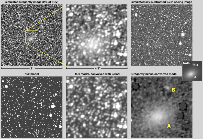
2.2 Illustration using artificial data

We illustrate the method with artificial data. An image of $21\farcm 3\times 21\farcm 3$ is created, containing $10^{4}$ stars, $5\times 10^{4}$ galaxies, and a constant sky background. The magnitude distributions follow power laws, with slopes $0.6$ for the stars (appropriate for an isotropic distribution) and $0.45$ for the galaxies (e.g., Lilly, Cowie, & Gardner 1991). The distribution of half-light radii of the galaxies is uniform between 0 and $2\farcs 5$; 40 % follow $r^{1/4}$ (de Vaucouleurs) profiles and 60 % follow exponential profiles. Two low surface brightness galaxies are added to the image. Their structure and surface brightness profiles are modeled on that of the UDG Dragonfly 44 ($R_{\rm e}=4.7$ kpc, $\mu_{0,V}=24.1$ mag arcsec^-2, and Sersic index $n=0.94$; van Dokkum et al. 2017), with one of the galaxies placed at 20 Mpc (galaxy A) and the other at 100 Mpc (galaxy B).

The image is generated at two resolutions and pixel sizes. The high resolution image has a pixel size of $0\farcs 25$ and a PSF that follows a Moffat profile with $\beta=2.5$ and FWHM = $0\farcs 75$, typical for wide field survey data of telescopes such as CFHT and Subaru. The low resolution image is tailored to Dragonfly, with a pixel size of $2\farcs 5$ and FWHM = $5\farcs 9$. The PSF is given an ellipticity of $\epsilon=0.2$ (and a position angle of 30^°) to simulate guiding or focus errors. To simulate realistic sky subtraction artifacts in the high resolution image we modeled and subtracted its sky using the default SExtractor settings, with a mesh size of $64\times 64$ pixels.

The low resolution image is shown in the top left panel of Fig. 1, with a zoom of the area containing the low surface brightness galaxies in the top middle panel. The images of these galaxies are highly contaminated by stars and galaxies. Galaxy A is visible but it is difficult to discern its structure and size. Galaxy B cannot be identified reliably in these data, as its appearance is similar to many other structures (blended faint stars and galaxies) in the image. We quantified this by calculating the number of pixels that are brighter than $\Sigma_{10}$, the mean galaxy surface brightness within $10\times 10$ pix². Nine percent of all pixels in the image are brighter than $\Sigma_{10}$ of galaxy A, and 36 % are brighter than $\Sigma_{10}$ of B.

The sky-subtracted high resolution image is shown at top right. Light from stars and compact galaxies cover a much smaller fraction of the pixels owing to the $10\times$ narrower PSF. Galaxy B is now just-visible as a low surface brightness patch in the top part of the frame. Galaxy A is also visible but is fainter and smaller than it should be due to the sky subtraction. Also, the contrast between both galaxies and the background is low, and they could easily be mistaken for ghosts, flat fielding errors, or other issues in the data reduction.

The bottom panels show the multi-resolution filtering process applied to these data. We performed the analysis with the mrf code, which is described in detail in the next Section. First a flux model is created by multiplying the high resolution image by an object mask created with SExtractor (bottom left panel in Fig. 1). Next, the flux model is convolved with a kernel to match the low resolution image (bottom middle panel). The convolved model looks very similar to the low resolution image shown above it, except that it does not include the low surface brightness objects. The final step is the subtraction of this convolved model from the low resolution image. The two low surface brightness objects are prominent in the residual image, shown in the bottom right panel. The total fluxes of objects A and B are recovered to $\approx 95$ % and $\approx 80$ % respectively.

Figure 2: Top left: Small section ($6\farcm 5\times 7\farcm 3$) of the 10 deg² Dragonfly $r$-band image of M101, centered on the satellite galaxy M101-DF3 (Merritt, van Dokkum, & Abraham 2014; Danieli et al. 2017). This image is referred to as $I^{\rm L}$ in the text. Top middle: The same area as observed with CFHT in the context of the CFHT Lensing Survey ($I^{\rm H}$). The resolution is far superior to that of Dragonfly, but M101-DF3 is fainter due to sky subtraction errors on large scales. There is faint large scale PSF structure around the bright star at the top of the frame. Top right: Initial flux model $F^{\rm H(3)}$, generated by multiplying a SExtractor object mask by $I^{\rm H(3)}$. This model contains all compact sources in the field and also some low surface brightness emission from M101-DF3. Bottom row: Zoomed views of M101-DF3 ($2\farcm 1\times 2\farcm 1$).

3 Implementation

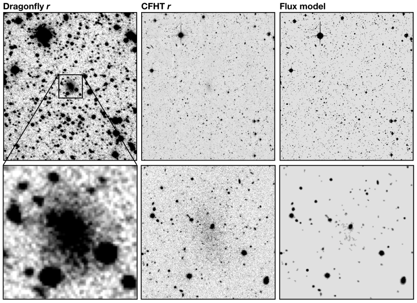
The method is implemented in the python package mrf. The individual steps are demonstrated using Dragonfly imaging of a low surface brightness satellite of the nearby face-on spiral galaxy M101. M101 is at a distance of 7 Mpc (Lee & Jang 2012), and it is one of the nearest massive galaxies. It was observed in May and June 2013 in the SDSS $g$ and $r$ filters with an eight-lens configuration. The pixel size of the reduced images is $2\farcs 0$, and the FWHM image quality is $\approx 6\farcs 7$. The image is publicly available. In van Dokkum, Abraham, & Merritt (2014) and Merritt et al. (2016a) we measured the light profile of the galaxy, constraining the mass of its stellar halo. In Merritt et al. (2014) we presented seven previously-uncataloged low surface brightness objects in the M101 field. In follow-up studies with the Hubble Space Telescope (HST) we found that four of these seven objects are intrinsically-large background galaxies (Merritt et al. 2016b) and three are satellites of M101 (Danieli et al. 2017). Here we focus on a small region centered on one of these confirmed satellites, M101-DF3 (see Fig. 2). The galaxy has an effective surface brightness of $\mu_{e,g}=27.4\pm 0.2$ and an effective radius $r_{e}=30\arcsec\pm 3\arcsec$ (Merritt et al. 2014). Its distance, as measured from the tip of the red giant branch, is $D=6.5\pm 0.3$ Mpc (Danieli et al. 2017).

3.1 High resolution M101 images

The M101 field has publicly available imaging from the Canada France Hawaii Telescope (CFHT), obtained in the context of the CFHT Lensing Survey (Heymans et al. 2012). The exposure times in $g$ and $r$ were 2500 s per filter. The CFHT images of M101-DF3 are shown in the middle panels of Fig. 2.

The CFHT and Dragonfly data are brought to a common reference frame. This frame has a finer pixel scale than the Dragonfly data, so that the subpixel flux distribution of compact objects is properly modeled. The low resolution Dragonfly image $I^{\rm L}$ is sampled onto a grid with $1/3$ the pixel size ($0\farcs 67$ in the case of M101) using a third order polynomial for the interpolation. This subsampled image is denoted $I^{\rm L(3)}$ and its size is $3n\times 3m$ if the size of $I^{\rm L}$ is $n\times m$. For each filter the CFHT image $I^{\rm H}$ is projected onto the $I^{\rm L(3)}$ frame using the WCS information from the headers of both images and a third order polynomial for interpolation. Prior to transforming $I^{\rm H}$ to $I^{\rm H(3)}$ the image was binned $2\times 2$ and convolved with a $\sigma=1$ pixel Gaussian, as this mitigates projection errors going from the $0\farcs 186$ CFHT pixel scale to that of $I^{\rm L(3)}$. In general, care should be taken that the pixel size of the subsampled low resolution data is within a factor of a few of the resolution of the high resolution data.

Next, the filter systems are matched. For both Dragonfly and CFHT data are available in the $g$ and $r$ filters. However, even though the Dragonfly filter curves are nearly identical to those used in SDSS and many other surveys, the total system response is not. The SBIG STF-8300 cameras have a low quantum efficiency in the blue, which means that the effective Dragonfly $g$ is slightly redder than SDSS $g$. It is therefore necessary to bring the CFHT images onto the same filter system as the Dragonfly data.

The mrf code can interpolate between high resolution images in two filters. It is assumed that

$$I^{L(3)}(g_{\rm DF})\propto I^{H(3)}(g_{\rm CFHT})\left(\frac{I^{H(3)}(g_{\rm CFHT})}{I^{H(3)}(r_{\rm CFHT})}\right)^{\alpha_{g}},$$ (5)

with an equivalent expression for the $r_{\rm DF}$ band. The value of $\alpha$ is determined from synthetic photometry of stars in the Gunn & Stryker (1983) atlas; we find $\alpha_{g}\approx+0.05$ and $\alpha_{r}\approx+0.01$.

The ratio $I^{\rm H(3)}(g_{\rm CFHT})/I^{\rm H(3)}(r_{\rm CFHT})$ is only well-determined in regions with a high S/N ratio in both filters, and a direct application of Eq. 5 to the high resolution images would lead to an extremely noisy interpolated image. We therefore create a color correction image $C$ such that $I^{\rm H(3)}(g_{\rm DF})=I^{\rm H(3)}(g_{\rm CFHT})\times C^{\alpha}$. The correction image is based on the SExtractor segmentation map (see below), with all pixels belonging to an object set to the ratio of the SExtractor catalog fluxes in $g_{\rm CFHT}$ and $r_{\rm CFHT}$. As the catalog fluxes are much better determined than the flux in an individual pixel this interpolation method is more robust than a direct division. We caution that this procedure works best if the effective wavelengths of the high resolution and low resolution data are reasonably close.

3.2 Construction of the high resolution flux model

Objects are identified in $I^{\rm H(3)}$ using sep (Barbary 2016), which is a Python version of SExtractor. The SExtractor parameters can be adjusted for the particular dataset that is being analyzed; as the aim is to detect compact sources the code is typically run with a low minimum number of connected pixels (2 in this example), a low threshold for deblending ($5\times 10^{-4}$), and a fairly fine grid for the background model ($64\times 64$ pixels). The code produces a catalog of objects with positions and fluxes, as well as a segmentation map $S^{\rm H(3)}$. The value of each pixel in $S^{\rm H(3)}$ is that of the ID of the object that the pixel is a part of. We create an object mask from $S^{\rm H(3)}$:

$$M^{\rm H(3)}=\begin{cases}0,&\text{if}\ S^{\rm H(3)}=0\\ 1,&\text{otherwise.}\end{cases}$$ (6)

Next, objects that should not be subtracted from the Dragonfly image are removed from the mask. An example where this might be the case is a study of the stellar halos or tidal features around a set of galaxies in the image; it is then desirable to retain the high surface brightness regions of these galaxies in the Dragonfly data. The mrf code can be supplied with objects that need to be retained, as specified by their RA, DEC positions. For each object the ID is found in $S^{\rm H(3)}$ from the value of the pixel that is closest to this position. All pixels that have this same value in $S^{\rm H(3)}$ are identified, and set to zero in $M^{\rm H(3)}$. Note that bright stars and low surface brightness objects are also removed from the model, at a later stage (see § 3.4, 3.5, and 3.7).

The high resolution flux model is then created by multiplying the image by the object mask:

$$F^{\rm H(3)}=I^{\rm H(3)}\times M^{\rm H(3)}.$$ (7)

This initial flux model is shown in the rightmost panels of Fig. 2, for the $r$ band. The model contains stars, high surface brightness galaxies, and (parts of) low surface brightness galaxies and features. It may contain artifacts such as diffraction spikes, to the extent that SExtractor identifies them as objects. It does not include any emission outside of the segmentation map, that is, it ignores object flux beyond the scaled Kron radius (see Bertin & Arnouts 1996). To account for this the mask can optionally be expanded by convolving it with a circular broadening function, prior to creating $F^{\rm H(3)}$. This was not done in this example.

Figure 3: Creation of the convolution kernel $K$ for the M101 image that is used as a demonstration of the implementation. Top row: Bright, non-saturated, compact objects in the high resolution CFHT image. Most of the 20 objects are stars. The third and fourth example objects were chosen to illustrate that the few compact galaxies produce very similar kernels as stars, as expected. Middle row: Dragonfly images of the same objects. Bottom row: Convolution kernels to go from the top row to the middle row, derived by an inverse Fourier transform of the quotient of the Fourier transforms of the two images. The convolution kernel that is used in the analysis is the median of these twenty individual kernels. Each panel is $29\arcsec\times 29\arcsec$, sampled at $0\farcs 67$ pix^-1 (1/3 of the pixel scale of the Dragonfly M101 data).

3.3 Convolution kernel

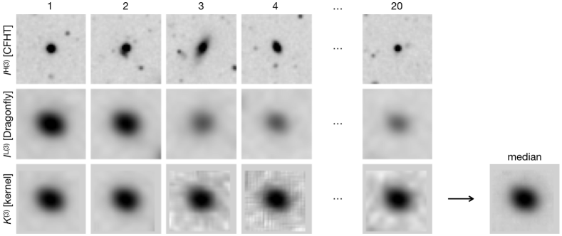
The convolution kernel to bring the high resolution model to the Dragonfly resolution is created using the Fourier quotient method, as explained in § 2.1. The actual kernel that is used is the median of a large number (typically 20–30) of individual kernels. These are created from image segments that are centered on bright, unsaturated objects and are spread evenly over the image.

In practice the following steps are taken. First, all objects in the $I^{\rm H(3)}$ catalog that are close to the edge of the image or have a flux greater than a user-defined value are discarded. This step serves to remove bright objects that are saturated in either $I^{\rm H(3)}$ or $I^{\rm L(3)}$ or for other reasons should not be taken into account. Typical values are $0.01<f_{\rm max}<0.1$, with $f_{\rm max}$ the user-defined brightness with respect to the fifth-brightest object in the catalog. The optimal value depends on the depth of the images, the seeing, the number of very bright stars in the field, and the minimum S/N ratio that is required: the parameter $f_{\rm max}$ effectively controls from which part of the luminosity function the kernel objects are drawn. An appropriate choice of $f_{\text{max}}$ is critical for obtaining a clean residual map $R$.

The next-brightest $N_{\rm kernel}$ objects in the catalog are selected, with $N_{\rm kernel}$ a user-defined parameter. Several of these objects will be large galaxies or close to other bright stars or galaxies, making them less suitable as inputs to the median kernel. We remove such objects by requiring that $b/a>0.6$ and $0.8<I^{\rm H}_{i,\rm section}/I^{\rm H}_{i,\rm catalog}<1.5$, that is, that they are fairly round and that the flux in the image section that is used for the Fourier transforms is close to the catalog flux. For the remaining objects (nearly all of them isolated stars) we determine the median kernel using Eqs. 3 and 4. We note that the individual kernels, and the median kernel, are not normalized to unity. Instead, the integrated flux is equal to the flux ratio (in ADU) between the high resolution and low resolution images. The kernel therefore implicitly accounts for any relative errors in the zeropoints of the two images. The process is illustrated in Fig. 3 for the M101 example. In this example, 17 of the 20 compact objects are stars; as shown in columns 3 and 4 of Fig. 3 the few compact galaxies that satisfy the criteria produce identical kernels as stars (as expected from the Fourier quotient method).

Figure 4: Top left: Flux model $F^{\rm H(3)}$ after removing bright stars and low surface brightness emission on the scale of the Dragonfly PSF. Top middle: Flux model convolved with kernel $F^{\rm L}$, resampled to the Dragonfly pixel scale. Top right: Residual image $I^{\rm L}-F^{\rm L}$. Most compact sources are removed from the Dragonfly data, while bright stars and low surface brightness emission are preserved. The bright stars are treated separately. Bottom row: zoomed views.

3.4 Removal of low surface brightness emission from the model

Prior to convolving the flux model with the kernel two classes of sources are removed from it: bright stars (see § 3.5) and objects that have the spatial scale of the Dragonfly PSF and are fainter than a particular surface brightness threshold. This step serves to ensure that only compact objects are subtracted from the Dragonfly data. Without it, object catalogs created from filtered Dragonfly data would be difficult to interpret as any low surface brightness objects that were entirely or partially detected in the high resolution images would no longer be present in the images. The M101-DF3 example is a good illustration: as can be seen in the bottom right panel of Fig. 2 small sections of the galaxy are in the initial flux model, as they are identified as a clump of low surface brightness objects with SExtractor.

We remove low surface brightness objects in the following way. An image is created that is sensitive to the spatial extent of objects with respect to the Dragonfly PSF:

$$E=\frac{F^{\rm H(3)}}{F^{\rm H(3)}\ast K}.$$ (8)

If $\langle E\rangle\sim 1$, with the angled brackets indicating the average over all pixels belonging to the object according to the segmentation map, its spatial extent is larger than the Dragonfly PSF. If $\langle E\rangle\gg 1$ it is a compact object that should be retained in the model and subtracted from the Dragonfly data.

Objects are removed from the model (and hence retained in the Dragonfly data) if they satisfy the following two criteria: $\langle E\rangle<E_{\rm lim}$, with $E_{\rm lim}$ a user-defined value that is set to $E_{\rm lim}=6$ for the M101 data; and $\langle F^{\rm H(3)}\rangle<F_{\rm lim}$, with $F_{\rm lim}$ a maximum surface brightness. In the case of the M101 example this limit was set to the equivalent of a surface brightness of $\mu_{r}=24.0$ mag arcsec^-2. The results are very similar when changing these limits by factors of $\sim 2$. Optionally a minimum object area can be specified as an additional criterion.

Figure 5: Top left: Model for the bright stars that were removed from the flux model. Top middle: Residual image after subtracting the bright stars. Top right: Residual image after masking the regions corresponding to the brightest pixels in the convolved flux model, as well as stars with $m_{r}<12.5$ (only one in the region that is shown). The bar at the bottom indicates the conversion of grey level to $r$-band surface brightness, in units of mag arcsec^-2. Bottom row: zoomed views.

3.5 Removal of bright stars from the model

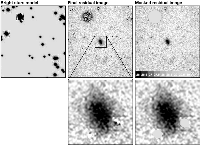
The MRF procedure is very effective in removing faint compact sources but it is not suitable for the removal of very bright stars. There are two reasons for this. First, the kernel is only $36\arcsec\times 36\arcsec$, and this is smaller than the extent of the wings of bright stars. Creating larger kernels is possible (the kernel size is a user-defined parameter in the mrf code) but the S/N ratio in the outer parts is low for the unsaturated stars and galaxies that are used to create it. The second issue is saturation, particularly in the high resolution data. Typical high resolution images (including the CFHT data used in the example) are relatively long exposures on large telescopes, and many of the brighter stars and galaxies are satured in their centers. This leads to several distinct problems. The first is bleeding in the high resolution data, as is happening for the bright star in the upper left of the example image in Fig. 2. These erroneous features make their way into the residual image as strongly negative pixels as they are part of the flux model. The second is that the flux of these objects in the high resolution data is lower than the true brightness, sometimes severely so. As a result, bright stars in the flux model are too faint, leaving positive residuals in the final star-subtracted image. The third is centroiding errors, which cause strong positive and negative residuals.

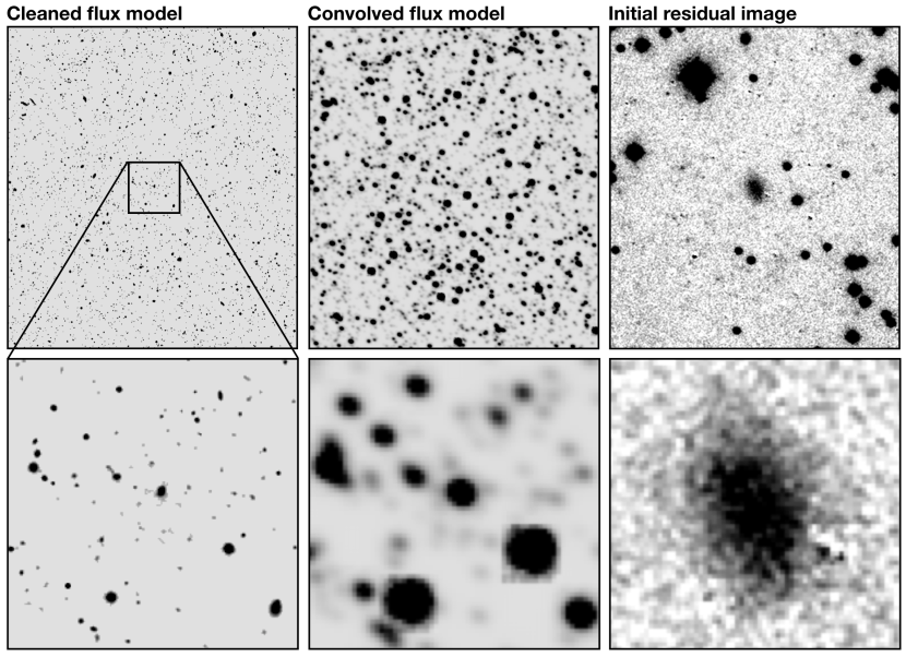
For these reasons the mrf code removes the brightest objects from the flux model, down to a user-defined magnitude. The code outputs a list of the objects (mostly stars) that are excluded from the model. At a later stage they are identified in, and removed from, the Dragonfly image (§ 3.7). In the M101-DF3 example the magnitude limit that is used is $m_{r}<17.5$. The “cleaned” flux model, with low surface brightness emission and bright stars removed, is shown in the left panels of Fig. 4.

3.6 Convolution of the model and subtraction

The cleaned flux model is convolved with the median kernel to match the Dragonfly resolution,

$$F^{\rm L(3)}=F^{\rm H(3)}\ast K,$$ (9)

and subtracted:

$$R^{\rm(3)}=I^{\rm L(3)}-F^{\rm L(3)}.$$ (10)

The residual is then binned to the original grid of the Dragonfly data to create $R$. The convolved model $F^{\rm L}$ (rebinned to the Dragonfly resolution) is shown in the middle panels of Fig. 4. The residual $R$ is shown in the right panels. The residual image consists of low surface brightness emission, the bright stars that were purposely left in the image, and artifacts due to imperfect modeling of the centers of subtracted stars.

3.7 Subtraction of bright stars from the residual image

Bright stars are modeled and subtracted in a way that is analogous to that described in van Dokkum et al. (2014), Merritt et al. (2014), and Merritt et al. (2016a). First, a catalog of objects in the residual image is created with SExtractor. Next, the catalog is cross-matched with the objects that were removed from the flux model, and only those that are matched are retained. This matching requirement ensures that no spurious bright objects in the high resolution image are subtracted from the Dragonfly data, and that objects that were already subtracted as part of the convolved flux model are not subracted twice. A model PSF is created by taking the median of image cutouts of the matched stars, after shifting them to the same sub-pixel position and normalizing them. The normalization is not done by the total (or AUTO) flux but by the flux in an annulus between $r=3$ pix ($6\arcsec$) and $r=6$ pix ($12\arcsec$), to avoid any saturated pixels. In Dragonfly images even very bright stars are typically not saturated beyond $r=6\arcsec$, due to the steep fall-off of the PSF (see Abraham & van Dokkum 2014).

For each bright object the model PSF is scaled to its total flux (taking saturation into account) and placed at its location, with sub-pixel accuracy. The size of the model PSF is a user-defined parameter; in this example we use $48\times 48$ pixels, or $96\arcsec\times 96\arcsec$. The image containing the scaled models is shown in the top left panel of Fig. 5. This image is subtracted to create the final residual image $R$, shown in the middle panels of Fig. 5.

Although the subtraction is adequate for this M101 region, some Dragonfly data include individual very bright stars whose light at large radii cannot be modeled with this procedure. The mrf code includes the option to extend the stacked 2D model PSF to radii $>30\arcsec$ (commonly referred to as the aureole; see King 1971) using an analytic function. As discussed in Q. Liu et al., in preparation, the form of the aureole function is a composite of powerlaws:

$$I_{\rm au}(R)=\sum_{i=0}^{k}{\frac{A_{i}}{R_{i}^{-n_{i}}}R^{-n_{i}}},$$ (11)

with $k=2$. The constants $A_{i}$ are not fit parameters but fully determined by the values of $R_{i}$, $n_{i}$, and the total magnitude of the star. The transition radii $R_{i}$ and powerlaw slopes $n_{i}$ are adjustable in the code as they depend on the atmospheric conditions at the time of the observation. In § 4.3 we show an example of a previously-published image with several bright stars, where the analytic function improves the subtraction. In the M101 image discussed here the analytic function extension was not used.

Figure 6: A possible very faint nucleated dwarf galaxy in the model-subtracted M101-DF3 image. The galaxy has an absolute magnitude of $M_{r}\approx-8.0$ if it is at the distance of M101. Note that the very bright and large object in the top panel is M101-DF3 itself, which was unknown prior to 2014 and discovered in these Dragonfly data (Merritt et al. 2014).

3.8 Masking of artifacts in the final residual image

The final residual image is not free of artifacts but their locations can be robustly predicted. They mostly occur in locations were bright stars were subtracted, as even a small error in the flux model can produce a large residual in regions where the counts are high. All regions in the residual image are masked where the subtracted model $F^{\rm L}>F_{\rm lim}$, with $F_{\rm lim}$ a user-defined parameter. Only the model flux is used to determine whether to mask pixels in the residual image, and not the residual itself; this is to prevent the masking of relatively bright objects that may be present after the subtraction of the model. The mask can optionally be extended to include pixels neighboring those that are brighter than $F_{\rm lim}$.

The very brightest stars are also masked, using a circular mask with a user-defined radius for objects down to a user-defined magnitude. For the M101-DF3 example we use a limit of $m_{r}<12.5$ and a radius of 40 pixels ($80\arcsec$). Only one object, the $m_{V}=10.9$ star TYC 3852-845-1, falls in this category. The masked residual image of M101-DF3 is shown in the right panels of Fig. 5. We note that the required masking impacts far less pixels than would be the case if the convolved flux model had not been subtracted. In the M101-DF3 example, a simple mask applied to the original Dragonfly image would cover $\sim 20\times$ more pixels than the mask shown in Fig. 5. For a visual impression, compare the left panels of Fig. 2 to the right panels of Fig. 4.

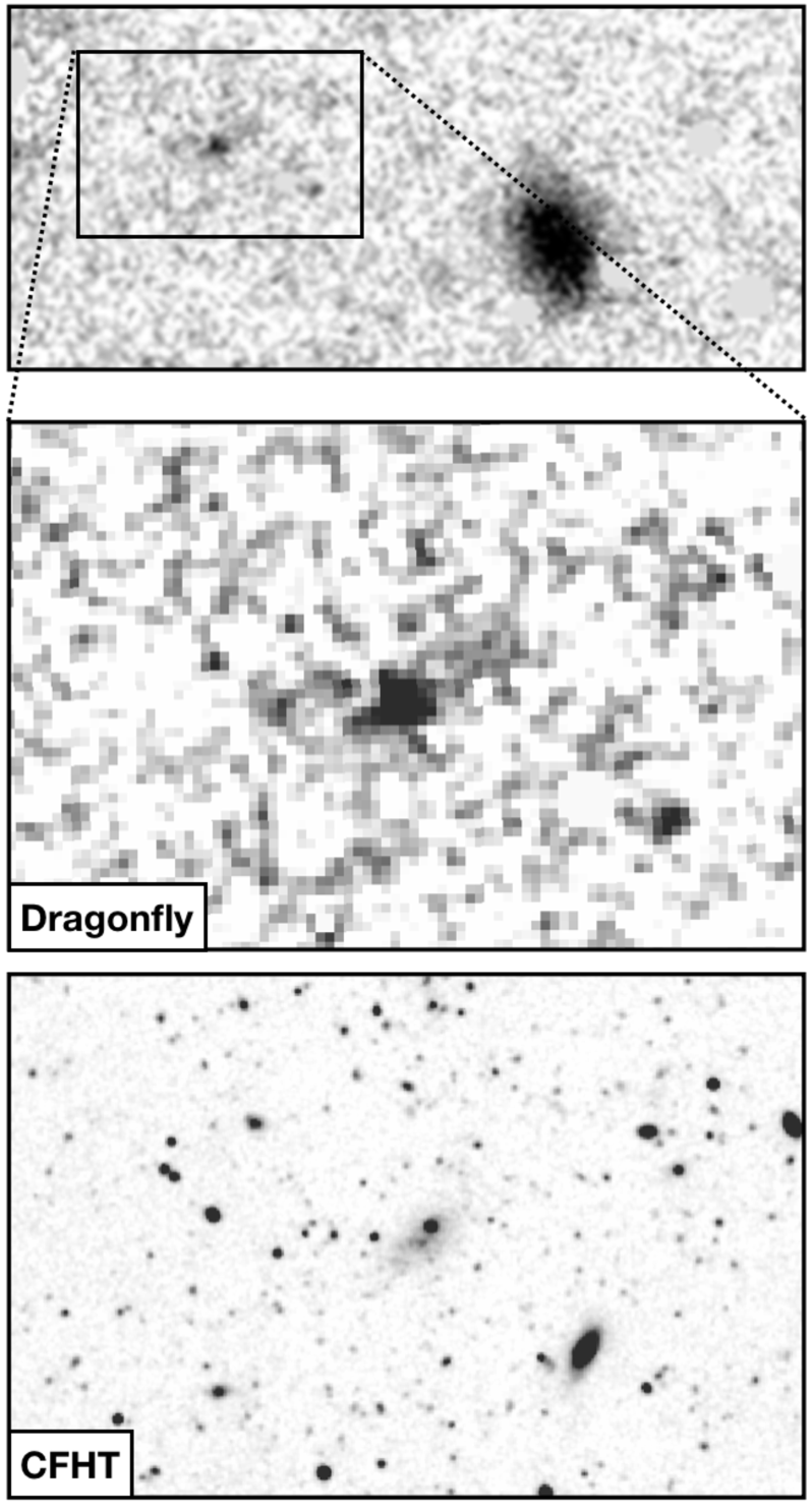
The final masked image shows M101-DF3 itself very clearly. In addition, several other faint sources are still present after subtraction of the convolved flux model and masking. These fall in several categories: compact variable sources, such as variable stars and active galactic nuclei; low surface brightness emission associated with galaxies, such as tidal tails and stellar halos; and low surface brightness dwarf galaxies. One of the brightest examples is shown in Fig. 6. This low surface brightness object is a possible nucleated dwarf galaxy, at ${\rm RA}=14^{\rm h}3^{\rm m}27\fs 38$, ${\rm DEC}=53\arcdeg{}37\arcmin{}51\farcs 8$ (J2000). It is not in the sample of faint low surface brightness objects of Carlsten et al. (2019), and given its proximity to M101 it is unlikely that it is a member of the background NGC 5485 group (see Merritt et al. 2016b, Karachentsev & Makarova 2019). Its $r$-band magnitude in the Dragonfly data is $m_{r}\approx 21.2$. If it is at the distance of M101 its absolute magnitude is $M_{r}\approx-8.0$, which would place it among the lowest luminosity dwarf galaxies yet identified outside of the Local Group (see, e.g., Smercina et al. 2017, Mihos et al. 2018).

Figure 7: Top panels: Dragonfly $r$-band image of M51, with two different scalings. The displayed image is a $42\arcmin\times 38\arcmin$ cutout. Bottom left: After multi-resolution filtering. Bottom right: Median filtered version of the multi-resolution filtered image. Two $\mu_{B}\sim 29$ mag arcsec^-2 features that were discovered by Watkins, Mihos, & Harding (2015) are indicated.

Figure 8: Left: Small ($12\farcm 4\times 22\farcm 9$) section of the Dragonfly $g+r$-band Coma image that was used in van Dokkum et al. (2015) to identify 47 ultra-diffuse galaxies (UDGs) in the cluster. This section contains two UDGs, Dragonfly 44 and DFX1. Right: The same region after multi-resolution filtering, using 300 s CFHT images to construct the flux model. The two UDGs are now the brightest objects in the image. The insets show their HST images, with extended sources masked (see van Dokkum et al. 2017).

Figure 9: Top: The stellar stream system of NGC 5907, as imaged by Martínez-Delgado et al. (2008). Middle: Dragonfly $g+r$ image of the same region, after subtracting compact emission. The mrf code was run with aureole modeling. Bottom: The same as the middle image but with areas masked where the flux model exceeds a certain threshold. Thanks to the aureole modeling this image shows less residuals around bright stars than that presented in van Dokkum et al. (2019).

4 Other Examples

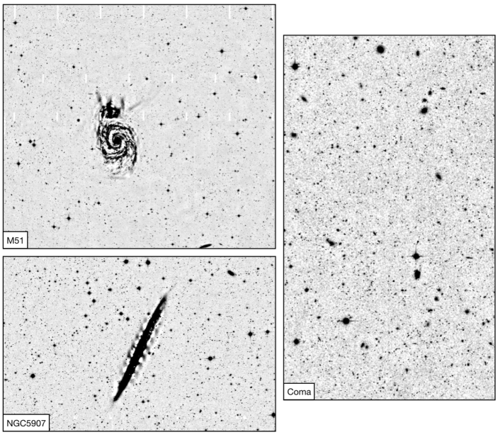
Here we apply the MRF technique to three additional Dragonfly datasets, to demonstrate the method in other contexts. The high resolution images of the three objects that are used in the analysis are shown in Fig. 10 in Appendix B. Other applications of the MRF technique on Dragonfly observations of nearby galaxies may be found in van Dokkum et al.  (2019), Gilhuly et al. (2019), and J. Li et al., in preparation.

4.1 M51

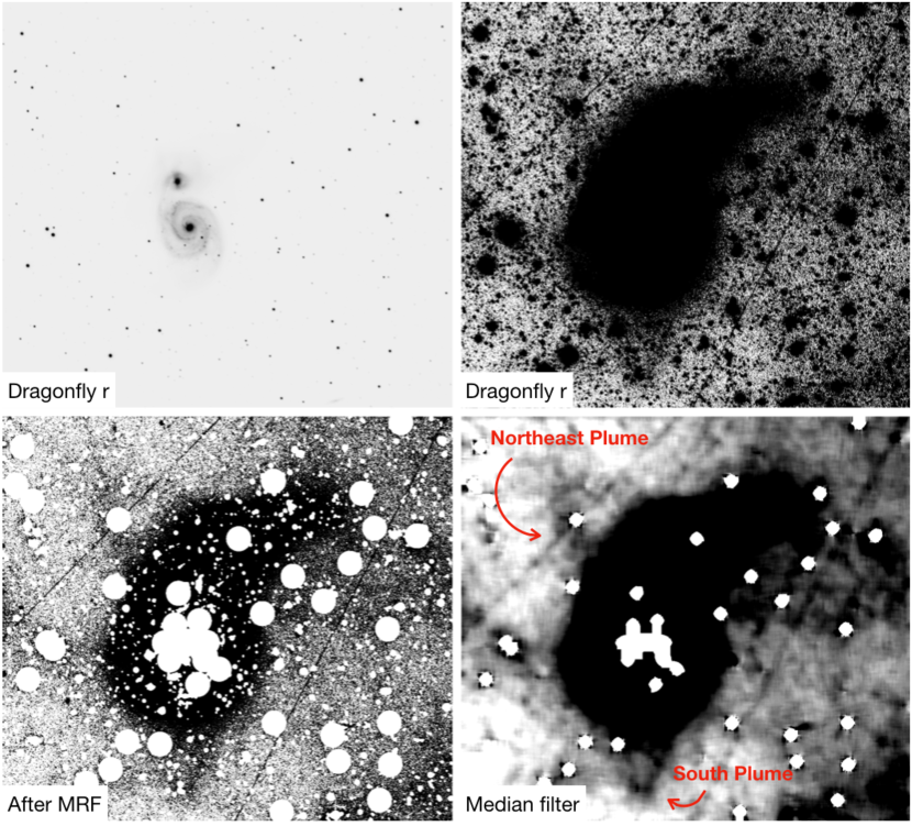
The interacting galaxy pair NGC 5194 and NGC 5195 (M51) was our first-light target with the upgraded 48-lens Dragonfly telescope and was observed on July 3 2016. Not all the lenses were operational all the time. The equivalent exposure time for a 100 % operational array with 24 lenses in each filter is 6950 s in $g$ and 6000 s in $r$. A section of the $r$-band image, centered on M51, is shown in the top panels of Fig. 7, with two different scalings. The reduction was performed with an early version of our pipeline and did not remove satellite trails.

The pair is embedded in an extensive tidal debris field. Despite many years of observations of this system, Watkins et al. (2015) discovered two previously-unknown tidal features in extremely deep images obtained with the Burrell-Schmidt telescope on Kitt Peak: the “South Plume” and the “Northeast Plume”, with surface brightness $\mu_{B}\sim 29$ mag arcsec^-2 (see Watkins et al. 2015). Here we determine whether these features can be seen in the Dragonfly data as well, after applying the MRF technique.

The mrf code is run with very similar parameters as in the M101-DF3 example. The high resolution data is again from CFHT: M51 was observed for 525 s in the $r$-band with Megacam on April 4 2007. We obtained the reduced image from the CFHT Archive. The results are shown in the bottom left panel of Fig. 7. After removal of the compact sources tidal features are more easily detected. This is illustrated in the bottom right panel, which shows the MRF image after applying a $21\times 21$ pixel ($52\farcs 5\times 52\farcs 5$) median filter. The two plumes discovered by Watkins et al. (2015) are readily seen in the Dragonfly image (see also Rich et al. 2019).

4.2 Ultra-diffuse galaxies in the Coma cluster

In 2015 a large population of faint, intrinsically-large galaxies was identified in the Coma cluster with the Dragonfly telescope (van Dokkum et al. 2015). These objects have sizes that are close to the Dragonfly PSF ($\sim 5\arcsec$) and it was difficult to isolate them against a background of many thousands of other objects. Later studies used wide-field imaging data from conventional telescopes with much better seeing to find UDGs in clusters and the general field, with great success (see, e.g., Koda et al. 2015; van der Burg et al. 2017; Román & Trujillo 2017; Danieli & van Dokkum 2019). Here we return to the original Dragonfly Coma data, to determine whether the MRF technique is able to efficiently identify these objects.

We use CFHT $g$ and $i$ images for creating the flux model. These data are described in van Dokkum et al. (2015) and Danieli & van Dokkum (2019). Neither of these filters is a good match to the Dragonfly ones, and instead we derive a color term to go from CFHT $g$ and $i$ to the sum of the Dragonfly $g+r$ images. Nevertheless, we find that the quality of the image subtraction is limited by the mismatch between the filters.

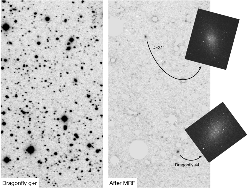
The Dragonfly $g+r$ image is shown in the left panel of Fig. 8. We focus on a $12\farcm 4\times 22\farcm 9$ section that contains two UDGs, Dragonfly 44 and DFX1 (see van Dokkum et al. 2017). The galaxies are not easily distinguished from other sources in the field, which is why van Dokkum et al. (2015) used a complex multi-stage process to eliminate faint objects from an initial candidate list of 6624. The right panel shows the same region after applying the mrf code, with default parameters. The two UDGs are now the two brightest objects in this region, and they can readily be identified using standard image detection software.

4.3 The tidal stream of NGC 5907

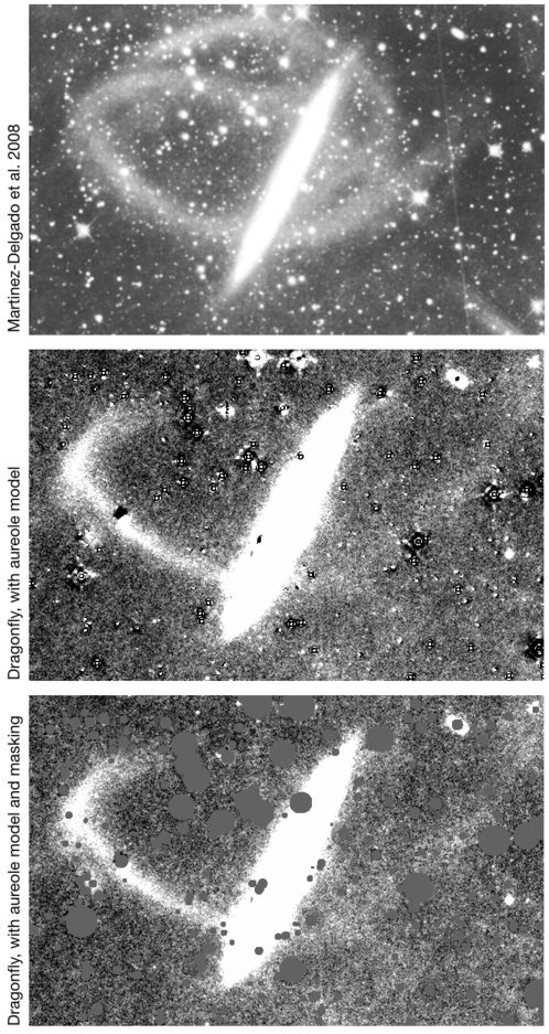
In a previous paper (van Dokkum et al. 2019) we applied the mrf methodology to a deep Dragonfly image of the edge-on galaxy NGC 5907. The galaxy has a curved tidal stream, discovered by Shang et al. (1998). Martínez-Delgado et al. (2008) found that the stream consists not of one but of two loops, wrapping twice around the galaxy. However, the Dragonfly data, as well as recent observations by Muller et al. (2020), failed to confirm this second loop.

There are several bright stars in the NGC 5907 field, and some of these are close to the purported second loop (see van Dokkum et al. 2019). In our published mrf analysis no attempt was made to subtract the extended aureoles of these stars. Since then we implemented the optional analytic PSF extension of Eq. 11, and here we show the improved subtraction that results from this. We use transition radii of $R_{0}=5\arcsec$, $R_{1}=71\arcsec$, and $R_{2}=151\arcsec$, and powerlaw indices of $n_{0}=3.24$, $n_{1}=2.53$, and $n_{2}=1.22$. These values are determined from a group of very bright stars in the wider Dragonfly field, $\approx 45\arcmin$ to the Southwest of NGC 5907 itself (see Fig. 1 of van Dokkum et al. 2019). The powerlaw model is tied to the empirical stacked 2D PSF at $R=30\arcsec$, and truncated at $R=20\arcmin$ to ensure that the integrated model flux is finite.

The results are shown in Fig. 9. Here we focus on the small region of the Dragonfly image that overlaps with the image of Martínez-Delgado et al. (2008); for a complete analysis we refer the reader to van Dokkum et al. (2019). The aureole modeling improves the subtraction of bright stars compared to the version of the code that was used in our previous analysis.

5 Summary

We present a straightforward method to use high resolution data to remove compact sources of emission from low resolution data. The method reliably distinguishes blended compact sources from low surface brightness emission, something that is very difficult to achieve with standard techniques applied to low resolution images (see, e.g., van Dokkum et al. 2015). It is implemented in the mrf Python package, which we make publicly available. In Appendix A we discuss two variations of the technique: self-MRF, where a smoothed version of an image takes the place of the low resolution image $I^{\rm L}$, and cross-MRF, where two high resolution images are available from different telescopes and one is smoothed to create $I^{\rm L}$. Both are included in the public distribution of the mrf code.

The mrf tool is important for the correct interpretation of data from the Dragonfly Telephoto Array, as crowding is a significant problem for this telescope. By removing the confusing signal of blurred compact objects the benefits of Dragonfly, such as its wide field of view, low false positive rate, and its excellent control of scattered light, can be fully utilized. High resolution images of sufficient depth are generally readily available, as Dragonfly’s sensitivity to compact objects is equivalent to that of a 1 m telescope with $\approx 5\arcsec$ seeing. MRF has been applied to the analysis of data from the Dragonfly Edge-on Galaxy Survey (van Dokkum et al. 2019; Gilhuly et al. 2019), and is an integral part of the Dragonfly Wide Field Survey (Danieli et al. 2020), which aims to identify faint dwarf galaxies in a 400 degree² area. Looking ahead, images with a resolution of $\sim 0\farcs 2$ will be routinely available over large parts of the sky from EUCLID and/or WFIRST, and those data may serve as the high resolution flux model to aid searches for faint extended sources in deep images from large telescopes on the ground.

The present paper does not discuss systematic uncertainties which might be introduced by the technique. Filtered frames should be treated with caution: photometry at the location of removed objects is more uncertain than photometry in “pristine” regions, and incomplete removal of compact objects could lead to false positives in low surface brightness galaxy searches. How severe these issues are depends on the specific dataset and the specific science questions that are asked. We urge users of filtered data to incorporate the flux model and residual mask created by mrf in their object detection and photometry codes. In T. Miller et al., in preparation, we assess the recovery of total fluxes of realistic galaxy images injected in data from the Dragonfly Wide Field Survey. Performing photometry on the MRF-cleaned images yields total fluxes with no systematic bias and a random scatter of $0.08$ magnitudes.

Appendix A Variations: self-MRF and cross-MRF

The MRF code was developed to isolate low surface brightness emission by removing all compact sources from the image. The specific application, discussed extensively in the main text, is the “cleaning” of Dragonfly images using seeing-limited wide-field ground based data. However, in many cases no such intrinsically-low resolution imaging will be available, and most aspects of the MRF methodology for isolating low surface brightness emission can still be applied in those instances. In self-MRF, a smoothed version of an image is used as the low resolution model. This smoothed image takes the place of $I^{\rm L}$, and the code runs in the same way as in its standard implementation. The smoothing kernel can be tuned to the particular structures that the user intends to isolate; by experimenting on known dwarf galaxies in Hyper Suprime-Cam data we find that a convolution with an exponential kernel provides the best results. We note that self-MRF is essentially a variation of standard low pass filtering approaches (see, e.g., Greco et al. 2018b).

Another common situation is where two high resolution images are available, from different telescopes. Many extragalactic surveys cover overlapping sky areas, such as the GAMA fields (Driver et al. 2011). In cases where, for instance, data from Subaru and CFHT are available one data set can be smoothed to form $I^{\rm L}$ and the other can assume the role of $I^{\rm H}$. In this application, dubbed cross-MRF, the survey with the best low surface brightness sensitivity (typically, the one with the best sky subtraction) can be used for $I^{\rm L}$. An important advantage over self-MRF is that artifacts (such as diffraction spikes) are usually not present at the same location in two independent observations. Demonstrations of both self-MRF and cross-MRF are provided with the mrf GitHub distribution.

Appendix B High resolution images of the three examples

In Fig. 10 we show the public CFHT images of the three fields that are analyzed in § 4. These CFHT images are the high resolution data that are used to create the flux models. It is striking that no large scale low surface brightness emission is visible around M51 and NGC 5907. This is caused by the data reduction procedures that are applied to these publicly available CFHT data; as described in Gwyn (2008), the MegaPipe pipeline subtracts spatially-extended emission. For our purposes this oversubtraction is not an issue, but we note here that far superior results can be obtained from CFHT with Elixir-LSB, a low surface brightness-optimized reduction process (J. C. Cuillandre et al., in preparation).

Figure 10: The high resolution images that are used for the multi-resolution filtering of the Dragonfly images in Figs. 7, 8, and 9. Note the complementarity of these CFHT images and the Dragonfly images: the CFHT data have excellent point source sensitivity, but all spatially-extended low surface brightness emission was removed in the reduction process.