TUM-HEP-1235/19
NIKHEF/2019-048
CERN-TH-2019-176
October 28, 2019

Leading-logarithmic threshold resummation
of Higgs production in gluon fusion
at next-to-leading power

Martin Beneke,^a Mathias Garny,^a Sebastian Jaskiewicz,^a

Robert Szafron,^a,b Leonardo Vernazza,^c,d,e and Jian Wang^f
a Physik Department T31,
James-Franck-Straße 1, Technische Universität München,
D–85748 Garching, Germany
^b Theoretical Physics Department, CERN,
1211 Geneva 23, Switzerland
^c Institute for Theoretical Physics Amsterdam and
Delta Institute for Theoretical Physics,
University of Amsterdam, Science Park 904,
NL–1098 XH Amsterdam, The Netherlands
^d Nikhef, Science Park 105,
NL–1098 XG Amsterdam, The Netherlands
^eDipartimento di Fisica Teorica, Università di Torino,
and INFN, Sezione di Torino, Via P. Giuria 1, I-10125 Torino, Italy
^fSchool of Physics, Shandong University,
Jinan, Shandong 250100, China

We sum the leading logarithms $\alpha_{s}^{n}\ln^{2n-1}(1-z)$, $n=1,2,\ldots$ near the kinematic threshold $z=m_{H}^{2}/\hat{s}\to 1$ at next-to-leading power in the expansion in $(1-z)$ for Higgs production in gluon fusion. We highlight the new contributions compared to Drell-Yan production in quark-antiquark annihilation and show that the final result can be obtained to all orders by the substitution of the colour factor $C_{F}\to C_{A}$, confirming previous fixed-order results and conjectures. We also provide a numerical analysis of the next-to-leading power leading logarithms, which indicates that they are numerically relevant.

1 Introduction

The Higgs production cross section in gluon-gluon fusion is presently the most precisely computed observable in hadron-hadron collisions, as far as orders in perturbation theory (N³LO [1, 2, 3, 4] in the heavy-top approximation) and threshold resummation (N³LL [5, 6, 7, 8, 9, 10]) are concerned. In [11] we developed the framework for threshold resummation at next-to-leading power (NLP) using effective field theory, taking the first step beyond the leading-power resummation formalism in perturbative QCD [12, 13]. We applied it to the summation of the leading logarithms (LL) in the classic Drell-Yan process $q\bar{q}\to\gamma^{*}+X$. Given the interest in Higgs production both phenomenologically and for applying new methods to high-order calculations, we discuss the similarities and differences of NLP threshold resummation for Higgs production in gluon fusion compared to the case of a virtual photon in this paper. Although it is not the main focus of the work, we also provide a numerical analysis of the next-to-leading power leading logarithms, which indicates that they are numerically relevant.

The outline of this paper is as follows. In Sec. 2 we derive the factorization formula for single Higgs production at NLP in soft-collinear effective theory (SCET), identify the sources of NLP LLs, and derive the hard, soft, and collinear functions needed for resummation with LL accuracy. The resummation of NLP LLs via renormalization-group equations is contained in Sec. 3. In the same section we also expand the resummed result in $\alpha_{s}$, which provides both, a check of the resummed result by comparison with existing fixed-order expressions, and so far unknown logarithmic terms at higher order. Finally, in Sec. 4 we perform a numerical study of the NLP-resummed cross section.

For the sake of avoiding repetition, we build on [11] for basic definitions related to threshold resummation and SCET. We also recommend consulting that paper for the general logic of deriving the NLP factorization and simplifications at the leading-logarithmic order before continuing with this one.

2 Threshold factorization at NLP

We consider the process

$$A(p_{A})+B(p_{B})\to\mbox{H}(q)+X,$$ (2.1)

where $A(p_{A})$, $B(p_{B})$ represent the colliding protons, and $X$ denotes an unobserved QCD final state. The cross section for this process can be written as

$$\sigma=\frac{\alpha_{s}^{2}}{576\pi v^{2}}\sum_{a,b}\int_{0}^{1}dx_{a}\int_{0}^{1}dx_{b}\,f_{a/A}(x_{a})f_{b/B}(x_{b})\,\hat{\sigma}_{ab}(z),$$ (2.2)

where $f_{i/I}(x_{i})$ represent parton distribution functions and $v$ is the Higgs vacuum expectation value, $v^{2}=1/(\sqrt{2}G_{F})$. $G_{F}$ is the Fermi constant, and $\alpha_{s}$ without scale argument refers to the strong coupling at the $\overline{\rm MS}$ scale $\mu$. In the following, we consider only the gluon-gluon initial state and drop the indices $a,b$. Higgs production in gluon fusion occurs through a top loop, which couples the gluons to the Higgs boson. In the heavy-top-quark mass limit $m_{t}\gg m_{H}$, the Higgs boson couples to gluons via

$${\cal L}_{\rm eff}=C_{t}\left(m_{t},\,\mu\right)\,\frac{\alpha_{s}}{12\pi}\frac{H}{v}F^{A}_{\mu\nu}F^{\mu\nu A},$$ (2.3)

where

$$C_{t}\left(m_{t},\,\mu\right)=1+\frac{\alpha_{s}}{4\pi}(5C_{A}-3C_{F})+{\cal O}(\alpha_{s}^{2})\,.$$ (2.4)

The partonic cross section $\hat{\sigma}\equiv\hat{\sigma}_{gg}$ is a function of the dimensionless variable $z=m_{H}^{2}/\hat{s}$, where $\hat{s}=x_{a}x_{b}\,s$ represents the partonic centre-of-mass energy squared, and $x_{a}$, $x_{b}$ the momentum fractions of the gluons in the corresponding hadrons, defined through the parton momenta $p_{a}^{\mu}=x_{a}\sqrt{s}n_{-}^{\mu}/2$, $p_{b}^{\mu}=x_{b}\sqrt{s}n_{+}^{\mu}/2$. Our aim is to sum the leading logarithms in the series $\sum_{n=1}^{\infty}\sum_{m=0}^{2n-1}d_{nm}\ln^{m}(1-z)$ of next-to-leading power logarithms as was done for $q\bar{q}\to\gamma^{*}+X$ [11]. To this end, we start from the Higgs production cross section formula

$$\sigma=\frac{1}{2s}\int\frac{d^{3}\vec{q}}{(2\pi)^{3}2E_{q}}\sum_{X}|\langle HX|AB\rangle|^{2}(2\pi)^{4}\delta^{(4)}(p_{A}+p_{B}-q-p_{X}),$$ (2.5)

where the matrix element squared reads

$$\sum_{X}|\langle HX|AB\rangle|^{2} = \frac{\alpha_{s}^{2}(\mu)\,C^{2}_{t}(m_{t},\mu)}{144\pi^{2}v^{2}}$$ (2.6)

$$\times\,\sum_{X}\langle AB|\big{[}F^{A^{\prime}}_{\rho\sigma}F^{\rho\sigma A^{\prime}}\big{]}(0)|X\rangle\langle X|\big{[}F^{A}_{\mu\nu}F^{\mu\nu A}\big{]}(0)|AB\rangle.$$

The QCD operator $F^{A}_{\mu\nu}F^{\mu\nu A}$ is then matched to SCET operators. At leading power (LP) this involves the single operator

$$F^{A}_{\mu\nu}F^{\mu\nu A}(0)=\int dt\,d\bar{t}\,\widetilde{C}^{A0}(t,\bar{t}\,)\,J^{A0}(t,\bar{t}\,)\,,$$ (2.7)

where

$$J^{A0}(t,\bar{t}\,)=2g_{\mu\nu}\,n_{-}\partial{\cal A}^{\nu A}_{\,\bar{c}\perp}(\bar{t}n_{-})\,n_{+}\partial{\cal A}^{\mu A}_{\,c\perp}(tn_{+})\,,$$ (2.8)

$$C^{A0}(n_{+}p,n_{-}\bar{p}\,)=\int dt\,d\bar{t}\,e^{-i(n_{+}p)t-i(n_{-}\bar{p})\bar{t}}\,\widetilde{C}^{A0}(t,\bar{t}\,)\,.$$ (2.9)

Here $\mathcal{A}_{c\perp}^{\mu}$ denotes the collinear-gauge-invariant transverse collinear gluon field of SCET. The operator generates a collinear and an anti-collinear field and is non-local along the light-rays in the respective directions. The derivatives correspond to the large momentum components of the fields. With the normalization (2.8), the hard coefficient function is $\widetilde{C}^{A0}(t,\bar{t}\,)=\delta(t)\delta(\bar{t})+\mathcal{O}(\alpha_{s})$, or $C^{A0}(n_{+}p,n_{-}\bar{p})=1+\mathcal{O}(\alpha_{s})$ in momentum space. For LL resummation, the tree approximation will suffice.

Beyond LP the hard gluon-gluon-Higgs vertex is matched to higher-power SCET operators. The basis of such operators in the position-space SCET formalism is discussed in [19, 20, 21]. Following the same arguments as for $q\bar{q}\to\gamma^{*}$ [11, 26], to first subleading power in ($1-z$), i.e. to order $\lambda^{2}$, the LLs arise only from the time-ordered product of the LP operator $J^{A0}$ with the $\mathcal{O}(\lambda^{2})$ suppressed interactions from the SCET Lagrangian [27],

$$J_{A0,\,j}^{T2}(t,\bar{t}\,)=i\int d^{4}z\,{\bf T}\Big{[}J_{A0}(t,\bar{t}\,)\,{\cal L}^{(2)}_{j}(z)\Big{]},$$ (2.10)

where the index $j$ labels terms in the power-suppressed Lagrangian ${\cal L}^{(2)}(z)$. Thus, to obtain the NLP LL accurate amplitude, we simply add this operator to $J^{A0}(t,\bar{t}\,)$ in (2.7).

To proceed, one removes the soft-collinear interactions from the LP Lagrangian by a field redefinition [28], in which (anti-) collinear gluon fields are multiplied by adjoint soft Wilson lines ${\cal Y}_{+}$ (${\cal Y}_{-}$), defined as

$${\cal Y}^{AB}_{\pm}(x)={\bf P}\exp\bigg{\{}g_{s}\int_{-\infty}^{0}ds\,f^{ABC}\,n_{\mp}A^{C}_{s}(x+sn_{\mp})\bigg{\}}.$$ (2.11)

In terms of the decoupled collinear fields, which will be used below, the operator in (2.8) reads

$$J^{A0}(t,\bar{t}\,)=2g_{\mu\nu}\,{\cal Y}^{AC}_{-}(0)\,n_{-}\partial{\cal A}^{\nu C}_{\bar{c}\perp}(\bar{t}n_{-})\,{\cal Y}^{AD}_{+}(0)\,n_{+}\partial{\cal A}^{\mu D}_{c\perp}(tn_{+})\,.$$ (2.12)

The interaction Lagrangian is then also expressed in terms of the decoupled collinear field and the soft-gluon building block

$$\mathcal{B}_{\pm}^{\mu} = Y_{\pm}^{\dagger}\left[iD_{s}^{\mu}Y_{\pm}\right]\,,$$ (2.13)

evaluated at the appropriately multipole-expanded position, where $Y_{\pm}(x)$ represent soft Wilson lines in the fundamental colour representation:

$$Y_{\pm}(x)={\bf P}\exp\bigg{\{}ig_{s}\int_{-\infty}^{0}ds\,n_{\mp}A_{s}(x+sn_{\mp})\bigg{\}}.$$ (2.14)

An analysis of the interaction terms similar to [11], now for the Yang-Mills SCET Lagrangian, shows that only the two terms

$${\cal L}_{\rm 1YM}^{(2)} = -\frac{1}{2g_{s}^{2}}\,{\rm tr}\,\Big{(}\big{[}n_{+}\partial\,{\cal A}^{c}_{\nu_{\perp}}\big{]}\Big{[}n_{-}x\,in_{-}\partial\,n_{+}{\cal B}^{+},\,{\cal A}_{c}^{\nu_{\perp}}\Big{]}\Big{)},$$

$${\cal L}_{\rm 2YM}^{(2)} = -\frac{1}{2g^{2}_{s}}\,{\rm tr}\,\Big{(}\big{[}n_{+}\partial\,{\cal A}^{c}_{\nu_{\perp}}\big{]}\,\Big{[}x_{\perp}^{\rho}x_{\perp\omega}\big{[}\partial^{\omega},\,in_{-}\partial\,{\cal B}^{+}_{\rho}\big{]},\,{\cal A}_{c}^{\nu_{\perp}}\Big{]}\Big{)}$$

are relevant for the leading logarithms.

One of the main new features of the factorization theorem beyond LP is the appearance of collinear functions [11, 26]. They are defined as the perturbative matching coefficients of threshold-collinear fields with virtuality $m_{H}^{2}(1-z)\gg\Lambda^{2}$ to PDF-collinear fields (the modes contained in the parton distribution function) with virtuality $\Lambda^{2}$, in the presence of soft fields with virtuality $m_{H}^{2}(1-z)^{2}$. By using the equation-of-motion identity

$$n_{+}{\cal B}^{+}=-2\,\frac{i\partial_{\perp}^{\mu}}{in_{-}\partial}{\cal B}_{\perp\mu}^{+}+\mbox{two-parton terms},$$ (2.15)

we observe that $\mathcal{L}_{\rm 1YM}^{(2)}$ and $\mathcal{L}_{\rm 2YM}^{(2)}$ above can be written in terms of the same soft building block. Hence there is only a single collinear function, defined through the relation

$$i\int d^{4}z\,\mathbf{T}\left[n_{+}\partial{\cal A}^{Y}_{c\mu_{\perp}}(tn_{+})\Big{(}\mathcal{L}^{(2)}_{{\rm 1YM}}(z)+\mathcal{L}^{(2)}_{{\rm 2YM}}(z)\Big{)}\right]$$ (2.16)

$$=\,2\pi\int du\int\frac{d(n_{+}z)}{2}\,\widetilde{J}_{{\rm YM}\,\mu\rho}^{\,Y\!BC}\left(t,u;\frac{n_{+}z}{2}\right)\,{\cal A}^{C\rho_{\perp},\,\rm PDF}_{c}(un_{+})\,\frac{\partial^{\,\omega}_{\perp}}{in_{-}\partial}\mathcal{B}^{+B}_{\omega_{\perp}}(z_{-})\,.\quad$$

Below we express the amplitude in terms of the Fourier transforms

$${\cal\hat{A}}^{C,\,\rm PDF}_{\,c\alpha_{\perp}}(n_{+}p)=\int du\,e^{i(n_{+}p)u}{\cal A}^{C,\,\rm PDF}_{\,c\alpha_{\perp}}(un_{+}),$$ (2.17)

and

$$J_{{\rm YM}\,\mu\rho}^{\,Y\!BC}\left(n_{+}p,n_{+}p^{\prime};\omega\right) = \int dt\,e^{i(n_{+}p)t}\,\int du\,e^{-i(n_{+}p^{\prime})u}$$ (2.18)

$$\times\,\int\frac{d(n_{+}z)}{2}\,e^{i\omega(n_{+}z)/2}\,\widetilde{J}_{{\rm YM}\,\mu\rho}^{\,Y\!BC}\left(t,u;\frac{n_{+}z}{2}\right).$$

With these definitions, the collinear function at the lowest order is easily calculated to be

$$J_{{\rm YM}\,\mu\rho}^{Y\!BC}(n_{+}p,n_{+}p^{\prime};\omega)=-2i\,T_{R}\,f^{Y\!BC}\,g_{\perp\mu\rho}\bigg{[}2-2n_{+}p^{\prime}\frac{\partial}{\partial n_{+}p}\bigg{]}\delta(n_{+}p-n_{+}p^{\prime})$$ (2.19)

with $T_{R}=1/2$. The Lagrangian insertion $\mathcal{L}_{\rm 1YM}^{(2)}$ contributes $1-2n_{+}p^{\prime}\frac{\partial}{\partial n_{+}p}$ to this result, while the remaining $1$ is due to $\mathcal{L}_{\rm 2YM}^{(2)}$. For the LL resummation, the lowest order, tree-level expression for the collinear function suffices.

At this point, we can put together previous expressions to write the NLP contribution to the matrix element $\langle X|\big{[}F^{A}_{\mu\nu}F^{\mu\nu A}\big{]}(0)|AB\rangle$, which appears in (2.6), in the factorized form

$$\langle X|\left[F^{A}_{\mu\nu}F^{\mu\nu A}\right](0)\,|A(p_{A})B(p_{B})\rangle_{\rm NLP} = -2i\,\int\frac{dn_{+}p}{2\pi}\frac{dn_{-}\bar{p}}{2\pi}\,g^{\mu\nu}\,C^{A0}(n_{+}p,n_{-}\bar{p})$$

$$\times\,\int dn_{-}p_{b}\,\delta(n_{-}\bar{p}-n_{-}p_{b})\,n_{-}p_{b}\,\langle X_{\bar{c}_{\rm PDF}}|{\cal\hat{A}}^{X,\,\rm PDF}_{\,\bar{c}\nu_{\perp}}(n_{-}p_{b})|B(p_{B})\rangle$$

$$\times\,\int dn_{+}p_{a}\,\langle X_{c_{\rm PDF}}|{\cal\hat{A}}^{C\rho_{\perp},\,\rm PDF}_{c}(n_{+}p_{a})|A(p_{A})\rangle\,\int\frac{d\omega}{4\pi}\,J_{{\rm YM}\,\mu\rho}^{\,Y\!BC}(n_{+}p,n_{+}p_{a};\omega)$$

$$\times\,\int d(n_{+}z)\,e^{-i\omega(n_{+}z)/2}\,\langle X_{s}|{\bf T}\bigg{[}{\cal Y}^{\,AX}_{-}(0){\cal Y}^{\,AY}_{+}(0)\,\frac{\partial^{\,\omega}_{\perp}}{in_{-}\partial}\mathcal{B}^{+B}_{\omega_{\perp}}(z_{-})\bigg{]}|0\rangle+\bar{c}\mbox{-term}\,,\quad$$

where we used that the final state $\langle X|$ contains threshold-soft and c-PDF states, $\langle X_{s}|\otimes\langle X_{c,{\rm PDF}}|\otimes\langle X_{\bar{c},{\rm PDF}}|$. Integrating by parts the derivative in the collinear function (2.19), it acts on the rest of the matrix element. In (2), the only term which depends on $n_{+}p$ is the short-distance coefficient $C^{A0}(n_{+}p,n_{-}\bar{p})$. With the normalization adopted in (2.7) one has $C^{A0}(n_{+}p,n_{-}\bar{p})=1+{\cal O}(\alpha_{s})$, and since we will need only the tree-level expression, the derivative term in (2.19) does not contribute. We therefore extract the momentum, colour, and Lorentz structure of $J_{\mu\rho}^{Y\!BC}(n_{+}p,n_{+}p^{\prime};\omega)$ and substitute

$$J_{{\rm YM}\,\mu\rho}^{Y\!BC}(n_{+}p,n_{+}p_{a};\omega)\;\to\;if^{Y\!BC}\,g_{\perp\mu\rho}\,J_{\rm YM}(n_{+}p_{a};\omega)\,\delta(n_{+}p-n_{+}p_{a}),$$ (2.21)

where, at the lowest order

$$J_{\rm YM}^{(0)}(n_{+}p_{a};\omega)=-4T_{R}=-2.$$ (2.22)

Inserting (2.21) into (2) we get

$$\langle X|\left[F^{A}_{\mu\nu}F^{\mu\nu A}\right](0)\,|A(p_{A})B(p_{B})\rangle_{\rm NLP} = 2\int\frac{dn_{+}p_{a}}{2\pi}\frac{dn_{-}p_{b}}{2\pi}\,g^{\,\mu\nu}\,C^{A0}(n_{+}p_{a},n_{-}p_{b})$$

$$\times\,n_{-}p_{b}\,\langle X_{\bar{c}_{\rm PDF}}|{\cal\hat{A}}^{X,\,\rm PDF}_{\,\bar{c}\nu_{\perp}}(n_{-}p_{b})|B(p_{B})\rangle\,\langle X_{c_{\rm PDF}}|{\cal\hat{A}}^{C,\,\rm PDF}_{\,c\mu_{\perp}}(n_{+}p_{a})|A(p_{A})\rangle$$

$$\times\,\int\frac{d\omega}{4\pi}J_{\,\rm YM}(n_{+}p_{a};\omega)\int d(n_{+}z)\,e^{-i\omega(n_{+}z)/2}$$

$$\times\,\langle X_{s}|{\bf T}\bigg{[}{\cal Y}^{AX}_{-}(0){\cal Y}^{AY}_{+}(0)\,f^{Y\!BC}\,\frac{\partial^{\,\omega}_{\perp}}{in_{-}\partial}\mathcal{B}^{+B}_{\omega_{\perp}}(z_{-})\bigg{]}|0\rangle+\bar{c}\mbox{-term}.$$

Upon comparison with Eq. (3.17) of [11], we see that the matrix element for Higgs production at NLP is very similar to the one obtained for the production of a virtual photon, with obvious differences in the colour structure, related to the gluonic instead of the quark-antiquark initial state. At leading logarithmic accuracy one can further set $C^{A0}(n_{+}p_{a},n_{-}p_{b})\to 1$ at the hard scale, and $J_{\rm YM}(n_{+}p_{a};\omega)\to-2$ at the collinear scale, which further simplifies (2).

In the next step, we square the matrix element to obtain the factorized form of (2.5), (2.6). Summation of the PDF-(anti-)collinear final state introduces the gluon parton distribution

$$\big{\langle}A(p_{A})\big{|}{\cal A}^{A^{\prime},\,\rm PDF}_{\,c\rho^{\prime}_{\perp}}(x+u^{\prime}n_{+}){\cal A}^{A,\,\rm PDF}_{\,c\rho_{\perp}}(un_{+})\big{|}A(p_{A})\big{\rangle} = -\frac{g_{\perp\rho\rho^{\prime}}}{2}\frac{\delta^{AA^{\prime}}}{N^{2}_{c}-1}$$ (2.24)

$$\times\,\int_{0}^{1}\frac{dx_{a}}{x_{a}}\,f_{g/A}(x_{a})\,e^{ix_{a}(x+u^{\prime}n_{+}-un_{+})\cdot p_{A}}\,,\qquad$$

while the sum over the soft radiation yields the NLP soft function $S_{\rm YM}(\Omega,\omega)$ defined below.

Performing the integrations over $n_{+}p_{a},n_{-}p_{b}$ and stripping off the convolution with the gluon distribution functions, we obtain the partonic cross section (2.2) up to NLP in the threshold expansion (including the LP term) in the form

$$\hat{\sigma}(z) = \frac{8C_{t}^{2}(m_{t})}{N_{c}^{2}-1}\,\hat{s}H(\hat{s})\int\frac{d^{3}\vec{q}}{(2\pi)^{3}\,2\sqrt{m_{H}^{2}+\vec{q\,}^{\,2}}}\,\frac{1}{2\pi}\int d^{4}x\,e^{i(x_{a}p_{A}+x_{b}p_{B}-q)\cdot x}$$ (2.25)

$$\times\left\{\widetilde{S}_{0}(x)-\frac{2}{\sqrt{\hat{s}}}\int d\omega\,J_{\rm YM}(x_{a}n_{+}p_{A};\omega)\,\widetilde{S}_{\rm YM}(x,\omega)+\,\mbox{$\bar{c}$-term}\,\right\}\,.\qquad$$

Here

$$H(\hat{s},\mu_{h})=|C^{A0}(-\hat{s})|^{2}\,,$$ (2.26)

represents the hard function, which is the same for the LP and NLP term. $\widetilde{S}_{0}(x)$ denotes the LP position-space soft function of adjoint Wilson lines for the gluon-gluon initial state generalized to $x^{0}\to x^{\mu}=(x^{0},\vec{x}\,)$ in the position argument of the Wilson lines. Its Fourier transform with respect to $x^{0}$ will be denoted by $S_{0}(\Omega,\vec{x})$, such that $S_{\rm H}(\Omega)=S_{0}(\Omega,\vec{0}\,)$. Furthermore, $\widetilde{S}_{\rm YM}(x,\omega)$ represents the NLP soft function, defined as the Fourier transform

$$\widetilde{S}_{\rm YM}(x,\omega)=\int\frac{d(n_{+}z)}{4\pi}\,e^{-i\omega(n_{+}z)/2}\,\frac{1}{N_{c}^{2}-1}\,\langle 0|\widetilde{\mathcal{S}}_{\rm YM}(x,z_{-})|0\rangle\,,$$ (2.27)

of the vacuum matrix element of the operator

$$\widetilde{\mathcal{S}}_{\rm YM}\left(x,z_{-}\right)={\bf\bar{T}}\Big{[}{\cal Y}^{\,A^{\prime}C}_{+}(x){\cal Y}^{\,A^{\prime}X}_{-}(x)\Big{]}{\bf T}\Big{[}{\cal Y}^{\,AX}_{-}(0){\cal Y}^{\,AY}_{+}(0)\,f^{Y\!BC}\,\frac{\partial^{\,\sigma}_{\perp}}{in_{-}\partial}{\cal B}_{\sigma_{\perp}}^{+B}(z_{-})\Big{]}.$$ (2.28)

We will denote the Fourier transform of $\widetilde{S}_{\rm YM}(x,\omega)_{|\vec{x}=0}$ with respect to $x^{0}$ by $S_{\rm YM}(\Omega,\omega)$. The factor of two multiplying $J_{\rm YM}\otimes\widetilde{S}_{YM}$ in (2.25) arises from the two identical NLP terms in the square of the amplitude.

As discussed in [11], a number of “kinematic” power corrections arise from expanding the first line of (2.25) and the generalized LP soft function $\widetilde{S}_{0}(x)$. We shall also consider the partonic cross section rescaled by a factor of $1/z$,

$$\Delta(z)=\frac{\hat{\sigma}(z)}{z},$$ (2.29)

as is conventionally done. The derivation of the kinematic correction is almost identical to the $q\bar{q}\to\gamma^{*}$ case, and we refer to [11] for further details. A difference arises from the factor $\hat{s}=m_{H}^{2}/z$ in (2.25), which is absent in $\gamma^{*}$ production, and which originated from the derivatives in the Higgs production operator (2.8). Together with the $1/z$ factor from (2.29) this implies that the kinematic correction denoted by $S_{K3}(\Omega)$ in [11] is twice as large, and hence the sum of all kinematic corrections does no longer cancel for the quantity $\Delta(z)$ at LL accuracy. Instead we obtain

$$\Delta(z) = \frac{8C_{t}^{2}(m_{t})}{N_{c}^{2}-1}\,m_{H}\,H(m_{H}^{2})\bigg{\{}S_{\rm H}(m_{H}(1-z))+\frac{1}{m_{H}}S_{K}(m_{H}(1-z))$$ (2.30)

$$\hskip 42.67912pt-\,\frac{2}{m_{H}}\int d\omega\,J_{\rm YM}(x_{a}n_{+}p_{A};\omega)\,S_{\rm YM}(m_{H}(1-z),\omega)+\,\mbox{$\bar{c}$-term}\,\bigg{\}}\,,\qquad$$

with

$$S_{K}(\Omega)=\frac{\alpha_{s}C_{A}}{2\pi}\left(-8\ln\frac{\mu}{\Omega}+4\right)\theta(\Omega)+\mathcal{O}(\alpha_{s}^{2})\,.$$ (2.31)

Hence, in the case of Higgs production the kinematic corrections do produce NLP LLs in $\Delta(z)$.

3 Resummation

The resummation of NLP logarithms is performed using renormalization group equations (RGEs) to evolve the scale-dependent functions in the factorization formula (2.30) to a common scale, for which we adopt the collinear scale $\mu_{c}\sim m_{H}\sqrt{1-z}$. One difference with respect to the classic DY process is due to the effective $ggH$ vertex, which introduces the additional short-distance coefficient $C_{t}(m_{t})$, which multiplies both, the LP and NLP term. The value of $C_{t}$ at a generic scale $\mu$ is (see, for example [9])

$$C_{t}(m_{t},\mu)=\frac{\beta\big{(}\alpha_{s}(\mu)\big{)}}{\alpha_{s}^{2}(\mu)}\frac{\alpha_{s}^{2}(\mu_{t})}{\beta\big{(}\alpha_{s}(\mu_{t})\big{)}}\,C_{t}(m_{t},\mu_{t}),$$ (3.1)

where $C_{t}(m_{t},\mu_{t})$ gives the initial condition at the scale $\mu_{t}\sim m_{t}$, and

$$\beta(\alpha_{s})=\frac{d}{d\ln\mu}\alpha_{s}=-2\,\frac{\beta_{0}\alpha_{s}^{2}}{4\pi}+\mathcal{O}(\alpha_{s}^{3}),\qquad\beta_{0}=\frac{11}{3}N_{c}-\frac{2}{3}n_{f}\,.$$ (3.2)

Next, we need to consider the evolution of the hard function $H(m_{H}^{2})$ from the hard scale $\mu_{h}\sim m_{H}$ to the collinear scale. This is identical to the $q\bar{q}$ case [11], up to the colour-factor substitution $C_{F}\to C_{A}$. To LL accuracy one has

$$H(m_{H}^{2},\mu)=\exp\left[4S^{\rm LL}(\mu_{h},\mu)\right]H(m_{H}^{2},\mu_{h})\,,$$ (3.3)

where

$$S^{\rm LL}(\nu,\mu)=\frac{C_{A}}{\beta_{0}^{2}}\frac{4\pi}{\alpha_{s}(\nu)}\left(1-\frac{\alpha_{s}(\nu)}{\alpha_{s}(\mu)}+\ln\frac{\alpha_{s}(\nu)}{\alpha_{s}(\mu)}\right)\,.$$ (3.4)

Regarding the evolution of the NLP soft function (2.27), (2.28) from the soft scale $\mu_{s}\sim m_{H}(1-z)$ to the collinear scale, we first note that this soft function has exactly the same form as the one that appeared for $q\bar{q}\to\gamma^{*}$ in [11] with the only difference that the Wilson lines and colour operators are now in the adjoint rather than in the fundamental representation. The structure of the RGE relevant to LL resummation, as well as the $\mathcal{O}(\alpha_{s})$ result for the soft function follows from substituting $C_{F}\to C_{A}$ in the corresponding expressions in [11]. In particular, the LLs are generated from mixing between $\widetilde{S}_{\rm YM}(x,\omega)$ and

$$S^{\rm ad}_{x_{0}}(\Omega)=\int\frac{dx^{0}}{4\pi}\,e^{ix^{0}\Omega/2}\,\frac{-2i}{x^{0}-i\varepsilon}\,\frac{1}{N_{c}^{2}-1}\,\langle 0|{\bf\bar{T}}\Big{[}{\cal Y}^{A^{\prime}Y}_{+}(x^{0}){\cal Y}^{A^{\prime}X}_{-}(x^{0})\Big{]}{\bf T}\Big{[}{\cal Y}^{AX}_{-}(0){\cal Y}^{AY}_{+}(0)\Big{]}|0\rangle,$$ (3.5)

which is the adjoint-representation equivalent to $S_{x_{0}}(\Omega)$ defined in [11]. We refer to [11] for the renormalization of these soft functions, which implies the RGE system

$$\frac{d}{d\ln\mu}\left(\begin{array}[]{c}S_{\rm YM}(\Omega,\omega)\\ S_{x_{0}}^{\rm ad}(\Omega)\end{array}\right)=\frac{\alpha_{s}}{\pi}\left(\begin{array}[]{cc}4C_{A}\ln\displaystyle\frac{\mu}{\mu_{s}}&\quad\!\!C_{A}\delta(\omega)\\ 0&\quad\!4C_{A}\ln\displaystyle\frac{\mu}{\mu_{s}}\end{array}\right)\left(\begin{array}[]{c}S_{\rm YM}(\Omega,\omega)\\ S^{\rm ad}_{x^{0}}\left(\Omega\right)\end{array}\right)\,,$$ (3.6)

where $\mu_{s}$ denotes an arbitrary soft scale of order $m_{H}(1-z)$. In case of Higgs production the evolution of the kinematic soft function $S_{\rm K}$ must also be considered, and we find

$$\frac{d}{d\ln\mu}\left(\begin{array}[]{c}S_{\rm K}(\Omega)\\ S^{\rm ad}_{x_{0}}\left(\Omega\right)\end{array}\right)=\frac{\alpha_{s}}{\pi}\left(\begin{array}[]{cc}4C_{A}\ln\displaystyle\frac{\mu}{\mu_{s}}&\quad\!\!-4C_{A}\\ 0&\quad\!\!4C_{A}\ln\displaystyle\frac{\mu}{\mu_{s}}\end{array}\right)\left(\begin{array}[]{c}S_{\rm K}(\Omega)\\ S^{\rm ad}_{x^{0}}\left(\Omega\right)\end{array}\right)\,.$$ (3.7)

Following appendix A of [11] we obtain the LL solution

$$S_{\rm K}^{\rm LL}(\Omega,\mu) = \frac{8C_{A}}{\beta_{0}}\ln\frac{\alpha_{s}(\mu)}{\alpha_{s}(\mu_{s})}\,\mbox{exp}\left[-4S^{\rm LL}(\mu_{s},\mu)\right]\,\theta(\Omega)\,,$$

$$S_{\rm YM}^{\rm LL}(\Omega,\omega,\mu) = -\frac{2C_{A}}{\beta_{0}}\ln\frac{\alpha_{s}(\mu)}{\alpha_{s}(\mu_{s})}\,\mbox{exp}\left[-4S^{\rm LL}(\mu_{s},\mu)\right]\,\theta(\Omega)\delta(\omega)\,.$$ (3.8)

Since the collinear function at the collinear scale does not contain large logarithms, we can insert the tree-level expression (2.22) into (2.30) to obtain

$$\Delta(z,\mu_{c}) = \frac{\alpha_{s}^{2}(\mu_{c})}{\alpha_{s}^{2}(\mu)}\,C^{2}_{t}(m_{t},\mu_{c})\,H(m_{H}^{2},\mu_{c})\,\bigg{\{}m_{H}\,S_{\rm H}\big{(}m_{H}(1-z),\mu_{c}\big{)}+S_{\rm K}^{\rm LL}(\Omega,\mu_{c})$$ (3.9)

$$+8\int d\omega\,S^{\rm LL}_{\rm YM}\big{(}m_{H}(1-z),\omega,\mu_{c}\big{)}\bigg{\}}$$

in terms of evolved hard and soft functions. The factor $\alpha_{s}^{2}(\mu_{c})/\alpha_{s}^{2}(\mu)$ in front is included to compensate for the fact that the hadronic cross section (2.2) contains the factor $\alpha_{s}^{2}(\mu)$ not included into $\Delta(z,\mu_{c})$. Also, the $\bar{c}$-term in (2.30) gives an identical NLP contribution to the collinear one, thus we take it into account by multiplying the second line of (3.9) by two. Inserting now the resummed soft functions (3.8) into (3.9), and using $H(m_{H}^{2},\mu_{h})=1+\mathcal{O}(\alpha_{s})$, we get

$$\Delta^{\rm LL}(z,\mu_{c}) = \Delta^{\rm LL}_{\rm LP}(z,\mu_{c})-\frac{\alpha_{s}^{2}(\mu_{c})}{\alpha_{s}^{2}(\mu)}\,\bigg{[}\frac{\beta\big{(}\alpha_{s}(\mu_{c})\big{)}}{\alpha_{s}^{2}(\mu_{c})}\frac{\alpha_{s}^{2}(\mu_{t})}{\beta\big{(}\alpha_{s}(\mu_{t})\big{)}}\bigg{]}^{2}\,C^{2}_{t}(m_{t},\mu_{t})$$ (3.10)

$$\times\,\mbox{exp}\left[4S^{\rm LL}(\mu_{h},\mu_{c})-4S^{\rm LL}(\mu_{s},\mu_{c})\right]\frac{8C_{A}}{\beta_{0}}\ln\frac{\alpha_{s}(\mu_{c})}{\alpha_{s}(\mu_{s})}\,\theta(1-z)\,.\quad$$

It is remarkable that the kinematic and NLP soft function contribution sum up to give a NLP resummation formula which is identical to the $q\bar{q}$ induced DY process, with the color factor $C_{F}$ replaced by $C_{A}$. Within the approach presented here the main differences between the $q\bar{q}$ and $gg$ channel appear in a) a factor of two difference in the collinear function due to the contribution of two Lagrangian terms (2) and b) the existence of a kinematic correction. Both differences are related to the derivatives in the production operator (2.8), but cancel to produce the above result.

In (3.10) the term $\Delta^{\rm LL}_{\rm LP}(z)$ represents the LL-resummed LP partonic cross section, in the present formalism given in [9]. We can set $\mu_{h}=m_{H}$, $\mu_{s}=m_{H}(1-z)$ and $\mu_{c}=m_{H}\sqrt{1-z}$, since the precise choice is irrelevant for the LLs. However, Eq. (3.10) is not yet of the most general form, since it implies that the factorization scale $\mu$ is set to $\mu_{c}=m_{H}\sqrt{1-z}$ in the parton distributions. We translate the result to arbitrary $\mu$ by using the scale invariance of the hadronic cross section, as discussed in [11]. The result is that the functional form of the resummed partonic cross section at a generic scale $\mu$ is identical to the functional form at the scale $\mu_{c}$:

$$\Delta^{\rm LL}_{\rm NLP}(z,\mu) = \bigg{[}\frac{\beta\big{(}\alpha_{s}(\mu)\big{)}}{\alpha_{s}^{2}(\mu)}\frac{\alpha_{s}^{2}(\mu_{t})}{\beta\big{(}\alpha_{s}(\mu_{t})\big{)}}\bigg{]}^{2}\,C^{2}_{t}(m_{t},\mu_{t})$$ (3.11)

$$\times\,\mbox{exp}\left[4S^{\rm LL}(\mu_{h},\mu)-4S^{\rm LL}(\mu_{s},\mu)\right]\,\frac{-8C_{A}}{\beta_{0}}\ln\frac{\alpha_{s}(\mu)}{\alpha_{s}(\mu_{s})}\,\theta(1-z)\,,\quad$$

which implies that the collinear function cannot contain LLs when evaluated at a scale $\mu$ different from $\mu_{c}$. The scale of the parton luminosity that multiplies (3.11) is now manifestly independent of $z$, and the logarithms of $(1-z)$ are generated by setting $\mu_{s}\sim m_{H}(1-z)$.

Eq. (3.11) expresses the resummation of NLP LLs for Higgs production in gluon fusion, which constitutes our main result. We can expand it to fixed order in perturbation theory, to obtain the logarithms explicitly and to compare with existing results. Given that $\big{[}\beta\big{(}\alpha_{s}(\mu)\big{)}/\alpha_{s}^{2}(\mu)\,\alpha_{s}^{2}(\mu_{t})/\beta\big{(}\alpha_{s}(\mu_{t})\big{)}\big{]}^{2}$ and $C^{2}_{t}(m_{t},\mu_{t})$ both equal unity at $\mathcal{O}(\alpha_{s}^{0})$ and do not contain LLs in higher orders, we can drop these two factors altogether. The expansion of (3.11) to fixed order is therefore the same as in $q\bar{q}\to\gamma^{*}$, with $C_{F}\to C_{A}$. For arbitrary $\mu$, with $\mu_{h}=m_{H}$ and $\mu_{s}=m_{H}(1-z)$ we have

$$\Delta^{\rm LL}_{\rm NLP}(z,\mu) = {}-\theta(1-z)\,\bigg{\{}4C_{A}\frac{\alpha_{s}}{\pi}\Big{[}\ln(1-z)-L_{\mu}\,\Big{]}$$ (3.12)

$$+\,8C_{A}^{2}\left(\frac{\alpha_{s}}{\pi}\right)^{2}\Big{[}\ln^{3}(1-z)-3L_{\mu}\ln^{2}(1-z)+2L_{\mu}^{2}\ln(1-z)\,\Big{]}$$

$$+\,8C_{A}^{3}\left(\frac{\alpha_{s}}{\pi}\right)^{3}\Big{[}\ln^{5}(1-z)-5L_{\mu}\ln^{4}(1-z)+8L_{\mu}^{2}\ln^{3}(1-z)-4L_{\mu}^{3}\ln^{2}(1-z)\,\Big{]}$$

$$+\,\frac{16}{3}C_{A}^{4}\left(\frac{\alpha_{s}}{\pi}\right)^{4}\Big{[}\ln^{7}(1-z)-7L_{\mu}\ln^{6}(1-z)+18L_{\mu}^{2}\ln^{5}(1-z)-20L_{\mu}^{3}\ln^{4}(1-z)$$

$$+\,8L_{\mu}^{4}\ln^{3}(1-z)\,\Big{]}$$

$$+\,\frac{8}{3}C_{A}^{5}\left(\frac{\alpha_{s}}{\pi}\right)^{5}\Big{[}\ln^{9}(1-z)-9L_{\mu}\ln^{8}(1-z)+32L_{\mu}^{2}\ln^{7}(1-z)-56L_{\mu}^{3}\ln^{6}(1-z)$$

$$+\,48L_{\mu}^{4}\ln^{5}(1-z)-16L_{\mu}^{5}\ln^{4}(1-z)\,\Big{]}\bigg{\}}+\,{\cal O}(\alpha_{s}^{6}\times(\log)^{11})\,,$$

where we have defined $L_{\mu}=\ln(\mu/m_{H})$, and $(\log)^{11}$ stands for some combination of the two logarithms to the 11th power.

The N³LO term has been given by means of an exact calculation in [30], and also in [31], based on the “physical evolution kernels” method, see in particular Eq. (2.12) in [30] and (B.2) in [31]. Our result at this order agrees with these references. Furthermore, Eq. (B.3) of [31] provides the result at N⁴LO, with which we also agree. The N⁵LO term is a new result and the expansion to any order can be obtained without effort from (3.11). It proves the conjecture [32, 33] that the leading logarithm can be simply obtained from including the NLP term in the Altarelli-Parisi splitting kernels in the standard LP resummation formalism.

4 Numerical analysis of NLP LL resummation

In this section, we provide a numerical exploration of the NLP resummed Higgs production cross section in the large top mass approximation, via gluon-gluon fusion at the LHC with $\sqrt{s}=13\,$TeV, and using $m_{H}=125$ GeV. The cross section is given by

$$\sigma=\frac{\alpha_{s}^{2}(\mu)\,m_{H}^{2}}{576\,\pi\,v^{2}\,s}\int_{\tau}^{1}\frac{dz}{z}\,{\cal L}\bigg{(}\frac{\tau}{z},\mu\bigg{)}\,\Delta(z,\mu),$$ (4.1)

where $\Delta(z,\mu)$ is related to the normalized partonic cross section as defined in (2.29), and the luminosity function involving the parton distribution functions is given by

$${\cal L}(y,\mu)=\int_{y}^{1}\frac{dx}{x}f_{g/A}(x,\mu)f_{g/B}\left(\frac{y}{x},\mu\right).$$ (4.2)

We use the PDF sets PDF4LHC15nnlo30 [34, 35, 36, 37, 38]. For comparison, we also consider the resummed leading power cross section at NNLL accuracy, as provided in (30), (31) of [9] (note that we strictly include only leading power contributions to the latter). The LP result involves hard and soft functions at one loop, the anomalous dimension $\Gamma_{\rm cusp}$ at three loops, and all other anomalous dimensions at two loops, see e.g. table 1 of [39].

The resummation formula at NLP depends on the scales $\mu_{t}$, $\mu_{h}$, $\mu_{c}$ and $\mu_{s}$, as well as on the factorization scale $\mu$. We choose $\mu_{t}=173.1\,$GeV and $\mu_{h}=\mu=m_{H}$. In what follows, we consider also the choice $\mu_{h}^{2}=-m_{H}^{2}-i\epsilon$ (we omit $-i\epsilon$ below), which includes in the resummation factors of $\pi^{2}$ associated to logarithmic contributions evaluated with time-like momentum transfer [9]. As discussed above, the NLP cross section does not depend explicitly on the collinear scale $\mu_{c}$ at LL accuracy. In section 3 we used the parametric choice $\mu_{s}=m_{H}(1-z)$ for the soft scale to obtain analytic fixed-order results. We find that, as is known at LP, this choice is not admissible to evaluate the resummed result. Instead, we use a dynamical soft scale given by [40]

$$\mu^{\rm dyn}_{s}=\frac{Q}{\bar{s}_{1}(\tau)},\quad\bar{s}_{1}(\tau)\equiv-e^{\gamma_{E}}\frac{d\ln\mathcal{L}(y,\mu)}{d\ln y}\bigg{|}_{y=\tau}.$$ (4.3)

When applied to Higgs production at LP, this prescription gives a similar soft scale as the one used in [9]. Furthermore, it can be extended to NLP in a straightforward way. With the Higgs mass and centre of mass energy given above we find $\mu_{s}^{\rm dyn}\simeq 38$ GeV. Alternatively, the resummation could be performed in Mellin space [41, 42], which may be viewed as an implicit way to set an effective soft scale. Here we prefer to take advantage of keeping the soft scale independent from the other scales in the problem, and consider the effect of varying $\mu_{s}$ below.

In table 1, we consider the perturbative expansion of the resummed cross section in order to investigate whether our choice for the soft scale is suitable. To obtain the numerical values in table 1, we evaluate both the LP and NLP result at LL accuracy, set the coefficient $C^{2}_{t}(m_{t},\mu_{t})$ together with its evolution factor (first line in (3.11)) to unity, and consider the running coupling constant at one loop. When setting the soft scale to its parametric value $\mu_{s}=m_{H}(1-z)$ the series is numerically divergent both at LP and NLP, as expected (second and fifth column in table 1). For $\mu_{s}=\mu^{\rm dyn}_{s}$, the higher order terms become suppressed (third and sixth column in table 1), indicating that the expansion of the series is perturbatively convergent for both the LP and NLP result, as required. We also show the expanded result obtained for $\mu_{h}^{2}=-m_{H}^{2}$ (fourth and seventh column in table 1). As expected, the different choice of the hard scale does not alter the convergence of the LL approximation.

(pb)	$\sigma^{\rm LL}_{\rm LP}$			$\sigma^{\rm LL}_{\rm NLP}$
	$\mu_{s}=m_{H}(1-z)$	$\mu_{s}=\mu_{s}^{\rm dyn}$	$\mu_{s}=\mu_{s}^{\rm dyn}$	$\mu_{s}=m_{H}(1-z)$	$\mu_{s}=\mu_{s}^{\rm dyn}$	$\mu_{s}=\mu_{s}^{\rm dyn}$
	$\mu_{h}^{2}=m_{H}^{2}$	$\mu_{h}^{2}=m_{H}^{2}$	$\mu_{h}^{2}=-m_{H}^{2}$	$\mu_{h}^{2}=m_{H}^{2}$	$\mu_{h}^{2}=m_{H}^{2}$	$\mu_{h}^{2}=-m_{H}^{2}$
${\cal O}\left(\alpha_{s}^{0}\right)$	12.94	12.94	12.94	–	–	–
${\cal O}\left(\alpha_{s}\right)$	4.70	1.95	8.82	4.35	3.57	3.57
${\cal O}\left(\alpha_{s}^{2}\right)$	6.49	1.72	4.58	7.50	1.38	3.28
${\cal O}\left(\alpha_{s}^{3}\right)$	15.35	1.03	2.49	18.67	0.35	1.58
${\cal O}\left(\alpha_{s}^{4}\right)$	51.09	0.61	1.45	62.97	0.07	0.52
${\cal O}\left(\alpha_{s}^{5}\right)$	217.53	0.36	0.87	269.10	0.01	0.13
${\cal O}\left(\alpha_{s}^{6}\right)$	1111.56	0.22	0.52	1376.45	0.002	0.03

Table 1: Comparison of the LL contributions to the Higgs production cross section in gluon fusion expanded in powers of $\alpha_{s}$ for various choices of the soft and hard scales, and for LP and NLP, respectively. For the naive choice $\mu_{s}=m_{H}(1-z)$ the series does not converge at LP and also at NLP, while higher order contributions decrease rapidly when using the dynamical soft scale $\mu_{s}=\mu_{s}^{\rm dyn}$. Furthermore, we distinguish the case in which $\mu_{h}^{2}=m_{H}^{2}$ and $\mu_{h}^{2}=-m_{H}^{2}$.

To evaluate the LL resummed NLP cross section, we find it useful to consider a slight generalization of our previous result (3.11), given by

$$\Delta^{\rm LL}_{\rm NLP}(z,\mu) = \bigg{[}\frac{\beta\big{(}\alpha_{s}(\mu)\big{)}}{\alpha_{s}^{2}(\mu)}\frac{\alpha_{s}^{2}(\mu_{t})}{\beta\big{(}\alpha_{s}(\mu_{t})\big{)}}\bigg{]}^{2}C^{2}_{t}(m_{t},\mu_{t})\exp\Big{[}4C_{A}\big{(}S^{\rm LL}(\mu_{h},\mu)-S^{\rm LL}(\mu_{s},\mu)\big{)}\Big{]}$$ (4.4)

$$\times\,\bigg{[}S_{\rm NLP}\big{(}m_{H}(1-z),\mu_{s}\big{)}-\frac{8C_{A}}{\beta_{0}}\ln\frac{\alpha_{s}(\mu)}{\alpha_{s}(\mu_{s})}S_{x_{0}}^{\rm ad}\big{(}m_{H}(1-z),\mu_{s}\big{)}\bigg{]},$$

where $S_{\rm NLP}\big{(}m_{H}(1-z),\mu_{s}\big{)}$ denotes the initial condition of the evolution equations (3.6) and (3.7) for the sum of NLP soft functions (3.9) evaluated at the soft scale,

$$S_{\rm NLP}\big{(}m_{H}(1-z),\mu_{s}\big{)}=S_{\rm K}\big{(}m_{H}(1-z),\mu_{s}\big{)}-8\int d\omega\,S_{\rm YM}\big{(}m_{H}(1-z),\omega,\mu_{s}\big{)}.$$ (4.5)

We consider the two initial conditions

$$\begin{array}[]{lll}{\rm A)}&\quad S_{\rm NLP}\big{(}m_{H}(1-z),\mu_{s}\big{)}=0,&\quad S_{x_{0}}^{\rm ad}\big{(}m_{H}(1-z),\mu_{s}\big{)}=1,\\ {\rm B)}&\quad S_{\rm NLP}\big{(}m_{H}(1-z),\mu_{s}\big{)}=-4C_{A}\frac{\alpha_{s}(\mu_{s})}{2\pi}\ln\frac{m_{H}^{2}(1-z)^{2}}{\mu_{s}^{2}},&\quad S_{x_{0}}^{\rm ad}\big{(}m_{H}(1-z),\mu_{s}\big{)}=1,\\ \end{array}$$ (4.6)

that are equivalent at LL accuracy. The first choice was used above and reproduces (3.11) while the second reproduces the logarithmic part of the NLP NLO contribution for $\mu_{h}=\mu_{s}=\mu$.

To obtain the NLP resummed result, we take $C^{2}_{t}(m_{t},\mu_{t})$ in (4.4) at two loops, see (12) of [9], and use the three-loop $\beta$-function for $\alpha_{s}$. This gives $C^{2}_{t}(m_{t},\mu=m_{H})\simeq 1.22$ for $C_{t}$ evolved to the factorization scale (given by the product of the first two factors on the right-hand side of (4.4)). For the LP result, $C_{t}$ evaluated at the soft scale is required [9], for which we find $C^{2}_{t}(m_{t},\mu=\mu_{s})\simeq 1.80$.

$\sigma$ (pb)	$\mu_{s}=\mu_{s}^{\rm dyn}$
	$\mu^{2}_{h}=m_{H}^{2}$	$\mu^{2}_{h}=-m_{H}^{2}$
$\sigma_{\rm LP}^{\rm NNLL}$	24.12	28.04
$\sigma_{\rm LP}^{\rm NNLO}$	28.93
$\sigma_{\rm LP}^{{\rm N}^{3}{\rm LO}}$	29.24
$\sigma_{\rm NLP}^{\rm LL}$ (A)	7.18	12.76
$\sigma_{\rm NLP}^{\rm LL}$ (B)	8.82	15.68
$\sigma_{\rm non\,LP}^{\rm NNLO}$	11.90
$\sigma_{\rm non\,LP}^{{\rm N}^{3}{\rm LO}}$	16.27
$\sigma_{\rm LP}^{\rm NNLL}+\sigma_{\rm NLP}^{\rm LL}$ (A)	31.30	40.80
$\sigma_{\rm LP}^{\rm NNLL}+\sigma_{\rm NLP}^{\rm LL}$ (B)	32.94	43.72
$\sigma^{\rm NNLO}$	40.82
$\sigma^{{\rm N}^{3}{\rm LO}}$	45.52

Table 2: Resummed Higgs production cross section in gluon fusion at LP with NNLL, and at NLP with LL accuracy. For NLP we present the result for the two cases defined in (4.6). For comparison, we also show the fixed order results for gluon fusion at NNLO and N³LO based on the iHixs code [43]. In addition, we distinguish the LP contribution and the difference between the full result and LP contribution (denoted by non LP) for the fixed-order results.

In table 2 we present our numerical results for the LL resummed NLP cross section within the two schemes discussed above, and compare to the NNLL LP result as well as to fixed order results at NNLO and N³LO, obtained using the iHixs code [43]. We find that the NLP correction is sizeable, and constitutes up to $40\%$ of the NNLL LP resummed cross section. Furthermore, we find that the resummation of $\pi^{2}$ enhanced terms, although contributing formally beyond LL accuracy, is numerically important. Its inclusion leads to a combined NNLL LP + LL NLP resummed cross section that is comparable to the N³LO result [2, 3].

In figures 1 and 2 we study the dependence of our resummed result on the soft scale $\mu_{s}$. As expected, the sensitivity to $\mu_{s}$ is larger for the NLP corrections, given that only the LLs are available, compared to the LP cross section, which is resummed at NNLL accuracy. These numerical results should therefore be interpreted with care. Despite the large sensitivity to $\mu_{s}$, the NLP correction proves to be stable in the region around $\mu^{\rm dyn}_{s}$: the resummed cross section obtained for the two initial conditions A and B overlaps in this region.

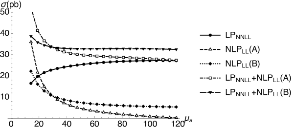
Figure 1: Dependence of the NNLL LP and LL NLP resummed Higgs production cross section on the soft scale $\mu_{s}$, for $\mu_{h}^{2}=m_{H}^{2}$. For NLP we present the result for the two cases defined in (4.6).

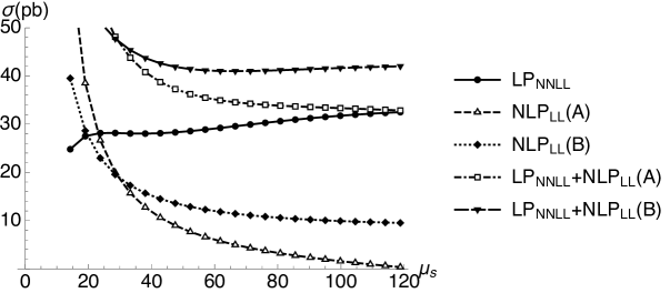
Figure 2: Same as figure 1, however using $\mu_{h}^{2}=-m_{H}^{2}$ for the hard scale.

5 Summary

In this work, we resummed all leading logarithmic corrections to the Higgs production cross section in gluon-gluon fusion, at next-to-leading power in the threshold expansion employing position-space SCET. Our main analytic result is presented in (3.11), and its expansion in powers of $\alpha_{s}$ is provided in (3.12) up to the fifth order. Our result proves that, to all orders in the strong coupling constant, the leading logarithmic terms at NLP are identical to those obtained for the threshold expansion of the Drell-Yan process in the $q\bar{q}$ channel up to an exchange of the color factor, $C_{F}\to C_{A}$. It also confirms previous conjectures about the structure of the LL resummed NLP contribution.

In addition, we explore the relevance of the resummed NLP correction for the total hadronic Higgs production cross section in proton-proton collisions at $\sqrt{s}=13$ TeV. Similarly to what has been observed at LP, a direct naive summation of the fixed-order contributions is not possible, as the sum would not converge in this case. A judicious choice of the soft scale is necessary and to that end we employ the soft scale setting procedure established in the literature for LP investigations. Even though this method may not be considered as fully systematic, it is known to provide reasonable results at LP. We find that this choice provides a series whose subsequent contributions decrease rapidly also at NLP.

We find that the LL NLP corrections are of the order of 30-40% of the NNLL LP resummed cross section (when including only leading power contributions to the latter). We also observe that the sum of NNLL LP and LL NLP contributions yields a value that is numerically close to the N³LO result, when including a resummation of $\pi^{2}$ terms in both the LP and NLP contributions. The difference between both is of similar size as the contribution to the resummed result from orders larger than or equal to $\alpha_{s}^{4}$.

As expected, the dependence of the LL NLP result on the soft scale is sizeable. Therefore, the precise numerical values should be interpreted with care. We find that the numerical results are comparable when using two different initial conditions for the soft function that are formally equivalent at LL accuracy. In conclusion, our results indicate that the NLP correction to the Higgs cross section is substantial, and it therefore appears desirable to extend NLP resummation to NLL accuracy, and eventually combine the resummed results with fixed-order computations.

Acknowledgments

We would like to thank Sven-Olaf Moch for a useful discussion. This work has been supported by the Bundesministerium für Bildung and Forschung (BMBF) grant no. 05H18WOCA1, by the D-ITP consortium, a program of NWO funded by the Dutch Ministry of Education, Culture and Science, and by Fellini - Fellowship for Innovation at INFN, funded by the European Union’s Horizon 2020 research programme under the Marie Skłodowska-Curie Cofund Action, grant agreement no. 754496.

References

• [1] C. Anastasiou, C. Duhr, F. Dulat, F. Herzog and B. Mistlberger, Higgs Boson Gluon-Fusion Production in QCD at Three Loops, Phys. Rev. Lett. 114 (2015) 212001, [1503.06056].
• [2] C. Anastasiou, C. Duhr, F. Dulat, E. Furlan, T. Gehrmann, F. Herzog et al., High precision determination of the gluon fusion Higgs boson cross-section at the LHC, JHEP 05 (2016) 058, [1602.00695].
• [3] B. Mistlberger, Higgs boson production at hadron colliders at N3LO in QCD, JHEP 05 (2018) 028, [1802.00833].
• [4] F. Dulat, B. Mistlberger and A. Pelloni, Precision predictions at N3LO for the Higgs boson rapidity distribution at the LHC, Phys. Rev. D99 (2019) 034004, [1810.09462].
• [5] S. Moch and A. Vogt, Higher-order soft corrections to lepton pair and Higgs boson production, Phys. Lett. B631 (2005) 48–57, [hep-ph/0508265].
• [6] E. Laenen and L. Magnea, Threshold resummation for electroweak annihilation from DIS data, Phys. Lett. B632 (2006) 270–276, [hep-ph/0508284].
• [7] A. Idilbi, X.-d. Ji, J.-P. Ma and F. Yuan, Threshold resummation for Higgs production in effective field theory, Phys. Rev. D73 (2006) 077501, [hep-ph/0509294].
• [8] A. Idilbi, X.-d. Ji and F. Yuan, Resummation of threshold logarithms in effective field theory for DIS, Drell-Yan and Higgs production, Nucl. Phys. B753 (2006) 42–68, [hep-ph/0605068].
• [9] V. Ahrens, T. Becher, M. Neubert and L. L. Yang, Renormalization-Group Improved Prediction for Higgs Production at Hadron Colliders, Eur. Phys. J. C62 (2009) 333–353, [0809.4283].
• [10] M. Bonvini and S. Marzani, Resummed Higgs cross section at N3LL, JHEP 09 (2014) 007, [1405.3654].
• [11] M. Beneke, A. Broggio, M. Garny, S. Jaskiewicz, R. Szafron, L. Vernazza et al., Leading-logarithmic threshold resummation of the Drell-Yan process at next-to-leading power, JHEP 03 (2019) 043, [1809.10631].
• [12] G. Sterman, Summation of Large Corrections to Short Distance Hadronic Cross-Sections, Nucl. Phys. B281 (1987) 310.
• [13] S. Catani and L. Trentadue, Resummation of the QCD Perturbative Series for Hard Processes, Nucl. Phys. B327 (1989) 323–352.
• [14] N. Bahjat-Abbas, D. Bonocore, J. Sinninghe Damsté, E. Laenen, L. Magnea, L. Vernazza et al., Diagrammatic resummation of leading-logarithmic threshold effects at next-to-leading power, 1905.13710.
• [15] E. Laenen, L. Magnea, G. Stavenga and C. D. White, Next-to-eikonal corrections to soft gluon radiation: a diagrammatic approach, JHEP 01 (2011) 141, [1010.1860].
• [16] D. Bonocore, E. Laenen, L. Magnea, S. Melville, L. Vernazza and C. D. White, A factorization approach to next-to-leading-power threshold logarithms, JHEP 06 (2015) 008, [1503.05156].
• [17] V. Del Duca, E. Laenen, L. Magnea, L. Vernazza and C. D. White, Universality of next-to-leading power threshold effects for colourless final states in hadronic collisions, JHEP 11 (2017) 057, [1706.04018].
• [18] I. Moult, I. W. Stewart, G. Vita and H. X. Zhu, First Subleading Power Resummation for Event Shapes, JHEP 08 (2018) 013, [1804.04665].
• [19] M. Beneke, M. Garny, R. Szafron and J. Wang, Anomalous dimension of subleading-power N-jet operators, JHEP 03 (2018) 001, [1712.04416].
• [20] M. Beneke, M. Garny, R. Szafron and J. Wang, Anomalous dimension of subleading-power $N$-jet operators. Part II, JHEP 11 (2018) 112, [1808.04742].
• [21] M. Beneke, M. Garny, R. Szafron and J. Wang, Violation of the Kluberg-Stern-Zuber theorem in SCET, JHEP 09 (2019) 101, [1907.05463].
• [22] C. Marcantonini and I. W. Stewart, Reparameterization Invariant Collinear Operators, Phys. Rev. D79 (2009) 065028, [0809.1093].
• [23] D. W. Kolodrubetz, I. Moult and I. W. Stewart, Building Blocks for Subleading Helicity Operators, JHEP 05 (2016) 139, [1601.02607].
• [24] I. Feige, D. W. Kolodrubetz, I. Moult and I. W. Stewart, A Complete Basis of Helicity Operators for Subleading Factorization, JHEP 11 (2017) 142, [1703.03411].
• [25] I. Moult, I. W. Stewart and G. Vita, A subleading operator basis and matching for $gg\to H$, JHEP 07 (2017) 067, [1703.03408].
• [26] M. Beneke, A. Broggio, S. Jaskiewicz and L. Vernazza, in preparation .
• [27] M. Beneke and T. Feldmann, Multipole expanded soft collinear effective theory with non-abelian gauge symmetry, Phys. Lett. B553 (2003) 267–276, [hep-ph/0211358].
• [28] C. W. Bauer, D. Pirjol and I. W. Stewart, Soft collinear factorization in effective field theory, Phys. Rev. D65 (2002) 054022, [hep-ph/0109045].
• [29] G. Bell, M. Beneke, T. Huber and X.-Q. Li, Heavy-to-light currents at NNLO in SCET and semi-inclusive $\bar{B}\to X_{s}l^{+}l^{-}$ decay, Nucl. Phys. B843 (2011) 143–176, [1007.3758].
• [30] C. Anastasiou, C. Duhr, F. Dulat, E. Furlan, T. Gehrmann, F. Herzog et al., Higgs Boson Gluon-Fusion Production Beyond Threshold in N${}^{3}LO$ QCD, JHEP 03 (2015) 091, [1411.3584].
• [31] D. de Florian, J. Mazzitelli, S. Moch and A. Vogt, Approximate N3LO Higgs-boson production cross section using physical-kernel constraints, JHEP 10 (2014) 176, [1408.6277].
• [32] M. Kramer, E. Laenen and M. Spira, Soft gluon radiation in Higgs boson production at the LHC, Nucl. Phys. B511 (1998) 523–549, [hep-ph/9611272].
• [33] N. Kidonakis, Collinear and soft gluon corrections to Higgs production at NNNLO, Phys. Rev. D77 (2008) 053008, [0711.0142].
• [34] A. Buckley, J. Ferrando, S. Lloyd, K. Nordström, B. Page, M. Rüfenacht et al., LHAPDF6: parton density access in the LHC precision era, Eur. Phys. J. C75 (2015) 132, [1412.7420].
• [35] J. Butterworth et al., PDF4LHC recommendations for LHC Run II, J. Phys. G43 (2016) 023001, [1510.03865].
• [36] S. Dulat, T.-J. Hou, J. Gao, M. Guzzi, J. Huston, P. Nadolsky et al., New parton distribution functions from a global analysis of quantum chromodynamics, Phys. Rev. D93 (2016) 033006, [1506.07443].
• [37] L. A. Harland-Lang, A. D. Martin, P. Motylinski and R. S. Thorne, Parton distributions in the LHC era: MMHT 2014 PDFs, Eur. Phys. J. C75 (2015) 204, [1412.3989].
• [38] NNPDF collaboration, R. D. Ball et al., Parton distributions for the LHC Run II, JHEP 04 (2015) 040, [1410.8849].
• [39] T. Becher, M. Neubert and G. Xu, Dynamical Threshold Enhancement and Resummation in Drell- Yan Production, JHEP 07 (2008) 030, [0710.0680].
• [40] G. Sterman and M. Zeng, Quantifying Comparisons of Threshold Resummations, JHEP 05 (2014) 132, [1312.5397].
• [41] S. Catani, M. L. Mangano, P. Nason and L. Trentadue, The Resummation of soft gluons in hadronic collisions, Nucl. Phys. B478 (1996) 273–310, [hep-ph/9604351].
• [42] S. Moch, J. A. M. Vermaseren and A. Vogt, The Quark form-factor at higher orders, JHEP 08 (2005) 049, [hep-ph/0507039].
• [43] F. Dulat, A. Lazopoulos and B. Mistlberger, iHixs 2 – Inclusive Higgs cross sections, Comput. Phys. Commun. 233 (2018) 243–260, [1802.00827].