High-dimensional sample covariance matrices with Curie-Weiss entries

Abstract.

We study the limiting spectral distribution of sample covariance matrices $XX^{T}$, where $X$ are $p\times n$ random matrices with correlated entries, for the cases $p/n\to y\in[0,\infty)$. If $y>0$, we obtain the Marčenko–Pastur distribution and in the case $y=0$ the semicircle distribution (after appropriate rescaling). The entries we consider are Curie-Weiss spins, which are correlated random signs, where the degree of the correlation is governed by an inverse temperature $\beta>0$. The model exhibits a phase transition at $\beta=1$. The correlation between any two entries decays at a rate of $O(np)$ for $\beta\in(0,1)$, $O(\sqrt{np}$) for $\beta=1$, and for $\beta>1$ the correlation does not vanish in the limit. In our proofs we use Stieltjes transforms and concentration of random quadratic forms.

1. Introduction and Preliminaries

In many contemporary applications, one is faced with large data sets where both the dimension of the observations and the sample size are large. In quantum mechanics, for example, the energy levels of particles in a large system can be approximated by the eigenvalues of a large random matrix. Estimating the underlying covariance structure of high-dimensional data with the sample covariance matrix can be misleading [3, 10]. Even in the case of independent covariates, it is well-known that the sample covariance matrix poorly estimates the population covariance matrix. The fluctuations of the off-diagonal entries of the sample covariance matrix aggregate, creating an estimation bias which was quantified in 1967 by the famous Marčenko–Pastur theorem [23]. Ever since, the classical setting of well-behaved i.i.d. ensembles was extended to investigate settings more aligned with reality. In many situations, it is reasonable to assume that entries in data sets are dependent. The dependence might span between different observations, but also between covariates of individual observations. In random matrix theory, one often considers models exhibiting linear dependence between the entries. Works that consider non-linear dependencies are sparse. The paper [4], for example, incorporates non-linear dependence within the columns of the data matrix, but assumes these columns to be independent. In this paper, we consider a data matrix filled with Curie-Weiss spins. This model exhibits nonlinear dependence between all entries. For technical reasons, settings with correlated entries are harder to analyze, since many proof techniques break down in presence of correlations.

Another way to deviate from the classical setting is to assume that data might stem from heavy-tailed distributions. The theory for the eigenvalues and eigenvectors of the sample covariance matrices stemming from heavy-tailed time series with infinite fourth moment is quite different from the classical Marčenko–Pastur theory which applies in the light-tailed case. For detailed discussions about classical random matrix theory, we refer to the monographs [3, 27], while the developments in the heavy-tailed case can be found in [8, 9, 17, 1, 16, 18] and the references therein.

The Marčenko–Pastur law gives insight into the spectrum of large dimensional sample covariance matrices. Assume we have $n$ observations $x_{1},\ldots,x_{n}$, each with $p$ real-valued covariates, where $n,p\in\mathbb{N}$, so that $x_{i}=(x_{i}(1),\ldots,x_{i}(p))^{T}$ for all $i\in\{1,\ldots,n\}$. Define the $p\times n$ data matrix $X_{n}\mathrel{\vbox{\hbox{\scriptsize.}\hbox{\scriptsize.}}}=(x_{1},x_{2},\ldots,x_{n})$, that is, $X_{n}$ has columns $x_{i}$. The (centered) sample covariance matrix is then defined by

$$\tilde{V}_{n}\mathrel{\vbox{\hbox{\scriptsize.}\hbox{\scriptsize.}}}=\frac{1}{n-1}\sum_{k=1}^{n}(x_{k}-\bar{x})(x_{k}-\bar{x})^{T},$$

which is of dimension $p\times p$. Here, the vector $\bar{x}$ denotes the arithmetic mean of the vectors $x_{k}$. Assuming that the data stems from $n$ i.i.d. realizations of an $\mathbb{R}^{p}$-valued random vector $x$ with $\mathcal{L}_{2}$-entries, $\tilde{V}_{n}$ is an unbiased estimator for its covariance matrix ${\rm var}(x)$.

The sample covariance matrix is of crucial importance in multivariate statistics, for instance in principal component analysis, canonical correlation analysis, multivariate regression, factor analysis, hypothesis testing and discriminant analysis. Many test statistics are based on the eigenvalues of the sample covariance matrix. Examples include independence tests [7] and likelihood ratio tests. For the latter it is essential that the log-determinant of $\tilde{V}_{n}$ can be written as $\log(\lambda_{1})+\cdots+\log(\lambda_{p})$, where $(\lambda_{i})$ are the eigenvalues of $\tilde{V}_{n}$.

When analyzing the limiting spectral distribution (LSD) of the eigenvalues, it suffices to consider the (non-centered) sample covariance matrix

$$V_{n}\mathrel{\vbox{\hbox{\scriptsize.}\hbox{\scriptsize.}}}=\frac{1}{n}\sum_{k=1}^{n}x_{k}x_{k}^{T}=\frac{1}{n}X_{n}X_{n}^{T},$$ (1)

since $\bar{x}\bar{x}^{T}$ is of rank $1$, see Theorem A.44 in [3]. From now on we will refer to $V_{n}$ as the sample covariance matrix. Our object of interest in this paper will be the limit of the empirical spectral distributions (ESD) $F_{V_{n}}$ defined as

$$F_{V_{n}}(x)=\frac{1}{p}\;\sum_{i=1}^{p}\mathds{1}_{\{\lambda_{i}(V_{n})\leq x\}},\qquad x\in\mathbb{R}\,,$$

where $\lambda_{1}(V_{n})\geq\cdots\geq\lambda_{p}(V_{n})$ are the ordered eigenvalues of $V_{n}$. If such a limit exists in the sense of weak convergence almost surely, we call it the limiting spectral distribution of $V_{n}$.

Also, we will assume that the number of covariates $p$ and the sample size $n$ are large and tend to infinity together. In this paper, the sample size $n$ is a function of the dimension $p$ (cf. Remark rem:npdependence) and the dimension increases at most proportionally to the sample size. To be precise, we assume

$$n=n_{p}\to\infty\quad\text{ and }\quad\frac{p}{n_{p}}\to y\in[0,\infty)\,,\quad\text{ as }p\to\infty\,.$$ (2)

The constant $y$ controls the growth of the dimension relative to the sample size. Most of the random matrix literature focuses exclusively on the case $y>0$, while the case $y=0$ plays only a minor role. In many fields, however, the wider range of possible growth rates arising in the $y=0$ regime is desirable. The framework in this paper unifies these two lines of research.

1.1. Background

Before we present our model, we provide some background. Assume that the entries of $X_{n}$ are i.i.d. with unit variance and zero mean. Then if $p/n\to y\in(0,\infty)$ the limiting spectral distribution of $(V_{n})$ is the so-called Marčenko–Pastur distribution $\mu^{y}$. The (standard) MP distribution with ratio index $y\in(0,\infty)$ is the probability measure $\mu^{y}$ on $(\mathbb{R},\mathcal{B})$ given by

$$\mu^{y}=\frac{1}{2\pi xy}\sqrt{((1+\sqrt{y})^{2}-x)(x-(1-\sqrt{y})^{2})}\mathds{1}_{((1-\sqrt{y})^{2},(1+\sqrt{y})^{2})}(x)\lambda(\text{d}x)+\left(1-\frac{1}{y}\right)\delta_{0}\mathds{1}_{y>1},$$

where $\lambda$ denotes the Lebesgue measure on $(\mathbb{R},\mathcal{B})$ and $\delta_{0}$ denotes the Dirac measure in $0$.

It is well-known that measures on $\mathbb{R}$ are uniquely characterized by their Stieltjes transforms [27]. The Stieltjes transform of $\mu^{y}$ is given for $z\in\mathbb{C}_{+}=\{c\in\mathbb{C}:\operatorname{Im}(c)>0\}$ by

$$S_{\mu^{y}}(z):=\int_{\mathbb{R}}\frac{1}{x-z}\mu^{y}(dx)=\frac{1-y-z+\sqrt{(1-y-z)^{2}-4yz}}{2yz},$$

where throughout this paper, if $z\in\mathbb{R}_{+}$, $\sqrt{z}$ denotes the positive square root, while if $z\in\mathbb{C}\backslash\mathbb{R}_{+}$, then $\sqrt{z}$ denotes the complex square root with positive imaginary part; see for example [3]. If $p/n\to\infty$, we observe $\delta_{0}$ as LSD of $V_{n}$, as there are at most $\min(p,n)$ positive eigenvalues of $V_{n}$.

In the case $p/n\to 0$, the limiting spectral distribution of $V_{n}$ is the Dirac measure at $1$. After centering $V_{n}$ by the identity matrix $I$ and a subsequent appropriate rescaling, one can obtain a non-degenerate limiting spectral distribution. In [2] it is proved under the additional assumption $\mathds{E}[X_{n}(1,1)^{4}]<\infty$ that the empirical spectral distribution of the matrices $\sqrt{n/p}\,(V_{n}-I)$ converges to the semicircle law $G$ with Lebesgue density

$$g(x)=\tfrac{1}{2\pi}\sqrt{4-x^{2}}\mathds{1}_{[-2,2]}(x)\,,\qquad x\in\mathbb{R},$$

and Stieltjes transform

$$s_{G}(z)=\frac{-z+\sqrt{z^{2}-4}}{2}\,,\qquad z\in\mathbb{C}_{+}.$$

The i.i.d. assumption on the entries of the data matrix $X_{n}$ can be relaxed to linear dependence of the form $\Sigma_{n}^{1/2}X_{n}$ for symmetric positive definite deterministic matrices $\Sigma_{n}$ with uniformly bounded spectral or operator norm $\|\Sigma_{n}\|:=\sqrt{\lambda_{1}(\Sigma_{n}\Sigma_{n}^{T})}$. For $p/n\to y>0$, the Stieltjes transform of the LSD of $n^{-1}\Sigma_{n}^{1/2}X_{n}X_{n}^{T}\Sigma_{n}^{1/2}$ can then be characterized via the LSD of $\mathds{E}[V_{n}]=\Sigma_{n}$; see [3] for details. The same holds in the case $p/n\to 0$ for the LSD of $\sqrt{n/p}\,(n^{-1}\Sigma_{n}^{1/2}X_{n}X_{n}^{T}\Sigma_{n}^{1/2}-\Sigma_{n})$ as proved in [24] and [26].

It is important to note that the linear dependence between the entries of $X_{n}$ was a crucial assumption for the above results. For nonlinear dependencies the situation becomes more delicate as the following examples will show. We present two examples of random matrices $Y_{n}$ with dependent entries and $\mathds{E}[n^{-1}Y_{n}Y_{n}^{T}]=I$ for which the LSD of $n^{-1}Y_{n}Y_{n}^{T}$ is not the Marčenko–Pastur distribution $\mu^{y}$.

Example 1.

Assume that the entries of $X_{n}$ are i.i.d. continuous random variables with unit variance, zero mean and let $p/n\to y>0$. Kendall’s Tau is a U-statistic which measure the association of random variables. For higher dimensional observations, such as the columns $x_{i}=(x_{i}(1),\ldots,x_{i}(p))^{T}$ of the data matrix $X$, the (empirical) Kendall’s Tau matrix is defined as

$$\tau_{n}=\tfrac{2}{n(n-1)}\sum_{1\leq s<t\leq n}\operatorname{sign}(x_{s}-x_{t})(\operatorname{sign}(x_{s}-x_{t}))^{T}\,,$$

where $\operatorname{sign}$ of a vector is taken coordinatewise. In particular, one sees that $\tau_{n}(i,i)=1$. Since $X_{n}$ has i.i.d. continuous entries, we have $\mathds{E}[\tau_{n}]=I$. Bandeira et al. [5] proved that the empirical spectral distribution $F_{\tau_{n}}$ of $\tau_{n}$ converges, namely

$$F_{\tau_{n}}\stackrel{{\scriptstyle\mathds{P}}}{{\rightarrow}}\tfrac{2}{3}\,\xi+\tfrac{1}{3}\,,\quad p\to\infty\,,$$

where the random variable $\xi$ has a Marčenko–Pastur distribution with parameter $y$. In Theorem 5 we will observe a similar scaling phenomenon. The exact formula for $Y_{n}$ such that $n^{-1}Y_{n}Y_{n}^{T}=\tau_{n}$ can be found in [6].

Example 2.

Assume that the entries of $X_{n}$ are i.i.d. symmetric random variables with tails $\mathds{P}(|x_{1}(1)|>t)=t^{-\alpha}\ell(t)$, where $\alpha\in(0,2)$ and $\ell$ is a slowly varying function at infinity. Under the regime $p/n\to y>0$, set $V_{n}=n^{-1}X_{n}X_{n}^{T}$ and consider the sample correlation matrices

$$R_{n}=(\operatorname{diag}(V_{n}))^{-1/2}V_{n}(\operatorname{diag}(V_{n}))^{-1/2}\,.$$

It was shown in [16] that $\mathds{E}[R_{n}]=I$. However, from [16, Theorem 3.1 part (2)] we know that

$$\liminf_{n\to\infty}\mathds{E}\Big{[}\int x^{k}F_{R_{n}}(dx)\Big{]}>\beta_{k}(y)\,,\qquad k\geq 4\,,$$

where $\beta_{k}(y)$ is the $k$-th moment of the Marčenko–Pastur law $\mu^{y}$. Since $\mu^{y}$ is uniquely characterized by its moments, the LSD of $R_{n}$ cannot be $\mu^{y}$.

1.2. Our model

We will consider a data matrix $X_{n}$ with correlated entries. To this end, we introduce the Curie-Weiss model which is an exactly solvable model of ferromagnetism. “Because of its simplicity and because of the correctness of at least of some of its predictions, the Curie-Weiss model occupies an important place in the statistical mechanics literature and its application to information theory [22].” The first time that random matrices with Curie-Weiss spins were analyzed was in [15], with subsequent improvements in [19, 21, 14, 12], where the last two publications are based on [11]. All of these texts were concerned with Wigner type matrices and convergence to the semicircle distribution.

Definition 3.

Let $n\in\mathbb{N}$ be arbitrary and $Y_{1},\ldots,Y_{n}$ be random variables defined on some probability space $(\Omega,\mathcal{A},\mathds{P})$. Let $\beta>0$, then we say that $Y_{1},\ldots,Y_{n}$ are Curie-Weiss($\beta$,$n$)-distributed, if for all $y_{1},\ldots,y_{n}\in\{-1,1\}$ we have that

$$\mathds{P}(Y_{1}=y_{1},\ldots,Y_{n}=y_{n})=\frac{1}{Z_{\beta,n}}\cdot\operatorname{e}^{\frac{\beta}{2n}\left(\sum_{i=1}^{n}y_{i}\right)^{2}}\,,$$

where $Z_{\beta,n}=\sum_{y_{1},\ldots,y_{n}\in\{-1,1\}}\operatorname{e}^{\frac{\beta}{2n}\left(\sum_{i=1}^{n}y_{i}\right)^{2}}$ is a normalization constant. The parameter $\beta$ is called inverse temperature.

Note that in above definition, $(Y_{1},\ldots,Y_{n})$ is an exchangeable random vector, since the probability of any spin configuration $(y_{1},\ldots,y_{n})$ only depends on the sum of the spins. The Curie-Weiss($\beta,n$) distribution is used to model the behavior of $n$ ferromagnetic particles (spins) at the inverse temperature $\beta$. At low temperatures (if $\beta$ is large), all magnetic spins are likely to have the same alignment, resembling a strong magnetic effect. On the contrary, at high temperatures (if $\beta$ is small), spins can act almost independently, resembling a weak magnetic effect. The model exhibits a phase transition at $\beta=1$, meaning that the behavior of the distribution varies significantly in the realms $\beta\in(0,1)$, $\beta=1$ and $\beta>1$. To exemplify a manifestation of this phase transition, we formulate the following result; see Theorem 5.17 in [20].

Lemma 4.

Fix $l\in\mathbb{N}$ and let for all $n\geq l$, $(Y^{(n)}_{1},\ldots,Y^{(n)}_{l})$ be part of a Curie-Weiss($\beta,n$) distributed random vector. If $l$ is even, the following statements hold:

1. If $\beta<1$, then for some constant $c(\beta,l)>0$, $\mathds{E}Y^{(n)}_{1}\cdots Y^{(n)}_{l}\sim c(\beta,l)n^{-l/2}$ as $n\to\infty$.

2. If $\beta=1$, then for some constant $c(l)>0$, $\mathds{E}Y^{(n)}_{1}\cdots Y^{(n)}_{l}\sim c(l)n^{-l/4}$ as $n\to\infty$.

3. If $\beta>1$, then $\mathds{E}Y^{(n)}_{1}\cdots Y^{(n)}_{l}\sim m^{l}$ as $n\to\infty$, where $m\in(0,1)$ is the unique positive number such that $\tanh(\beta m)=m$.

If $l$ is odd, then for all $\beta>0$ one has $\mathds{E}Y^{(n)}_{1}\cdots Y^{(n)}_{l}=0$.

Note that in the setting of Lemma 4, the correlation $\mathds{E}Y^{(n)}_{1}Y^{(n)}_{2}$ is of a different order for the three regions of $\beta$. If $\beta<1$, the correlation $\mathds{E}Y^{(n)}_{1}Y^{(n)}_{2}$ decays at a rate of $n^{-1}$. For the critical temperature $\beta=1$ the decay rate is $n^{-1/2}$ , whereas if $\beta>1$, the correlation $\mathds{E}Y^{(n)}_{1}Y^{(n)}_{2}$ converges to $m^{2}$ and hence does not vanish as $n\to\infty$. In our main result Theorem 5, we will see that for $\beta>1$ a different normalization of the sample covariance matrix is required to account for the correlation at level $m^{2}$.

Objective and structure of this paper

The aim of this paper is to characterize the LSD of the sample covariance matrices $V_{n}=n^{-1}X_{n}X_{n}^{T}$, where $X_{n}$ follows a Curie-Weiss distribution. At the critical temperature $\beta=1$ a phase transition occurs. In Section 2, we see that the LSD is a possibly rescaled Marčenko–Pastur or semicircle distribution. Section 3 contains some useful lemmas and the proof of our main result.

Notation

For simplicity of notation, we define for all $n\in\mathbb{N}$: $[{n}]\mathrel{\vbox{\hbox{\scriptsize.}\hbox{\scriptsize.}}}=\{1,\ldots,n\}$. Further, whenever there is no ambiguity about the dimension we denote the identity matrix by $I$.

2. Main result

Our main result characterizes the limiting spectral distributions of sample covariance matrices with Curie-Weiss entries with parameter $\beta>0$ in the regimes $p/n\to y>0$ and $p/n\to 0$.

Theorem 5.

Assume (2) and that the entries of the $p\times n$ matrix $X_{n}$ are Curie-Weiss$(\beta,np)$ distributed with $\beta>0$, where we assume that $(X_{n}(i,j))_{i\in[p],j\in[n]}$ are defined on a common probability space. Denote by $F_{n}$ the ESD of $V_{n}\mathrel{\vbox{\hbox{\scriptsize.}\hbox{\scriptsize.}}}=n^{-1}X_{n}X_{n}^{T}$.

• Assume $\beta\in(0,1]$. If $p/n\to y\in(0,\infty)$, then $(F_{n})_{n}$ converge weakly almost surely to the Marčenko–Pastur distribution $\mu^{y}$, as $p\to\infty$. If $p/n\to 0$, then the ESDs of $\sqrt{\tfrac{n}{p}}(V_{n}-I)$ converge weakly almost surely to the semicircle distribution $G$, as $p\to\infty$.

• Assume $\beta\in(1,\infty)$ and let $m$ be the unique number in $(0,1)$ satisfying $\tanh(m\beta)=m$. If $p/n\to y\in(0,\infty)$, then the ESDs of $(1-m^{2})^{-1}V_{n}$ converge weakly almost surely to the Marčenko–Pastur distribution $\mu^{y}$, as $p\to\infty$. If $p/n\to 0$, then the ESDs of $\sqrt{\frac{n}{p}}\left(\frac{1}{1-m^{2}}V_{n}-I\right)$ converge weakly almost surely to the semicircle distribution $G$, as $p\to\infty$.

By Lemma 4, the correlations between the entries of $X_{n}$ increase with the value $\beta$. Theorem 5 shows that for $\beta\leq 1$ the correlation is still weak enough to not affect the LSD, in the sense that we obtain the same LSD as for a sample of i.i.d. random variables. For $\beta>1$ the asymptotic behavior of the correlations changes drastically. Consequently, a different normalization of the sample covariance matrix is required to account for the correlation at constant level $m^{2}$.

Remark 6.

The convergence in Theorem 5 is for $p\to\infty$, which is standard in the $p/n\to 0$ literature; see for example [2, 24, 26]. If there exists a $\delta>0$ such that $n^{\delta}/p\to 0$, the convergence also holds for $n\to\infty$; compare also with [10, Corollary 2]. Indeed, $n^{\delta}/p\to 0$ for some $\delta>0$ is equivalent to $p_{n}^{-a}$ being summable over $n$ for some large $a>0$, which is required for the Borel-Cantelli argument in the proof of Theorem 5. Our formulation with $p\to\infty$ is slightly more flexible because it also allows choices such as $p=\log n$.

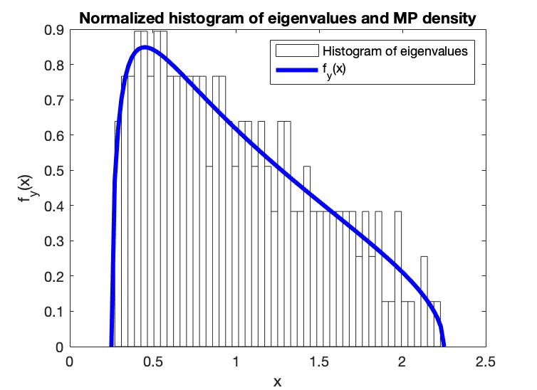
Figure 1. Simulation for $(p,n)=(200,800)$ and $\beta=0.5$. In blue: Density $f_{1/4}$. Histogram: Eigenvalues of $n^{-1}X_{n}X_{n}^{T}$.

In Figure 1 and Figure 2, we can see a simulation output where a $200\times 800$ random matrix with Curie-Weiss entries was simulated, using the Metropolis algorithm with $16\cdot 10^{6}$ steps. We compare the histogram of the eigenvalues with the Marčenko–Pastur density $f_{p/n}$,

$$f_{y}(x)=\frac{1}{2\pi xy}\sqrt{((1+\sqrt{y})^{2}-x)(x-(1-\sqrt{y})^{2})}\mathds{1}_{((1-\sqrt{y})^{2},(1+\sqrt{y})^{2})}(x)\,,\qquad x\in\mathbb{R},y\in(0,1]\,.$$

While in Figure 1, the ensemble was simulated for $\beta=0.5$, in Figure 2 we used $\beta=1.29727$, so that $\tanh(\beta m)=m$ holds for $m=3/4$. The largest eigenvalue of $n^{-1}XX^{T}$ resp. $(n(1-m^{2}))^{-1}$ was roughly $113$ resp. $258$ and was excluded from the histogram in Figure 2.

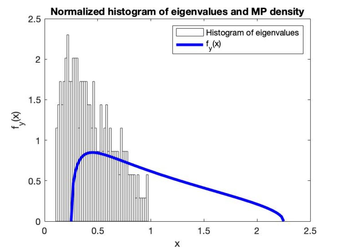
Figure 2. Simulation for $(p,n)=(200,800)$ and $\beta=1.29727$. In blue: Density $f_{1/4}$. Left histogram: Eigenvalues of $n^{-1}X_{n}X_{n}^{T}$. Right histogram: Eigenvalues of $(n(1-m^{2}))^{-1}X_{n}X_{n}^{T}$, where $m=3/4$, so that $\tanh(\beta m)=m$.

In the proof of Theorem 5, we use techniques developed in [12] and [13]. An important tool is the fact that Curie-Weiss($\beta,n$) spins $(Y_{1},\ldots,Y_{n})$ are conditionally i.i.d. That is, without loss of generality we can assume that they are defined on the same probability space as a Lebesgue-continuous mixing variable $M^{\beta}_{n}$ with support $[-1,1]$, such that conditioned on $M^{\beta}_{n}=t\in(-1,1)$, $(Y_{1},\ldots,Y_{n})$ are i.i.d. $P_{t}$-distributed, where $P_{t}$ is the probability measure on $\{\pm 1\}$ with

$$P_{t}(1)=\frac{1+t}{2}\qquad\text{and}\qquad P_{t}(-1)=\frac{1-t}{2}.$$

Next, we collect some properties of the mixing variable $M_{n}^{\beta}$ in the following lemma which is taken from [20]; see Theorem 5.6, Remark 5.7, Proposition 5.9 and Theorem 5.17 therein.

Lemma 7.

If $Y=(Y_{1},\ldots,Y_{n})$ are Curie-Weiss($\beta$,$n$)-distributed for some $\beta>0$ and $n\in\mathbb{N}$, then w.l.o.g. there exists a random variable $M^{\beta}_{n}$ supported on $[-1,1]$ with the following properties.

1. The distribution of $M^{\beta}_{n}$ has Lebesgue-density $f^{\beta}_{n}$,

   $$f^{\beta}_{n}(t)\mathrel{\vbox{\hbox{\scriptsize.}\hbox{\scriptsize.}}}=\frac{1}{\int_{(-1,1)}\frac{e^{-\frac{n}{2}F_{\beta}(s)}}{1-s^{2}}\lambda(\text{d}s)}\frac{e^{-\frac{n}{2}F_{\beta}(t)}}{1-t^{2}}\mathds{1}_{(-1,1)}(t)\,,\qquad t\in(-1,1),$$

   where for all $s\in(-1,1)$ we define

   $$F_{\beta}(s)\mathrel{\vbox{\hbox{\scriptsize.}\hbox{\scriptsize.}}}=\frac{1}{\beta}\left(\frac{1}{2}\ln\left(\frac{1+s}{1-s}\right)\right)^{2}+\ln(1-s^{2}).$$

2. $\mathds{P}^{M^{\beta}_{n}}$-almost surely, $\mathds{P}^{Y|M^{\beta}_{n}=t}=\otimes_{i\in[{n}]}\mathds{P}^{Y_{i}|M^{\beta}_{n}=t}=\otimes_{i\in[{n}]}P_{t}$. In words, conditionally on $M_{n}^{\beta}$ the $Y_{1},\ldots,Y_{n}$ are i.i.d. $P_{t}$-distributed random variables.

3. If $\beta<1$, the mixing variable $M^{\beta}_{n}$ satisfies the following moment decay:

   $$\forall\leavevmode\nobreak\ a\in 2\mathbb{N}:\int_{[-1,+1]}t^{a}\mathds{P}^{M^{\beta}_{n}}(\text{d}t)\leq\frac{K_{\beta,a}}{n^{\frac{a}{2}}}.$$

4. If $\beta=1$, the mixing variable $M^{\beta}_{n}$ satisfies the following moment decay:

   $$\forall\leavevmode\nobreak\ a\in 2\mathbb{N}:\int_{[-1,+1]}t^{a}\mathds{P}^{M^{\beta}_{n}}(\text{d}t)\leq\frac{K_{\beta,a}}{n^{\frac{a}{4}}},$$

where $K_{\beta,a}\in\mathbb{R}_{+}$ are constants that depend on $\beta$ and $a$ only.

In the case $\beta>1$ we will work with suitably restandardized Curie-Weiss spins in order to use the following lemma which can be found in [13].

Lemma 8.

Let $(Y_{1},\ldots,Y_{n})$ be Curie-Weiss($\beta,n$)-distributed with $\beta>1$ and mixing variable $M^{\beta}_{n}$. Denote by $m\in(0,1)$ the unique positive number satisfying $\tanh(m\beta)=m$. For $i\in\{1,\ldots,n\}$ define

$$Z_{i}\mathrel{\vbox{\hbox{\scriptsize.}\hbox{\scriptsize.}}}=\frac{1}{\sqrt{1-m^{2}}}\big{(}Y_{i}-m\mathds{1}_{M^{\beta}_{n}>0}+m\mathds{1}_{M^{\beta}_{n}<0}\big{)}.$$

Then $(Y_{1},\ldots,Y_{n})$ are conditionally i.i.d. given $M^{\beta}_{n}$ and the following statements hold.

1. Almost surely, $(Y_{1},\ldots,Y_{n})$ takes values in $\{\frac{\pm 1+m}{\sqrt{1-m^{2}}}\}^{n}\cup\{\frac{\pm 1-m}{\sqrt{1-m^{2}}}\}^{n}$.

2. For each $i\in\{1,\ldots,n\}$,

   $$\mathds{E}(Z_{i}|M^{\beta}_{n}=t)=\zeta(t) \mathrel{\vbox{\hbox{\scriptsize.}\hbox{\scriptsize.}}}=\begin{cases}\frac{1}{\sqrt{1-m^{2}}}(t-m),&\quad t>0,\\ \frac{1}{\sqrt{1-m^{2}}}(t+m),&\quad t<0,\end{cases}$$

   $$\mathds{E}(1-Z^{2}_{i}|M^{\beta}_{n}=t)=\psi(t) \mathrel{\vbox{\hbox{\scriptsize.}\hbox{\scriptsize.}}}=\begin{cases}\frac{2m}{1-m^{2}}(t-m),&\quad t>0,\\ \frac{2m}{1-m^{2}}(t+m),&\quad t<0.\end{cases}$$

3. We obtain the following bounds on the moments of $\zeta(M^{\beta}_{n})$ and $\psi(M^{\beta}_{n})$:

   $$\forall\leavevmode\nobreak\ a\in 2\mathbb{N}: \int_{[-1,+1]}|{\zeta(t)}|^{a}\mathds{P}^{M^{\beta}_{n}}(\text{d}t)\leq\frac{K_{\beta,a}}{n^{\frac{a}{2}}},$$

   $$\forall\leavevmode\nobreak\ a\in 2\mathbb{N}: \int_{[-1,+1]}|{\psi(t)}|^{a}\mathds{P}^{M^{\beta}_{n}}(\text{d}t)\leq\frac{K_{\beta,a}}{n^{\frac{a}{2}}}.$$

Here, the constants $K_{\beta,a}>0$ depend only on $\beta$ and $a$.

3. Proof of Theorem 5

We will prove the cases $\beta\leq 1$ and $\beta>1$ separately, but before we begin, we will provide two lemmas which we will use throughout the proof. The first lemma is taken from [12], see their Theorem 39.

Lemma 9.

Let $n\in\mathbb{N}$ be arbitrary, $(a_{i,j})_{i,j\in[{n}]}$ and $(b_{i})_{i\in[{n}]}$ be deterministic complex numbers, $(Y_{i})_{i\in[{n}]}$ be independent and complex-valued random variables with common expectation $t\in\mathbb{C}$. Further, we assume that for all $a\geq 2$ there exists a $\mu_{a}\in\mathbb{R}_{+}$ such that $\|Y_{i}-t\|_{a}:=\mathds{E}[|Y_{i}-t|^{a}]^{1/a}\leq\mu_{a}$ for all $i\in[{n}]$. Then we obtain for all $a\geq 2$:

$$i) \quad\left\|\sum\limits_{i\in[{n}]}b_{i}Y_{i}\right\|_{a}\leq\left(A_{a}\mu_{a}+\sqrt{n}|{t}|\right)\sqrt{\sum\limits_{i\in[{n}]}|{b_{i}}|^{2}}\,,$$

$$ii) \quad\left\|\sum\limits_{\begin{subarray}{c}i,j\in[{n}]\\ i\neq j\end{subarray}}a_{i,j}Y_{i}Y_{j}\right\|_{a}\leq A_{a}\mu_{a}|{t}|\sqrt{\sum_{j\in[{n}]}\left|{\sum_{i\in[{n}]\backslash\{j\}}a_{i,j}}\right|^{2}}+A_{a}\mu_{a}|{t}|\sqrt{\sum_{i\in[{n}]}\left|{\sum_{j\in[{n}]\backslash\{i\}}a_{i,j}}\right|^{2}}$$

$$\quad+4A_{a}^{2}\mu^{2}_{a}\sqrt{\sum\limits_{\begin{subarray}{c}i,j\in[{n}]\\ i\neq j\end{subarray}}|{a_{i,j}}|^{2}}+|{t}|^{2}\left|\sum\limits_{\begin{subarray}{c}i,j\in[{n}]\\ i\neq j\end{subarray}}a_{i,j}\right|\leq\left(4A_{a}^{2}\mu^{2}_{a}+2A_{a}\mu_{a}\sqrt{n}|{t}|+n|{t}|^{2}\right)\sqrt{\sum\limits_{\begin{subarray}{c}i,j\in[{n}]\\ i\neq j\end{subarray}}|{a_{i,j}}|^{2}}\,,$$

where $A_{a}\in\mathbb{R}_{+}$ is positive constant depending only on $a$.

Proof.

See [12]. ∎

The following lemma allows us to apply Lemma 9 to the setting we will encounter in our proof.

Lemma 10.

Let $X$ be a $p\times n$ matrix with real-valued entries, $z\in\mathbb{C}_{+}$. Define

$$F(X)\mathrel{\vbox{\hbox{\scriptsize.}\hbox{\scriptsize.}}}=X^{T}\left(\frac{1}{n}XX^{T}-z\right)^{-1}X.$$ (3)

Then we obtain the following bounds:

$$i)\quad\sqrt{\sum_{i\neq j}^{n}|{F_{ij}(X)}|^{2}}\leq n\sqrt{p}\left(1+\frac{|{z}|}{\operatorname{Im}(z)}\right)\,,\qquad ii)\quad|{\operatorname{tr}F(X)}|\leq np\left(1+\frac{|{z}|}{\operatorname{Im}(z)}\right).$$

Further, if all entries in $X$ are uniformly bounded by some $b>0$, we obtain:

$$iii)\quad\left|{\sum_{i,j\in[{n}]}F_{ij}(X)}\right|\leq\frac{b^{2}p}{\operatorname{Im}(z)}+\frac{1}{n}\left(1+\frac{|z|}{\operatorname{Im}(z)}\right),\qquad iv)\quad\forall\,j\in[{n}]:\left|{\sum_{i\in[{n}]\backslash\{j\}}F_{ij}(X)}\right|\leq\frac{b^{2}p}{n\operatorname{Im}(z)}.$$

Proof.

To prove i), we recall that

1. $\text{Spectrum}(X^{T}(XX^{T}-z)^{-1}X)\cup\{0\}=\text{Spectrum}((XX^{T}-z)^{-1}XX^{T})\cup\{0\}$,

2. $(XX^{T}-z)^{-1}XX^{T}=I+z(XX^{T}-z)^{-1}$,

and that $\|\cdot\|_{F}\leq\sqrt{m}\|\cdot\|$ for $m\times m$ matrices, where $\|\cdot\|_{F}$ denotes the Frobenius norm and $\|\cdot\|$ denotes the operator norm. Therefore,

$$\sqrt{\sum_{i\neq j}^{n}|{F_{ij}(X)}|^{2}} \leq\sqrt{\sum_{i\neq j}^{n}\left|{\left[X^{T}\left(\frac{1}{n}XX^{T}-z\right)^{-1}X\right](i,j)}\right|^{2}}=n\left\|\frac{1}{n}X^{T}\left(\frac{1}{n}XX^{T}-z\right)^{-1}X\right\|_{F}$$

$$=n\left\|\left(\frac{1}{n}XX^{T}-z\right)^{-1}\left(\frac{1}{n}XX^{T}\right)\right\|_{F}=n\left\|I_{p-1}+z\left(\frac{1}{n}XX^{T}-z\right)^{-1}\right\|_{F}$$

$$\leq n\sqrt{p}\left\|I_{p-1}+z\left(\frac{1}{n}XX^{T}-z\right)^{-1}\right\|\leq n\sqrt{p}\left(1+\frac{|z|}{\operatorname{Im}(z)}\right).$$

For ii) we calculate

$$\begin{split}&|{\operatorname{tr}F(X)}|=n\left|{\operatorname{tr}\left(\left(\frac{1}{n}XX^{T}-z\right)^{-1}\left(\frac{1}{n}XX_{n}^{T}\right)\right)}\right|\\ &\leq np\left\|\left(\frac{1}{n}XX^{T}-z\right)^{-1}\left(\frac{1}{n}XX^{T}\right)\right\|\leq np\left(1+\frac{|{z}|}{\operatorname{Im}(z)}\right),\end{split}$$

where the last step follows as in the proof of i). This shows ii). For iii) let $1_{n}\mathrel{\vbox{\hbox{\scriptsize.}\hbox{\scriptsize.}}}=(1,\ldots,1)^{T}\in\mathbb{R}^{n}$ and $Y\mathrel{\vbox{\hbox{\scriptsize.}\hbox{\scriptsize.}}}=n^{-1/2}X$. Then we see that

$$\begin{split}n&\left|{\sum_{i,j\in[{n}]}F_{ij}(X)}\right|=\left|{1_{n}^{T}Y^{T}(YY^{T}-z)^{-1}Y1_{n}}\right|\\ &\leq\left|{1_{n}^{T}Y^{T}\left[(YY^{T}-z)^{-1}-(YY^{T}+Y1_{n}1_{n}^{T}Y^{T}-z)^{-1}\right]Y1_{n}}\right|\\ &\quad+\left|{1_{n}^{T}Y^{T}(YY^{T}+Y1_{n}1_{n}^{T}Y^{T}-z)^{-1}Y1_{n}}\right|=:P_{1}+P_{2}\,.\end{split}$$

By [25, Lemma 2.6], one has

$$P_{1}\leq\frac{\|Y1_{n}1_{n}^{T}Y^{T}\|}{\operatorname{Im}(z)}=\frac{|{1_{n}^{T}Y^{T}Y1_{n}}|}{\operatorname{Im}(z)}=\frac{1}{\operatorname{Im}(z)}\left|{\frac{1}{n}\sum_{i\in[{n}]}\sum_{j\in[{p}]}\sum_{s\in[{n}]}X_{ij}X_{js}}\right|\leq\frac{b^{2}np}{\operatorname{Im}(z)}\,.$$

To bound $P_{2}$, recall from [28] that for a real, symmetric, positive semidefinite $m\times m$ matrix $M$; $x\in\mathbb{R}^{m}$, $z\in\mathbb{C}_{+}$ the following inequality holds:

$$\left|{x^{T}(M+xx^{T}-z)^{-1}x}\right|\leq 1+\frac{|z|}{\operatorname{Im}(z)}\,.$$ (4)

So in particular $P_{2}$ is bounded by the r.h.s. of (4). This yields the bound

$$\left|{\sum_{i,j\in[{n}]}F_{ij}(X)}\right|\leq\frac{P_{1}+P_{2}}{n}\leq\frac{b^{2}p}{\operatorname{Im}(z)}+\frac{1}{n}\left(1+\frac{|z|}{\operatorname{Im}(z)}\right).$$

Lastly, to show $iv)$ let $Y$ be defined as before and let $j\in[{n}]$ be arbitrary. Denote by $y$ the $j$-th standard basis vector of $\mathbb{R}^{n}$ and let $x\mathrel{\vbox{\hbox{\scriptsize.}\hbox{\scriptsize.}}}=1_{n}-y$. Then, using that $Yyx^{T}Y^{T}$ has rank one,

$$n\left|{\sum_{i\in[{n}]\backslash\{j\}}F_{ij}(X)}\right|=\left|{x^{T}Y^{T}(YY^{T}-z)^{-1}Yy}\right|=\left|{\operatorname{tr}\left[(YY^{T}-z)^{-1}Yyx^{T}Y^{T}\right]}\right|$$

$$\leq\left\|(YY^{T}-z)^{-1}Yyx^{T}Y^{T}\right\|\leq\left\|(YY^{T}-z)^{-1}\right\|\left\|Yyx^{T}Y^{T}\right\|$$

$$\leq\frac{1}{\operatorname{Im}(z)}\left|{x^{T}Y^{T}Yy}\right|=\frac{1}{\operatorname{Im}(z)}\left|{\frac{1}{n}\sum_{i\in[{n}]\backslash\{j\}}\sum_{s\in[{p}]}X_{js}X_{is}}\right|\leq\frac{b^{2}p}{\operatorname{Im}(z)}.$$

∎

3.1. The case $\beta\leq 1$.

We will show that the Stieltjes transforms converge. For a real symmetric matrix $M\in\mathbb{R}^{p\times p}$ we denote by $S_{M}$ the Stieltjes transform of $M$, that is:

$$\forall\,z\in\mathbb{C}_{+}:S_{M}(z)=\frac{1}{p}\operatorname{tr}(M-z)^{-1}.$$

Further, we write $s_{n}$ for the Stieltjes transform of $V_{n}$.

Fix a $z\in\mathbb{C}_{+}$. Our starting point is the following identity, which is easy to verify:

$$S_{y_{n}^{-1/2}(V_{n}-I)}(z)=y_{n}^{1/2}s_{n}(1+y_{n}^{1/2}z),\,\quad\text{where }y_{n}\mathrel{\vbox{\hbox{\scriptsize.}\hbox{\scriptsize.}}}=\frac{p}{n}.$$ (5)

For simplicity of notation we write $\eta=\operatorname{Im}(z)>0$ and $q=q_{n}=1+y_{n}^{1/2}z$. Note that $\operatorname{Im}(q)=\eta\sqrt{p/n}$. We know by equation (3.3.6) in [3] that

$$s_{n}(q) =\frac{1}{p}\sum_{k\in[{p}]}\frac{1}{\frac{1}{n}\alpha_{k}^{T}\alpha_{k}-q-\frac{1}{n^{2}}\alpha_{k}^{T}X_{n}^{(k)}\left(\frac{1}{n}X_{n}^{(k)}X_{n}^{(k)T}-q\right)^{-1}X_{n}^{(k)}\alpha_{k}}$$

$$=\frac{1}{1-q-y_{n}-y_{n}qs_{n}(q)}-\delta_{n}(q),$$ (6)

where $\alpha_{k}^{T}$ is the $k$-th row of $X_{n}$ (note that $\alpha_{k}$ also depends on $n$, which we drop from the notation), $X_{n}^{(k)}$ is $X_{n}$ with its $k$-th row removed (thus a $(p-1)\times n$-matrix). Further,

$$\delta_{n}(q)=\frac{1}{p}\sum_{k\in[{p}]}\frac{\Omega_{k}^{(n)}(q)}{(1-q-y_{n}-y_{n}qs_{n}(q))(1-q-y_{n}-y_{n}qs_{n}(q)+\Omega^{(n)}_{k}(q))},$$ (7)

where for all $k\in\{1,\ldots,p\}$:

$$\Omega_{k}^{(n)}(q) =\underbrace{\frac{1}{n}\alpha_{k}^{T}\alpha_{k}-1}_{=0}-\frac{1}{n^{2}}\alpha_{k}^{T}X_{n}^{(k)T}\left(\frac{1}{n}X_{n}^{(k)}X_{n}^{(k)T}-q\right)^{-1}X_{n}^{(k)}\alpha_{k}+y_{n}+y_{n}qs_{n}(q).$$

Solving (6), we obtain analogously to [3, pp. 55 and 56] that

$$s_{n}(q)=\frac{1}{2y_{n}q}\left(1-q-y_{n}-y_{n}q\delta_{n}(q)+\sqrt{(1-q-y_{n}+y_{n}q\delta_{n}(q))^{2}-4y_{n}q}\right)\,.$$ (8)

If $y_{n}\to y>0$, we see from (8) that $s_{n}(q)$ converges almost surely to $S_{\mu^{y}}(1+\sqrt{y}z)$ provided $\delta_{n}(q)\to 0$ almost surely as $n\to\infty$. Here $S_{\mu^{y}}$ is the Stieltjes transform of the Marčenko–Pastur law $\mu^{y}$. Then also $s_{n}(1+\sqrt{y}z)\to S_{\mu^{y}}(1+\sqrt{y}z)$ almost surely for all $z\in\mathbb{C}_{+}$, since all $s_{n}$ are $(\min_{n}\operatorname{Im}(\sqrt{y_{n}}z))^{-2}<\infty$ Lipschitz on the relevant domain. Therefore, $\mu_{n}\to\mu^{y}$ weakly almost surely.

If $y_{n}\to 0$, a straightforward calculation using (8) and the definition of $q$ yields as $p\to\infty$,

$$y_{n}^{1/2}\,s_{n}(q)=\frac{-z+y_{n}^{1/2}\delta_{n}(q)q+\sqrt{z^{2}-4+2zy_{n}^{1/2}\delta_{n}(q)+2y_{n}\delta_{n}(q)+y_{n}\delta_{n}^{2}(q)}}{2}+o(1)\,.$$

We see that $S_{y_{n}^{-1/2}(V_{n}-I)}(z)=y_{n}^{1/2}s_{n}(q)$ converges almost surely to the Stieltjes transform $s_{G}(z)$ of the semicircle law provided

$$\lim_{p\to\infty}y_{n}^{1/2}\delta_{n}(q)=0\quad{\rm a.s.}$$ (9)

Thus, condition (9) suffices for both cases $p/n\to y>0$ and $p/n\to 0$. It remains to prove (9).

3.2. Proof of (9)

Recall the definition of $\delta_{n}(q)$ in (7). First, we lower bound the denominator. By (3.3.13) in [3] and p. 57 below (3.3.15), we have

$$\begin{split}\operatorname{Im}(1-q-y_{n}-y_{n}qs_{n}(q))&\leq-\operatorname{Im}(q)\,,\\ \operatorname{Im}(1-q-y_{n}-y_{n}qs_{n}(q)+\Omega^{(n)}_{k}(q))&\leq-\operatorname{Im}(q)\,.\end{split}$$ (10)

Using (10) we see that

$$|{y_{n}^{1/2}\delta_{n}(q)}|\leq y_{n}^{1/2}|{\operatorname{Im}(q)}|^{-2}\frac{1}{p}\sum_{k\in[{p}]}|{\Omega_{k}^{(n)}(q)}|=\eta^{-2}y_{n}^{-1/2}\frac{1}{p}\sum_{k\in[{p}]}|{\Omega_{k}^{(n)}(q)}|\,.$$

In particular, it suffices to show that

$$\lim_{p\to\infty}y_{n}^{-1/2}\max_{k=1,\ldots,p}|{\Omega_{k}^{(n)}(q)}|=0\quad{\rm a.s.}$$ (11)

Now we prove (11). Note that

$$\Omega_{k}^{(n)}(q)=-\frac{1}{n^{2}}\alpha_{k}^{T}X_{n}^{(k)T}\left(\frac{1}{n}X_{n}^{(k)}X_{n}^{(k)T}-q\right)^{-1}X_{n}^{(k)}\alpha_{k}+y_{n}+y_{n}zs_{n}(z)$$

$$=\left(-\frac{1}{n^{2}}\sum_{i\neq j}^{n}\alpha_{k}(i)\left[X_{n}^{(k)T}\left(\frac{1}{n}X_{n}^{(k)}X_{n}^{(k)T}-q\right)^{-1}X_{n}^{(k)}\right](i,j)\alpha_{k}(j)\right)$$

$$\quad\,+\left(-\frac{1}{n^{2}}\operatorname{tr}X_{n}^{(k)T}\left(\frac{1}{n}X_{n}^{(k)}X_{n}^{(k)T}-q\right)^{-1}X_{n}^{(k)}+y_{n}+y_{n}qs_{n}(z)\right)$$

$$=:A(n,k,q)+B(n,k,q).$$

We analyse $B(n,k,q)$ first. We have

$$-\frac{1}{n^{2}}\operatorname{tr}X_{n}^{(k)T}\left(\frac{1}{n}X_{n}^{(k)}X_{n}^{(k)T}-q\right)^{-1}X_{n}^{(k)} =-\frac{1}{n}\operatorname{tr}\left[I_{p-1}+q\left(\frac{1}{n}X_{n}^{(k)}X_{n}^{(k)T}-q\right)^{-1}\right]$$

$$=-\frac{p}{n}+\frac{1}{n}-\frac{q}{n}\operatorname{tr}\left(\frac{1}{n}X_{n}^{(k)}X_{n}^{(k)T}-q\right)^{-1}\,.$$

Hence, using $y_{n}=p/n$, $\operatorname{Im}(q)=\sqrt{y_{n}}\eta$, and (A.1.12) in [3], we find

$$|{B(n,k,q)}| =\left|{-\frac{p}{n}+\frac{1}{n}-\frac{q}{n}\operatorname{tr}\left(\frac{1}{n}X_{n}^{(k)}X_{n}^{(k)T}-q\right)^{-1}+y_{n}+y_{n}q\frac{1}{p}\operatorname{tr}\left(\frac{1}{n}X_{n}X_{n}^{T}-q\right)^{-1}}\right|$$

$$\leq\frac{1}{n}+\frac{|{q}|}{n\operatorname{Im}(q)}=\frac{1}{n}+\frac{|{1+\sqrt{y_{n}}z}|}{n\sqrt{y_{n}}\eta}.$$

Since this bound holds uniformly for all $k\in\{1,\ldots,p\}$, it follows that

$$y_{n}^{-1/2}\max_{k=1,\ldots,p}|{B(n,k,q)}|\leq\frac{1}{n\sqrt{p/n}}+\frac{|{1+z\sqrt{p/n}}|}{p\eta}\xrightarrow[p\to\infty]{}0\quad{\rm a.s.}$$

It is left to show that $y_{n}^{-1/2}\max_{k=1,\ldots,p}|{A(n,k,q)}|\to 0$ almost surely. We do so by bounding the terms

$$S(n,k,q)\mathrel{\vbox{\hbox{\scriptsize.}\hbox{\scriptsize.}}}=n^{2}A(n,k,q)=\sum_{i\neq j}^{n}\alpha_{k}(i)\left[X_{n}^{(k)T}\left(\frac{1}{n}X_{n}^{(k)}X_{n}^{(k)T}-q\right)^{-1}X_{n}^{(k)}\right](i,j)\alpha_{k}(j)$$

using Lemma 9 and Lemma 10. In accordance with Lemma 10, we consider the symmetric matrix

$$F\left(X_{n}^{(k)}\right)=X_{n}^{(k)T}\left(\frac{1}{n}X_{n}^{(k)}X_{n}^{(k)T}-q\right)^{-1}X_{n}^{(k)}.$$

Using $q=1+\sqrt{y_{n}}z$, we draw the following corollary of Lemma 10:

Corollary 11.

For any $a\in\mathbb{N}$ there exists a constant $C_{a}>0$ independent of $n$ and $p$ such that for any $k\in[{p}]$ and any realization $X$ of $X^{(k)}_{n}$, we find

1. $\left(\sum_{i\neq j}|{F_{ij}(X)}|^{2}\right)^{\frac{a}{2}}\leq C_{a}n^{3a/2}$

2. $\left|{\sum_{i\neq j}F_{ij}(X)}\right|^{a}\leq C_{a}n^{3a/2}p^{a/2}$

3. $\left(\sum_{j\in[{n}]}\left|{\sum_{i\in[{n}]\backslash\{j\}}F_{ij}(X)}\right|^{2}\right)^{\frac{a}{2}}\leq C_{a}p^{a/2}$.

Proof.

We will use Lemma 10 throughout the proof. For $i)$ we obtain

$$\left(\sum_{i\neq j}|{F_{ij}(X)}|^{2}\right)^{\frac{1}{2}}\leq n\sqrt{p-1}\left(1+\frac{|{q}|}{\eta}\sqrt{\frac{n}{p}}\right)\leq C_{1}n^{3/2}$$

for some constant $C_{1}$ independent of $n$ and $p$. For ii) we note that

$$\left|{\sum_{i\neq j}F_{ij}(X)}\right|\leq\left|{\sum_{i,j}F_{ij}(X)}\right|+|{\operatorname{tr}F(X)}|\leq\frac{p}{\operatorname{Im}(q)}+\frac{1}{n}\left(1+\frac{|{q}|}{\operatorname{Im}(q)}\right)+np\left(1+\frac{|{q}|}{\operatorname{Im}(q)}\right)$$

$$\leq\frac{\sqrt{pn}}{\eta}+\frac{1}{n}+\frac{|{q}|}{\eta\sqrt{pn}}+np+\frac{|{q}|n^{3/2}p^{1/2}}{\eta}\leq C_{2}n^{3/2}p^{1/2}$$

for some constant $C_{2}$ independent of $n$ and $p$. Now for $iii)$ we calculate

$$\left(\sum_{j\in[{n}]}\left|{\sum_{i\in[{n}]\backslash\{j\}}F_{ij}(X)}\right|^{2}\right)^{\frac{1}{2}}\leq\left(n\frac{p}{n\eta^{2}}\right)^{\frac{1}{2}}\leq C_{3}p^{1/2}$$

for a constant $C_{3}$ independent of $n$ and $p$. This shows the statement with $C_{a}\mathrel{\vbox{\hbox{\scriptsize.}\hbox{\scriptsize.}}}=\max\{C_{1}^{a},C_{2}^{a},C_{3}^{a}\}$. ∎

Throughout this section the random variable $M_{np}^{\beta}$ satisifies the properties listed in Lemma 7 if $\beta\leq 1$ or those in Lemma 8 if $\beta>1$.

Note that $X_{n}$ is a matrix made up of $np$ Curie-Weiss($\beta$, $np$) spins, and that for any $k\in[{p}]$, $\alpha_{k}$ is the $k$-th row of $X_{n}$ and thus contains variables disjoint from the variables in $X_{n}^{(k)}$. In what follows, we will use that for $r,s,t\geq 0$ and $a\in\mathbb{N}$ we have $(s+t)^{a}\leq 2^{a}(s^{a}+t^{a})$ and $(r+s+t)^{a}\leq 4^{a}(r^{a}+s^{a}+t^{a})$. We calculate for $a\in 2\mathbb{N}$ and $k\in[{p}]$ arbitrary (where sums over $i\neq j$ are for $i,j\in[{n}]$, and further explanations can be found beneath the calculation):

$$\mathds{E}|{S(n,k,q)}|^{a}=\mathds{E}\mathds{E}[|{S(n,k,q)}|^{a}|M^{\beta}_{np}]=\mathds{E}\mathds{E}\left[\sum_{i\neq j}\alpha_{k}(i)F_{ij}\left(X^{(k)}_{n}\right)\alpha_{k}(j)\,\middle|\,M^{\beta}_{np}\right]$$

$$=\int_{[-1,1]}\int_{\{\pm 1\}^{(p-1)\times n}}\int_{\{\pm 1\}^{n}}\left|{\sum_{i\neq j}x_{i}F_{ij}(X)x_{j}}\right|^{a}\text{d}\mathds{P}^{\alpha_{k}|M^{\beta}_{np}=t}(x)\text{d}\mathds{P}^{X^{(k)}_{n}|M^{\beta}_{np}=t}(X)\text{d}\mathds{P}^{M^{\beta}_{np}}(\text{d}t)$$

$$\leq\int_{[-1,1]}\int_{\{\pm 1\}^{(p-1)\times n}}4^{a}(4A_{a}^{2}\mu^{2}_{a})^{a}\left(\sum_{i\neq j}|{F_{ij}(X)}|^{2}\right)^{\frac{a}{2}}\text{d}\mathds{P}^{X^{(k)}_{n}|M^{\beta}_{np}=t}(X)\text{d}\mathds{P}^{M^{\beta}_{np}}(\text{d}t)$$

$$\quad+\int_{[-1,1]}\int_{\{\pm 1\}^{(p-1)\times n}}4^{a}(2A_{a}\mu_{a})^{a}|{t}|^{a}\left(\sum_{j\in[{n}]}\left|{\sum_{i\in[{n}]\backslash\{j\}}F_{ij}(X)}\right|^{2}\right)^{\frac{a}{2}}\text{d}\mathds{P}^{X^{(k)}_{n}|M^{\beta}_{np}=t}(X)\text{d}\mathds{P}^{M^{\beta}_{np}}(\text{d}t)$$

$$\quad+\int_{[-1,1]}\int_{\{\pm 1\}^{(p-1)\times n}}4^{a}|{t}|^{2a}\left|{\sum_{i\neq j}F_{ij}(X)}\right|^{a}\text{d}\mathds{P}^{X^{(k)}_{n}|M^{\beta}_{np}=t}(X)\text{d}\mathds{P}^{M^{\beta}_{np}}(\text{d}t)$$

$$\leq K\left(n^{3a/2}+p^{a/2}\int_{[-1,1]}|{t}|^{a}\text{d}\mathds{P}^{M^{\beta}_{np}}(\text{d}t)+n^{3a/2}p^{a/2}\int_{[-1,1]}|{t}|^{2a}\text{d}\mathds{P}^{M^{\beta}_{np}}(\text{d}t)\right)$$

$$\leq K\left(n^{3a/2}+p^{a/2}(np)^{-a/4}+n^{3a/2}p^{a/2}(np)^{-a/2}\right)\leq Kn^{3a/2}.$$

where for the fourth step we used Lemma 9 and the constants $A_{a}$ and $\mu_{a}$ therein (note that $F(X)$ is symmetric), in the fifth step we used Corollary 11 and from here on out, $K$ denotes a constant not depending on $n$ and $p$, but only on $a$,$\beta$ and $\eta$, and $K$ may change its value from one occurrence to the next. In the sixth step we applied Lemma 7. Hence, if $\epsilon>0$ is arbitrary, we calculate

$$\mathds{P}\left(\frac{\max_{k\in[{p}]}|{A(n,k,q)}|}{\sqrt{y_{n}}}>\epsilon\right)\\ \leq p\,\max_{k\in[{p}]}\mathds{P}(S(n,k,q)^{a}>\epsilon n^{3a/2}p^{a/2})\leq\frac{pKn^{3a/2}}{\epsilon^{a}n^{3a/2}p^{a/2}}\,,$$

which is summable in $p$ for (say) $a=6$.

3.3. The case $\beta>1$.

To prove part (iii) of Theorem 5, let $\beta>1$. Instead of the matrix $X_{n}$ we consider

$$\tilde{X}_{n}\mathrel{\vbox{\hbox{\scriptsize.}\hbox{\scriptsize.}}}=\frac{1}{\sqrt{1-m^{2}}}\left(X_{n}(i,j)-m\mathds{1}_{M^{\beta}_{np}>0}+m\mathds{1}_{M^{\beta}_{np}<0}\right)_{ij},$$

which for every realization is just a rank 1 perturbation of $(1-m^{2})^{-1/2}X_{n}$. As a consequence, it suffices to prove Theorem 5 (iii) for $\tilde{V}_{n}\mathrel{\vbox{\hbox{\scriptsize.}\hbox{\scriptsize.}}}=n^{-1}\tilde{X}_{n}\tilde{X}_{n}^{T}$ instead of $(1-m^{2})^{-1}V_{n}$. Using the terminology as above, but substituting $\tilde{X}_{n}$ for $X_{n}$ and $\tilde{V}_{n}$ for $V_{n}$, we obtain new terms $\tilde{s}_{n}$, $\tilde{\Omega}^{(k)}_{n}$, $\tilde{\alpha}_{k}$, $\tilde{\delta}_{n}$ and $\tilde{S}(n,k,z)$. Inspecting above proof for the case $\beta\leq 1$ and observing (11), it will suffice to show

$$\lim_{p\to\infty}y_{n}^{-1/2}\max_{k=1,\ldots,p}|{\tilde{\Omega}_{k}^{(n)}(q)}|=0\quad{\rm a.s.}$$

Here,

$$\tilde{\Omega}_{k}^{(n)}(q) =-\frac{1}{n^{2}}\tilde{\alpha}_{k}^{T}\tilde{X}_{n}^{(k)T}\left(\frac{1}{n}\tilde{X}_{n}^{(k)}\tilde{X}_{n}^{(k)T}-q\right)^{-1}\tilde{X}_{n}^{(k)}\tilde{\alpha}_{k}+y_{n}+y_{n}q\tilde{s}_{n}(q)+\frac{1}{n}\tilde{\alpha}_{k}^{T}\tilde{\alpha}_{k}-1$$

$$=\left(-\frac{1}{n^{2}}\sum_{i\neq j}^{n}\tilde{\alpha}_{k}(i)\left[\tilde{X}_{n}^{(k)T}\left(\frac{1}{n}\tilde{X}_{n}^{(k)}\tilde{X}_{n}^{(k)T}-q\right)^{-1}\tilde{X}_{n}^{(k)}\right](i,j)\tilde{\alpha}_{k}(j)\right)$$

$$\quad\,+\left(-\frac{1}{n^{2}}\operatorname{tr}\tilde{X}_{n}^{(k)T}\left(\frac{1}{n}\tilde{X}_{n}^{(k)}\tilde{X}_{n}^{(k)T}-q\right)^{-1}\tilde{X}_{n}^{(k)}+y_{n}+y_{n}q\tilde{s}_{n}(z)\right)$$

$$\quad\,+\left(\frac{1}{n}\tilde{\alpha}_{k}^{T}\tilde{\alpha}_{k}-1\right)$$

$$=:\tilde{A}(n,k,q)+\tilde{B}(n,k,q)+\tilde{C}(n,k,q).$$

The term $\tilde{B}(n,k,q)$ can be treated analogously to the term $B(n,k,q)$ above, so we obtain

$$y_{n}^{-1/2}\max_{k=1,\ldots,p}|{\tilde{B}(n,k,q)}|\leq\frac{1}{n\sqrt{p/n}}+\frac{|{1+z\sqrt{p/n}}|}{p\eta}\xrightarrow{p\to\infty}0\quad{\rm a.s.}$$

To handle $\tilde{A}(n,k,q)$, we use Lemma 8 and the definitions therein. $\tilde{X}_{n}$ is a matrix made up of $np$ perturbed Curie-Weiss($\beta,np$) spins. Now $\tilde{\alpha}_{k}$ is the $k$-th row of $\tilde{X}_{n}$ and thus contains variables disjoint from those in $\tilde{X}_{n}^{(k)}$. Analogously to the case above we consider the term

$$F(\tilde{X}_{n}^{(k)})=\tilde{X}_{n}^{(k)T}\left(\frac{1}{n}\tilde{X}_{n}^{(k)}\tilde{X}_{n}^{(k)T}-q\right)^{-1}\tilde{X}_{n}^{(k)}.$$

We use a slightly faster calculation than for the case $\beta\leq 1$, where a finer analysis was necessary due to the slowly decaying correlations when $\beta=1$. In the following, we will directly compare $\tilde{S}(n,k,q)$ to

$$\tilde{R}(n,k,q)\mathrel{\vbox{\hbox{\scriptsize.}\hbox{\scriptsize.}}}=\left(\sum_{i\neq j}|{F_{ij}(\tilde{X}^{(k)}_{n})}|^{2}\right)^{\frac{1}{2}}.$$

Note that $\tilde{R}(n,k,q)$ never vanishes, so we my divide by it. Now for $T>0$ and $a\in 2\mathbb{N}$ (and where sums over $i\neq j$ are for $i,j\in[{n}]$) we calculate for $k\in[{p}]$:

$$\mathds{P}\left(\tilde{S}(n,k,q)>T\tilde{R}(n,k,q)\right)$$

$$=\mathds{P}\left(\left|{\sum_{i\neq j}\tilde{\alpha}_{k}(i)F_{ij}(\tilde{X}^{(k)}_{n})\tilde{\alpha}_{k}(j)}\right|>T\left(\sum_{i\neq j}|{F_{ij}(\tilde{X}^{(k)}_{n})}|^{2}\right)^{\frac{1}{2}}\right)$$

$$\leq\frac{1}{T^{a}}\int_{[-1,1]}\int_{\mathcal{Z}_{2}}\int_{\mathcal{Z}_{1}}\left|{\frac{\sum_{i\neq j}\tilde{x}_{i}F_{ij}(\tilde{X})\tilde{x}_{j}}{\left(\sum_{i\neq j}|{F_{ij}[\tilde{X}]}|^{2}\right)^{\frac{1}{2}}}}\right|^{a}\text{d}\mathds{P}^{\tilde{\alpha}_{k}|M^{\beta}_{np}=t}(\tilde{x})\text{d}\mathds{P}^{\tilde{X}^{(k)}_{n}|M^{\beta}_{np}=t}(\tilde{X})\text{d}\mathds{P}^{M^{\beta}_{np}}(\text{d}t)$$

$$\leq\frac{1}{T^{a}}\int_{[-1,1]}\int_{\mathcal{Z}_{2}}\left[4A_{a}^{2}\mu^{2}_{a}+2A_{a}\mu_{a}\sqrt{n}|{\zeta(t)}|+n|{\zeta(t)}|^{2}\right]^{a}\text{d}\mathds{P}^{\tilde{X}^{(k)}_{n}|M^{\beta}_{np}=t}(y_{K})\text{d}\mathds{P}^{M^{\beta}_{np}}(\text{d}t)$$

$$\leq\frac{1}{T^{a}}\int_{[-1,1]}4^{a}(4A_{a}^{2}\mu^{2}_{a})^{a}\text{d}\mathds{P}^{M^{\beta}_{np}}(\text{d}t)\leavevmode\nobreak\ +\leavevmode\nobreak\ \frac{1}{T^{a}}\int_{[-1,1]}4^{a}(2A_{a}\mu_{a})^{a}n^{a/2}|{\zeta(t)}|^{a}\text{d}\mathds{P}^{M^{\beta}_{np}}(\text{d}t)$$

$$\quad+\frac{1}{T^{a}}\int_{[-1,1]}n^{a}|{\zeta(t)}|^{2a}\text{d}\mathds{P}^{M^{\beta}_{np}}(\text{d}t)$$

$$\leq\frac{1}{T^{a}}\left(K+Kn^{a/2}\int_{[-1,1]}|{\zeta(t)}|^{a}\text{d}\mathds{P}^{M^{\beta}_{np}}(\text{d}t)+Kn^{a}\int_{[-1,1]}|{\zeta(t)}|^{2a}\text{d}\mathds{P}^{M^{\beta}_{np}}(\text{d}t)\right)$$

$$\leq\frac{K}{T^{a}},$$

where $\mathcal{Z}_{1}$ and $\mathcal{Z}_{2}$ denote the ranges of $\tilde{\alpha}_{k}$ and $\tilde{X}^{(k)}_{n}$, respectively (cf. Lemma 8). Further, in the third step we used Lemma 9 and in the last step Lemma 8. Again, $K$ denotes a floating constant which may change its value from one occurrence to the next, but remains independent of $k$, $n$ and $p$. This helps, since now

$$\frac{K}{T^{a}}\geq\mathds{P}\left(\tilde{S}(n,k,q)>T\tilde{R}(n,k,q)\right)\geq\mathds{P}\left(n^{2}\tilde{A}(n,k,q)>Tn\sqrt{p}\left(1+\frac{|{q}|}{\operatorname{Im}(q)}\right)\right)$$

$$=\mathds{P}\left(\frac{\tilde{A}(n,k,q)}{\sqrt{p/n}}>\frac{T}{\sqrt{n}}\left(1+\frac{|{q}|\sqrt{n}}{\eta\sqrt{p}}\right)\right)=\mathds{P}\left(\frac{\tilde{A}(n,k,q)}{\sqrt{y_{n}}}>\frac{T}{\sqrt{n}}+\frac{T|{q}|}{\eta\sqrt{p}}\right),$$

where in the second step we used the bound on $\tilde{R}(n,k,q)$ given by Lemma 10. Choosing $T=p^{1/4}$, $a\in 2\mathbb{N}$ such that $a>8$ and using the union bound will show by Borel-Cantelli that

$$y_{n}^{-1/2}\max_{k=1,\ldots,p}|{\tilde{A}(n,k,q)}|\xrightarrow[p\to\infty]{}0\quad\text{almost surely.}$$

It is left to analyze $\tilde{C}(n,k,q)$. Note that this term vanished in the case $\beta\leq 1$. Note also that it suffices to show

$$\frac{1}{\sqrt{y_{n}}}\max_{k\in[{p}]}\left|{\sum_{l=1}^{n}(\tilde{X}(k,l)^{2}-1)}\right|=\frac{1}{\sqrt{y_{n}}}\max_{k\in[{p}]}|{\tilde{C}(n,k,q)}|\xrightarrow[p\to\infty]{}0\qquad\text{a.s.}$$

To this end, for $T>0$, $k\in[{p}]$ and $a\in 2\mathbb{N}$ arbitrary it holds (with explanations below)

$$\mathds{P}\left(\left|{\frac{1}{n}\sum_{l=1}^{n}(\tilde{X}_{n}(k,l)^{2}-1)}\right|>T\right)$$

$$\leq\frac{1}{(Tn)^{a}}\mathds{E}\left|{\sum_{l=1}^{n}(\tilde{X}_{n}(k,l)^{2}-1)}\right|^{a}$$

$$=\frac{1}{(Tn)^{a}}\int_{[-1,1]}\int_{\mathcal{Z}_{1}}\left|{\sum_{l=1}^{n}(x_{kl}^{2}-1)}\right|^{a}\text{d}\mathds{P}^{\tilde{\alpha}_{k}|M_{np}^{\beta}=t}(x)\text{d}\mathds{P}^{M_{np}^{\beta}}(\text{d}t)$$

$$\leq\frac{1}{(Tn)^{a}}\int_{[-1,1]}\left[(A_{a}\mu_{a}+\sqrt{n}\psi(t))\sqrt{n}\right]^{a}\text{d}\mathds{P}^{M^{\beta}_{np}}(\text{d}t)$$

$$=\frac{1}{(Tn)^{a}}\int_{[-1,1]}\left[A_{a}\mu_{a}\sqrt{n}+n\psi(t)\right]^{a}\text{d}\mathds{P}^{M^{\beta}_{np}}(\text{d}t)$$

$$\leq\frac{1}{(Tn)^{a}}\left(2^{a}(A_{a}\mu_{a})^{a}n^{a/2}+2^{a}n^{a}\int_{[-1,1]}\psi(t)^{a}\text{d}\mathds{P}^{M^{\beta}}_{np}(\text{d}t)\right)$$

$$\leq\frac{1}{(Tn)^{a}}Kn^{a/2}+\frac{1}{(Tn)^{a}}K\frac{n^{a}}{n^{a/2}}\leq\frac{K}{T^{a}n^{a/2}}.$$

where in the first step we used Markov’s inequality, in the second step conditional expectations, in the third step Lemma 9 i) with $b_{i}=1$, and in the last step Lemma 8.

Choosing $\epsilon>0$ arbitrarily and setting $T\mathrel{\vbox{\hbox{\scriptsize.}\hbox{\scriptsize.}}}=\epsilon\sqrt{p/n}$ we obtain for $a\in\mathbb{N}$ with $a\in 2\mathbb{N}$ arbitrary that

$$\mathds{P}\left(\frac{1}{\sqrt{y_{n}}}\max_{k\in[{p}]}|{\tilde{C}(n,k)}|>\epsilon\right)\leq\max_{k\in[{p}]}\mathds{P}\left(|{\tilde{C}(n,k)}|>\epsilon\sqrt{y_{n}}\right)\leq\frac{pK}{\epsilon^{a}p^{a/2}},$$

which is summable over $p$ for $a>4$. This ends the proof via Borel-Cantelli.

(Michael Fleermann)
FernUniversität in Hagen
Fakultät für Mathematik und Informatik
Universitätsstraße 1
58084 Hagen
E-mail address: michael.fleermann@fernuni-hagen.de

(Johannes Heiny)
Ruhr-Universität Bochum
Fakultät für Mathematik
Universitätsstraße 150
44801 Bochum
E-mail address: johannes.heiny@rub.de

References

- [1] Antonio Auffinger, Gérard Ben Arous and Sandrine Péché “Poisson convergence for the largest eigenvalues of heavy tailed random matrices” In Ann. Inst. Henri Poincaré Probab. Stat. 45.3, 2009, pp. 589–610 DOI: 10.1214/08-AIHP188
- [2] Z. D. Bai and Y. Q. Yin “Convergence to the semicircle law” In Ann. Probab. 16.2, 1988, pp. 863–875 URL: http://links.jstor.org/sici?sici=0091-1798(198804)16:2<863:CTTSL>2.0.CO;2-V&origin=MSN
- [3] Zhidong Bai and Jack W. Silverstein “Spectral Analysis of Large Dimensional Random Matrices”, Springer Series in Statistics Springer, New York, 2010, pp. xvi+551 DOI: 10.1007/978-1-4419-0661-8
- [4] Zhidong Bai and Wang Zhou “Large sample covariance matrices without independence structures in columns” In Statist. Sinica 18.2, 2008, pp. 425–442
- [5] Afonso S Bandeira, Asad Lodhia and Philippe Rigollet “Marčenko-Pastur law for Kendall’s tau” In Electronic Communications in Probability 22 The Institute of Mathematical Statisticsthe Bernoulli Society, 2017
- [6] Zhigang Bao “Tracy-Widom limit for Kendall’s tau” In arXiv preprint arXiv:1712.00892, 2017
- [7] Taras Bodnar, Holger Dette and Nestor Parolya “Testing for independence of large dimensional vectors” In Ann. Statist. 47.5, 2019, pp. 2977–3008 DOI: 10.1214/18-AOS1771
- [8] Richard A. Davis, Thomas Mikosch and Oliver Pfaffel “Asymptotic theory for the sample covariance matrix of a heavy-tailed multivariate time series” In Stochastic Process. Appl. 126.3, 2016, pp. 767–799 DOI: 10.1016/j.spa.2015.10.001
- [9] Richard A. Davis, Johannes Heiny, Thomas Mikosch and Xiaolei Xie “Extreme value analysis for the sample autocovariance matrices of heavy-tailed multivariate time series” In Extremes 19.3, 2016, pp. 517–547 DOI: 10.1007/s10687-016-0251-7
- [10] Noureddine El Karoui “Concentration of measure and spectra of random matrices: applications to correlation matrices, elliptical distributions and beyond” In Ann. Appl. Probab. 19.6, 2009, pp. 2362–2405 DOI: 10.1214/08-AAP548
- [11] Michael Fleermann “Global and Local Semicircle Laws for Random Matrices with Correlated Entries”, 2019
- [12] Michael Fleermann “Local Semicircle Laws for Curie-Weiss Type Ensembles”, 2019 URL: https://arxiv.org/pdf/1907.08782.pdf
- [13] Michael Fleermann, Werner Kirsch and Thomas Kriecherbauer “t.b.d.”
- [14] Michael Fleermann, Werner Kirsch and Thomas Kriecherbauer “The Almost Sure Semicircle Law for Random Band Matrices with Dependent Entries”, 2019 URL: https://arxiv.org/pdf/1711.10196.pdf
- [15] Olga Friesen and Matthias Löwe “A phase transition for the limiting spectral density of random matrices” In Electronic Journal of Probability 18.17, 2013, pp. 1–17
- [16] Johannes Heiny and Thomas Mikosch “Almost sure convergence of the largest and smallest eigenvalues of high-dimensional sample correlation matrices” In Stochastic Process. Appl. 128.8, 2018, pp. 2779–2815 DOI: 10.1016/j.spa.2017.10.002
- [17] Johannes Heiny and Thomas Mikosch “Eigenvalues and eigenvectors of heavy-tailed sample covariance matrices with general growth rates: The iid case” In Stochastic Process. Appl. 127.7, 2017, pp. 2179–2207 DOI: 10.1016/j.spa.2016.10.006
- [18] Johannes Heiny and Thomas Mikosch “The eigenstructure of the sample covariance matrices of high-dimensional stochastic volatility models with heavy tails” In Bernoulli 25.4B, 2019, pp. 3590–3622 DOI: 10.3150/18-bej1103
- [19] Winfried Hochstättler, Werner Kirsch and Simone Warzel “Semicircle law for a matrix ensemble with dependent entries” In J. Theoret. Probab. 29.3, 2016, pp. 1047–1068 DOI: 10.1007/s10959-015-0602-3
- [20] Werner Kirsch “A Survey on the Method of Moments”, 2015 URL: https://www.fernuni-hagen.de/stochastik/downloads/momente.pdf
- [21] Werner Kirsch and Thomas Kriecherbauer “Semicircle law for generalized Curie-Weiss matrix ensembles at subcritical temperature” In J. Theoret. Probab. 31.4, 2018, pp. 2446–2458 DOI: 10.1007/s10959-017-0768-y
- [22] Martin Kochmański, Tadeusz Paszkiewicz and Slawomir Wolski “Curie–Weiss magnet—a simple model of phase transition” In European Journal of Physics 34.6 IOP Publishing, 2013, pp. 1555
- [23] V. A. Marčenko and L. A. Pastur “Distribution of eigenvalues in certain sets of random matrices” In Mat. Sb. (N.S.) 72 (114), 1967, pp. 507–536
- [24] GM Pan and JT Gao “Asymptotic theory for sample covariance matrix under cross-sectional dependence” In Preprint, 2012
- [25] Jack W. Silverstein and Z. D. Bai “On the empirical distribution of eigenvalues of a class of large-dimensional random matrices” In J. Multivariate Anal. 54.2, 1995, pp. 175–192 DOI: 10.1006/jmva.1995.1051
- [26] Lili Wang and Debashis Paul “Limiting spectral distribution of renormalized separable sample covariance matrices when ” In J. Multivariate Anal. 126, 2014, pp. 25–52 URL: https://doi.org/10.1016/j.jmva.2013.12.015
- [27] Jianfeng Yao, Shurong Zheng and Zhidong Bai “Large sample covariance matrices and high-dimensional data analysis”, Cambridge Series in Statistical and Probabilistic Mathematics Cambridge University Press, New York, 2015, pp. xiv+308 DOI: 10.1017/CBO9781107588080
- [28] Pavel Yaskov “A short proof of the Marchenko–Pastur theorem” In Comptes Rendus Mathematique 354.3 Elsevier, 2016, pp. 319–322