Deep Learning Models for Digital Pathology

Abstract

Histopathology images; microscopy images of stained tissue biopsies contain fundamental prognostic information that forms the foundation of pathological analysis and diagnostic medicine. However, diagnostics from histopathology images generally rely on a visual cognitive assessment of tissue slides which implies an inherent element of interpretation and hence subjectivity. Access to digitized histopathology images enabled the development of computational systems aiming at reducing manual intervention and automating parts of pathologists’ workflow. Specifically, applications of deep learning to histopathology image analysis now offer opportunities for better quantitative modeling of disease appearance and hence possibly improved prediction of disease aggressiveness and patient outcome. However digitized histopathology tissue slides are unique in a variety of ways and come with their own set of computational challenges. In this survey, we summarize the different challenges facing computational systems for digital pathology and provide a review of state-of-the-art works that developed deep learning-based solutions for the predictive modeling of histopathology images from a detection, stain normalization, segmentation, and tissue classification perspective. We then discuss the challenges facing the validation and integration of such deep learning-based computational systems in clinical workflow and reflect on future opportunities for histopathology derived image measurements and better predictive modeling.

Table 1: Nomenclature: list of used abbreviations and mathematical symbols.

Abbreviation Description WSI Whole Slide Image CAD Computer-aided diagnosis H&E Hematoxylin and Eosin IHC Immunohistochemistry HPF High Power Field IF Immuno Fluorescence CD Color Deconvolution SN Stain Normalization LoG Laplacian of Gaussian CNN Convolution Neural Network FCN Fully Convolutional Neural Network RNN Recurrent Neural Network LSTM Long Short Term Memory SAE Stacked Auto Encoder SSAE Sparse Stacked Auto Encoder VAE Variational Auto Encoder GAN Generative Adversarial Network cGAN Conditional GAN F1 F1 Score Acc Accuracy P Precision R Recall $N$ Total dataset size $X$ Input whole slide image $x$ Input patch $Y$ Ground truth whole slide image label $y$ Ground truth patch label ${\cal L}(.)$ Loss function $f_{l}(.)$ Neural network function at layer $l$ $\mathcal{W}$ Neural network parameters

Chapter 1   Introduction

Histology is the microscopic inspection of plant or animal tissue. It is a critical component in diagnostic medicine and a tool for studying the pathogenesis and biology of processes such as cancer, cell duplication or embryogenesis.

The clinical management of many systemic diseases, including cancer, is informed by histopathological evaluation of biopsy tissues, wherein thin sections of a biopsy are processed to visualize tissue and cell morphologies for signs of disease. Digital pathology incorporates the acquisition, management, sharing and interpretation of pathology information; including slides and data, in a digital environment. Digital slides are created when glass slides are captured, with a scanning device, to provide a high-resolution digital image that can be viewed on a computer screen or mobile device. Over the past few years, researchers have been starting to apply the tools of deep learning to scanned digital slides (i.e., histopathology images or whole slide images) in order to perform tasks such as primary clinical diagnosis, secondary consultation, clinical outcome and analysis of abnormalities in tissues.

This first chapter gives a brief outline of the unique opportunities and challenges for deep learning applications in digital pathology then summarizes the purpose, scope and layout of this report.

1.1 Digitized Pathology and Deep Learning: Challenges and Opportunities

Over the last decade, the advent and subsequent proliferation of whole slide digital scanners has resulted in a substantial amount of clinical and research interest in digital pathology; the process of digitization of tissue slides. Diagnosis from histopathology slides has many advantages: 1) fast acquisition (5-10 min diagnosis), 2) not as costly as other tests such as molecular profiling, 3) can be performed in real time or during surgery for guiding surgeons with frozen tissue sections, for instance, and 4) essential for diagnosis, oncology and personalized treatment.

At the moment, a major limitation of the digital pathology slide is the unassisted human interpretation currently used for analysis. To promote consistency and objective inter-observer agreement, most pathologists are trained to follow simple algorithmic decision rules that sufficiently stratify patients into reproducible groups based on tumor type and aggressiveness. For example, in the most common group of brain tumors known as diffuse gliomas, the pathologist first begins by examining nuclear morphology to decipher a cell of origin (e.g., astrocytoma vs. oligodendroglioma). Once this first decision is established, the pathologist next assigns a degree of malignancy based on the presence of mitotic activity, tumor necrosis, and vascular proliferation [33]. Even with these simplified algorithms that focus on binary and sufficiently different features, inter-observer discordance still persist, even among sub-specialists [91]. This diagnostic uncertainty has promoted liberal and widespread use of costly molecular testing to differentiate between seemingly histologically indistinguishable lesions. Similarly, in efforts to maintain diagnostic objectivity, other potential prognostic and therapeutic morphologic biomarkers, such as foci of tumor-infiltrating lymphocytes and fibrotic tumor reaction, are often omitted. Indeed, even in the molecular era, the unassisted physician still largely relies on simple decision tree approaches that utilize only a small fraction of available molecular or genomics knowledge. This simplified approach to analyze histopathology is thus not fully leveraging the complex morphological information present for optimal patient treatment and outcome.

Interobserver agreement low scores encourage the introduction of computer-aided diagnostic (CAD) systems that can alleviate the need for human based decision rules and introduce more robust and accessible quantification systems. Specifically, deep neural networks have become the state-of-the-art machine learning based approach for most computer vision and medical image analysis tasks [55]. However, adopting deep models for digital pathology applications faces several challenges. Most of these challenges are related to the multi-magnification, high dimensional (i.e. millions of pixels) nature of histopathology slides and their acquisition.

1.2 Purpose and Scope of this Survey

In this report, we identified and reviewed 85 published works that form the state-of-the-art in terms of image analysis and deep learning methods tailored primarily for digital pathology images. Specifically, we discuss how while early attempts at detection and segmentation of tissue biomarkers in digital pathology images were rooted in traditional computer vision methods, there has been an evolution in the approaches in order to address the specific challenges associated with image analysis and classification of whole slide pathology images. Additionally, we discuss how the state-of-the-art deep neural networks are designed for high dimensional multi-magnification histopathology images as well as emerging research areas that are not always related to automating clinical tasks but a byproduct of computerized systems. We conclude the report with a discussion of some of the regulatory and technical hurdles that need to be overcome prior to the wide-spread dissemination and adoption of deep learning based solutions in clinical practice.

The remainder of this report is organized as follows: First, we briefly introduce the unique steps of the acquisition procedure of digital pathology slides. Then we review the different existing applications of deep learning models for digital pathology image analysis. We continue by giving a detailed overview of state-of-the-art deep learning methods from the datasets and architectures used to the validation strategies employed. Finally, we conclude with a summary and discussion and provide a Table LABEL:table:sota categorizing the different works reviewed in the report.

Chapter 2   Image Acquisition in Digital Pathology

Whole slide images (WSI) are digital images derived from biological specimens. Utilizing high-throughput, automated digital pathology scanners, it is possible to digitize an entire glass-mounted tissue slide observed under bright-field or fluorescent conditions, at a magnification comparable to a microscope. A major advantage of the digitization of tissue slides is that it facilitates sharing microscopy images between remote locations (i.e., telepathology) but also enables the integration of automated image analysis tools into pathology workflows and assist experts in the interpretation and quantification of biomarker expression within tissue sections [62].

While digitizing pathology slides offers many advantages, the digitization procedure comes with important challenges that can hinder the visual analysis and computer-aided diagnosis of WSI. This chapter describes the step-by-step process of digitizing glass-mounted tissue slides and the challenges that derive from this procedure. Figure 2.1 summarizes these steps.

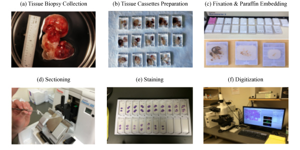
Figure 2.1: Steps involved in the preparation of digital pathology images. Images are borrowed from [62].

2.1 Tissue Preparation

The process of preparing tissue slides for digital pathology analysis begins with a physician requesting a histology confirmation after assessing a patient with a physical exam and/or radiology and laboratory results. The clinical histology process starts by collecting enough good-quality tissue for a diagnosis. There are several approaches for tissue collection, including fine-needle aspiration, needle biopsy, excision biopsy or excision of a lesion in its entirety. Each of these collection techniques can alter the visual analysis of tissues and influence the final diagnosis accuracy. In fact, larger biopsies preserve more cellular context and allow the pathologist to examine multiple slides from different areas of the sampled tissue. Hence, the diagnosis is generally more reliable and accurate when determined from tissues collected with entire lesion excision as opposed to fine-needle aspiration. The sensitivity and specificity of computerized systems to the collection method are not clearly defined yet but one can assume that larger biopsy specimens would allow for a better diagnosis as they would result in more information (more images) but also more preserved context. After biopsy, a pathologist analyses the tissue at a macroscopic scale, measuring it and trimming it to fit into a tissue cassette container of size $10\times 10\times 3$ mm for the subsequent processing steps.

At this stage tissues are transparent, soft and thick and will undergo series of steps allowing for their microscopy visual assessment. First, the collected tissue is immersed into a fixative solution that is used to stop cells from breaking down and tissues to be altered by microorganisms growth. After fixation, most tissues are embedded in a hardening material (i.e., paraffin waxes) to facilitate their sectioning (i.e., cutting) using a microtome. Certain tissues will require quick analysis and are frozen and sectioned in a cryostat (a microtome inside a freezer). Fixation and sectioning are critical steps in the preparation of histopathology slides as they prevent autolysis (i.e., cellular self-destruction by enzymes), allow the tissue to be kept close to its living state without loss of arrangement, and minimize changes in shape or volume often caused by subsequent steps.

Once fixed and sectioned, tissue slices are still nearly invisible under a microscope as biological tissues are transparent. Therefore, another important step in the tissue preparation is tissue staining, which is the process of using dyes (generally chemical agents or antibody agents in the case of immunohistochemical staining) that have affinity for certain cell and extra-cellular components in order to create contrast. The chemical properties of these dyes produce the visual appearance that is seen under the microscope. In both diagnostic and research histopathology, the gold standard tissue sections are stained with hematoxylin and eosin (H&E) where the cell nuclei are stained in blue by the hematoxylin which stains nucleic acids while cell cytoplasm is stained in pink/red by the eosin which stains proteins [20]. Finally, after staining, a coverslip (i.e., small glass sheet) is placed over the tissue mounted on the glass slide. This step creates an even thickness for viewing the tissue under a microscope and prevents the microscope lens from touching the tissue.

While some parts of the tissue preparation procedure can be automated in certain pathology centers (e.g., tissue fixation and sectioning can be done automatically with specific laboratory workstations), tissue handling involves manual intervention and introduces recognizable and well-documented artefacts in the case of paraffin fixed and H&E stained tissue sections but less identifiable artefacts for other dyes. On average, tissue preparation takes 9 to 12 hours [55]. After preparation, tissues can be digitized.

2.2 Tissue Slide Digitization

Whole slide scanners are optical microscopes under robotic and computer control. These microscopes are mounted with highly specialized cameras containing advanced optical sensors that offer spatial resolutions of approximately 0.23-0.25 $\mu$/pixel using the 40x microscope objective [14]. The essential components of a whole slide scanner, generally include the following: 1) a microscope with lens objectives, 2) light source (bright field and/or fluorescent), 3) robotics to load and move tissue slides around, 4) one or more digital cameras for capturing images, 5) a computer, and 6) software to manipulate, manage, and view the digitized slides.

Most whole slide scanners use a tiling or a line-scanning system to produce a WSI. Tiling consists of acquiring multiple individual high-resolution images as tiles while line-scanning creates linear scans of tissue areas. Both systems require stitching and smoothing the tiles or line scans together to create a single digital image of the histologic section.

An important distinction between digital pathology and light microscopy resides in the concepts of magnification and resolution. In digital pathology, these concepts must be considered in the context of how images are acquired and displayed. In fact, magnification in light microscopy is determined by multiplying the power of the objective (4x, 10x, 20x or 40x) by the power of the eyepiece (generally 10x). This concept is not applicable in whole slide imaging as images are viewed on variably sized screens that can further amplify or shrink the original magnification. Hence, in digital pathology, for a whole slide image, the resolution is defined by the objective used to scan the slide (usually referred to as the WSI magnification) and the imaging sensor and is measured in micrometers per pixel.

Once digitized, histopathology tissue sections are stored as WSIs which are digital files with varying sizes. The size of the file depends on the scanning objective and tissue size but commonly ranges from 200 MB to 10GB [98]. In the context of health-care facilities, WSI files are significantly larger than digital image files routinely used in other clinical specialties such as radiology [35]. Therefore, compression-decompression methods, both lossy (e.g., JPEG2000) and loss-less (e.g., TIFF) types, are employed to store WSI. Currently, there is no standard file format for digital pathology images [98], although many vendors use the SVS format which stores a WSI as a multi-layered pyramid of thousands of image files with conserved filed of view and tile size spanning multiple folders. The pyramid representation enable the optimized real-time viewing of a WSI across multiple resolutions. Although, the JPEG2000 compressed format is being used by some vendors there is an interest in migrating to the DICOM format as used in digital radiography [98].

2.3 Artefacts

In pathology, artefacts are the result of the alteration of a tissue from its living state but in digital pathology, artefacts also include alterations of the rendered tissue image.

The preparation of tissue slides and their digitization inevitably results in artefacts of various types that can compromise the image analysis and diagnosis. In fact, tissue appearance can be altered by the fixation, the specimen orientation in the block, the sectioning and the staining or immunolabelling steps which heavily dependent on human skills or, if automated, on human monitoring, machine maintenance and solution preparation [70]. Differences in protocols between pathology labs can greatly alter the appearance of even biologically similar tissue samples. Moreover, the digitization step can also introduce additional artefacts. In fact, depending on the digital scanner, the quality and resolution of the digitized tissue slide can vary significantly.

A challenge in digital pathology is in identifying these artefacts and not confusing them with normal tissue components or pathological changes. In practice, pathologists learn to spot artefacts and depending on the extent of the damage on tissues, some sections often have to be manually discarded. Automatic systems can easily be sensitive to image and tissue artefacts which can cause the automatic image analysis systems to fail. For this reason, different pre-processing methods are generally used and most automatic systems have to account for inter and intra-slide variability. While designing automatic WSI analysis systems that are robust to common artefacts observed in digital pathology is still an open problem, feature learning via deep learning models enabled great progress in this direction. We discuss this further in the next chapter.

Chapter 3   Deep Learning Applications in Digital Pathology

Recent applications of deep learning models in various fields resulted in redefining the state-of-the-art results achieved by earlier machine learning techniques. In digital pathology, deep neural networks, when appropriately trained, have proven capable of yielding diagnostic interpretations with accuracy similar to clinical experts [18].

Prior to the success of deep learning models, traditional machine learning models already proved to be useful in digital pathology. In fact, unlike the simplified algorithms pathologists are trained to use, machine learning models enable learning more complex decision functions. However, these conventional machine learning techniques usually do not directly deal with raw data but heavily rely on the data representations (i.e., hand-crafted features such as color, texture or shape), which require considerable domain expertise and sophisticated engineering. Many works have been proposed with hand-designed features that are often task specific, thus, do not generalize well across tissues and sites. Deep learning models, by leveraging unsupervised or supervised feature learning, do not need heavy specialized applications, hence their quick success in digital pathology. In this chapter, we discuss the different applications of deep learning models for a variety of clinical and non-clinical tasks in digital pathology.

3.1 Computer-aided Diagnosis: Automating Clinical Tasks

A number of image analysis tasks in digital pathology involve the quantification and highlight of morphological features (e.g., cell or mitotic count, nuclei grading, epithelial glands morphology). These tasks invariably require the identification (i.e., localization) of histologic primitives (e.g., cell, nuclei, mitosis, epithelium, cellular membranes, etc.). The presence, extent, size and shape or other morphological appearance of these structures are indicators of the presence or severity of disease. For instance, the size of epithelial glands in prostate cancer tend to reduce with higher Gleason patterns. Another motivation for detecting and segmenting histologic primitives arises from the need for counting of objects, generally cells or nuclei. An example application is the Bloom Richardson grading system which is the most commonly used system for diagnosing invasive breast cancers and comprises three main components: tubule formation, nuclear pleomorphism, and mitotic count. Mitotic count, which refers to the number of dividing cells (i.e., mitoses) visible in H&E tissue slides, is widely acknowledged as a good predictor of tumor aggressiveness. In practice, pathologists define mitotic count as the number of mitotic nuclei identified visually in a fixed number of high power fields (HPFs, 400x magnification). Most of these tasks are time-consuming for the human-eye and can be highly sensitive to the level of expertise as well as the subjectivity of pathologists.

The majority of deep learning models proposed for digital pathology use supervised learning in an attempt to automate the different parts of clinical experts’ visual analysis tasks. Identifying histologic primitives is one area of applications for deep learning models. Another area is in the predictive modelling of outcome (i.e., cancer detection and classification, survival analysis) from WSIs which is the ultimate goal of the visual analysis of tissue slides. Both of these areas of application are motivated by the need for faster, more reliable and objective diagnostics and improved patients outcome.

3.2 Non-clinical Tasks

Another category of applications that leverage deep learning models is the result of computer-aided diagnosis itself. In fact, automatic systems generally require handling dataset-related challenges that are not necessarily critical to pathologists and are not directly involved in clinical tasks. Among such challenges, data harmonization, specifically stain normalization is an important factor that was shown critical in the development of computerized systems. While pathologists are less sensitive to tissue variability induced by staining inconsistencies, automatic systems often fail at generalizing to unseen datasets acquired with different staining protocols and can be highly sensitive to staining variations across tissue slides. Recently, deep models were proposed for staining normalization but also domain adaptation to handle such challenges.

Another application concerns the generation of synthetic images via means of digital staining (transferring stains across images), virtual staining (automatically staining unstained tissues) or generative modelling (creating new images with realistic textures and stains). There are different applications for these techniques that we discuss in the remainder of this report. One direct application of generative learning is data augmentation as a way to overcome the scarcity of available annotated datasets.

Finally, a recent and important application of deep models to digital pathology concerns the design of interpretable computational systems. Interpretability is generally a desirable property for most computer-aided diagnostic systems as it facilitates clinical integration. However, existing systems are not generally optimized or designed for promoting interpretability of their outputs and underlying decision rules. Recently, there have been more attempts at designing interpretable deep models.

Chapter 4   Deep Learning for Analyzing Digital Pathology Images

A wide variety of deep learning models have been proposed for analyzing digitized tissue slides. Given the unique characteristics of WSIs many approaches present ways to process these high dimensional images and leverage their special multi-magnification nature. In this chapter, we discuss strategies to handle data scarcity and class imbalance. Then, we present the most commonly employed neural network architectures and describe the variety of deep learning systems, training strategies and validation procedures that have been proposed for use on WSIs.

4.1 Digital Slide Representation and Datasets

Table 1 shows the different public datasets used in the studies we surveyed as well as their corresponding size. In the works we reviewed the datasets used covered a range of approximately 6 to 600 WSIs. While these are relatively small dataset sizes compared to what is usually necessary for training deep learning models (e.g., thousands or millions of images), a unique particularity of WSIs is their very large dimensions. As describe in section 2.2, WSIs contain millions of pixels which can be leveraged efficiently to increase dataset sizes. Hence, all the works we surveyed in Table LABEL:table:sota used a variant of patch-based techniques to augment the dataset size and train deep learning models. For instance, for the task of detecting nuclei in tissue slides, the datasets created from sampled patches centered at annotated nuclei can contain thousands of positive instances from only dozens of available annotated WSIs. Figure 4.1 shows the sizes in terms of WSIs and their total corresponding annotated patches of the datasets used in different studies grouped per publication year.

In practice, representing WSIs with patches is unavoidable. In fact, with current state-of-the-art computing resources, it is impossible to process a WSI in its entirety without extensively down-sampling the image which would result in loosing most of the discriminative details and morphological features of the underlying tissues.

Although patch-based representations are unavoidable, they do come with important shortcomings. First, patch-based representations imply the loss of global context captured within the multi-magnification levels of the tissue slide. In fact, tissues’ structural organization is generally characterized by the different arrangements of cells and can only be observed at the lowest magnification levels (e.g., 20x or 10x) or with very large scale patches. Different works attempt to encode context when training deep models by using a pyramid representation in which input patches are extracted at different magnification levels (often $20x$ and $40x$) and processed with multi-scale [12] or cascaded [19] deep network architectures.

The second problem often faced when using patch-based representations is class imbalance. In fact, most applications involve datasets with very limited annotated positive samples. For instance, in the task of mitotic detection, only a few nuclei are generally labelled as mitotic, and the ratio of mitotic to non-mitotic nuclei can be up to 1 to 1000 which can arguable be defined as a highly imbalanced dataset. Class imbalance problems can be addressed by designing different patch sampling strategies that maximize the ratio of positives to negatives. One common approach is to densely sample positive patches and perform additional data augmentation with affine and elastic deformations on positive patches only. More sophisticated approaches involve crowdsourcing[12] annotations, employing boosting techniques [27] or relying on active learning [108].

For some tasks such as cancer classification, it can be difficult to collect patch level annotations. In fact, most available dataset for cancer diagnosis are labelled at the slide-level only (i.e., an entire WSI is labelled as cancerous or not but the area of cancer is unknown). In these cases, it can be difficult to identify positive from negative patches. Most works treat patches as independent instances and extrapolate the slide-level label to all sampled patches from a given WSI. While this approach can be efficient, it is fundamentally flawed and results in high false positive patch predictions. A more accurate approach involves formulating classification and segmentation tasks with slide-level annotations only as weakly labelled problems and using machine learning frameworks such as multiple instance learning [46] to train the deep learning models. Other strategies involve designing different aggregation techniques to infer a slide-level prediction from all processed patches at inference time. In this case, a trained model is applied on densely sampled patches from a test WSI in a sliding window fashion and a slide-level prediction score map is obtained. The most successful aggregation strategies involve training secondary machine learning models (e.g., random forest) [18] as classifiers on hand-crafted features (e.g., detected tumor size) extracted from the prediction score map obtained from the patch-level deep model.

Finally, a commonly used strategy for overcoming small dataset sizes (despite the large number of patches that can be extracted from a WSI) is to rely on pre-trained deep learning models. In such case, models are first trained on very large datasets from other domains (e.g., natural scene images) and fine-tuned on the smaller available digital pathology datasets. For instance, it has been shown that convolutional neural network (CNN) architectures trained on natural scene images can generalize relatively well (even without fine-tuning) to a variety of digital pathology tasks [18, 24, 61, 94, 69].

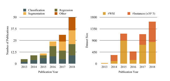
Figure 4.1: Number of studies found per year categorized based on the type of task they address (left) and the average size of the dataset they use (right). The number of instances (#instances) correspond to the average number of annotated instances available.

4.2 Deep Learning Architectures

The majority of deep learning models used in digital pathology are of type feed forward or recurrent neural networks. Neural networks are commonly associated with acyclic graphical models that describe a composition of many different functions $f$ approximating some unknown function $f^{\ast}$. The goal of a neural network is to define a mapping $f(X,\mathcal{W})$ of an input $X$ and learn the parameters $\mathcal{W}$ that result in the best function approximation.

4.2.1 Convolutional Neural Networks

In digital pathology, CNNs are the most commonly used type of feed forward neural networks. A CNN is a composition of a sequence of $L$ layers (i.e., functions) that maps an input image ${\mathbf{X}}$ to an output vector $Y$ (e.g., a scalar or output vector) such that:

$$Y = f({\mathbf{X}};{\mathbf{w}}_{1},{\mathbf{w}}_{2},\dots,{\mathbf{w}}_{L})$$ (4.1)

$$= f_{L}({\mathbf{a}}_{L-1};{\mathbf{w}}_{L})\circ f_{L-1}({\mathbf{a}}_{L-2};{\mathbf{w}}_{L-1})\circ\dots\circ f_{2}({\mathbf{a}}_{1};{\mathbf{w}}_{2})\circ f_{1}({\mathbf{X}};{\mathbf{w}}_{1})$$ (4.2)

where $\mathcal{W}=\{{\mathbf{w}}_{1},{\mathbf{w}}_{2},\dots,{\mathbf{w}}_{L}\}$ are the trainable parameters (weights and biases) at different layers, $\{{\mathbf{a}}_{1},{\mathbf{a}}_{2},\dots,{\mathbf{a}}_{L}\}$ represent the intermediate outputs at each layer that form the networks’ features or internal activations. Conventionally, the successive layers of a CNN model are defined to perform one of the following operations: i) 2D or 3D convolutions with trainable filter banks, ii) spatial pooling (e.g., average or max pooling), iii) non-linear activations (e.g., rectified linear units, hyperbolic tangent, sigmoid). Generally, the final layer of a CNN is represented as a fully connected or dense layer that maps the penultimate output activations to a distribution over categories $P(Y|{\mathbf{X}};\mathcal{W})$ through a softmax function.

Among the works we surveyed in Table LABEL:table:sota, the majority used CNN architectures with relatively shallow architectures (i.e., 2 to 8 layers) when it comes to tasks related to the analysis of histologic primitives (e.g., nuclei and cell localization, cell classification). For instance, many works [36, 41, 69, 61] adopted LeNet [54] and AlexNet [52] architectures with minor modifications to the penultimate layer output size. Both of these networks are relatively shallow, consisting of two and five convolutional layers, respectively and employed convolutional kernels with large receptive fields in early layers and smaller kernels closer to the output. The main distinction of the AlexNet architecture is the use of rectified linear units instead of the hyperbolic tangent as activation function. In contrast, most prediction models we surveyed (e.g., cancer prediction and grading) rely on deeper network architectures (i.e., 8 to 150 layers) [15, 58, 17, 94]. Generally, these architectures are adapted from the VGG-16 [81], Inception [89] and ResNet [42] models which are all built on small fixed-size kernels in each layer. These CNN architectures introduced novel building blocks that were shown to improve training efficiency and reduce the total amount of trainable parameters. Specifically, the Inception model consists of inception blocks where instead of having a single convolution layer applied to a given input, the model uses multiple parallel operations (i.e., convolutions with varying kernel sizes and pooling) applied to the same input. This strategy was shown to act as a multi-level feature extraction scheme. In the ResNet architecture, residual blocks are introduced in order to train very deep models (i.e., 150 layers) effectively. Instead of learning a function, ResNet blocks only learn the residual and are preconditioned towards learning mappings that are close to the identity function. Finally, other works that did not use the above mentioned state-of-the-art architectures [29, 56, 30, 109] designed custom CNN models where the building blocks are typically convolutions with varying kernel sizes depending on the dataset and task, max pooling layers, rectified linear units as activations and fully connected layers that act as final classifier. An example of a common custom architecture is the multi-scale CNN used for mitosis [12] and cell [88] detection. Multi-scale architectures were proposed to incorporate larger context when using patch-based representations of WSIs. A multi-scale CNN is composed of multiple parallel trainable CNN architectures where each network includes a filter bank layer, non-linearity functions and pooling operations and is trained on similar size patches extracted at increasing input image scales. The output predictions obtained for all patches are aggregated using an additional fully connected layer or using a simple geometric average over all prediction scores to predict a single categorical output.

Another application of CNNs in digital pathology is as pixel-level classifiers in segmentation tasks. To predict a class label for each pixel in an input image, a common approach is to use a variant of a CNN named fully convolutional network (FCN) [59]. The particularity of FCNs is that they can receive inputs of arbitrary size and produce correspondingly-sized outputs by removing all fully connected layers and introducing upsampling layers to supplement the usual contracting CNN network composed of stacked convolution, non-linearities and pooling (or downsampling) layers. There are different variants of FCN architectures but the most popular model used in digital pathology is the UNet [77] which uses VGG-16 as a contracting network and combines it with its symmetric counterpart where all pooling layers are replaced by upsampling operations to increase the resolution of the output and form a u-shaped architecture. Skip connections are used to propagate information across the network and facilitate training.

Whether they are used for classification, detection or segmentation, the parameters $\mathcal{W}$ of feed forward neural networks (i.e., CNNs and their variants) are generally trained in a supervised setting by optimizing a cost function. Given a set of $N$ annotated training instances $\{({\mathbf{X}}^{(i)},Y^{(i)})\}$, the parameters $\mathcal{W}$ can be estimated by solving the following optimization problem:

$$\min\limits_{\mathcal{W}}\sum\limits_{i=1}^{N}{\cal L}(P(Y^{(i)}|{\mathbf{X}}^{(i)};\mathcal{W}),Y^{(i)})+{\cal R}(\mathcal{W}),$$ (4.3)

where ${\cal L}$ is a defined cost function and ${\cal R}$ is a regularization term over the trainable parameters $\mathcal{W}$. In most cases, weight decay is used as regularization and the cost function is defined as the cross-entropy loss between the training data and the model’s predictions:

$${\cal L}=-\log\Big{[}P(Y^{(i)}|{\mathbf{X}}^{(i)};\mathcal{W})\Big{]}.$$ (4.4)

Common variants of the cross entropy loss in digital pathology involve adding a weighting coefficient to handle class imbalance [100, 77, 83] or introducing additional auxiliary terms [24] in the loss defined in eq.(4.4).

Most deep models are optimized following eq.(4.3) in an end-to-end fashion using stochastic gradient descent. In order to compute the gradients of the cost function (eq.(4.4)) with respect to the network’s parameters, the backpropagation algorithm is used to allow the information from the cost function to flow backward in a recursive fashion.

4.2.2 Recurrent Neural Networks

Another category of neural networks often used in digital pathology are the recurrent neural networks (RNNs) which are generally used to model sequential data where the input and output (as in feed forward neural networks) can be of varying length. In its simplest form, the particularity of an RNN is in the capacity to maintain a latent or hidden state ${\mathbf{h}}$ at a given time $t$ that is the output of a non-linear mapping from its input ${\mathbf{X}}_{t}$ and given the previous state ${\mathbf{h}}_{t-1}$:

$${\mathbf{h}}_{t}=f({\mathbf{h}}_{t-1},{\mathbf{X}}_{t};\mathcal{W}),$$ (4.5)

where $\mathcal{W}$ are the trainable parameters and $f$ is the non-linear mapping function that is repeatedly applied to all input elements of the sequence ${\mathbf{X}}$. For classification, one or more fully connected layers are typically added followed by a softmax to map the sequence to a posterior over the classes.

The training procedure for a RNN is similar to the one described above in eq.(4.3) with the difference being that the total cost function for a given sequence ${\mathbf{X}}$ paired with a sequence $Y$ is simply the sum of the costs over all time steps (i.e., backpropagation through time).

Different variants of RNNs have been proposed. In digital pathology, the most commonly used recurrent models are gated RNNs and long short term memory (LSTM) networks that use additional gates (i.e., trainable non linear functions) to accumulate and forget information over a long duration of time. LSTMs, as opposed to gated RNN, incorporate gated self loops that are conditioned on the current state and context. These self loops are primarily introduced to facilitate training by modelling long-term dependencies and avoiding the gradients to vanish through the successive time steps.

In the works we reviewed, RNNs and LSTMs have been primarily used for segmentation tasks. In these applications, 2D WSIs are modelled as a sequence of patches and dependencies between local patches are modelled using the recurrent architectures. In order to model dependencies in both axis of the image (i.e., rows and columns), most works use 2D versions of the recurrent networks. For instance, Xie et al. [102] proposed a 2D spatial RNN to segment muscle perimysium in digital pathology images where each input image is partitioned into non overlapping patches. In order to process an input image, the image patches are sorted in an acyclic sequence. Sub-hidden states are introduced and defined as a weighted combination of inputs from the 4-connected adjacent patches (left, right, top and bottom) within rows and columns of a grid representing the organization of all patches in the image. Similarly, 2D LSTMs can be used [10] to capture contextual information by processing WSIs as a 2D sequence of non-overlapping neighbouring patches. The input to the 2D LSTM model is represented as a sequence of two multi-dimensional vectors (e.g., feature vectors obtained with a CNN). Each 2D LSTM unit is pair-wise connected to its 4-connected neighbors and is composed of twice the number of gates as exist in 1D LSTM units (i.e., input, output, forget and cell memory gate) to process inputs from neighbouring patches along the columns and rows of the original WSI.

Generally, recurrent models are integrated within CNN models to obtain feature representations of the input images and do not operate directly on raw input images. In digital pathology, most existing recurrent networks are trained with backpropagation and optimized with the cross entropy loss.

4.2.3 Unsupervised Models

A few works used unsupervised models to process digital pathology images. From the works we reviewed, the majority used auto encoders (or a variant) and generative adversarial networks in an unsupervised setting.

Auto encoders (AEs) are feed forward neural networks that are formed of fully connected or convolutional layers with non linear functions used to compute each layer’s activations. Most existing architectures follow the same design choices as the ones used in CNNs. Generally, AEs are composed of a contracting path that reduces the dimensionality of the input to a coarse latent representation and that is followed by an upsampling path that recovers the input. Thus, AEs are trained to reconstruct an input ${\mathbf{X}}$ on the output layer $\hat{{\mathbf{X}}}$ through one or multiple hidden layers ${\mathbf{h}}$. As AEs are used to reconstruct inputs, they are generally trained with the mean squared error which penalizes the reconstructed input $\hat{{\mathbf{X}}}$ for being dissimilar from the input ${\mathbf{X}}$. A sparse autoencoder (SAE) is simply an AE whose training criterion involves a sparsity penalty on the latent representation $h$, in addition to the reconstruction error. Stacked Sparse auto encoders (SSAE) are formed by stacking multiple auto encoder layers on top of each other and forming deeper networks.

In digital pathology, SSAE were used to obtain feature representations while leveraging datasets in an unsupervised setting (i.e., without requiring annotations). This feature learning strategy was shown successful on a variety of applications such as cancer identification [31, 66] and nuclei detection [105].

Recently, another variant of AEs named variational auto encoders (VAE) was employed to generate grayscale histopathology images [90]. VAEs are probabilistic models used as generative models which aim at learning a probability distribution over a given training dataset. To do so, VAEs are trained to maximize the variational lower bound on the log-likelihood of the data. These models are in essence different from general AEs but they do follow the same architectural design with a contracting path (the encoder) and upsampling path (the decoder). So far, there have been only rare applications of VAEs to digital pathology images.

Another form of generative models that was shown useful in digital pathology are the generative adversarial networks (GAN) [39]. The goal is to learn a generator distribution $P_{G}({\mathbf{X}})$ that matches the real data distribution $P_{d}({\mathbf{X}})$. GANs consist of optimizing a minimax game between a generator $G$ and discriminator network $D$. Both of these networks are generally designed as CNNs. $G$ generates samples from the generator distribution $P_{G}({\mathbf{X}})$ by transforming a noise variable $z\sim P_{n}(z)$ into a sample $G(z)$. $D$ aims at distinguishing samples from the true data distribution $P_{d}({\mathbf{X}})$ from generated samples $G(z)$. The optimization involves finding the parameters of both networks $G$ and $D$ using the following expression:

$$\min\limits_{G}\max\limits_{D}V(D,G)=\mathbb{E}_{x\sim P_{d}}\big{[}\log D({\mathbf{X}})\big{]}+\mathbb{E}_{z\sim P_{n}}\big{[}\log(1-D(G(z)))\big{]}$$ (4.6)

Different variants of GANs have been used in digital pathology for tasks such as data augmentation, data harmonization, domain adaptation and staining normalization [80, 44, 16, 65]. We discuss these works further in section 4.5.1.

4.3 Detection and Analysis of Histologic Primitives

As mentioned previously, a critical prerequisite in the diagnosis of tissue sections is the analysis of histologic primitives such as cells, nuclei, lymphocytes, mitotic figures, etc. The detection of these important tissue components provides support for various quantitative analysis tasks including cell and nuclei morphology, such as size, shape, and texture which are biomarkers of abnormalities.

There exist many challenges in the detection of histologic primitives in digital pathology. First, as mentioned in section 2.3, the appearance of tissue slides can exhibit background clutter introduced during image acquisition but there exist also significant variations on nuclei and cell sizes, shapes and intracellular intensity heterogeneity. Finally, cells and nuclei are often clustered into clumps and may overlap partially with one another. Challenges related to anatomical variations and artefacts make the task of detecting cell and nuclei particularly suited for deep learning models that can potentially learn robust feature representations. In this section we describe different deep learning models proposed for the detection of histologic primitives and specifically present supervised techniques with classification, regression and segmentation deep neural networks as well as unsupervised techniques that leverage deep auto encoders.

4.3.1 Classification Models

Many detection problems (i.e. nuclei, cell, mitosis detection) can be formulated as a pixel or patch-wise classification task and characterized by the appearance of objects to be detected. A common strategy for nuclei or cell detection is to train a CNN classifier as a pixel classifier [48, 57, 68, 106] where the network is trained in a supervised setting using patches centered around the object of interest. The trained CNN model is often a two-class classifier and can be applied in a sliding window fashion on WSIs to detect all histologic components of interest and output a probability map, where each pixel value indicates the probability of one pixel being at the center of an object. Therefore, the target objects can be located, in principle, by seeking local maximum in the generated probability map. This is generally followed by non-maxima suppression to improve the detection results. The advantage of using a deep learning model in this case is mainly in leveraging the learned feature representation that, if the training set allows, can be robust to variations such as rotation, staining appearance, etc. This approach is evidently more accurate than previous state-of-the-art hand-crafted features even when using relatively small architectures such as shown by a variety of works that adopted LeNet-5 [54] the 5-layer CNN model  [75, 97] or proposed 3-layer CNN classifiers to detect cells and nuclei [48, 49].

One important limitation of such pixel-wise classification approach lies in their high computational costs. In practice, sliding window CNNs do not scale well to the million pixel WSIs. To overcome this problem, different strategies have been explored. Wang et al. [97] proposed to reduce redundant computations of neighbouring patches by introducing k-sparse convolution kernels, pooling and fully connected layers that are created by inserting zero rows and columns into the original kernels to enlarge the kernel size hence enabling the network to be trained with larger input tiles. The model is trained on $40\times 40$ patches and tested on $551\times 551$ tiles, hence speeding up the total computation time at test time. In an extension to this work [97], the authors also showed how distributed GPU systems could speed up the total training time [94]. Xu et al. showed the applicability of k-sparse kernels to cell detection on lung cancer images [106]. Giusti et al. [37] achieved a three order magnitude speedup compared to standard sliding window by performing convolutions with larger strides.

Another strategy proposed to improve CNN classifiers for detection tasks consists of utilizing domain knowledge about the object to be detected and leveraging the properties of the H&E staining. In fact, when detecting nuclei or mitotic figures, many works [96, 76, 75, 49] observed that leveraging the hematoxylin channel which highlights nuclei in blue/dark purple would give a good estimate of the potential nuclei centers and hence can be leveraged to generate relevant candidate proposals to use along with the CNN for training. Often the hematoxylin image is filtered out by computing the laplacian of Gaussian (LoG) which allows to detect blob like structures then patches are extracted at those areas of detected nuclei to form candidate proposals [75]. The LoG filter response can also be used to improve color decomposition when separating the hematoxylin and eosin channels [49] which was shown to improve nuclei detection. Chen et al. [23] proposed to use a FCN to first quickly retrieve mitosis candidates and output a score map indicating the probability of mitosis candidates. The FCN is followed by a CNN classifier in a cascaded fashion where the CNN receives the retrieved candidates for further classification into mitotic vs non mitotic nuclei. Both networks share convolutional layers and only the last fully connected layers differ resulting in two different outputs. The model is trained with a softmax classification loss and an L2 regularization term. Along the line of works proposing candidate proposals to use prior to detection; Akram et al. [11] propose a two-branch CNN where one branch regresses on bounding box coordinates and the second predicts a classification score describing how likely the detected box is to include a cell. The generated candidate proposals are then used for training further training a cell classification CNN.

Pixel-wise classification can be easily extended to multi-class organ detection using a softmax loss when training the CNN model. Such multi-class CNN can still be trained with randomly sampled patches and applied on densely sampled patches at test time. A similar strategy was used by Cirecan et al. [27] to win the ICPR 2012 mitosis detection challenge where the task was to identify nuclei in mitotic phase within WSIs. While mitosis are normally rare and well-separated, they are very hard to differentiate from non-mitotic nuclei and the ratio of mitotic to non-mitotic nuclei is generally very low in a tissue slide. Hence, training datasets composed of randomly sampled patches generally suffer from high class imbalance. To overcome this problem, different techniques have been proposed. First, the most straightforward approach consists of sampling balanced datasets and using data augmentation strategies to augment the dataset for positive cases by replication as well as additional forms of augmentation based on affine transforms [61]. Another approach is to leverage non-expert annotated datasets and learn from crowds. Albarquouni et al. [12] proposed AggNet, a CNN model for mitosis detection that can directly handle data aggregation in the learning process such that image annotation from non-experts can be leveraged during training. Specifically, AggNet consists of multi-scale CNNs that are first trained with expert annotations and tested on data. The output after this first round of training is sent to crowdsourcers for relabeling the mistaken annotated images. Then, the networks are refined using the collected annotations and used to generate new ground truth labels.

Finally, another category of works leverages unsupervised learning. Xu et al. [105] proposed a SSAE for nuclei detection in breast cancer images. Their model is first trained in an unsupervised setting with a reconstruction loss and a sparsity constraint. Then, a softmax layer is added as penultimate layer and the model is fine-tuned to classify nuclei patches from non-nuclei patches. At inference, a sliding window method is employed to detect all nuclei within the new tissue slides. Song et al. [86] proposed a hybrid deep auto-encoder to extract high level features from input patches and created probability maps that capture the different shape of nuclei using a Gaussian filtering of image patches centered on cells. The auto encoder is trained to reconstruct the input RGB image as well as the corresponding generated probability map. The predicted detected center points of nuclei are obtained by applying the deep auto encoder to unseen patches and using a second model, here a CNN or SSAE, to perform cell classification on the resulting predicted centers. In an extension [85] to this first work, the classification CNN and the SSAE were coupled to create a model that first detects then classifies cells in WSIs. The coupling is done by adding two branches to the auto encoder: one classifies the detected cells and the other predicts probability maps.

4.3.2 Regression Models

Regression models for cell and nuclei detection were proposed to efficiently locate the centroid of objects. In fact, while CNN classification models produce relatively good results on detection tasks, they do not consider the topological domain on which the output detection resides. In regression analysis, given an input and output pair, the task is to estimate a function that represents the relationship between both variables where the output does not only depend on the input but also on a topological domain (e.g. spatial domain, time).

Most works that address the detection of histology primitives with a regression model define a training output as a proximity score map, which indicates the proximity with respect to the centroid of the object of interest. Generally, the proximity score map is defined as a function resulting in high peak values in the vicinity of the center of the object. For instance, Chen et al. [25] defined the proximity score map as:

$$s(l)=\left\{\begin{matrix}0&x\not\in\mathcal{M}\\ e^{-\frac{||l-c||^{2}}{2\sigma^{2}}}&x\in\mathcal{M}\end{matrix}\right.$$ (4.7)

where $l$ is the position of a pixel in the input patch with respect to the closest centroid $c$ of the object of interest (i.e. mitotic nuclei), $\mathcal{M}$ corresponds to a ground truth segmented mask composed of annotated objects and $\sigma$ is a hyperparameter controlling the variance.

The model is trained with a per-pixel regression loss that minimizes the L2 norm between the predicted proximity score map and $s(l)$. In the deep regression CNN model, an FCN architecture is proposed with an upsampling layer that is used to predict a proximity score map of similar size as the ground truth map $s(l)$. Xie et al. [101] proposed a similar regression CNN for detecting cells in breast, cervex and neuroendocrine tumor tissues but used a weighted L2 loss formulated such that higher penalties are applied for errors on predicted pixels that are closer to the centroid of the cells.

Sirinukunwattana et al. [83, 84] introduced a new CNN layer designed for spatially constrained regression to detect epithelial tumor nuclei in breast and colon cancer datasets. The CNN predicts probability values that are topologically constrained such that high values are concentrated in the vicinity of the center of nuclei. In the spatially constrained CNN architecture, the two penultimate layers are defined to impose these spatial constraints. Specifically, the second to last layer outputs a parameter vector $\theta(x)$ while the final layer outputs a probability map $\hat{y}$ with highest values at the pixels that are strong candidates for being the centers of tumor nuclei such that:

$$\hat{y}_{j}\propto\left\{\begin{matrix}\bigg{(}\frac{1}{1+\frac{1}{2}||z_{j}-\hat{z}^{0}_{m}||^{2}}\bigg{)}h_{m}&\text{if}\quad\forall m\neq m^{\prime}\quad||z_{j}-\hat{z}^{0}_{m}||^{2}\leq||z_{j}-\hat{z}^{0}_{m^{\prime}}||^{2}\\ 0&\text{otherwise}\end{matrix}\right.$$ (4.8)

where $z^{0}_{m}$ represents the coordinates of the center of the $m^{th}$ annotated nucleus within a given patch, $\hat{z}^{0}_{m}$ is the $m^{th}$ estimated nuclei center and $h_{m}\in[0,1]$ is the height of the output probability mask and is a trainable parameter defined as the output of the layer before last. The model is trained with a weighted cross entropy loss that penalizes wrong predictions compared to a pre-computed ground truth regression mask. Finally, to detect the center of nuclei on large test image, the sliding window strategy with overlapping windows is used and the predicted probability of being the center of a nucleus is generated for each of the extracted patches using eq.(4.8). These results are then aggregated to form a probability map where for each pixel location the probability values from all overlapping patches containing the given pixel are averaged. The final detection is obtained from the local maxima found in the probability map. This spatially constrained regression CNN was improved in the work of Kashif et al. [47] where the authors utilized a set of handcrafted features (i.e. color features after color decomposition to isolate hematoxylin channel and texture features based on the scattering transform [60]) as additional inputs to the network and empirically showed sharper prediction results with lower false negative nuclei detection.

To constrain the regression model, Xie et al. [100] proposed a CNN-based approach for nuclei localization that mainly consists of two steps. First, patches extracted from a WSI are assigned a set of voting offset vectors that correspond to a preset number of voting positions, and a corresponding voting confidence score used to weight each vote. Then, the weighted votes are collected for all extracted patches and a final voting density map is computed for the input WSI. The final nuclei positions are identified by the local maxima of the density map.

Generally, detecting cells and nuclei is a first step towards counting or extracting quantitative measures such as nuclei size or total count of cellular structures in a WSI. Another direction for cell/nuclei analysis is to directly predict the desired measurement. Xie et al. [99] proposed to bypass cell detection and directly estimate the total count of cells in histopathology images using a density estimation approach. Specifically, the cell counting problem is cast as a supervised learning problem that tries to learn a mapping from an input image patch to a density map which is a function over pixels in the image that is used to get an estimate of the number of cells in the image after integration. To learn this mapping, the authors proposed a fully convolutional regression network that is trained to regress ground truth density maps from the corresponding input image patches. The model is trained using the mean square error between the predicted heat map and the target density map. At inference, given an input image patch, the model predicts a density map. Two FCN architectures inspired by the VGG-Net architecture adapted with different receptive fields were tested. The authors observed that using larger receptive fields worked best when cells were organized as clumps (where multiple cells overlap) and hence covered larger image patches.

4.3.3 Segmentation Models

Another approach for automating the analysis of histologic primitives is through analyzing the shape and morphology of cells, nuclei, glands or other tissue components. To do so, detection only is not sufficient and a pixel-level delineation of these components is better suited. However, segmentation in digital pathology is often challenging given the high resolution nature of WSI and deep learning models tend to be computationally inefficient on such large images. Most existing deep segmentation models are supervised models that leverage fully convolutional architectures trained with a per-pixel cross entropy loss. In fact, during the 2015 MICCAI Gland Segmentation Challenge [82], the top-5 teams used FCN architectures with different pre and post processing strategies. The challenge winning model [24] was a FCN model with auxiliary layers trained to simultaneously predict a gland boundary mask and a gland mask. Using the auxiliary loss functions as a form of regularization helped training a segmentation model that would converges to more plausible segmentation results in which gland boundaries are not clustered. Such additional domain specific knowledge is often critical when training deep models in digital pathology, especially given the scarcity of the dataset available. We discuss the most representative variants of FCNs in digital pathology below.

Song et al. [88, 87] proposed a multi-scale CNN architecture to segment cervical cytoplasm and nuclei. The WSI is partitioned into patches extracted at multiple scales and a CNN is trained for each scale to classify the central pixel of each patch as nuclei, cytoplasm or background. Feature maps from different scales are then concatenated and a final segmentation mask is obtained using a graph partitioning technique on the extracted features. At inference, the trained multi-scale CNN is applied in a sliding window fashion. Bel et al. [32] also showed the advantage of using a multi-scale CNN model trained with patches extracted at two magnification levels (i.e. 20x and 40x) over a FCN for segmenting nine classes of renal structures. Janowczyk et al. [45] proposed a resolution adaptive deep hierarchical learning framework which uses multiple deep learning networks, with the same architecture, to significantly reduce computation time for fully segmenting high-magnification digital pathology images. Raza et al. [73] also used multiple resolution input patches to train a FCN for segmenting cells in fluorescence images but in contrast to other works, their proposed network uses intermediate layers in the network architecture to enforce better localization and context. The proposed network consists of multiple convolution followed by tanh activation, pooling and upsampling layers. Features from different layers are concatenated to enforce information flow from lower layers of the network to deeper layers. Auxiliary losses are added at different intermediate layers to penalize segmentation errors at cell borders.

Another challenge in segmenting nuclei and cells in WSI is the potential overlap between neighbouring structures which can alter the cell/nuclei shape and boundaries appearance. In order to preserve shapes many works rely on imposing higher order penalties when training segmentation models. While FCNs are generally trained with per-pixel cross entropy loss functions that do not necessarily encode specific shape priors, their output probability maps have been shown useful as unary terms in energy based segmentation models. Xing et al. [103] used such strategy to segment tumor nuclei from overlapping clumps and showed that the probability maps obtained from a trained FCN model formed a robust initialization step for a level set model.

As for detection, segmentation can also be bypassed to directly predict the desired quantification of histologic primitives. For instance, Veta et al. [92] proposed to avoid the nuclei segmentation step and directly predict the nuclear area which is predictive of outcome for breast cancer patients. The authors train a CNN model that is applied locally at each given nucleus location to measure the area of individual nuclei.

4.4 Large tissue analysis and Prediction Models

Often, the purpose of many tasks in digital pathology, such as counting mitoses, quantifying tumour infiltrating immune cells, analyzing the shape of glandular structures of specific tissue entities aim to ultimately predict patient outcome. Therefore, an interesting question is whether these intermediate proxies for outcome could be bypassed and the novel deep learning techniques could be used to directly learn diagnostically relevant features in microscopy images of the tumour, without prior identification of the known tissue entities, e.g., mitoses, nuclear shape, infiltrating immune cells. Different works attempted to train deep learning models using patient outcome as the endpoint to see if such model could reveal known prognostic morphologies, but also has the potential to identify previously unknown prognostic features [17]. We review some of these works in the following section.

4.4.1 Deep Classification and Segmentation Models for Cancer Diagnosis

Given a WSI, automatic cancer diagnosis is generally formulated as assigning a class label to an entire tissue slide (i.e., WSI classification) or identifying abnormal areas of tissues (i.e., WSI segmentation). The majority of existing deep models proposed for predicting the presence of cancer from WSIs use CNNs and FCNs.

There are three main challenges in designing CNN models for cancer prediction from WSIs. All of these challenges arise from the high dimensionality of tissue slides and the limited available annotations for training and validating supervised models. As mentioned in section 4.1, patch-based representations are unavoidable but come with different shortcomings. In this section, we discuss the different strategies proposed for i) training supervised patch-based prediction models using fine-level annotations (i.e., delineations of abnormal tissue areas in a WSI), ii) training weakly supervised patch-based prediction models using only slide-level annotations (i.e., benign vs malignant WSI), iii) encoding the topology of tissues by leveraging the multi-magnification nature of WSIs.

4.4.2 Fully Supervised Models

In fully supervised settings, cancer prediction models can be trained on finely annotated datasets in which one (or several) expert(s) highlighted abnormal areas (e.g., cancerous tissue) within a WSI. In fact, in most applications, only a small portion of the imaged tissue caries morphological and structural patterns indicative of abnormalities. Delineating such areas can be very complex and time consuming as it involves visually identifying abnormal patterns at different magnification levels.

Different works proposed CNN classifiers trained on patches extracted from annotated WSIs to predict the presence of cancer or cancer subtypes. In most works, a fixed magnification level is selected (generally 20x or 40x) and patches are sampled from the set of annotated training WSIs. Sampling strategies in cases where pixel-level annotations are available, involve constructing training mini-batches by randomly selecting samples from points inside and outside the annotated area but within the tissue (i.e., discarding background). For each mini-batch the number of samples per class is generally determined with uniform probabilities [18, 17, 71, 30] and the patch size is often large enough to include structural information (e.g., $224\times 224$). This strategy can work poorly and result in very imbalanced mini-batches in cases where only a fraction of the tissue contains abnormality. This can be the case, for instance, for breast cancer metastasis detection in sentinel lymph nodes where often, only a minuscule fraction of the slide contains cancer and most of the slide is covered by lymphocytes. Also, certain normal regions which look more similar to cancer are typically underrepresented in the training data and patch-based CNN models are generally not capable of correctly identifying these areas as normal. To address this problem, Litjens et al. [56] used a boosting approach to sample training mini-batch patches. This consists of using the initial prediction score maps obtained for the training dataset to sample new patches for both cancerous and non-cancerous classes while increasing the likelihood of sampling patches that were originally incorrectly classified by the model. This process results in additional training data which contains more difficult samples. Subsequently, the model is re-trained using the new sampled patches.

Once the patch-level classification model is trained, it can be used in a sliding window fashion to classify all patches in an unseen WSI and obtain a prediction score map highlighting areas predicted as cancerous. To obtain a slide-level prediction for the entire WSI from the predicted score map, different aggregation techniques have been proposed [58]. Some works simply use the maximum value in the predicted probability score map as the slide-level prediction [104, 58]. One strategy that was shown successful on different datasets [38, 71, 18, 40, 17] consists of leveraging domain knowledge to extract additional hand-crafted features from the predicted score map and train a subsequent classifier to predict a slide-level label. Wang et al. [94] adopted this strategy to win the Cameleyon [18] challenge on identifying metastatic breast cancer from lymph node WSIs. Specifically, 28 geometrical and morphological features were extracted from each predicted score map, including the percentage of tumor region over the whole tissue region, the area ratio between tumor region and the minimum surrounding convex region, the average prediction values, and the longest axis of the tumor region. A random forest classifier is then trained to discriminate WSIs with metastases from the ones without using the hand-crafted features.

4.4.3 Weakly Supervised Models

Weakly supervised models leverage patch-based representation to classify WSIs while only using slide-level annotations during training. Among the works we surveyed, there exist different strategies for training a prediction CNN model using slide-level labels, we present them below.

One commonly used strategy consists of extrapolating the labels from the slide-level to all patches sampled from a given WSI, train a patch-level classifier then use max-voting or pooling to infer the slide-level class. This strategy can be used for patch-level segmentation with FCNs [72] as well as WSI classification [18]. Depending on the complexity of the task and the disparity among patches, this strategy can produce relatively good results. More sophisticated approaches adopt the multiple instance learning framework [46, 43]. For instance, Hou et al. [43] aggregate the prediction of a patch-based CNN model using an Expectation-Maximization (EM) based decision fusion model to automatically locate discriminative patches. In the authors’ formulation, a WSI ${\mathbf{X}}^{(i)}$ is represented as a bag (using the MIL terminology) of instances (i.e., patches) $({\mathbf{x}}^{(i)}_{1},{\mathbf{x}}^{(i)}_{2},\dots,{\mathbf{x}}^{(i)}_{P})$ where $P$ is the total number of instances per bag. Ground truth labels are only available at the bag level. Hidden binary variables $H^{(i)}$ are introduced to model whether an instance of a bag is discriminative or not. Each instance is associated with a hidden variable such that $h^{(i)}_{p}$ represents the hidden variable associated with patch $p$. Assuming all bags and instances are independent, the decision fusion model is defined as follows:

$$P({\mathbf{X}},H)=\prod\limits_{i=1}^{N}\prod_{j=1}^{P}\bigg{(}P({\mathbf{x}}_{j}^{(i)}|h^{(i)}_{j})\bigg{)}P(H^{(i)}),$$ (4.9)

where $N$ is the total number of training WSIs. The likelihood of the data $P({\mathbf{X}})$ is maximized using the EM algorithm and the instance that maximizes $P(h^{(i)}_{j}|{\mathbf{X}}^{(i)})$ is defined as the discriminative instance for the positive bag. Discriminative instances are selected to continue training the CNN prediction model.

Nazeri et al. [67] proposed a two-Stage CNN for classifying breast cancer WSIs. A first CNN, called patch-wise network is trained on patches and outputs spatially smaller feature maps. A second CNN network (named image-wise network) which performs on top of the patch-wise network, receives stacks of feature maps as input and generates slide-level prediction scores. In this cascaded configuration, the second network learns relationships between neighbouring patches represented by their feature maps. The patch-level labels are unknown yet the patch-wise network is trained using the CE loss based on the label of the corresponding WSI. Once trained, the last fully connected layer of the patch-wise network are discarded and only the feature maps obtained from the last convolutional layer are used. The image-wise network is trained on the feature representations obtained from non-overlapping patches using the CE loss again.

Other works proposed to use domain knowledge to identify discriminative patches without requiring patch-level annotations. For instance, Ertosun et al. [34] observed that the grading of gliomas is highly correlated with nuclei morphology, hence, tissue areas with abundant nuclei distribution should be more reflective of the slide-level glioma grade. Based on this observation, the authors trained a CNN model on patches extracted after automatic nuclei detection and showed improved performance against randomly sampled patches.

4.4.4 Encoding Structural Information

Capturing high-level contextual information with patch-based representations is generally difficult as it involves handling larger input image sizes, which does not work well when training deep models. In order to capture context, different works attempt to encode structured relations between neighbouring patches.

One strategy to encode larger context is to employ larger input patches when training the deep prediction models. This strategy was explored by Bejnordi et al. [19] witch stacked multiple CNN models trained sequentially with input patches of increasing size in order to learn fine-gained (cellular) information and global interdependence of tissue structures. The authors leveraged the FCN architecture to train the model with patches of increasing size. Specifically, a first CNN model is trained to classify patches of size $224\times 224$. After convergence, this first model is freezed and converted into a FCN architecture by removing the last fully connected layers. A second network is then stacked on top of the FCN and is similarly trained to classify patches. The input to the second network are the feature maps output of the first FCN. In this cascaded architecture, the second model is trained with input patches with larger size.

Other strategies to encode larger context involve using LSTM units. Agarwalla et al. [10] combined the different feature representations obtained from a patch-level CNN using a 2D LSTM network to encode neighbouring relationships between patches. A 2D-grid of features is generated by packing feature vectors for neighbouring patches in the WSI then four 2D LSTMs running diagonally are used to capture the context information by treating WSIs as a two-dimensional sequence of patches. Finally, tumour predictions across all the spatial dimensions are averaged together to get the final slide-level class label. Similarly, Kong et al. [50] combined CNNs and 2D LSTMs to encode structure between neighboring patches for classifying metastatic tissue slides. The spatial dependencies between patches are explicitly modelled via an additional custom loss function which penalizes the CNN from predicting diverging probability scores for neighbouring patches in a 4-connected neighbourhood.

Finally, Wang et al. [95] attempt to encode structural information related to the contours of microinvasive cervix carcinoma regions in WSIs. Explicitly formulating domain knowledge related to membranes organization is difficult, especially when such information needs to be encoded within a deep learning model. Wang et al.  [95] trained a segmentation FCN model to segment basale membranes of cervix carcinoma tissues. In order to augment the FCN with additional information related to the organization and structure of the membranes’ contours, the authors leverage adversarial training and include a GAN model in which the generator is replaced by the FCN segmentation model and the discriminator learns to identify ground truth membrane contours from predicted segmentation contours.

4.4.5 Survival Prediction Models and Multimodal Applications

Survival analysis is the task of predicting the time duration until an event occurs, which, in digital pathology, corresponds to the death of a patient. In survival datasets, each patient $(i)$ is labelled with a pair $(t^{(i)},\delta^{(i)})$ corresponding to an observation time and a censored status. A censored patient (i.e., patient for which the event is not observed) is characterized by an indicator variable $\delta^{(i)}=0$ while an uncensored patient (i.e., patient for which the event occurred during the study) is characterized by $\delta^{(i)}=1$. The observation time $t^{(i)}$ can be either a survival time $S^{(i)}$ or a censored time $C^{(i)}$ determined by the status indicator variable $\delta^{(i)}$. The most popular survival model is Cox proportional hazard model [28] which is built on the assumption that a patient’s survival risk is a linear combination of covariates (e.g., structured data such as patients’ sex, smoking years, age). However, linear models are not the best suited to model interactions in real-world datasets. This motivated research that leveraged the non-linear deep learning models as survival predictors. We present some of the recent works below.

One way to leverage deep learning models in survival prediction tasks is to employ CNN features to discover new imaging biomarkers. For instance, Yao et al. [109] trained a CNN model to identify cancer from non-cancer cells in tissue patches and used the features from the last convolutional layer of the CNN to extract quantitative descriptors such as textures and geometric properties (e.g., cell area, perimeter, circularity). The extracted features are used to discover imaging biomarkers that correlate with patient survival outcomes using the multivariate cox proportional Hazard model. The authors showed that imaging biomarkers from subtype cell information can better describe tumor morphology and provide more accurate prediction than other techniques relying od molecular profiles. Similarly, Bychkov et al. [22] showed that CNN-derived features extracted from segmented images of epithelium, non-epithelium, and unsegmented tissue micro-array cores correlated well with five-year survival. Bauer et al. [15] showed that a CNN model could be used to classify nuclei in different tissue types (i.e., prostate cancer and renal cell cancer) and that the combination of tissue types during training could increase the overall survival analysis. Zhu et al. [114] showed that the integration of CNN-based features with genomic features into a Cox survival prediction model revealed complementary information on tumor characteristics between pathology images and genetic data.

Other methods employ CNNs to directly predict the survival risk factor. Zhu et al. [113] developed the first deep CNN for survival analysis (DeepConvSurv) with pathological images. The model is trained on patches extracted from tissue areas delineated by experts to regress the survival time for each patch.

$${\cal L}=-\sum\limits_{i\in U}\bigg{(}\beta^{T}a^{(i)}-\log\sum\limits_{j\in\omega^{(i)}}e^{\beta^{T}a^{(j)}}\bigg{)},$$ (4.10)

where $\beta^{T}a^{(i)}$ is the risk associate with the input image with $\beta$ corresponding to the weights of the final fully connected layer and $a^{(i)}$ are its input activations. $U$ and $\omega^{(i)}$ represent the set of right-censored patients (i.e., cases for which the event did not occur at the time of the study) and the set of patients for which the event occurs after $t^{(i)}$.

The authors extended this model to predict survival outcomes for an entire WSI (i.e., a collection of patches) [115]. In this extension, multiple patches are extracted from a given patient’s WSI and clustered based on their phenotype with a k-means clustering approach. Then, clusters are selected based on a their patch-level survival prediction performance using the Cox regression model for predicting survival. The selected clusters are then used to train the DeepConvSurv model described above. All cluster-level survival predictions are then aggregated to obtain a final survival prediction score for an entire WSI.

In practice, patient diagnostic is generally based upon the integration of different sources of information (e.g., omics, radiology, patient history). Consequently, it may be beneficial to integrate these different sources of information into the automatic prediction systems as well. Recent works have attempted to design survival prediction models that integrate both genomic biomarkers and digital pathology images. Yao et al. [110] used a survival CNN model trained on such multi-modal inputs to predict time-to-event outcomes. Their framework showed superior results to the clinicians’ decision rules for predicting the overall survival of patients diagnosed with glioma. Given the current trend in personalized medicine, such multi-modal approaches are becoming more and more critical.

4.5 Non-clinical Tasks

In this section we present categories of work that do not directly attempt to automate clinical tasks but rather focus on facilitating computer-aided diagnosis by improving the quality of input images and datasets to facilitate training or introduce ways to design more interpretable deep learning models.

4.5.1 Stain Normalization, Computational Staining and Augmentation

Stain normalization has always been a critical step in the training of machine learning models. In fact, in contrast to pathologists, most existing machine and deep learning models are sensitive to variations in the staining appearance of tissue slides.

Deep learning models were applied in various ways to normalize stains across datasets. Janowczyk et al. [44] proposed to use features learned with a SAE to normalize stains in different images to a template image. This process was applied by clustering the pixels in a sparse auto-encoded feature space so that respective tissue partitions could be aligned using their respective color distributions. By using individual tissue partitions, this approach is able to more sensitively modify the color space as compared to a global method where all pixels are considered concurrently. GANs have also been employed to normalize stains. Zanjani et al. [111] trained a conditional GAN to generate a colorized H&E image in its CIEL*a*b* space using as input the image lightness channel and a set of structured latent variables drawn randomly from a prior distribution. Finally, Cho et al. [26] defined the problem of stain normalization in the context of domain adaptation and combined it with a prediction task within a GAN framework. The GAN loss described in eq.(4.6) is combined with two additional regularization terms that aim at preventing the degradation of a task-specific network on synthetic images and enforce similar features between synthetic and original images in order to facilitate the task of the generative model.

Conditional GANs were also used in the context of digital staining where the task is to generate images artificially stained with different staining agents. Burlingame et al. [21] used a GAN to convert H&E images to immunofluorescence. Bayramoglu et al. [16] employed a similar conditional GAN to virtually stain unstained hyperspectral specimens.

Finally, GANs have also been employed as data augmentation tools to generate synthetic images. Senaras et al. [80] and Moeskops et al. [65] used a GAN to generate synthetic images and showed that using the synthetized images to augment training datasets increased the performance of prediction and detection models when compared to other standard augmentation strategies.

4.5.2 Interpretability

One recurring critique made against deep learning and machine learning models is their lack of interpretability. Generally, interpretable models in digital pathology are ones for which the output is jutifiable. Deep learning models do not a priori fit in this category and are commonly seen as black-box computational tools. Introducing novel ways to gain insight into the decision making process of deep learning models has become an active area of research in digital pathology.

Cruz-Roa et al. [31] proposed to interpret the predictions of a CNN used to identify cancer in WSIs. Their strategy for interpretability consists of including an interpretable layer that highlights the visual patterns contributing to discriminate between cancerous and normal tissues patterns, working akin to a digital staining which spotlights image regions important for diagnostic decisions. This is achieved by multiplying the feature maps of the trained CNN model by the final layer’s softmax classifier weights. All weighted feature maps are combined into an integrated feature map and a sigmoid function is applied at each pixel of the resulting map. The map is used to highlight areas of the image that were scored as highly discriminative of cancer. While this approach gives a relatively good insight into the trained models’ predictions, it does not really capture the intermediate layers’ contributions to the final outcome.

Korbar et al. [51] proposed a visualization approach to identify discriminative features for colorectal polyps in WSI. In their work, the FCN nature of ResNets is leveraged to directly correlate features with salient areas at each layer. Specifically, the authors used a gradient-based approach to identify discriminative features learned at each intermediate layer of the trained ResNet model. Gradients reflect the change of each intermediate layer function with respect to the input. Hence, visualizing the resulting gradient maps can provide relevant insight on the features distribution per class. However, gradients have generally high variance at intermediate layers and they can be influenced by all different output classes. The authors used a variant of gradient based visualization technique name the class activation map which looks at the change in the penultimate layer’s activations after a single backpropagation pass. A class activation map for a particular class indicates the discriminative image regions used by the CNN to identify that class. The utility of this approach in identifying areas of the input image that justify the most the models’ prediction was tested by comparing the obtained class activation maps with expert annotations. The method showed promising results and relatively good estimates of decisive regions and features for different types of polyps were obtained.

These techniques are a first step toward gaining more insight on the training and output predictions obtained from deep learning models. At a clinical level, interpretability offers a potential avenue for introducing deep learning models into clinical workflows, hence, we can expect future works to continue pursuing this area of research.

4.6 Validation Strategies

A wide variety of metrics have been used to validate the different deep learning models. In the works we reviewed, accuracy, F1 score, precision, recall and area under ROC curve (AUC) were used in majority to evaluate detection and prediction models. Depending on the application, the performance can be reported at the patch or slide-level. Dice scores and FROC are generally used for evaluating segmentation models and measuring the overlap between the predicted segmentation mask and the ground truth annotation. Veta et al. [92] used the Bland-Altman method to evaluate the agreement between two sets of measurements (i.e., predicted vs measured nuclei area). For generative models used in stain normalization tasks, there was no common metric used among the works we surveyed. In fact, some works chose to evaluate the color constancy of the stain normalized images and used the normalized median intensity, others focused on perception-based metrics and reported the accuracy of experts attempting to differentiate synthetic from real images after stain normalization.

To evaluate the performance of prediction models, a few works attempted to compare the performance of the proposed deep learning models with experts on similar test sets. Different metrics have been used to compare humans to machines. For instance, agreement between experts and automatic systems is ideally quantified using the Kappa score. Another approach involves comparing the AUC of an automatic system to the average sensitivity and specificity of different experts. While this is not a completely fair comparison, it gives a relatively good estimate of how far are current systems from becoming part of clinician’s workflow.

With the increase of available public datasets and the emergence of many challenges and competitions, the use of cross-validation techniques to evaluate machine learning systems has reduced. In fact, most released datasets as part of competitions are split into training, validation and test sets and these splits are generally kept fixed to facilitate comparison between the competing methods. This strategy, however, does not allow models to be tested on different training sets.

There exist different types of annotations used in the datasets surveyed in this report. Most datasets were annotated by one (or more) pathologist at the slide or patch level and only a few public datasets provide annotations confirmed by immunohistochemistry, genetics or patient’s outcome. Annotations obtained from experts can be imperfect, especially in tasks such as segmentation of cancer areas where human subjectivity is unavoidable. Also, appropriate use and interpretation of annotations collected from multiple experts remains an open challenge. The gold standard in digital pathology is generally seen as the survival outcome of the patient or their molecular profiling. However, a model that predicts cancer from patient’s survival unavoidably makes strong assumptions regarding the causal relationship between the patient’s observational data (i.e., a digital pathology slide) and their outcome. Verifying the statistical prevalence of such relationship is impossible.

With the increasing number of large dataset collections made publicly available, we can expect evaluation metrics and validation strategies to become more and more standardized.

Chapter 5   Summary and Discussion

Since the adoption of the digital slide for clinical diagnosis there has been a gradual evolution over the years aimed at reducing manual intervention and automating pathologists’ workflow. In the initial phase of digital pathology, traditional computer vision methodologies were used for tissue detection, segmentation, morphometry, and a plethora of other tissue analysis tasks. The main challenges for designing accurate systems are the variability in staining of tissue slides, slide preparation and artefacts resulting from the digitization process.

One particularity of the WSI is its high dimensionality which allowed for early applications of deep learning models with patch-based representations as it provided large enough training sets obtained by sampling patches from the large tissue slide. The studies presented in this survey report the state-of-the-art performance on most WSI analysis tasks (i.e., analysis of histology primitives and outcome prediction) and are all based on (or leverage) patch-based deep learning models. These models have enabled accurate prediction models as well as techniques for identifying and extracting discriminative information from complex tissue images.

While computational imaging with deep learning models can clearly play a role in better quantitative characterization of disease and precision medicine, there still remain a number of substantial technical and computational challenges that need to be overcome before computer assisted image analysis of digital pathology can become part of the routine clinical diagnosis. Although some of the existing deep learning models were designed to overcome challenges related to the WSI size (e.g., patch-based strategies, efficient sampling techniques, faster operations via improved hardware or sparser models), processing the multi-magnification tissue slide without loss of context or structural information remains unsolved. In fact, most of the models employed in the current works are not designed for large input sizes. There is also a need for more standardized and clinically relevant validation protocols as currently none of the existing works were tested on real clinical cohorts. On a similar note, designing automatic cancer diagnosis systems is still an open problem that arises from the lack of available annotated datasets as there is generally no clear clinical consensus on subtyping cancers. Ultimately, the clinical applicability of any deep learning based prediction system will unavoidably result from a collaborative effort between pathologists and computational scientists in order to clearly identify relevant clinical problems and accurately interpret the available annotations.

Aside from improving the performance and interpretability of existing systems, there are many novel directions that could be explored. With the availability of larger datasets such as the TCIA [2] and TCGA [1] data sharing portals, models that can leverage a fusion of modalities (e.g., genomics, histopathology, radiology) for better predictive modelling could be an application area for deep learning. There are also exciting opportunities in leveraging deep models to improve the digital slide acquisition procedure with learning based approaches for signal reconstruction but also flagging systems that can identify altered digital slides (due to staining, fixation or any other artefact caused by the image acquisition) and alleviate the need for manual interventions during the digitization process. On the technical side, the emergence of new datasets such as PCam [7] which is the first dataset for digital pathology that includes more than 300,000 images of size $32\times 32$, brings new opportunities for developing and evaluating customized deep network architectures that are inspired by the challenges proper to tissue images. For instance, one active area of research in this direction is the design of rotation invariant CNN models.

To conclude, by all indications, the digitization of tissue glass slides and the large adoption of deep learning models as computation models is showing significant potential for a transformation of the field of digital pathology from qualitative to quantitative.

Table 5.1: Deep Learning Models for Digital Pathology Applications. The nomenclarture used in this table is as follows. PP:Pre-processing, Augm.:Augmentation, Annot.: annotations, CONV:convolution layer, MP: max pooling, ReLU: rectified linear units, FC: fully connected layer, BN: batch normalization, UP: upsampling, ELU: exponential linear unit, LRN: local response normalization, lReLU: leaky ReLU, ADV: adversarial loss, ConfMat: Confusion matrix, TPV: true predictive value, PPV: positive predictive value. Values separated by ”/” correspond to different datasets used in the corresponding study.

Method	Site	Stain	Mag.	Task	#WSI	#Annot.	Public Data	Input Size	PP	Augm.	Model	#Layers	Ops	Cost	Performance
[27]	Breast	H&E	40x	Mitosis detection	50	300	ICPR2012	$101\times 101$	–	Rotations, Mirroring, Flip	CNN	13	CONV, ReLU, MP, FC	CE	P=0.88, R=0.70, F1=0.78
[61]	Breast	H&E	40x	Mitosis detection	50	300	ICPR2012	$72\times 72$	–	Rotations	LeNet-5	7	CONV, Tanh, MP, FC	CE	F1=0.66
[96]	Breast	H&E	400x	Mitosis detection	50	300	ICPR2012	$80\times 80$	–	Rotations, Mirroring	CNN	3	CONV, ReLU, MP, FC	CE	F1=0.73
[23]	Breast	H&E	40x	Mitosis detection	50	300	ICPR2014	$94\times 94$	–	–	FCN	16		CE	F1=0.79
[12]	Breast	H&E	40x	Mitosis detection	23	–	AMIDA2013	$33\times 33$	–	Rotation, Mirroring,Crowd	CNN	5	CONV, ReLU, MP, FC	CE	AUC=0.86, F1=0.61
[76]	Breast	H&E	40x	Mitosis detection	174		AMIDA	$64\times 64$	–	–	CNN	5	CONV, ReLU, MP, FC, BN	CE	F1=0.56
[75]	Breast	H&E	20x	Tubule detection	174	7513	–	$64\times 64$	–	–	CNN	5	CONV, ReLU, MP, FC	CE	F1=0.59, P=0.72, R=0.56
[48]	Brain Breast	H&E	40x	Nuclei detection	29	13766	–	$51\times 51$	SN	–	CNN	3	CONV, ReLU, MP, FC	CE	P=0.69, R=0.74, F1=0.72
[105]	Breast	H&E	–	Nuclei detection	535	3500	–	$34\times 34$	–	–	SSAE	2	FC	CE	AP=78.83
[49]	Brain Breast	H&E	–	Nuclei detection	29	13766	–	$51\times 51$	–	–	VGG	3	CONV, ReLU, MP, FC, DO	CE	F1=0.84, R=0.81, P=0.88
[11]	Blood Brain Bone Marrow	Fluo	40x	Cell detection	184	–	Fluo-HeLa	$53\times 53$	–	–	FCN	7	CONV, ReLU, MP, FC	CE	IOU=0.72
[97]	Lung	H&E	–	Cell detection	300	–	–	$40\times 40$	–	–	LeNet-5	7	Sparse-CONV, ReLU, MP, FC	CE	F1=0.82
[57]	Lung Neurons	H&E	40x	Cell detection	16/24	150	–	$31\times 31$	–	Rotations	CNN	5	CONV, ReLU, MP, FC	CE	F1=0.90/0.92
[68]	Lung	H&E	–	Cell detection	215	83245	NLST	$20\times 20$	–	–	CNN	7	CONV, ReLU, MP, FC	CE	F1=0.79
[106]	Lung	H&E	40x	Cell detection	215	83245	NLST	$20\times 20$	–	–	LeNet-5	5	CONV, ReLU, MP, FC	CE	F1=0.79
[107]	Lung	H&E	40x	Cell detection	215	83245	–	$20\times 20$	–	–	AE	2	FC	CE	F1=0.83
[86]	Bone Marrow	H&E	–	Cell detection	52	5248	–	$29\times 29$	CD	–	AE	8	FC	CE	P=0.92, R=0.97, F1=0.94
[85]	Bone Marrow	H&E	–	Cell detection	52	5248	–	$29\times 29$	CD	–	AE	2	FC	CE	P=0.92, R=0.97, F1=0.95
[36]	Hep2	IF	–	Cell classification	83	13596	ICPR2014	$78\times 78$	–	Rotation	AlexNet	7	CONV, ReLU, MP, FC, DO	CE	mACC=0.88
[41]	Hep2	IF	–	Cell classif.	83	10000	ICPR2014	$78\times 78$	–	Affine	CNN	5	CONV, ReLU, MP, FC	CE	ACC=0.96
[112]	Blood	H&E	40x	LKC classif.	18	1080	ISBI2012-EM	$11\times 11$	–	None	CNN	4	CONV, MP, FC	CE	ACC=0.93
[63]	MTC	EM	20Kx	MTC classif.	403	403	ICPR2012	$400\times 400$	–	Rotations	LeNet-5	7	CONV, Tanh, SPM, FC	CE	CS=100
[61]	Breast	H&E	40x	Mitotic grade	5	226	AMIDA2013	$72\times 72$	–	None	CNN	10	CONV, ReLU, MP, FC	CE	F1=0.66
[37]	Neuron	EM	–	Neuron segm.	30	–	ISBI2012-EM	$95\times 95$	–	–	CNN	10	CONV, ReLU, MP, FC	CE	Inference time(s)=15.05
[101]	Breast	H&E	40x	Cell detection	32	–	TCGA	$49\times 49$	–	–	CNN	8	CONV, ReLU, MP, FC	WCE	P=0.91, R=0.91, F1=0.91
[100]	Neurones	Ki-67	20x	Nuclei detection	44	–	–	$39\times 39$	–	–	CNN	8	CONV, ReLU, MP, FC, DO	WL2+L1	P=0.85, R=0.79, F1=0.81
[83]	Colon Breast	H&E	20x	Nuclei detection	30		ICPR2014	$27\times 27$	L*ab conversion	Rotation Morroring	CNN	6	CONV, ReLU, MP, FC	WCE	P=0.71/0.73, R=0.85/0.78, F1=0.77/0.75
[84]	Colon	H&E	20x	Nuclei detection	100	20K	CRCHistoNuclei	$27\times 27$	CD	Affine	CNN	8	CONV, ReLU, MP, FC	WCE	P=0.75, R=0.83, F1=0.79
[47]	–	H&E	–	Nuclei detection	15	–	–	$27\times 27$	–	–	CNN	8	CONV, ReLU, MP, FC	CE	P=0.77, R=0.72, F1=0.75
[99]	Blood Retina	H&E	–	Cell counting	2	7000	–	$100\times 100$	–	Synthetic IF images	FCN	7	CONV, ReLU, MP, FC	L2	True/Estimated count=705/696
[25]	Breast	H&E	400x	Mitosis detection	50	300	–	2K$\times$2K	–	–	DeepLab	16	CONV, ReLU, MP, FC	CE	F1=0.79
[92]	Breast	H&E	40x	Nuclei area	39	4264	–	$96\times 96$	–	–	CNN	10	CONV, ReLU, MP, FC	CE	Bland-Altman Bias=-2.98
[88]	Cervex	H&E	40x	Cell segm.	50	8590	–	$32\times 32$	YUV color conversion	Multi-scale	CNN	5	CONV, Tanh, MP, FC	CE	DICE=0.95
[45]	Breast	H&E	40x	Nuclei segm.	137	12K	–	$32\times 32$	–	Multi-scale, Boosting	AlexNet	6	CONV, ReLU, MP, FC, DO	CE	F1=0.82, TPV=0.81, PPV=0.88
[87]	Cervex	H&E	–	Cell segm.	8	20-60	ISBI2015-CELL	$32\times 32$	YUV color conversion	Rotations	CNN	3	CONV, ReLU, MP, FC	CE	DICE=0.89
[103]	Brain Breast	H&E	–	Nuclei segm.	30/35	600K	–	$55\times 55$	YUV color conversion	Rotations	CNN	6	CONV, ReLU, MP, FC	CE	F1=0.77/0.78
[32]	Kidney	H&E	20x	Kidney structures segm.	15	3518	–	$100\times 100$		Elastic	U-Net	22	CONV, ReLU, MP, FC	CE	ConfMat.
[82]	Colon	H&E	40x	Gland segm.	165	–	GLaS	–	SNlization	Elastic	FCN	16	CONV, ReLU, MP, UP	CE	DICE=0.78, Hausdorff=160.3, F1=0.72
[24]	Colon	H&E	40x	Gland segm.	165	–	GLaS	$480\times 480$	–	Affine & elastic	FCN	8	CONV, ReLU, MP, UP	Multi-loss	DICE=0.78, Hausdorff=160.3, F1=0.72
[73]	Pancreas	IF	40x	Cell segm.	–	11K	–	$252\times 252$		Gaussian noise lens distortion flip and rotate	ResNet	50	Residual blocks	WCE	DICE=0.8, ObjectDICE=0.84, Hausdorff=27.5, F1=0.72
[31]	Skin	H&E	10x	Basal Cell Carcinoma detection	1417	–	BCC	$8\times 8$	YUV conversion	–	SSAE		CONV, ReLU,AP,FC	MSE	ACC=0.91
[29]	Breast	H&E	40x	Ivasive Ductal Carcinoma detection	162	–	–	$100\times 100$	–	Bootstrap	CNN	3	CONV, ReLU, MP	CE	ACC=0.84
[56]	Prostate Breast	H&E	–	Cancer detection	254/271	–	–	$128\times 128$	–	–	CNN	6	CONV, ReLU, MP	CE	AUC=0.99/0.88
[30]	Breast	H&E	40x	Cancer detection	584	–	TCGA	$101\times 101$	–	–	CNN	3	CONV, ReLU, MP	CE	DICE=0.76
[18]	Breast	H&E	40x-20x	Metastasis dection	399	–	Camelyon17	$296\times 296$	–	Affine	Inception		Inception blocks	CE	AUC=0.99
[38]	Breast	H&E	–	Metastasis detection	399	–	Camelyon17	$296\times 296$	–	Affine	Inception		Inception blocks	CE	AUC=0.99
[50]	Breast	H&E	40x	Metastasis detection	399	–	Camelyon17	$256\times 256$	–	Affine	ResNet	101	Residual blocks	WCE	FROC=0.75
[15]	Prostate Kidneys	H&E	–	Nuclei classif.	8/6	–	–	–	–	Rotation	Resnet	50	Residual blocks	CE	F1=0.99
[69]	Hep2	IF	–	Cell classif.	28	1457	ICPR2012	$224\times 224$	–	–	AlexNet	8	CONV, ReLU, MP, FC	CE	ACC=0.77
[71]	Breast	IHC	40x	Image scoring	172	–	Her2		–	–	AlexNet Inception	8/16	CONV, ReLU, UP	CE	Agreement Points=382.5
[109]	Lung	H&E	–	Cell classif.	257	–	TCIA-NLST	$40\times 40$	–	–	FCN	3	CONV, ReLU, MP	CE	Kaplan-Meier curves
[104]	Epithelium	IHC H&E	20x	Tissue classif.	157/27	–	Released	$80\times 80$	–	–	FCN	5	CONV, ReLU, MP	CE	ACC=100
[58]	Breast	H&E	40x	Tumor detection and segm.	270	–	Camelyon16	$299\times 299$	–	–	Inception	16	CONV, ReLU, MP	CE	FROC
[67]	Breast	H&E	–	Tissue classif.	400	–	ICIAR18	$512\times 512$	–	Rotations	CNN	15/6	CONV, ReLU, MP	CE	AUC=0.98
[34]	Brain	H&E	20x	Malignant gliomas grading	22	7066	TCGA	$256\times 256$	–	–	CNN	6/12	CONV, ReLU, MP	CE	ConfMat
[66]	Brain Kidney	H&E	40x	Morphometric signatures classif.	2500/ 1400	–	TCGA-KIRC	$100\times 100$	–	Rotation, flip	SAE	2	FC	MSE+L2	ConfMat
[17]	Breast	H&E	20x	Cancer classif.	646	–	–	$224\times 224$	–	Affine	VGG	16	CONV, ReLU, MP,UP	WCE	AUC=0.92
[94]	Breast	H&E	40x	Metastatic cancer detection and classif.	400	–	Camelyon16	$256\times 256$	–	Rotations, flips, crops	GoogleNet	27	CONV, ReLU, MP, BN	CE	AUC=0.93
[40]	lung	H&E	20X	Cancer grading	64	65K	MICCAI-CPM17	$224\times 224$	–	–	ResNet	32	Residual blocks	CE	ACC=0.81
[74]	Prostate	H&E	40x	Gleason grading	270	–	TCGA GDC	$256\times 256$	–	–	CNN LSTM	–	LSTM units	CE	Hazard=206
[43]	Brain lung	H&E	–	Lung cancer classif.	1064	1.1M	TCGA-NSCLC	$500\times 500$	CD	Rotation, mirror, color jitter	CNN	8	CONV, ReLU, MP, LRN, DO	CE	mAP=0.85
[108]	Breast	H&E		Lymph node segm.	85	–	GLaS	–	–	–	FCN	50	Residual blocks	CE	Hausdorff=96.9, DICE=0.86, F1=0.86
[10]	Breast	H&E	40x	Cancer segm.	270	12M	Camelyon16	$224\times 224$	Background removal	–	CNN-LSTM	10	LSTM units	CE	F1=0.83, R=0.83, P=0.81
[95]	Cervix	H&E	40x	Membrane segm.	200	–	–	$500\times 500$	–	Rotations flips	VGG	21	CONV, ReLU, MP, UP	ADV	F1=0.62, P=0.61, R=0.64
[72]	Colon	H&E	20x	Tumor segm.	50	50K	–	$256\times 256$	–	–	CNN	10	CONV, ELU, MP, FC	CE	F1=0.90, P=0.88, R=0.92
[46]	Colon	H&E	–	Cancer segm.	930	–	–	$64\times 64$	–	–	VGG	16	CONV, ReLU, MP, UP	MIL CE	F1=0.83
[22]	Colon	H&E	–	Survival	180	–	–	$585\times 585$	–	–	CNN	9	CONV, ReLU, MP, FC	CE+L2	Hazard=2.08, CI=0.95, AUC=0.66
[15]	Prostate Kidneys	H&E	–	Nuclei classif.	6/8	826/1278	–	$78\times 78$	Grayscale conversion	Affine	ResNet	34	Residual blocks	CE	F1=0.82/0.99
[115]	Lung Brain	H&E	20x	Survival	1104 485 255	67K 70K 60K	NLST/TCIA	$512\times 512$	Background removal	–	CNN	6	CONV, ReLU, MP, FC	Cox regr.	C-index=0.7/0.63/0.60
[113]	Lung	H&E	–	Survival	450	–	NLST	$339\times 339$	–	–	CNN	6	CONV, ReLU, MP, FC	Cox regr.	C-index=0.63
[110]	Lung Brain	H&E Omics	–	Survival	106/126	–	NLST	$1024\times 1024$	–	–	CNN	7	CONV, ReLU, MP, FC	Cox regr.	C-index=0.63/0.64
[64]	Brain	H&E Omics	20x	Survival	769	–	TCGA	$256\times 256$	SN	Mirror, Color jitter	VGG	19	CONV, ReLU, MP, LN, FC	Cox regr.	C-index=0.75
[78]	Breast	H&E	20x	Computational staining	5455	–	TCGA	$100\times 100$	Background removal	Boosting, color jitter	CNN-AE	18	CONV, ReLU, MP, FC	MSE+CE	AUC=0.95
[44]	Breast Colon	H&E	40x	SN	25	200	–	$1000\times 1000$	–	–	SSAE	–	FC	MSE	DICE=0.76
[111]	Breast Liver	H&E	–	SN	125	625	–	$299\times 299$	–	–	InfoGAN	–	–	ADV+R	NMI=0.036
[53]	Breast	H&E	–	Data augm.	238	–	AMIDA2013	$24\times 24$	CD	–	CNN	6	CONV, lReLU, MP, FC	CE	Qualitative
[65]	Breast	H&E	–	Domain adapt.	73	1552	TUPAC	$63\times 63$	–	Color jitter	CNN	6	CONV, ReLU, MP, BN, FC	Multi-loss CE	F1=0.62
[80]	Breast	IHC	40x	Data synthesis	32	–	–	$512\times 512$	–	Color jitter, rotations, flips	cGAN	–	CONV, lReLU, MP, FC	ADV	Experts Fooled ACC=0.47
[16]	Lung	None	40x	Digital staining	–	2838	–	$64\times 64$	PCA	–	cGAN	–	CONV, lReLU, MP, FC	ADV	SSIM=0.39, MSE=2.44
[26]	Breast	H&E	40x	Stain transfer	400	180K	Camelyon16	–	Grayscale conversion	–	cGAN	39	CONV MP FC UP ReLU	ADV+R	AUC=0.91, P=0.84, R=0.85, SP=0.84
[21]	Pancreas	H&E, IF	10x-20x	Digital staining	–	20K	–	$256\times 256$	Registration	Color jitter, rotations, flips	cGAN	–	CONV, ReLU, MP, UP, FC	ADV+R	DICE=0.9, PSNR=31.5, SSIM=0.9
[79]	Lung	H&E	–	Stain transfer	5	–	–	$192\times 192$	–	–	CNN	–	CONV, ReLU, MP, FC	MSE	Qualitative
[90]	Bone marrow	H&E	–	Data synthesis	16	–	Enjoypath	$28\times 28$	Grayscale conversion	–	VAE	–	FC	Lower bound on log-likelihood	NATS=1398.3
[51]	Colon	H&E	–	Feature visualization	176	–	–	$224\times 224$	–	–	ResNet	152	Residual blocks	CE	IOU=0.55

Bibliography

- [1] The cancer genome atlas. https://tcga-data.nci.nih.gov/docs/publications/tcga/.
- [2] The cancer imaging archive. http://www.cancerimagingarchive.net/.
- [3] The cellavision database. http://blog.cellavision.com/.
- [4] The electron microscopy segmentation challenge. http://brainiac2.mit.edu/isbi_challenge/home.
- [5] The enjoypath database. http://www.enjoypath.com/.
- [6] Grand challenge on breast cancer histology images. https://iciar2018-challenge.grand-challenge.org/.
- [7] The pathcamelyon database. https://github.com/basveeling/pcam.
- [8] Tissue micro array analysis in thyroid cancer diagnosis. http://www-o.ntust.edu.tw/~cvmi/ISBI2017/.
- [9] The tumor proliferation assessment challenge. http://tupac.tue-image.nl/.
- [10] Abhinav Agarwalla, Muhammad Shaban, and Nasir M Rajpoot. Representation-aggregation networks for segmentation of multi-gigapixel histology images. arXiv preprint arXiv:1707.08814, 2017.
- [11] Saad Ullah Akram, Juho Kannala, Lauri Eklund, and Janne Heikkilä. Cell segmentation proposal network for microscopy image analysis. In Deep Learning and Data Labeling for Medical Applications, pages 21–29. Springer, 2016.
- [12] Shadi Albarqouni, Christoph Baur, Felix Achilles, Vasileios Belagiannis, Stefanie Demirci, and Nassir Navab. Aggnet: deep learning from crowds for mitosis detection in breast cancer histology images. transactions on medical imaging, 35(5):1313–1321, 2016.
- [13] Ignacio Arganda-Carreras, Srinivas C Turaga, Daniel R Berger, Dan Cireşan, Alessandro Giusti, Luca M Gambardella, Jürgen Schmidhuber, Dmitry Laptev, Sarvesh Dwivedi, Joachim M Buhmann, et al. Crowdsourcing the creation of image segmentation algorithms for connectomics. Frontiers in neuroanatomy, 9:142, 2015.
- [14] Laura Barisoni, Charlotte Gimpel, Renate Kain, Arvydas Laurinavicius, Gloria Bueno, Caihong Zeng, Zhihong Liu, Franz Schaefer, Matthias Kretzler, Lawrence B Holzman, et al. Digital pathology imaging as a novel platform for standardization and globalization of quantitative nephropathology. Clinical kidney journal, 10(2):176–187, 2017.
- [15] Stefan Bauer, Nicolas Carion, Peter Schüffler, Thomas Fuchs, Peter Wild, and Joachim M Buhmann. Multi-organ cancer classification and survival analysis. arXiv preprint arXiv:1606.00897, 2016.
- [16] Neslihan Bayramoglu, Mika Kaakinen, Lauri Eklund, and Janne Heikkila. Towards virtual h&e staining of hyperspectral lung histology images using conditional generative adversarial networks. In Proceedings of the IEEE Conference on Computer Vision and Pattern Recognition, pages 64–71, 2017.
- [17] Babak Ehteshami Bejnordi, Jimmy Lin, Ben Glass, Maeve Mullooly, Gretchen L Gierach, Mark E Sherman, Nico Karssemeijer, Jeroen Van Der Laak, and Andrew H Beck. Deep learning-based assessment of tumor-associated stroma for diagnosing breast cancer in histopathology images. In Biomedical Imaging, 14th International Symposium on, pages 929–932. IEEE, 2017.
- [18] Babak Ehteshami Bejnordi, Mitko Veta, Paul Johannes van Diest, Bram van Ginneken, Nico Karssemeijer, Geert Litjens, Jeroen AWM van der Laak, Meyke Hermsen, Quirine F Manson, Maschenka Balkenhol, et al. Diagnostic assessment of deep learning algorithms for detection of lymph node metastases in women with breast cancer. Jama, 318(22):2199–2210, 2017.
- [19] Babak Ehteshami Bejnordi, Guido Zuidhof, Maschenka Balkenhol, Meyke Hermsen, Peter Bult, Bram van Ginneken, Nico Karssemeijer, Geert Litjens, and Jeroen van der Laak. Context-aware stacked convolutional neural networks for classification of breast carcinomas in whole-slide histopathology images. Journal of Medical Imaging, 4(4):044504, 2017.
- [20] René J Buesa. Histology safety: now and then. Annals of diagnostic pathology, 11(5):334–339, 2007.
- [21] Erik A Burlingame, Adam Margolin, Joe W Gray, and Young Hwan Chang. Shift: speedy histopathological-to-immunofluorescent translation of whole slide images using conditional generative adversarial networks. In Medical Imaging 2018: Digital Pathology, volume 10581, page 1058105. International Society for Optics and Photonics, 2018.
- [22] Dmitrii Bychkov, Riku Turkki, Caj Haglund, Nina Linder, and Johan Lundin. Deep learning for tissue microarray image-based outcome prediction in patients with colorectal cancer. In Medical Imaging 2016: Digital Pathology, volume 9791, page 979115. International Society for Optics and Photonics, 2016.
- [23] Hao Chen, Qi Dou, Xi Wang, Jing Qin, Pheng-Ann Heng, et al. Mitosis detection in breast cancer histology images via deep cascaded networks. In AAAI, pages 1160–1166, 2016.
- [24] Hao Chen, Xiaojuan Qi, Lequan Yu, Qi Dou, Jing Qin, and Pheng-Ann Heng. Dcan: Deep contour-aware networks for object instance segmentation from histology images. Medical image analysis, 36:135–146, 2017.
- [25] Hao Chen, Xi Wang, and Pheng Ann Heng. Automated mitosis detection with deep regression networks. In Biomedical Imaging (ISBI), 2016 IEEE 13th International Symposium on, pages 1204–1207. IEEE, 2016.
- [26] Hyungjoo Cho, Sungbin Lim, Gunho Choi, and Hyunseok Min. Neural stain-style transfer learning using gan for histopathological images. arXiv preprint arXiv:1710.08543, 2017.
- [27] Dan C Cireşan, Alessandro Giusti, Luca M Gambardella, and Jürgen Schmidhuber. Mitosis detection in breast cancer histology images with deep neural networks. In International Conference on Medical Image Computing and Computer-assisted Intervention, pages 411–418. Springer, 2013.
- [28] David R Cox. Regression models and life-tables. In Breakthroughs in statistics, pages 527–541. Springer, 1992.
- [29] Angel Cruz-Roa, Ajay Basavanhally, Fabio González, Hannah Gilmore, Michael Feldman, Shridar Ganesan, Natalie Shih, John Tomaszewski, and Anant Madabhushi. Automatic detection of invasive ductal carcinoma in whole slide images with convolutional neural networks. In Medical Imaging 2014: Digital Pathology, volume 9041, page 904103. International Society for Optics and Photonics, 2014.
- [30] Angel Cruz-Roa, Hannah Gilmore, Ajay Basavanhally, Michael Feldman, Shridar Ganesan, Natalie NC Shih, John Tomaszewski, Fabio A González, and Anant Madabhushi. Accurate and reproducible invasive breast cancer detection in whole-slide images: A deep learning approach for quantifying tumor extent. Scientific reports, 7:46450, 2017.
- [31] Angel Alfonso Cruz-Roa, John Edison Arevalo Ovalle, Anant Madabhushi, and Fabio Augusto González Osorio. A deep learning architecture for image representation, visual interpretability and automated basal-cell carcinoma cancer detection. In International Conference on Medical Image Computing and Computer-Assisted Intervention, pages 403–410. Springer, 2013.
- [32] Thomas de Bel, Meyke Hermsen, Bart Smeets, Luuk Hilbrands, Jeroen van der Laak, and Geert Litjens. Automatic segmentation of histopathological slides of renal tissue using deep learning. In Medical Imaging 2018: Digital Pathology, volume 10581, page 1058112. International Society for Optics and Photonics, 2018.
- [33] Ugljesa Djuric, Gelareh Zadeh, Kenneth Aldape, and Phedias Diamandis. Precision histology: how deep learning is poised to revitalize histomorphology for personalized cancer care. npj Precision Oncology, 1(1):22, 2017.
- [34] Mehmet Günhan Ertosun and Daniel L Rubin. Automated grading of gliomas using deep learning in digital pathology images: A modular approach with ensemble of convolutional neural networks. In AMIA Annual Symposium Proceedings, volume 2015, page 1899. American Medical Informatics Association, 2015.
- [35] Navid Farahani, Anil V Parwani, and Liron Pantanowitz. Whole slide imaging in pathology: advantages, limitations, and emerging perspectives. Pathol Lab Med Int, 7:23–33, 2015.
- [36] Zhimin Gao, Lei Wang, Luping Zhou, and Jianjia Zhang. Hep-2 cell image classification with deep convolutional neural networks. journal of biomedical and health informatics, 21(2):416–428, 2017.
- [37] Alessandro Giusti, Dan C Ciresan, Jonathan Masci, Luca M Gambardella, and Jurgen Schmidhuber. Fast image scanning with deep max-pooling convolutional neural networks. In Image Processing (ICIP), 2013 20th IEEE International Conference on, pages 4034–4038. IEEE, 2013.
- [38] Jeffrey Alan Golden. Deep learning algorithms for detection of lymph node metastases from breast cancer: Helping artificial intelligence be seen. Jama, 318(22):2184–2186, 2017.
- [39] Ian Goodfellow, Jean Pouget-Abadie, Mehdi Mirza, Bing Xu, David Warde-Farley, Sherjil Ozair, Aaron Courville, and Yoshua Bengio. Generative adversarial nets. In Advances in neural information processing systems, pages 2672–2680, 2014.
- [40] Simon Graham, Muhammad Shaban, Talha Qaiser, Syed Ali Khurram, and Nasir Rajpoot. Classification of lung cancer histology images using patch-level summary statistics. In Medical Imaging 2018: Digital Pathology, volume 10581, page 1058119. International Society for Optics and Photonics, 2018.
- [41] Xian-Hua Han, Jianmei Lei, and Yen-Wei Chen. Hep-2 cell classification using k-support spatial pooling in deep cnns. In Deep Learning and Data Labeling for Medical Applications, pages 3–11. Springer, 2016.
- [42] Kaiming He, Xiangyu Zhang, Shaoqing Ren, and Jian Sun. Deep residual learning for image recognition. In Proceedings of the IEEE conference on computer vision and pattern recognition, pages 770–778, 2016.
- [43] Le Hou, Dimitris Samaras, Tahsin M Kurc, Yi Gao, James E Davis, and Joel H Saltz. Patch-based convolutional neural network for whole slide tissue image classification. In Proceedings of the IEEE Conference on Computer Vision and Pattern Recognition, pages 2424–2433, 2016.
- [44] Andrew Janowczyk, Ajay Basavanhally, and Anant Madabhushi. Stain normalization using sparse autoencoders (stanosa): Application to digital pathology. Computerized Medical Imaging and Graphics, 57:50–61, 2017.
- [45] Andrew Janowczyk, Scott Doyle, Hannah Gilmore, and Anant Madabhushi. A resolution adaptive deep hierarchical (radhical) learning scheme applied to nuclear segmentation of digital pathology images. Computer Methods in Biomechanics and Biomedical Engineering: Imaging & Visualization, 6(3):270–276, 2018.
- [46] Zhipeng Jia, Xingyi Huang, I Eric, Chao Chang, and Yan Xu. Constrained deep weak supervision for histopathology image segmentation. IEEE transactions on medical imaging, 36(11):2376–2388, 2017.
- [47] Muhammad Nasim Kashif, Shan E Ahmed Raza, Korsuk Sirinukunwattana, Muhammmad Arif, and Nasir Rajpoot. Handcrafted features with convolutional neural networks for detection of tumor cells in histology images. In Biomedical Imaging (ISBI), 13th International Symposium on, pages 1029–1032. IEEE, 2016.
- [48] Mina Khoshdeli, Richard Cong, and Bahram Parvin. Detection of nuclei in h&e stained sections using convolutional neural networks. In Biomedical & Health Informatics (BHI), 2017 IEEE EMBS International Conference on, pages 105–108. IEEE, 2017.
- [49] Mina Khoshdeli and Bahram Parvin. Feature-based representation improves color decomposition and nuclear detection using a convolutional neural network. IEEE Transactions on Biomedical Engineering, 65(3):625–634, 2018.
- [50] Bin Kong, Xin Wang, Zhongyu Li, Qi Song, and Shaoting Zhang. Cancer metastasis detection via spatially structured deep network. In International Conference on Information Processing in Medical Imaging, pages 236–248. Springer, 2017.
- [51] Bruno Korbar, Andrea M Olofson, Allen P Miraflor, Catherine M Nicka, Matthew A Suriawinata, Lorenzo Torresani, Arief A Suriawinata, and Saeed Hassanpour. Looking under the hood: Deep neural network visualization to interpret whole-slide image analysis outcomes for colorectal polyps. In Computer Vision and Pattern Recognition Workshops (CVPRW), 2017 IEEE Conference on, pages 821–827. IEEE, 2017.
- [52] Alex Krizhevsky, Ilya Sutskever, and Geoffrey E Hinton. Imagenet classification with deep convolutional neural networks. In Advances in neural information processing systems, pages 1097–1105, 2012.
- [53] Maxime W Lafarge, Josien PW Pluim, Koen AJ Eppenhof, Pim Moeskops, and Mitko Veta. Inferring a third spatial dimension from 2d histological images. arXiv preprint arXiv:1801.03431, 2018.
- [54] Yann LeCun, Léon Bottou, Yoshua Bengio, and Patrick Haffner. Gradient-based learning applied to document recognition. Proceedings of the IEEE, 86(11):2278–2324, 1998.
- [55] Geert Litjens, Thijs Kooi, Babak Ehteshami Bejnordi, Arnaud Arindra Adiyoso Setio, Francesco Ciompi, Mohsen Ghafoorian, Jeroen AWM van der Laak, Bram van Ginneken, and Clara I Sánchez. A survey on deep learning in medical image analysis. Medical image analysis, 42:60–88, 2017.
- [56] Geert Litjens, Clara I Sánchez, Nadya Timofeeva, Meyke Hermsen, Iris Nagtegaal, Iringo Kovacs, Christina Hulsbergen-Van De Kaa, Peter Bult, Bram Van Ginneken, and Jeroen Van Der Laak. Deep learning as a tool for increased accuracy and efficiency of histopathological diagnosis. Scientific reports, 6:26286, 2016.
- [57] Fujun Liu and Lin Yang. A novel cell detection method using deep convolutional neural network and maximum-weight independent set. In Deep Learning and Convolutional Neural Networks for Medical Image Computing, pages 63–72. Springer, 2017.
- [58] Yun Liu, Krishna Gadepalli, Mohammad Norouzi, George E Dahl, Timo Kohlberger, Aleksey Boyko, Subhashini Venugopalan, Aleksei Timofeev, Philip Q Nelson, Greg S Corrado, et al. Detecting cancer metastases on gigapixel pathology images. arXiv preprint arXiv:1703.02442, 2017.
- [59] Jonathan Long, Evan Shelhamer, and Trevor Darrell. Fully convolutional networks for semantic segmentation. In Proceedings of the IEEE conference on computer vision and pattern recognition, pages 3431–3440, 2015.
- [60] Stéphane Mallat. Group invariant scattering. Communications on Pure and Applied Mathematics, 65(10):1331–1398, 2012.
- [61] Christopher D Malon and Eric Cosatto. Classification of mitotic figures with convolutional neural networks and seeded blob features. Journal of pathology informatics, 4, 2013.
- [62] Michael T McCann, John A Ozolek, Carlos A Castro, Bahram Parvin, and Jelena Kovacevic. Automated histology analysis: Opportunities for signal processing. IEEE Signal Processing Magazine, 32(1):78–87, 2015.
- [63] Manish Mishra, Sabine Schmitt, Lichao Wang, Michael K Strasser, Carsten Marr, Nassir Navab, Hans Zischka, and Tingying Peng. Structure-based assessment of cancerous mitochondria using deep networks. In Biomedical Imaging (ISBI), 13th International Symposium on, pages 545–548. IEEE, 2016.
- [64] Pooya Mobadersany, Safoora Yousefi, Mohamed Amgad, David A Gutman, Jill S Barnholtz-Sloan, José E Velázquez Vega, Daniel J Brat, and Lee AD Cooper. Predicting cancer outcomes from histology and genomics using convolutional networks. Proceedings of the National Academy of Sciences, page 201717139, 2018.
- [65] Pim Moeskops and Mitko Veta. Domain-adversarial neural networks to address the appearance variability of histopathology images. In Deep Learning in Medical Image Analysis and Multimodal Learning for Clinical Decision Support: Third International Workshop, DLMIA 2017, and 7th International Workshop, ML-CDS 2017, Held in Conjunction with MICCAI 2017, Québec City, QC, Canada, September 14, Proceedings, volume 10553, page 83. Springer, 2017.
- [66] Nandita Nayak, Hang Chang, Alexander Borowsky, Paul Spellman, and Bahram Parvin. Classification of tumor histopathology via sparse feature learning. In Biomedical Imaging (ISBI), 2013 IEEE 10th International Symposium on, pages 410–413. IEEE, 2013.
- [67] Kamyar Nazeri, Azad Aminpour, and Mehran Ebrahimi. Two-stage convolutional neural network for breast cancer histology image classification. arXiv preprint arXiv:1803.04054, 2018.
- [68] Hao Pan, Zheng Xu, and Junzhou Huang. An effective approach for robust lung cancer cell detection. In International Workshop on Patch-based Techniques in Medical Imaging, pages 87–94. Springer, 2015.
- [69] Ha Tran Hong Phan, Ashnil Kumar, Jinman Kim, and Dagan Feng. Transfer learning of a convolutional neural network for hep-2 cell image classification. In Biomedical Imaging (ISBI), 13th International Symposium on, pages 1208–1211. IEEE, 2016.
- [70] Jonas Pichat, Juan Eugenio Iglesias, Tarek Yousry, Sébastien Ourselin, and Marc Modat. A survey of methods for 3d histology reconstruction. Medical image analysis, 46:73–105, 2018.
- [71] Talha Qaiser, Abhik Mukherjee, Chaitanya Reddy Pb, Sai D Munugoti, Vamsi Tallam, Tomi Pitkäaho, Taina Lehtimäki, Thomas Naughton, Matt Berseth, Aníbal Pedraza, et al. Her 2 challenge contest: a detailed assessment of automated her 2 scoring algorithms in whole slide images of breast cancer tissues. Histopathology, 72(2):227–238, 2018.
- [72] Talha Qaiser, Yee-Wah Tsang, David Epstein, and Nasir Rajpoot. Tumor segmentation in whole slide images using persistent homology and deep convolutional features. In Annual Conference on Medical Image Understanding and Analysis, pages 320–329. Springer, 2017.
- [73] Shan E Ahmed Raza, Linda Cheung, David Epstein, Stella Pelengaris, Michael Khan, and Nasir M Rajpoot. Mimo-net: A multi-input multi-output convolutional neural network for cell segmentation in fluorescence microscopy images. In Biomedical Imaging (ISBI 2017), 2017 IEEE 14th International Symposium on, pages 337–340. IEEE, 2017.
- [74] Jian Ren, Kubra Karagoz, Michael Gatza, David J Foran, and Xin Qi. Differentiation among prostate cancer patients with gleason score of 7 using histopathology image and genomic data. In Medical Imaging 2018: Imaging Informatics for Healthcare, Research, and Applications, volume 10579, page 1057904. International Society for Optics and Photonics, 2018.
- [75] David Romo-Bucheli, Andrew Janowczyk, Hannah Gilmore, Eduardo Romero, and Anant Madabhushi. Automated tubule nuclei quantification and correlation with oncotype dx risk categories in er+ breast cancer whole slide images. Scientific reports, 6:32706, 2016.
- [76] David Romo-Bucheli, Andrew Janowczyk, Hannah Gilmore, Eduardo Romero, and Anant Madabhushi. A deep learning based strategy for identifying and associating mitotic activity with gene expression derived risk categories in estrogen receptor positive breast cancers. Cytometry Part A, 91(6):566–573, 2017.
- [77] Olaf Ronneberger, Philipp Fischer, and Thomas Brox. U-net: Convolutional networks for biomedical image segmentation. In International Conference on Medical image computing and computer-assisted intervention, pages 234–241. Springer, 2015.
- [78] Joel Saltz, Rajarsi Gupta, Le Hou, Tahsin Kurc, Pankaj Singh, Vu Nguyen, Dimitris Samaras, Kenneth R Shroyer, Tianhao Zhao, Rebecca Batiste, et al. Spatial organization and molecular correlation of tumor-infiltrating lymphocytes using deep learning on pathology images. Cell reports, 23(1):181, 2018.
- [79] J Schüler and D Merhof. Context-based normalization of histological stains using deep convolutional features. In Deep Learning in Medical Image Analysis and Multimodal Learning for Clinical Decision Support: Third International Workshop, DLMIA 2017, and 7th International Workshop, ML-CDS 2017, Held in Conjunction with MICCAI 2017, Québec City, QC, Canada, September 14, Proceedings, volume 10553, page 135. Springer, 2017.
- [80] Caglar Senaras, Berkman Sahiner, Gary Tozbikian, Gerard Lozanski, and Metin N Gurcan. Creating synthetic digital slides using conditional generative adversarial networks: application to ki67 staining. In Medical Imaging 2018: Digital Pathology, volume 10581, page 1058103. International Society for Optics and Photonics, 2018.
- [81] Karen Simonyan and Andrew Zisserman. Very deep convolutional networks for large-scale image recognition. arXiv preprint arXiv:1409.1556, 2014.
- [82] Korsuk Sirinukunwattana, Josien PW Pluim, Hao Chen, Xiaojuan Qi, Pheng-Ann Heng, Yun Bo Guo, Li Yang Wang, Bogdan J Matuszewski, Elia Bruni, Urko Sanchez, et al. Gland segmentation in colon histology images: The glas challenge contest. Medical image analysis, 35:489–502, 2017.
- [83] Korsuk Sirinukunwattana, Shan E Ahmed Raza, Yee-Wah Tsang, David Snead, Ian Cree, and Nasir Rajpoot. A spatially constrained deep learning framework for detection of epithelial tumor nuclei in cancer histology images. In International Workshop on Patch-based Techniques in Medical Imaging, pages 154–162. Springer, 2015.
- [84] Korsuk Sirinukunwattana, Shan E Ahmed Raza, Yee-Wah Tsang, David RJ Snead, Ian A Cree, and Nasir M Rajpoot. Locality sensitive deep learning for detection and classification of nuclei in routine colon cancer histology images. IEEE transactions on medical imaging, 35(5):1196–1206, 2016.
- [85] Tzu-Hsi Song, Victor Sanchez, Hesham EIDaly, and Nasir Rajpoot. Simultaneous cell detection and classification with an asymmetric deep autoencoder in bone marrow histology images. In Annual Conference on Medical Image Understanding and Analysis, pages 829–838. Springer, 2017.
- [86] Tzu-Hsi Song, Victor Sanchez, Hesham EIDaly, and Nasir M Rajpoot. Hybrid deep autoencoder with curvature gaussian for detection of various types of cells in bone marrow trephine biopsy images. In Biomedical Imaging (ISBI 2017), 2017 IEEE 14th International Symposium on, pages 1040–1043. IEEE, 2017.
- [87] Youyi Song, Ee-Leng Tan, Xudong Jiang, Jie-Zhi Cheng, Dong Ni, Siping Chen, Baiying Lei, and Tianfu Wang. Accurate cervical cell segmentation from overlapping clumps in pap smear images. IEEE transactions on medical imaging, 36(1):288–300, 2017.
- [88] Youyi Song, Ling Zhang, Siping Chen, Dong Ni, Baiying Lei, and Tianfu Wang. Accurate segmentation of cervical cytoplasm and nuclei based on multiscale convolutional network and graph partitioning. IEEE Transactions on Biomedical Engineering, 62(10):2421–2433, 2015.
- [89] Christian Szegedy, Vincent Vanhoucke, Sergey Ioffe, Jon Shlens, and Zbigniew Wojna. Rethinking the inception architecture for computer vision. In Proceedings of the IEEE Conference on Computer Vision and Pattern Recognition, pages 2818–2826, 2016.
- [90] Jakub M Tomczak and Max Welling. Improving variational auto-encoders using householder flow. arXiv preprint arXiv:1611.09630, 2016.
- [91] Martin J van den Bent. Interobserver variation of the histopathological diagnosis in clinical trials on glioma: a clinician’s perspective. Acta neuropathologica, 120(3):297–304, 2010.
- [92] Mitko Veta, Paul J Van Diest, and Josien PW Pluim. Cutting out the middleman: measuring nuclear area in histopathology slides without segmentation. In International Conference on Medical Image Computing and Computer-Assisted Intervention, pages 632–639. Springer, 2016.
- [93] Mitko Veta, Paul J Van Diest, Stefan M Willems, Haibo Wang, Anant Madabhushi, Angel Cruz-Roa, Fabio Gonzalez, Anders BL Larsen, Jacob S Vestergaard, Anders B Dahl, et al. Assessment of algorithms for mitosis detection in breast cancer histopathology images. Medical image analysis, 20(1):237–248, 2015.
- [94] Dayong Wang, Aditya Khosla, Rishab Gargeya, Humayun Irshad, and Andrew H Beck. Deep learning for identifying metastatic breast cancer. arXiv preprint arXiv:1606.05718, 2016.
- [95] Du Wang, Chaochen Gu, Kaijie Wu, and Xinping Guan. Adversarial neural networks for basal membrane segmentation of microinvasive cervix carcinoma in histopathology images. In Machine Learning and Cybernetics (ICMLC), 2017 International Conference on, volume 2, pages 385–389. IEEE, 2017.
- [96] Haibo Wang, Angel Cruz Roa, Ajay N Basavanhally, Hannah L Gilmore, Natalie Shih, Mike Feldman, John Tomaszewski, Fabio Gonzalez, and Anant Madabhushi. Mitosis detection in breast cancer pathology images by combining handcrafted and convolutional neural network features. Journal of Medical Imaging, 1(3):034003, 2014.
- [97] Sheng Wang, Jiawen Yao, Zheng Xu, and Junzhou Huang. Subtype cell detection with an accelerated deep convolution neural network. In International Conference on Medical Image Computing and Computer-Assisted Intervention, pages 640–648. Springer, 2016.
- [98] JD Webster and RW Dunstan. Whole-slide imaging and automated image analysis: considerations and opportunities in the practice of pathology. Veterinary pathology, 51(1):211–223, 2014.
- [99] Weidi Xie, J Alison Noble, and Andrew Zisserman. Microscopy cell counting and detection with fully convolutional regression networks. Computer methods in biomechanics and biomedical engineering: Imaging & Visualization, 6(3):283–292, 2018.
- [100] Yuanpu Xie, Xiangfei Kong, Fuyong Xing, Fujun Liu, Hai Su, and Lin Yang. Deep voting: A robust approach toward nucleus localization in microscopy images. In International Conference on Medical Image Computing and Computer-Assisted Intervention, pages 374–382. Springer, 2015.
- [101] Yuanpu Xie, Fuyong Xing, Xiangfei Kong, Hai Su, and Lin Yang. Beyond classification: structured regression for robust cell detection using convolutional neural network. In International Conference on Medical Image Computing and Computer-Assisted Intervention, pages 358–365. Springer, 2015.
- [102] Yuanpu Xie, Zizhao Zhang, Manish Sapkota, and Lin Yang. Spatial clockwork recurrent neural network for muscle perimysium segmentation. In International Conference on Medical Image Computing and Computer-Assisted Intervention, pages 185–193. Springer, 2016.
- [103] Fuyong Xing, Yuanpu Xie, and Lin Yang. An automatic learning-based framework for robust nucleus segmentation. IEEE transactions on medical imaging, 35(2):550–566, 2016.
- [104] Jun Xu, Xiaofei Luo, Guanhao Wang, Hannah Gilmore, and Anant Madabhushi. A deep convolutional neural network for segmenting and classifying epithelial and stromal regions in histopathological images. Neurocomputing, 191:214–223, 2016.
- [105] Jun Xu, Lei Xiang, Qingshan Liu, Hannah Gilmore, Jianzhong Wu, Jinghai Tang, and Anant Madabhushi. Stacked sparse autoencoder (ssae) for nuclei detection on breast cancer histopathology images. transactions on medical imaging, 35(1):119–130, 2016.
- [106] Zheng Xu and Junzhou Huang. Efficient lung cancer cell detection with deep convolution neural network. In International Workshop on Patch-based Techniques in Medical Imaging, pages 79–86. Springer, 2015.
- [107] Zheng Xu and Junzhou Huang. Detecting 10,000 cells in one second. In International Conference on Medical Image Computing and Computer-Assisted Intervention, pages 676–684. Springer, 2016.
- [108] Lin Yang, Yizhe Zhang, Jianxu Chen, Siyuan Zhang, and Danny Z Chen. Suggestive annotation: A deep active learning framework for biomedical image segmentation. In International Conference on Medical Image Computing and Computer-Assisted Intervention, pages 399–407. Springer, 2017.
- [109] Jiawen Yao, Sheng Wang, Xinliang Zhu, and Junzhou Huang. Imaging biomarker discovery for lung cancer survival prediction. In International Conference on Medical Image Computing and Computer-Assisted Intervention, pages 649–657. Springer, 2016.
- [110] Jiawen Yao, Xinliang Zhu, Feiyun Zhu, and Junzhou Huang. Deep correlational learning for survival prediction from multi-modality data. In International Conference on Medical Image Computing and Computer-Assisted Intervention, pages 406–414. Springer, 2017.
- [111] F Ghazvinian Zanjani, S Zinger, BE Bejnordi, JAWM van der Laak, et al. Stain normalization of histopathology images using generative adversarial networks. In IEEE International Symposium on Biomedical Imaging (ISBI), 4-7 April 2018, Washington DC. Institute of Electrical and Electronics Engineers (IEEE), 2018.
- [112] Jianwei Zhao, Minshu Zhang, Zhenghua Zhou, Jianjun Chu, and Feilong Cao. Automatic detection and classification of leukocytes using convolutional neural networks. Medical & biological engineering & computing, 55(8):1287–1301, 2017.
- [113] Xinliang Zhu, Jiawen Yao, and Junzhou Huang. Deep convolutional neural network for survival analysis with pathological images. In Bioinformatics and Biomedicine (BIBM), 2016 IEEE International Conference on, pages 544–547. IEEE, 2016.
- [114] Xinliang Zhu, Jiawen Yao, Xin Luo, Guanghua Xiao, Yang Xie, Adi Gazdar, and Junzhou Huang. Lung cancer survival prediction from pathological images and genetic data—an integration study. In Biomedical Imaging (ISBI), 2016 IEEE 13th International Symposium on, pages 1173–1176. IEEE, 2016.
- [115] Xinliang Zhu, Jiawen Yao, Feiyun Zhu, and Junzhou Huang. Wsisa: Making survival prediction from whole slide histopathological images. In IEEE Conference on Computer Vision and Pattern Recognition, pages 7234–7242, 2017.