Sage: Parallel Semi-Asymmetric Graph Algorithms for NVRAMs

Abstract

Non-volatile main memory (NVRAM) technologies provide an attractive set of features for large-scale graph analytics, including byte-addressability, low idle power, and improved memory-density. NVRAM systems today have an order of magnitude more NVRAM than traditional memory (DRAM). NVRAM systems could therefore potentially allow very large graph problems to be solved on a single machine, at a modest cost. However, a significant challenge in achieving high performance is in accounting for the fact that NVRAM writes can be much more expensive than NVRAM reads.

In this paper, we propose an approach to parallel graph analytics using the Parallel Semi-Asymmetric Model (PSAM), in which the graph is stored as a read-only data structure (in NVRAM), and the amount of mutable memory is kept proportional to the number of vertices. Similar to the popular semi-external and semi-streaming models for graph analytics, the PSAM approach assumes that the vertices of the graph fit in a fast read-write memory (DRAM), but the edges do not. In NVRAM systems, our approach eliminates writes to the NVRAM, among other benefits.

To experimentally study this new setting, we develop Sage, a parallel semi-asymmetric graph engine with which we implement provably-efficient (and often work-optimal) PSAM algorithms for over a dozen fundamental graph problems. We experimentally study Sage using a 48-core machine on the largest publicly-available real-world graph (the Hyperlink Web graph with over 3.5 billion vertices and 128 billion edges) equipped with Optane DC Persistent Memory, and show that Sage outperforms the fastest prior systems designed for NVRAM. Importantly, we also show that Sage nearly matches the fastest prior systems running solely in DRAM, by effectively hiding the costs of repeatedly accessing NVRAM versus DRAM.

1 Introduction

Over the past decade, there has been a steady increase in the main-memory sizes of commodity multicore machines, which has led to the development of fast single-machine shared-memory graph algorithms for processing massive graphs with hundreds of billions of edges [37, 72, 85, 87] on a single machine. Single-machine analytics by-and-large outperform their distributed memory counterparts, running up to orders of magnitude faster using much fewer resources [37, 65, 85, 87]. These analytics have become increasingly relevant due to a longterm trend of increasing memory sizes, which continues today in the form of new non-volatile memory technologies that are now emerging on the market (e.g., Intel’s Optane DC Persistent Memory). These devices are significantly cheaper on a per-gigabyte basis, provide an order of magnitude greater memory capacity per DIMM than traditional DRAM, and offer byte-addressability and low idle power, thereby providing a realistic and cost-efficient way to equip a commodity multicore machine with multiple terabytes of non-volatile RAM (NVRAM).

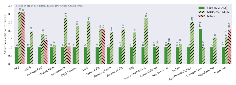
Figure 1: Performance of Sage on the Hyperlink2012 graph compared with existing state-of-the-art systems for processing larger-than-memory graphs using NVRAM measured relative to the fastest system (smaller is better). Sage (NVRAM) are the new codes developed in this paper, GBBS-MemMode is the code developed in [37] run using MemoryMode, and Galois is the NVRAM codes from [43]. The bars are annotated with the parallel running times (in seconds) of the codes on a 48-core system with 2-way hyper-threading. Note that the Hyperlink2012 graph does not fit in DRAM for the machine used in these experiments.

Due to these advantages, NVRAMs are likely to be a key component of many future memory hierarchies, likely in conjunction with a smaller amount of traditional DRAM. However, a challenge of these technologies is to overcome an asymmetry between reads and writes—write operations are more expensive than reads in terms of energy and throughput. This property requires rethinking algorithm design and implementations to minimize the number of writes to NVRAM [10, 15, 16, 27, 98]. As an example of the memory technology and its tradeoffs, in this paper we use a 48-core machine that has 8x as much NVRAM as DRAM (we are aware of machines with 16x as much NVRAM as DRAM [43]), where the combined read throughput for all cores from the NVRAM is about 3x slower than reads from the DRAM, and writes on the NVRAM are a further factor of about 4x slower [50, 96] (a factor of 12 total). Under this asymmetric setting, algorithms performing a large number of writes could see a significant performance penalty if care is not taken to avoid or eliminate writes.

An important property of most graphs used in practice is that they are sparse, but still tend to have many more edges than vertices, often from one to two orders of magnitude more. This is true for almost all social network graphs [57], but also for many graphs that are derived from various simulations [35]. In Figure 2 we show that over 90% of the large graphs (more than 1 million vertices) from the SNAP [57] and LAW [23] datasets have at least 10 times as many edges as vertices. Given that very large graphs today can have over 100 billion edges (requiring around a terabyte of storage), but only a few billion vertices, a popular and reasonable assumption both in theory and in practice is that vertices, but not edges, fit in DRAM [1, 41, 53, 64, 66, 71, 76, 91, 108, 109].

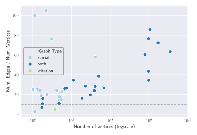
Figure 2: Number of vertices (logscale) vs. average degree $(m/n)$ on 42 real-world graphs with $n>10^{6}$ from the SNAP [57] and LAW [23] datasets. Over 90% of the graphs have average degree larger than 10 (corresponding to the gray dashed line).

With these characteristics of NVRAM and real-world graphs in mind, we propose a semi-asymmetric approach to parallel graph analytics, in which (i) the full graph is stored in NVRAM and is accessed in read-only mode and (ii) the amount of DRAM is proportional to the number of vertices. Although completely avoiding writes to the NVRAM may seem overly restrictive, the approach has the following benefits: (i) algorithms avoid the high cost of NVRAM writes, (ii) the algorithms do not contribute to NVRAM wear-out or wear-leveling overheads, and (iii) algorithm design is independent of the actual cost of NVRAM writes, which has been shown to vary based on access pattern and number of cores [50, 96] and will likely change with innovations in NVRAM technology and controllers. Moreover, it enables an important NUMA optimization in which a copy of the graph is stored on each socket (Section 5), for fast read-only access without any cross-socket coordination. Finally, with no graph mutations, there is no need to re-compress the graph on-the-fly when processing compressed graphs [36, 37].

The key question, then, is the following:

Is the (restrictive) semi-asymmetric approach effective for designing fast graph algorithms?

In this paper, we provide strong theoretical and experimental evidence of the approach’s effectiveness.

Our main contribution is Sage, a parallel semi-asymmetric graph engine with which we implement provably-efficient (and often work-optimal) algorithms for over a dozen fundamental graph problems (see Table 1). The key innovations are in ensuring that the updated state is associated with vertices and not edges, which is particularly challenging (i) for certain edge-based parallel graph traversals and (ii) for algorithms that “delete” edges as they go along in order to avoid revisiting them once they are no longer needed. We provide general techniques (Sections 4.1 and 4.2) to solve these two problems. For the latter, used by four of our algorithms, we require relaxing the prescribed amount of DRAM to be on the order of one bit per edge. Details of our algorithms are given in Section 4.3. Our codes extend the current state-of-the-art DRAM-only codes from GBBS [37], and can be found at https://github.com/ParAlg/gbbs/tree/master/sage.

From a theoretical perspective, we propose a model for analyzing algorithms in the semi-asymmetric setting (Section 3). The model, called the Parallel Semi-Asymmetric Model (PSAM), consists of a shared asymmetric large-memory with unbounded size that can hold the entire graph, and a shared symmetric small-memory with $O(n)$ words of memory, where $n$ is the number of vertices in the graph. In a relaxed version of the model, we allow small-memory size of $O(n+m/\log n)$ words, where $m$ is the number of edges in the graph. Although we do not use writes to the large-memory in our algorithms, the PSAM model permits writes to the large-memory, which are $\omega>1$ times more costly than reads. We prove strong theoretical bounds in terms of PSAM work and depth for all of our parallel algorithms in Sage, as shown in Table 1. Most of the algorithms are work-efficient (performing asymptotically the same work as the best sequential algorithm for the problem) and have polylogarithmic depth (parallel time). These provable guarantees ensure that our algorithms perform reasonably well across graphs with different characteristics, machines with different core counts, and NVRAMs with different read-write asymmetries.

We experimentally study Sage on large-scale real-world graphs (Section 5). We show that Sage scales to the largest publicly-available graph, the Hyperlink2012 graph with over 3.5 billion vertices and 128 billion edges (and 225 billion edges for algorithms running on the undirected/symmetrized graph). Figure 1 compares the performance of Sage algorithms with the fastest available NVRAM approaches on the Hyperlink2012 graph, which is larger than the DRAM of the machine used in our experiments. Compared with the state-of-the-art DRAM codes from GBBS [37], automatically extended to use NVRAM using MemoryMode, Sage is 1.89x faster on average, and slower only in one instance for reasons that we discuss in Section 5. Compared with the recently developed codes from [43], which are the current state-of-the-art NVRAM codes available today, our codes are faster on all five graph problems studied in [43], and achieve an average speedup of 1.94x.

We also study the performance of Sage compared with state-of-the-art graph codes run entirely in DRAM on the largest dataset used in our study that still fits within memory (Figure 7 in Section 5.4). We compare Sage with the GBBS codes run entirely in DRAM, and also when automatically converted to use NVRAM using libvmmalloc, a standard NVRAM memory allocator. Compared with GBBS codes running in DRAM, Sage on NVRAM is only 1.01x slower on average, within 6% of the in-memory running time on all but two problems, and at most 1.82x slower in the worst case. Interestingly, we find that Sage when run in DRAM is 1.17x faster than the GBBS codes run in DRAM on average. This indicates that our optimizations to reduce writes also help on DRAM, although not to the same extent as on NVRAM. In particular, Sage on NVRAM is 6.69x faster on average than GBBS when run on NVRAM using libvmmalloc. Thus, Sage significantly outperforms a naive approach to convert DRAM codes to NVRAM ones, is faster than state-of-the-art DRAM-only codes when run in DRAM, and is highly competitive with the fastest DRAM-only running times when run in NVRAM.

We summarize our contributions below.

1. A semi-asymmetric approach to parallel graph analytics that avoids writing to the NVRAM and uses DRAM proportional to the number of vertices.

2. Sage: a parallel semi-asymmetric graph engine with implementations of 18 fundamental graph problems, and general techniques for semi-asymmetric parallel graph algorithms. We have made all of our codes publicly-available.

3. A new theoretical model called the Parallel Semi-Asymmetric Model, and techniques for designing efficient, and often work-optimal parallel graph algorithms in the model.

4. A comprehensive experimental evaluation of Sage on an NVRAM system showing that Sage significantly outperforms prior work and nearly matches state-of-the-art DRAM-only performance.

2 Preliminaries

Graph Notation. We denote an unweighted graph by $G(V,E)$, where $V$ is the set of vertices and $E$ is the set of edges. The number of vertices is $n=|V|$ and the number of edges is $m=|E|$. Vertices are assumed to be indexed from $0$ to $n-1$. We use $N(v)$ to denote the neighbors of vertex $v$ and $\textit{deg}(v)$ to denote its degree. We focus on undirected graphs in this paper, although many of our algorithms and techniques naturally generalize to directed graphs. We assume that $m=\Omega(n)$ when reporting bounds. We use $\mathsf{d}_{G}$ to refer to the diameter of the graph, which is the longest shortest path distance between any vertex $s$ and any vertex $v$ reachable from $s$. $\Delta$ ($d_{\textit{avg}}$) is used to denote the maximum (average) degree of the graph. We assume that there are no self-edges or duplicate edges in the graph. We refer to graphs stored in the compressed sparse column and compressed sparse row formats as CSC and CSR, respectively. We also consider compressed graphs that store the differences between consecutive neighbors using variable-length codes for each sorted adjacency list [87].

Parallel Cost Model. We use the work-depth model in this paper, and define the model formally when introducing the Parallel Semi-Asymmetric Model model, which extends it (Section 3).

Parallel Primitives. The following parallel procedures are used throughout the paper. Prefix Sum (Scan) takes as input an array $A$ of length $n$, an associative binary operator $\oplus$, and an identity element $\bot$ such that $\bot\oplus x=x$ for any $x$, and returns the array $(\bot,\bot\oplus A[0],\bot\oplus A[0]\oplus A[1],\ldots,\bot\oplus_{i=0}^{n-2}A[i])$ as well as the overall sum, $\bot\oplus_{i=0}^{n-1}A[i]$. Reduce takes an array $A$ and a binary associative function $f$ and returns the sum of the elements in $A$ with respect to $f$. Filter takes an array $A$ and a predicate $f$ and returns a new array containing $a\in A$ for which $f(a)$ is true, in the same order as in $A$. If done in small-memory (Section 3), prefix sum, reduce and filter can all be done in $O(n)$ work and $O(\log n)$ depth (assuming that $\oplus$ and $f$ take $O(1)$ work) [52].

Ligra, Ligra+, and Julienne. As discussed in Section 4, Sage builds on the Ligra [85], Ligra+ [87], and Julienne [36] frameworks for shared-memory graph processing. These frameworks provide primitives for representing subsets of vertices (vertexSubset), and mapping functions over them (edgeMap). edgeMap takes as input a graph $G(V,E)$, a vertexSubset $U\subseteq V$, and two boolean functions $F$ and $C$. edgeMap applies $F$ to $(u,v)\in E$ such that $u\in U$ and $C(v)=\mathit{true}$ (call this subset of undirected edges $E_{a}$), and returns a vertexSubset $U^{\prime}$ where $u\in U^{\prime}$ if and only if $(u,v)\in E_{a}$ and $F(u,v)=\mathit{true}$. $F$ can side-effect data structures associated with the vertices.

3 Parallel Semi-Asymmetric Model

3.1 Model Definition

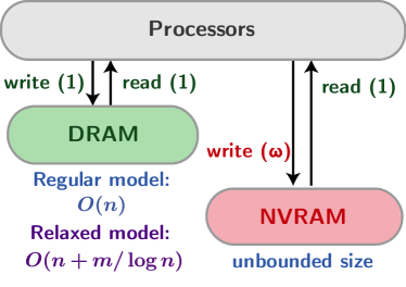
Figure 3: The Parallel Semi-Asymmetric Model. Algorithms in the model perform accesses to a symmetric small-memory (DRAM) and an asymmetric large-memory (NVRAM) at a word-granularity. Reads from both memories are charged unit-cost, whereas writes to the asymmetric memory are charged $\bm{\omega}$. In the regular model, algorithms have access to $O(n)$ words of symmetric memory, and in a relaxed variant have access to $O(n+m/\log n)$ words of symmetric memory. Compared to existing two-level models, the main advantages of the PSAM are that it explicitly models NVRAM read-write asymmetry and it provides sufficient symmetric memory to design provably-efficient and practical parallel graph algorithms.

The Parallel Semi-Asymmetric Model (PSAM) consists of an asymmetric large-memory (NVRAM) with unbounded size, and a symmetric small-memory (DRAM) with $O(n)$ words of memory. In a relaxed version of the model, we allow small-memory size of $O(n+m/\log n)$ words. The relaxed version is intended to model a system where the ratio of NVRAM to DRAM is close to the average degree of real-world graphs (see Figure 2 and Table 2).

The PSAM has a set of threads that share both the large-memory and small-memory. The underlying mechanisms for parallelism are identical to the T-RAM or binary forking model, which is discussed in detail in [13, 18, 37]. In the model, each thread acts like a sequential RAM that also has a fork instruction. When a thread performs a fork, two newly created child threads run starting at the next instruction, and the original thread is suspended until all the children terminate. A computation starts with a single root thread and finishes when that root thread finishes.

Algorithm Cost. We analyze algorithms on the PSAM using the work-depth measure [52]. The work-depth measure is a fundamental tool in analyzing parallel algorithms, e.g., see  [14, 37, 45, 86, 92, 93, 102] for a sample of recent practical uses of this model. Like other multi-level models (e.g., the ANP model [10]), we assume unit cost reads and writes to the small-memory, and reads from the large-memory, all in the unit of a word. A write to the large-memory has a cost of $\omega{}>1$, which is the cost of a write relative to a read on NVRAMs. The overall work $W$ of an algorithm is the sum of the costs for all memory accesses by all threads. The depth $D$ is the cost of the highest cost sequence of dependent instructions in the computation. A work-stealing scheduler can execute a computation in $W/p+O(D)$ time with high probability on $p$ processors [10, 22]. Figure 3 illustrates the PSAM model.

3.2 Discussion

It is helpful to first clarify why we chose to keep the modeling parameters simple, focusing on NVRAM read-write asymmetry, when several other parameters are also available (as discussed below). Our goal was to design a theoretical model that helps guide algorithm design by capturing the most salient features of the new hardware.

Modeling Read and Write Costs. Although NVRAM reads are about 3x more costly than accesses to DRAM [96], we charge both unit cost in the PSAM. When this cost gap needs to be studied (especially for showing lower bounds), we can use an approach similar to the asymmetric RAM (ARAM) model [16], and define the I/O cost $Q$ of an algorithm without charging for instructions or DRAM accesses. All algorithms in this paper have asymptotically as many instructions as NVRAM reads, and therefore have the same I/O cost $Q$ as work $W$ up to constant factors.

Writes to Large-memory. Although in the approach used in this paper we do not perform writes to the large-memory, the PSAM is designed to allow for analyzing alternate approaches that do perform writes to large-memory. Furthermore, permitting writes to the large-memory enables us to consider the cost of algorithms from previous work such as GBBS [37] and observe that many prior algorithms with $W$ work in the standard work-depth model are $\Theta(\omega W)$ work in the PSAM. We emphasize that the objective of this work is to evaluate whether the restrictive approach used in our algorithms—i.e., completely avoiding writes to the large-memory, thereby gaining the benefits discussed in Section 1—is effective compared to existing approaches for programming NVRAM graph algorithms. We note that algorithms designed with a small number of large-memory writes could possibly be quite efficient in practice.

Applicability. In this paper, we provide evidence that the PSAM is broadly applicable for many (18) fundamental graph problems. We believe that many other problems will also fit in the PSAM. For example, counting and enumerating $k$-cliques, which were very recently studied in the in-memory setting [82], can be adapted to the PSAM using the filtering technique proposed in this paper. Other fundamental subgraph problems, such as subgraph matching [47, 94] and frequent subgraph mining [39, 101] could be solved in the PSAM using a similar approach, but mining many large subgraphs may require performing some writes to the NVRAM (as discussed below). Other problems, such as local search problems including CoSimRank [77], personalized PageRank, and other local clustering problems [89], naturally fit in the regular PSAM model.

We note that certain problems seem to require performing writes in the PSAM. For example, in the $k$-truss problem, the output requires emitting the trussness value for each edge, and thus storing the output requires $\Theta(m)$ words of memory, which requires $\Theta(\omega m)$ cost due to writes. Generalizations of $k$-truss, such as the $(r,s)$-nucleii problem appear to have the same requirement for $r\geq 2$ [80].

3.3 Relationship to Other Models

Asymmetric Models. The model considered in this paper is related to the ARAM model [16] and the asymmetric nested-parallel (ANP) model [10]. Compared to these more general models, the PSAM is specially designed for graphs, with its small-memory being either $O(n)$ or $O(n+m/\log n)$ words (for $n$ vertices and $m$ edges).

External and Semi-External Memory Models. The External Memory model (also known as the I/O or disk-access model) [2] is a classic two-level memory model containing a bounded internal memory of size $M$ and an unbounded external memory. I/Os to the external memory are done in blocks of size $B$. The Semi-External Memory model [1] is a relaxation of the External Memory model where there is a small-memory that can hold the vertices but not the edges.

There are three major differences between the PSAM and the External Memory and Semi-External Memory models. First, unlike the PSAM, neither the External Memory nor the Semi-External Memory model account for accessing the small-memory (DRAM), because the objective of these models is to focus on the cost of expensive I/Os to the external memory. We believe that for existing systems with NVRAMs, the cost of DRAM accesses is not negligible. Second, both the External Memory and Semi-External Memory have a parameter $B$ to model data movement in large chunks. NVRAMs support random access, so for the ease of design and analysis we omit this parameter $B$. Third, the PSAM explicitly models the asymmetry of writing to the large memory, whereas the External Memory and Semi-External Memory models treat both reads and writes to the external memory indistinguishably (both cost $B$). The asymmetry of these devices is significant for current devices (writes to NVRAM are 4x slower than reads from NVRAM, and 12x slower than reads from DRAM [50, 96]), and could be even larger in future generations of energy-efficient NVRAMs. Explicitly modeling asymmetry is an important aspect of our approach in the PSAM.

Semi-Streaming Model. In the semi-streaming model [41, 71], there is a memory size of $O(n\cdot\text{polylog}(n))$ bits and algorithms can only read the graph in a sequential streaming order (with possibly multiple passes). In contrast, the PSAM allows random access to the input graph because NVRAMs intrinsically support random access. Furthermore the PSAM allows expensive writes to the large-memory, which is read-only in the semi-streaming model.

4 Sage: A Semi-Asymmetric Graph Engine

Our main approach in Sage is to develop PSAM techniques that perform no writes to the large-memory. Using these primitives lets us derive efficient parallel algorithms (i) whose cost is independent of $\omega$, the asymmetry of the underlying NVRAM technology, (ii) that do not contribute to NVRAM wearout or wear-leveling overheads, and (iii) that do not require on-the-fly recompression for compressed graphs. The surprising result of our experimental study is that this strict discipline—to entirely avoid writes to the large-memory—achieves state-of-the-art results in practice. This discipline also enables storage optimizations (discussed in Section 5), and perhaps most importantly lends itself to designing provably-efficient parallel algorithms that interact with the graph through high-level primitives.

Semi-Asymmetric edgeMap. Our first contribution in Sage is a version of edgeMap (Section 2) that achieves improved efficiency in the PSAM. The issue with the implementation of edgeMap used in Ligra, and subsequent systems (Ligra+ and Julienne) based on Ligra is that although it is work-efficient, it may use significantly more than $O(n)$ space, violating the PSAM model. In this paper, we design an improved implementation of edgeMap which achieves superior performance in the PSAM model (described in Section 4.1). Our result is summarized by the following theorem:

Theorem 4.1

There is a PSAM algorithm for edgeMap given a vertexSubset $U$ that runs in $O(\sum_{u\in U}\textit{deg}(u))$ work, $O(\log n)$ depth, and uses at most $O(n)$ words of memory in the worst case.

Semi-Asymmetric Graph Filtering. An important primitive used by many parallel graph algorithms performs batch-deletions of edges incident to vertices over the course of the algorithm. A batch-deletion operation is just a bulk remove operation that logically deletes these edges from the graph. These deletions are done to reduce the number of edges that must be examined in the future. For example, four of the algorithms studied in this paper—biconnectivity, approximate set cover, triangle counting, and maximal matching—utilize this primitive.

In prior work in the shared-memory setting, deleted edges are handled by actually removing them from the adjacency lists in the graph. In these algorithms, deleting edges is important for two reasons. First, it reduces the amount of work done when edges incident to the vertex are examined again, and second, removing the edges is important to bound the theoretical efficiency of the resulting implementations [36, 37]. In the PSAM, however, deleting edges is expensive because it requires writes to the large-memory.

In our Sage algorithms, instead of directly modifying the underlying graph, we build an auxiliary data structure, which we refer to as a graphFilter, that efficiently supports updating a graph with a sequence of deletions. The graphFilter data structure can be viewed as a bit-packed representation of the original graph that supports mutation. Importantly, this data structure fits into the small-memory of the relaxed version of the PSAM. We formally define our data structure and state our theoretical results in Section 4.2.

Table 1: Work and depth bounds of Sage algorithms in the PSAM. The GBBS Work column shows the work of GBBS algorithms converted to use NVRAM without taking advantage of the small-memory, and corresponds to the GBBS-NVRAM using libvmmalloc experiment (pink dashed-bars in Figure 7). The theoretical performance for the GBBS-MemMode experiment (green dashed-bars in Figure 1) lies in-between the GBBS Work and Sage Work. The vertical text in the first column indicates the technique used to obtain the result in the PSAM: edgeMapChunked is the semi-asymmetric traversal in Section 4.1 and Filter is the Graph Filtering method in Section 4.2. ^† denotes that our algorithm uses $O(n+m/\log n)$ words of memory. ^¶ denotes that our algorithm uses $O(n+m/\log n)$ words of memory in practice, but requires only $O(n)$ words of memory theoretically. ^∗ denotes that a bound holds in expectation and ^‡ denotes that a bound holds with high probability or whp ($O(kf(n))$ cost with probability at least $1-1/n^{k}$). $d_{G}$ is the diameter of the graph, $\Delta$ is the maximum degree, $L=\min{(\sqrt{m},\Delta)}+\log^{2}\Delta\log n/\log\log n$, and $P_{{\scriptsize\mbox{\emph{it}}}}$ is the number of iterations of PageRank until convergence. We assume that $m=\Omega(n)$.

	Problem	GBBS Work	Sage Work	Sage Depth
edgeMapChunked	Breadth-First Search	$O(\omega m)$	$O(m)$	$O(\mathsf{d}_{G}\log n)$
	Weighted BFS	$O(\omega m)^{*}$	$O(m)^{*}$	$O(\mathsf{d}_{G}\log n)$‡
	Bellman-Ford	$O(\omega\mathsf{d}_{G}m)$	$O(\mathsf{d}_{G}m)$	$O(\mathsf{d}_{G}\log n)$
	Single-Source Widest Path	$O(\omega\mathsf{d}_{G}m)$	$O(\mathsf{d}_{G}m)$	$O(\mathsf{d}_{G}\log n)$
	Single-Source Betweenness	$O(\omega m)$	$O(m)$	$O(\mathsf{d}_{G}\log n)$
	$O(k)$-Spanner	$O(\omega m)^{*}$	$O(m)^{*}$	$O(k\log n)$‡
	LDD	$O(\omega m)^{*}$	$O(m)^{*}$	$O(\log^{2}n)$‡
	Connectivity	$O(\omega m)^{*}$	$O(m)^{*}$	$O(\log^{3}n)$‡
	Spanning Forest	$O(\omega m)^{*}$	$O(m)^{*}$	$O(\log^{3}n)$‡
	Graph Coloring	$O(\omega m)^{*}$	$O(m)^{*}$	$O(\log n+L\log\Delta)^{*}$
	Maxmial Independent Set	$O(\omega m)^{*}$	$O(m)^{*}$	$O(\log^{2}n)$‡
Both	Biconnectivity¶	$O(\omega m)^{*}$	$O(m)^{*}$	$O(\mathsf{d}_{G}\log n+\log^{3}n)^{\ddagger}$
	Approximate Set Cover†	$O(\omega m)^{*}$	$O(m)^{*}$	$O(\log^{3}n)$‡
Filter	Triangle Counting†	$O(\omega(m+n)+m^{3/2})$	$O(m^{3/2})$	$O(\log n)$
	Maximal Matching†	$O(\omega m)^{*}$	$O(m)^{*}$	$O(\log^{3}m)$‡
	PageRank Iteration	$O(m+\omega n)$	$O(m)$	$O(\log n)$
	PageRank	$O(P_{\emph{it}}(m+\omega n))$	$O(P_{\emph{it}}m)$	$O(P_{\emph{it}}\log n)$
	$k$-core	$O(\omega m)^{*}$	$O(m)^{*}$	$O(\rho\log n)$‡
	Approximate Densest Subgraph	$O(\omega m)$	$O(m)$	$O(\log^{2}n)$

Efficient Semi-Asymmetric Graph Algorithms. We use our new semi-asymmetric techniques to design efficient semi-asymmetric graph algorithms for 18 fundamental graph problems. In all but a few cases, the bounds are obtained by applying our new semi-asymmetric techniques in conjunction with existing efficient DRAM-only graph algorithms from Dhulipala et al. [37]. We summarize the PSAM work and depth of the new algorithms designed in this paper in Table 1, and present the detailed results in Section 4.3.

4.1 Semi-Asymmetric Graph Traversal

Our first technique is a cache-friendly and memory-efficient sparse edgeMap primitive designed for the PSAM. This technique is useful for obtaining PSAM algorithms for many of the problems studied in this paper. Graph traversals are a basic graph primitive, used throughout many graph algorithms [33, 85]. A graph traversal starts with a frontier (subset) of seed vertices. It then runs a number of iterations, where in each iteration, the edges incident to the current frontier are explored, and vertices in this neighborhood are added to the next frontier based on some user-defined conditions.

4.1.1 Existing Memory-Inefficient Graph Traversal

Ligra implements the direction-optimization proposed by Beamer [8], which runs either a sparse (push-based) or dense (pull-based) traversal, based on the number of edges incident to the current frontier. The sparse traversal processes the out-edges of the current frontier to generate the next frontier. The dense traversal processes the in-edges of all vertices, and checks whether they have a neighbor in the current frontier. Ligra uses a threshold to select a method, which by default is a constant fraction of $m$ to ensure work-efficiency.

The dense method is memory-efficient—theoretically, it only requires $O(n)$ bits to store whether each output vertex is on the next frontier. However, the sparse method can be memory-inefficient because it allocates an array with size proportional to the number of edges incident to the current frontier, which can be up to $O(m)$. In the PSAM, an array of this size can only be allocated in the large-memory, so the traversal is inefficient. This is also true for the real graphs and machines that we tested in this paper.

The GBBS algorithms [37] use a blocked sparse traversal, referred to as edgeMapBlocked, that improves the cache-efficiency of parallel graph traversals by only writing to as many cache lines as the size of the newly generated frontier. This technique is not memory-efficient, as it allocates an intermediate array with size proportional to the number of edges incident to the current frontier, which can be up to $O(m)$ in the worst-case.

4.1.2 Memory-Efficient Traversal: edgeMapChunked

In this paper, we present a chunk-based approach that improves the memory-efficiency of the sparse (push-based) edgeMap. Our approach, which we refer to as edgeMapChunked, achieves the same cache performance as the edgeMapBlocked implementation used in GBBS [37], but significantly improves the intermediate memory usage of the approach. We provide the details of our algorithm and its pseudocode in Appendix A and D.2.

Our Algorithm. The high-level idea of our algorithm is as follows. It first divides the edges that are to-be traversed into grouped units of work. This is done based on the underlying group size, $g$, of the graph, which is set to the average degree $d_{\textit{avg}}$. The edges incident to each vertex are partitioned into groups based on $g$. The algorithm then performs a work-assignment phase, which statically load-balances the work over the incident edges to $O(P)$ virtual threads. Next, in parallel for each virtual thread, it processes the edges assigned to the thread. For each group, it uses a thread-local allocator to obtain a chunk that is ensured to have sufficient memory to store the output of mapping over the edges in the group. The chunks are stored in thread-local vectors. Upon completion of processing all edges incident to the vertexSubset, the algorithm aggregates all chunks stored in the thread-local vectors and uses a prefix-sum and a parallel copy to store the output neighbors contiguously in a single flat array. The overall work of the procedure is $O(\sum_{u\in U}\textit{deg}(u))$ where $U$ is the input vertexSubset, and the depth is $O(\log n)$, which match the work and depth bounds of the previous edgeMapBlocked implementation. We note that for compressed graphs, we must set the underlying group size of the graph to the average degree, which makes the depth $O(\log n+d_{\textit{avg}}{})$ (please see Appendix A for details). Our algorithm also obtains the same cache-efficiency as edgeMapBlocked, while improving the memory usage of the algorithm to $O(n)$ words.

⬇

#include ”sage.h”|\label{line:importsage}|

#include <limits>

template <class W, class Int>|\label{line:bfsstart}|

struct BFSFunc {

sequence<Int>& P;

Int max_int;

BFSFunc(sequence<Int>& P) : P(P) {

max_int = std::numeric_limits<Int>::max();}

bool update(Int s, Int d, W w) {

if (P[d] == max_int) {

P[d] = s;

return 1;

}

return 0;

}

bool updateAtomic(Int s, Int d, W w) {

return (CAS(&P[d], max_int, s));

}

bool cond(Int d) { return (P[d] == max_int); }

}; |\label{line:bfsend}|

template <class Graph, class Int> |\label{line:template}|

sequence<Int> BFS(Graph& G, Int src) {

using W = typename Graph::weight_type;

Int max_int = std::numeric_limits<Int>::max();

auto P = sequence<Int>(G.n, max_int);|\label{line:initparents}|

P[src] = src;|\label{line:setsrcparent}|

auto frontier = vertexSubset(G.n, src); |\label{line:setfrontier}|

while (!frontier.isEmpty()) { |\label{line:whilestart}|

auto F = BFSFunc<W, Int>(P);

frontier = edgeMapChunked(G, frontier, F); |\label{line:emapchunk}|

}|\label{line:whileend}|

return P;

}

Figure 4: Code for Breadth-First Search in Sage.

4.1.3 Case Study: Breadth-First Search

Algorithm. Figure 4 provides the full Sage code used for our implementation of BFS. The algorithm outputs a BFS-tree, but can trivially be modified to output shortest-path distances from the source to all reachable vertices. The user first imports the Sage library (Line LABEL:line:importsage). The definition of BFSFunc defines the user-defined function supplied to edgeMap (Lines LABEL:line:bfsstart–LABEL:line:bfsend). The main algorithm, BFS, is templatized over a graph type (Line LABEL:line:template). The BFS code first initializes the parent array P (Line LABEL:line:initparents), sets the parent of the source vertex to itself (Line LABEL:line:setsrcparent), and initializes the first frontier to contain just the parent (Line LABEL:line:setfrontier). It then loops while the frontier is non-empty (Lines LABEL:line:whilestart–LABEL:line:whileend), and calls edgeMapChunked in each iteration of the while loop (Line LABEL:line:emapchunk).

The function supplied to edgeMapChunked is BFSFunc (Lines LABEL:line:bfsstart–LABEL:line:bfsend), which contains two implementations of update based on whether a sparse or dense traversal is applied (update and updateAtomic respectively), and the function cond indicating whether a neighbor should be visited. This logic is identical to the update function used in BFS in Ligra, and we refer the interested reader to Shun and Blelloch [85] for a detailed explanation.

PSAM: Work-Depth Analysis. The work is calculated as follows. First, the work of initializing the parent array, and constructing the initial frontier is just $O(n)$. The remaining work is to apply edgeMap across all rounds. To bound this quantity, first observe that each vertex, $v$, processes its out-edges at most once, in the round where it is contained in $\mathit{Frontier}$ (if other vertices try to visit $v$ in subsequent rounds notice that the cond function will return false). Let $R$ be the set of all rounds run by the algorithm, $W_{\textsc{edgeMapChunked}{}}(r)$ be the work of edgeMapChunked on the $r$-th round, and $U_{r}$ be the set of vertices in $\mathit{Frontier}$ in the $r$-th round. Then, the work is $\sum_{r\in R}W_{\textsc{edgeMapChunked}{}}(r)=\sum_{r\in R}\sum_{u\in U_{r}}\textit{deg}(u)=O(m)$.

The depth to initialize the parents array is $O(\log n)$, and the depth of each of the $r$ applications of edgeMapChunked is $O(\log n)$ by Theorem 4.1. Thus, the overall depth is $O(r\log n)=O(\mathsf{d}_{G}\log n)$. The small-memory space used for the parent array is $O(n)$ words, and the maximum space used over all edgeMapChunked calls is $O(n)$ words by Theorem 4.1. This proves the following theorem:

Theorem 4.2

There is a PSAM algorithm for breadth-first search that runs in $O(m)$ work, $O(\mathsf{d}_{G}\log n)$ depth, and uses only $O(n)$ words of small-memory.

4.2 Semi-Asymmetric Graph Filtering

Sage provides a high-level filtering interface that captures both the current implementation of filtering in GBBS, as well as the new mutation-avoiding implementation described in this paper. The interface provides functions for creating a new graphFilter, filtering edges from a graph based on a user-defined predicate, and a function similar to edgeMap which filters edges incident to a subset of vertices based on a user-defined predicate. Since edges incident to a vertex can be deleted over the course of the algorithm by using a graphFilter, we call edges that are currently part of the graph represented by the graphFilter as active edges.

We first discuss a semantic issue that arises when filtering graphs. Suppose the user builds a filter $G_{f}$ over a symmetric graph $G$. If the filtering predicate takes into account the directionality of the edge, then the resulting graph filter can become directed, which is unlikely to be what the user intends. Therefore, we designed the constructor to have the user explicitly specify this decision by indicating whether the user-defined predicate is symmetric or asymmetric, which results in either a symmetric or asymmetric graph filter.

The filtering interface is defined as follows:

• makeFilter($G:\mathsf{Graph}$,
                   $P:\mathsf{edge}\mapsto\mathsf{bool}$, $S$ : $\mathsf{bool}$) : $\mathsf{graphFilter{}}$
  Creates a graphFilter $G_{f}$ for the immutable graph $G$ with respect to the user-defined predicate $P$, and $S$, which indicates whether the filter is symmetric or asymmetric.

• filterEdges($G_{f}:\mathsf{graphFilter{}}$) : $\mathsf{int}$
  Filters all active edges in $G_{f}$ that do not satisfy the predicate $P$ from $G_{f}$. The function mutates the supplied graphFilter, and returns the number of edges remaining in the graphFilter.

• edgeMapPack($G_{f}:\mathsf{graphFilter{}}$,
                       $S:\mathsf{vertexSubset{}}):\mathsf{vertexSubset{}}$
  Filters edges incident to $v\in S$ that do not satisfy the predicate $P$ from $G_{f}$. Returns a vertexSubset on the same vertex set as $S$, where each vertex is augmented with its new degree in $G_{f}$.

4.2.1 Graph Filter Data Structure

For simplicity, we describe the symmetric version of the graph filter data structure. The asymmetric filter follows naturally by using two copies of the data structure described below, one for the in-edges and one for the out-edges.

We first review how edges are represented in Sage. In the (uncompressed) CSR format, the neighbors of a vertex are stored contiguously in an array. If the graph is compressed using one of the parallel compression methods from Ligra+ [87], the incident edges are divided into a number of compression blocks, where each block is sequentially encoded using a difference-encoding scheme with variable-length codes. Each block must be sequentially decoded to retrieve the neighbor IDs within the block, but by choosing an appropriate block size, the edges incident to a high-degree vertex can be traversed in parallel across the blocks.

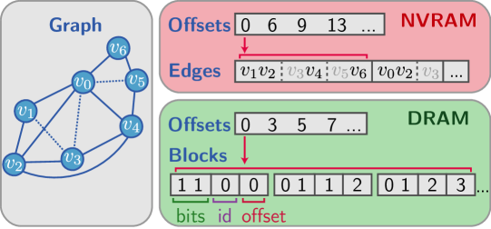
Figure 5: The graph data is stored in the compressed sparse row (CSR) format on NVRAM, and is read-only. Each vertex’s incident edges are logically divided into blocks of size $\mathcal{F}_{B}$ each ($\mathcal{F}_{B}$ = 2 here). The filter is structured similarly to the CSR format and is stored in DRAM. It consists of blocks corresponding to a subset of the logical blocks in the edges array. Each vertex stores a pointer to the start of its blocks, which are stored contiguously. Each filter block stores bits representing the status of the edges in the logical block it corresponds to. In the figure, deleted edges are marked with dotted lines, and correspond to bits set to 0 in the filter. Each block also stores an offset storing the number of active edges (edges with bits set to 1) in all preceding blocks for this vertex, as well as its original block-id, which are both used by our algorithms. When an edge is deleted, its corresponding bit is set to 0, and the offsets of the blocks for the vertex are updated accordingly. The original graph data in stored in the CSR format and is stored on NVRAM and is read-only. On DRAM, we maintain the filter structure that consists of blocks. Each block corresponds to $\mathcal{F}_{B}$ many edges in a consecutive range, and stores $\mathcal{F}_{B}$ many bits for these edges. In addition it stores an offset and the original block-id for each block, which are used by our algorithms. When an edge is deleted, its corresponding bit is set to 0, and the offsets of the blocks for the vertex are updated accordingly. Once a constant fraction of blocks are empty (e.g., the gray block), we physically delete all the empty blocks from the filter structure to guarantee work-efficiency. All writes are on DRAM.

The graph filter’s design mirrors the CSR representation described above. The design of our structure is inspired by similar bit-packed structures, most notably the cuckoo-filter by Eppstein et al. [40]. Figure 5 illustrates the graph filter for the following description.

Definition. The graph data is stored in the compressed sparse row (CSR) format on NVRAM, and is read-only. Each vertex’s incident edges are logically divided into blocks of size $\mathcal{F}_{B}$, the filter block size, which is the provided block size rounded up to the next multiple of the number of bits in a machine word, inclusive (64 bits on modern architectures and $\log n$ bits in theory). In Figure 5, $\mathcal{F}_{B}$ = $2$. For compressed graphs, this block size is always equal to the compression block size (and thus, both must be tuned together).

The filter consists of blocks corresponding to a subset of the logical blocks in the edges array, and is stored in DRAM. Each vertex stores a pointer to the start of its blocks, which are stored contiguously. For each block, the filter stores $\mathcal{F}_{B}{}$ many bits, where the bits correspond one-to-one to the edges in the block. Each block also stores two words of metadata: (i) the original block-ID in the adjacency list that the block corresponds to, and (ii) the offset, which stores the number of active edges before this block. The original block-IDs are necessary because over the course of the algorithm, only a subset of the original blocks used for a vertex may be currently present in the graph filter, and the data structure must remember the original position of each block. The offset is needed for graph primitives which copy all active edges incident to a vertex into an array with size proportional to the degree of the vertex.

The overall graph filter structure thus consists of blocks of bitsets per vertex. It stores the per-vertex blocks contiguously, and stores an offset to the start of each vertex’s blocks. It also stores each vertex’s current degree, as well as the number of blocks in the vertex structure. Finally, the structure stores an additional $n$ bits of memory which are used to mark vertices as dirty.

4.2.2 Algorithms

MakeFilter. To create a graph filter, the algorithm first computes the number of blocks that each vertex requires, based on $\mathcal{F}_{B}$, and writes the space required per vertex into an array. Next, it prefix sums the array, and allocates the required $O(m)$ bits of memory contiguously. It then initializes the per-vertex blocks in parallel, setting all edges as active (their corresponding bit is set to 1). Finally, it allocates an array of $n$ per-vertex structures storing the degree, offset into the bitset structure corresponding to the start of the vertex’s blocks, and the number of blocks for that vertex. Lastly, it initializes per-vertex dirty bits to $\mathsf{false}$ (not dirty) in parallel.

The overall work to create the filter is $O(m)$ and the overall depth is $O(\log n+\mathcal{F}_{B}{})$, because a block is processed sequentially. If the user specifies that the initially supplied predicate returns $\mathsf{false}$ for some edges, the implementation calls filterEdges (described below), which runs within the same work and depth bounds.

PackVertex. Next, we describe an algorithm to pack out the edges incident to a vertex given a predicate $P$. This algorithm is an internal primitive in Sage and is not exposed to the user. The algorithm first maps over all blocks incident to the vertex in parallel.

For each block, it finds all active bits in the block, reads the edge corresponding to the active bit and applies the predicate $P$, unsetting the bit iff the predicate returns $\mathsf{false}$. If the bit for an edge $(u,v)$ is unset, the algorithm marks the dirty bit for $v$ to true if needed. The algorithm maintains a count of how many bits are still active while processing the block, and stores the per-block counts in an array of size equal to the number of blocks. Next, it performs a reduction over this array to compute the number of blocks with at least one active edge. If this value is less than a constant fraction of the current number of blocks incident to the vertex, the algorithm filters out all of these blocks with no active elements, and packs the remaining blocks contiguously in the same memory, using a parallel filter over the blocks. The algorithm then updates the offsets for all blocks using a prefix sum. Finally, the algorithm updates the vertex degree and number of currently active blocks incident to the vertex.

The overall work is $O(A\cdot(\mathcal{F}_{B}{}/\log n)+d_{\emph{active}}(v))$ and the depth is $O(\log n+\mathcal{F}_{B}{})$, where $A$ is the number of non-empty blocks corresponding to $v$ and $d_{\emph{active}}(v)$ is the number of active edges incident to vertex $v$.

edgeMapPack. The edgeMapPack primitive is implemented by applying PackVertex to each vertex in the vertexSubset in parallel. It then updates the number of active edges by performing a reduction over the new vertex degrees in the vertexSubset. The overall work is the sum of the work for packing out each vertex in the vertexSubset, $S$, which is $O(A\cdot(\mathcal{F}_{B}{}/\log n)+\sum_{v\in S}(1+d_{\emph{active}}(v)))$, and the depth is $O(\log n+\mathcal{F}_{B}{})$, where $A$ is the number of non-empty blocks corresponding to all $v\in S$.

filterEdges. The filterEdges primitive uses the edgeMapPack, providing a vertexSubset containing all vertices. The work is $O(n+A\cdot(\mathcal{F}_{B}{}/\log n)+|E_{active}|)$, and the depth is $O(\log n+\mathcal{F}_{B}{})$, where $A$ is the number of non-empty blocks in the graph and $E_{active}$ is the set of active edges represented by the graph filter.

4.2.3 Implementation

Optimizations. We use the widely available tzcnt and blsr x86 intrinsics to accelerate block processing. Each block is logically divided into a number of machine words, so we consider processing a single machine word. If the word is non-zero, we create a temporary copy of the word, and loop while this copy is non-zero. In each iteration, we use tzcnt to find the index of the next lowest bit, and clear the lowest bit using blsr. Doing so allows us to process a block with $q$ words and $k$ non-zero bits in $O(q+k)$ instructions.

We also implemented intersection primitives, which are used in our triangle counting algorithm based on the decoding implementation described above. For compressed graphs, since we may have to decode an entire compressed block to fetch a single active edge, we immediately decompress the entire block and store it locally in the iterator’s memory. We then process the graph filter’s bits word-by-word using the intrinsic-based algorithm described above.

Memory Usage. The overall memory requirement of a graphFilter is $3n$ words to store the degrees, offsets, and number of blocks, plus $O(m)$ bits to store the bitset data and the metadata. The metadata increases the memory usage by a constant factor, since $\mathcal{F}_{B}$ is at least the size of a machine word, and so the metadata stored per block can be amortized against the bits stored in the block. The overall memory usage is therefore $O(n+m/\log n)$ words of memory. For our uncompressed inputs, the size of the graph filter is 4.6–8.1x smaller than the size of the uncompressed graph. For our compressed inputs, the size of the filter is 2.7–2.9x smaller than the size of the compressed graph.

4.3 Semi-Asymmetric Graph Algorithms

We now describe Sage’s efficient parallel graph algorithms in the PSAM model. Our results and theoretical bounds are summarized in Table 1. The bounds are obtained by combining efficient in-memory algorithms in our prior work [37] with the new semi-asymmetric techniques designed in Sections 4.1 and 4.2. We elide some of the details of the theoretical results by describing how the results are obtained based on the proofs from Dhulipala et al. [37]. Specifications of the graph problems and additional algorithm details can be found in Appendix C.

4.3.1 Shortest Path Problems

Algorithms. We consider six shortest-path problems in this paper: breadth-first search (BFS), integral-weight SSSP (wBFS), general-weight SSSP (Bellman-Ford), single-source betweenness centrality, single-source widest path, and $\bm{O(k)}$-spanner. Our BFS, Bellman-Ford, and betweenness centrality implementations are based on those in Ligra [85], and our wBFS implementation is based on the one in Julienne [36]. We provide two implementations of the single-source widest path algorithm, one based on Bellman-Ford, and another based on the wBFS implementation from Julienne [36]. An $O(k)$-spanner is a subgraph that preserves shortest-path distances within a factor of $O(k)$. Our $O(k)$-spanner implementation is based on an algorithm by Miller et al. [69].

Efficiency in the PSAM. Our theoretical bounds for these problems in the PSAM are obtained by using the edgeMapChunked primitive (Section 4.1) for performing sparse graph traversals, because all of these algorithms can be expressed as iteratively performing edgeMapChunked over subsets of vertices. The proofs are similar to the proof we provide for BFS in Section 4.1.3 and rely on Theorem 4.1. Note that the bucketing data structure used in Julienne [36] requires only $O(n)$ words of space to bucket vertices, and thus automatically fits in the PSAM model. The Miller et al. construction builds an $O(k)$-spanner with size $O(n^{1+1/k})$, and runs in $O(m)$ expected work and $O(k\log n)$ depth whp. Our implementation in Sage runs our low-diameter decomposition algorithm, which is efficient in the PSAM as we describe below. We set $k$ to be $\Theta(\log n)$, which results in a spanner with size $O(n)$.

4.3.2 Connectivity Problems

Algorithms. We consider four connectivity problems in this paper: low-diameter decomposition (LDD), connectivity, spanning forest, and biconnectivity. Our implementations are extensions of the implementations provided in GBBS [37].

Efficiency in the PSAM. First, we replace the calls to edgeMapBlocked in each algorithm with calls to edgeMapChunked, which ensures that the graph traversal step uses $O(n)$ words of small-memory using Theorem 4.1. This modification results in PSAM algorithms for LDD. For the other connectivity-like algorithms that use LDD, namely connectivity, spanning forest, biconnectivity, we use the improved analysis of LDD provided in [69] to argue that the number of inter-cluster edges after applying LDD with $\beta=O(1)$ is $O(n)$ in expectation. Thus, the graph on the inter-cluster edges can be built in small-memory. We provide the full details in Appendix C.2. We also obtain the same space bounds in the worst case for our connectivity, spanning forest, biconnectivity, and $O(k)$-spanner algorithms without affecting the work and depth of the algorithms (see Appendix C.2 for details). Lastly, we note that although this results in only $O(n)$ words of small-memory theoretically, in practice our implementation of biconnectivity instead uses the graph filtering structure to optimize a call to connectivity that runs on the input graph, with a large subset of the edges removed.

4.3.3 Covering Problems

Algorithms. We consider four covering problems in this paper: maximal independent set (MIS), maximal matching, graph coloring, and approximate set cover. All of our implementations are extensions of our previous work in GBBS [37].

Efficiency in the PSAM. For MIS and graph coloring, we derive PSAM algorithms by applying our edgeMapChunked optimization because other than graph traversals, both algorithms already use $O(n)$ words of small-memory. Both maximal matching and approximate set cover use our graph filtering technique to achieve immutability and reduced memory usage without affecting the theoretical bounds of the algorithms. We provide more details about our maximal matching algorithm in Appendix C.3. For set cover, our new bounds for filtering match the bounds on filtering used in the GBBS code which mutates the underlying graph, and so our implementation also computes a $(1+\epsilon)$-approximate set cover in $O(m)$ expected work and $O(\log^{3}n)$ depth whp.

4.3.4 Substructure Problems

Algorithms. We consider three substructure-based problems in this paper: $\bm{k}$-core, approximate densest subgraph and triangle counting. Substructure problems are fundamental building blocks for community detection and network analysis (e.g., [24, 49, 58, 79, 80, 100]). Our $k$-core and triangle-counting implementations are based on the implementation from GBBS [37].

Efficiency in the PSAM. For the $k$-core algorithm to use $O(n)$ words of small-memory, it should use the fetch-and-add based implementation of $k$-core, which performs atomic accumulation in an array in order to update the degrees. However, the fetch-and-add based implementation performs poorly in practice, where it incurs high contention to update the degrees of vertices incident to many removed vertices [37]. Therefore, in practice we use a histogram-based implementation, which always runs faster than the fetch-and-add based implementation (the histogram primitive is fully described in [37]). In this paper, we implemented a dense version of the histogram routine, which performs reads for all vertices in the case where the number of neighbors of the current frontier is higher than a threshold $t$. The work of the dense version is $O(m)$. Using $t=m/c$ for some constant $c$ ensures work-efficiency, and results in low memory usage for sparse calls in practice. Our approximate densest subgraph algorithm is similar to our $k$-core algorithm, and uses a histogram to accelerate processing the removal of vertices. The code uses the dense histogram optimization described above. Our triangle counting implementation uses the graph filter structure to orient edges in the graph from lower degree to higher degree.

4.3.5 Eigenvector Problems

Algorithms. We consider the PageRank algorithm, designed to rank the importance of vertices in a graph [25]. Our PageRank implementation is based on the implementation from Ligra.

Efficiency in the PSAM. We optimized the Ligra implementation to improve the depth of the algorithm. The implementation from Ligra runs dense iterations, where the aggregation step for each vertex (reading its neighbor’s PageRank contributions) is done sequentially. In Sage, we implemented a reduction-based method that reduces over these neighbors using a parallel reduce. Therefore, each iteration of our implementation requires $O(m)$ work and $O(\log n)$ depth. The overall work is $O(P_{it}\cdot m)$ and depth is $O(P_{it}\log n)$, where $P_{it}$ is the number of iterations required to run PageRank to convergence with a convergence threshold of $\epsilon=10^{-6}$.

5 Experiments

Overview of Results. After describing the experimental setup (Section 5.1), we show the following main experimental results:

• Section 5.2: Our NUMA-optimized graph storage approach outperforms naive (and natural) approaches by 6.2x.

• Section 5.3: Sage achieves between 31–51x speedup for shortest path problems, 28–53x speedup for connectivity problems, 16–49x speedup for covering problems, 9–63x speedup for substructure problems and 42–56x speedup for eigenvector problems.

• Section 5.4: Compared to existing state-of-the-art DRAM-only graph analytics, Sage run on NVRAM is 1.17x faster on average on our largest graph that fits in DRAM. Sage run on NVRAM is only 5% slower on average than when run entirely in DRAM.

• Section 5.5: We study how Sage compares to other NVRAM approaches for graphs that are larger than DRAM. We find that Sage on NVRAM using App-Direct Mode is 1.94x faster on average than the recent state-of-the-art Galois codes [43] run using Memory Mode. Compared to GBBS codes run using Memory Mode, Sage is 1.87x faster on average across all 18 problems.

• Section 5.6: We compare Sage with existing state-of-the-art semi-external memory graph processing systems, including FlashGraph, Mosaic, and GridGraph and find that our times are 9.3x, 12x, and 8024x faster on average, respectively.

5.1 Experimental Setup

5.1.1 Machine Configuration

We run our experiments on a 48-core, 2-socket machine (with two-way hyper-threading) with $2\times 2.2\mbox{Ghz}$ Intel 24-core Cascade Lake processors (with 33MB L3 cache) and 375GB of DRAM. The machine has 3.024TB of NVRAM spread across 12 252GB DIMMs (6 per socket). All of our speedup numbers report running times on a single thread (T1) divided by running times on 48-cores with hyper-threading (T96). Our programs are compiled with the g++ compiler (version 7.3.0) with the -O3 flag. We use the command numactl -i all for our parallel experiments. Our programs use a work-stealing scheduler that we implemented, implemented similarly to Cilk [21].

Table 2: Graph inputs, number of vertices, edges, and average degree ($d_{\textit{avg}}$).

Graph Dataset	Num. Vertices	Num. Edges	$d_{\textit{avg}}$
LiveJournal [23]	4,847,571	85,702,474	17.6
com-Orkut [104]	3,072,627	234,370,166	76.2
Twitter [54]	41,652,231	2,405,026,092	57.7
ClueWeb [23]	978,408,098	74,744,358,622	76.3
Hyperlink2014 [68]	1,724,573,718	124,141,874,032	72.0
Hyperlink2012 [68]	3,563,602,789	225,840,663,232	63.3

5.1.2 NVRAM Configuration

NVRAM Modes. The NVRAM we use (Optane DC Persistent Memory) can be configured in two distinct modes. In Memory Mode, the DRAM acts like a direct-mapped cache between L3 and the NVRAM for each socket. Memory Mode transparently provides access to higher memory capacity without software modification. In this mode, the read-write asymmetry of NVRAM is obscured by the DRAM cache, and causes the DRAM hit rate to dominate memory performance. In App-Direct Mode, NVRAM acts as byte-addressable storage independent of DRAM, providing developers with direct access to the NVRAM.

Sage Configuration. In Sage, we configure the NVRAM to use App-Direct Mode. The devices are configured using the fsdax mode, which removes the page cache from the I/O path for the device and allows mmap to directly map to the underlying memory.

Graph Storage. The approach we use in Sage is to store two separate copies of the graph, one copy on the local NVRAM of each socket. Threads can determine which socket they are running on by reading a thread-local variable, and access the socket-local copy of the graph. We discuss the approach in detail in Section 5.2

5.1.3 Graph Data

To show how our algorithms perform on graphs at different scales, we selected a representative set of real-world graphs of varying sizes. These graphs are Web graphs and social networks, which are low-diameter graphs that are frequently used in practice. We list the graphs used in our experiments in Table 5.1.1, which we symmetrized to obtain larger graphs and so that all of the algorithms would work on them. Hyperlink 2012 is the largest publicly-available real-world graph. We create weighted graphs for evaluating weighted BFS, Bellman-Ford, and Widest Path by selecting edge weights in the range $[1,\log n)$ uniformly at random. We process the ClueWeb, Hyperlink2014, and Hyperlink2012 graphs in the parallel byte-encoded compression format from Ligra+ [87], and process LiveJournal, com-Orkut, and Twitter in the uncompressed (CSR) format.

5.2 Graph Layout in NVRAM

While building Sage, we observed startingly poor performance of cross-socket reads to graph data stored on NVRAM. We designed a simple micro-benchmark that illustrates this behavior. The benchmark runs over all vertices in parallel. For the $i$-th vertex, it counts the number of neighbors incident to it by reducing over all of its incident edges. It then writes this value to an array location corresponding to the $i$-th vertex. The graph is stored in CSR format, and so the benchmark reads each vertex offset exactly once, and reads the edges incident to each vertex exactly once. Therefore the total number of reads from the NVRAM is proportional to $n+m$, and the number of (in-memory) writes is proportional to $n$.

For the ClueWeb graph, we observed that running the benchmark with the graph on one socket using all 48 hyper-threads on the same socket results in a running time of 7.1 seconds. However, using numactl -i all, and running the benchmark on all threads across both sockets results in a running time of 26.7 seconds, which is 3.7x worse, despite using twice as many hyper-threads. While we are uncertain as to the underlying reason for this slowdown, one possible reason could be the granularity size for the current generation of NVRAM DIMMs, which have a larger effective cache line size of 256 bytes [50], and a relatively small cache within the physical NVM device. Using too many threads could cause thrashing, which is a possible explanation of the slowdowns we observed when scaling up reads to a single NVRAM device by increasing the number of threads. To the best of our knowledge, this significant slowdown has not been observed before, and understanding how to mitigate it is an interesting question for future work.

As described earlier, our approach in Sage is to store two separate copies of the graph, one on the local NVRAM of each socket. Using this configuration, our micro-benchmark runs in 4.3 seconds using all 96 hyper-threads, which is 1.6x faster than the single-socket experiment and 6.2x faster than using threads across both sockets to the graph stored locally within a single socket.

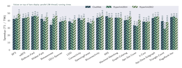
Figure 6: Speedup of Sage algorithms on large graph inputs on a 48-core machine (with 2-way hyper-threading), measured relative to the algorithm’s single-thread time. All algorithms are run using NVRAM in App-Direct Mode. Each bar is annotated with the parallel running time on top of the bar.

5.3 Scalability

Figure 6 shows the speedup obtained on our machine for Sage implementations on our large graphs, annotating each bar with the parallel running time. In all of these experiments, we store all of the graph data in NVRAM and use DRAM for all temporary data.

Shortest Path Problems. Our BFS, weighted BFS, Bellman-Ford, and betweenness centrality implementations achieve between parallel speedups of 31–51x across all inputs. For $O(k)$-Spanner, we achieve 39–51x speedups across all inputs. All Sage codes use the memory-efficient sparse traversal (i.e., edgeMapChunked) designed in this paper. We note that the new weighted-SSSP implementations using edgeMapChunked are up to 2x more memory-efficient than the implementations from [37]. We ran our $O(k)$-Spanner implementation with $k$ set to $\lceil\log_{2}n\rceil$ by default.

Connectivity Problems. Our low-diameter decomposition implementation achieves a speedup of 28–42x across all inputs. Our connectivity and spanning forest implementations, which use the new filtering structure from Section 4.2, achieve speedups of 37–53x across all inputs. Our biconnectivity implementation achieves a speed up of 38–46x across all inputs. We found that setting $\beta=0.2$ in the LDD-based algorithms (connectivity, spanning forest, and biconnectivity) performs best in practice, and creates significantly fewer than $m\beta=m/5$ inter-cluster edges predicted by the theoretical bound [70], due to many duplicate edges that get removed.

Covering Problems. Our MIS, maximal matching, and graph coloring implementations achieve speedups of 43–49x, 33–44x, and 16–39x, respectively. Our MIS implementation is similar to the implementation from GBBS. Our maximal matching implementation implements several new optimizations over the implementation from GBBS, such as using a parallel hash table to aggregate edges that will be processed in a given round. These optimizations result in our code (using the graph filter) running faster than the original code when run in DRAM-only, outperforming the 72-core DRAM-only times reported in [37] for some graphs (we discuss the speedup of Sage over GBBS in Section 5.4).

Substructure Problems. Our $k$-core, approximate densest subgraph, and triangle counting implementations achieve speedups of 9–38x, 43–48x, and 29–63x, respectively. Our code achieves similar speedups and running times on NVRAM compared to the previous times reported in [37]. We ran the approximate densest subgraph implementation with $\epsilon=0.001$, which produces subgraphs of similar density to the $2$-approximation of Charikar [28]. Lastly, the Sage triangle counting algorithm uses the iterator defined over graph filters to perform parallel intersection. The performance of our implementation is affected by the number of edges that must be decoded for compressed graph inputs, and we discuss this in detail in Appendix D.1.

Eigenvector Problems. Our PageRank implementation achieves a parallel speedup of 42–56x. Our implementation is based on the PageRank implementation from Ligra, and improves the parallel scalability of the Ligra-based code by aggregating the neighbor’s contributions for a given vertex in parallel. We ran our PageRank implementation with $\epsilon=10^{-6}$ and a damping factor of $0.85$.

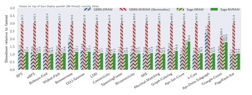
Figure 7: Performance of Sage on the ClueWeb graph compared with existing state-of-the-art in-memory graph processing systems in terms of slowdown relative to the fastest system (smaller is better). GBBS refers to the DRAM-only codes developed in [37], and Sage refers to the codes developed in this paper. Both codes are run in two configurations: DRAM measures the running time when the graph is stored in memory, and NVRAM measures the running time when the graph is stored in non-volatile memory, and accessed either using the techniques developed in this paper (Sage-NVRAM) or using libvmmalloc to automatically convert the DRAM-only codes from GBBS to work using non-volatile memory (GBBS-NVRAM). We truncate relative times slower than 3x and mark the tops of these bars with $*$. All bars are annotated with the parallel running times of the codes on a 48-core system with 2-way hyper-threading. Note that the ClueWeb graph is the largest graph dataset studied in this paper that fits in the main memory of this machine.

5.4 NVRAM vs. DRAM Performance

In this section, we study how fast Sage is compared to state-of-the-art shared-memory graph processing codes, when these codes are run entirely in DRAM. For these experiments, we study the ClueWeb graph since it is the largest graph among our inputs where both the graph and all intermediate algorithm-specific data fully resides in the DRAM of our machine. We consider the following configurations:

1. GBBS codes run entirely in DRAM

2. GBBS codes converted to use NVRAM using libvmmalloc (a robust NVRAM memory allocator)

3. Sage codes run entirely in DRAM

4. Sage codes run using NVRAM in App-Direct Mode

Setting (2) is relevant since it captures the performance of a naive approach to obtaining NVRAM-friendly code, which is to simply run existing shared-memory code using a NVRAM memory allocator.

Figure 7 displays the results of these experiments. Comparing Sage to GBBS when both systems are run in memory shows that our code is faster than the original GBBS implementations by 1.17x on average (between 2.38x faster to 1.73x slower). The notable exception is for triangle counting, where Sage is 1.73x slower than the GBBS code (both run in memory). The reason for this difference is due to the input-ordering the graph is provided in, and is explained in detail in Appendix D.1. A number of Sage implementations, like connectivity and approximate densest subgraph, are faster than the GBBS implementations due to optimizations in our codes that are absent in GBBS, such as a faster implementation of graph contraction. Our read-only codes when run using NVRAM are only about 5% slower on average than when run using DRAM-only. This difference in performance is likely due to the higher cost of NVRAM reads compared to DRAM reads. Finally, Sage is always faster than GBBS when run on NVRAM using libvmmalloc, and is 6.69x faster on average.

These results show that for a wide range of parallel graph algorithms, Sage significantly outperforms a naive approach that converts DRAM codes to NVRAM ones, is often faster than the fastest DRAM-only codes when run in DRAM, and is competitive with the fastest DRAM-only running times when run in NVRAM.

5.5 Alternate NVRAM approaches

We now compare Sage to the fastest available NVRAM approaches when the input graph is larger than the DRAM size of the machine. We focus on the Hyperlink2012 graph, which is our only graph where both the graph and intermediate algorithm data are larger than DRAM. We first compare Sage to the Galois-based implementations by Gill et al. [43], which use NVRAM configured in Memory Mode. We then compare Sage to the unmodified shared-memory codes from GBBS modified to use NVRAM configured in Memory Mode.

Comparison with Galois [43]. Gill et al. [43] study the performance of several state-of-the-art graph processing systems, including Galois [72], GBBS [37], GraphIt [107], and GAP [9] when run on NVRAM configured to use Memory Mode. Their experiments are run on a nearly identical machine to ours, with the same amount of DRAM. However, their machine has 6.144TB of NVRAM (12 NVRAM DIMMs with 512GB of capacity each).

Gill et al. [43] find that their Galois-based codes outperform GAP, GraphIt, and GBBS by between 3.8x, 1.9x, and 1.6x on average, respectively, for three large graphs inputs, including the Hyperlink2012 graph. In our experiments running GBBS on NVRAM using MemoryMode, we find that the GBBS performance using MemoryMode is 1.3x slower on average than Galois. There are several possible reasons for the small difference. First, Gill et al. [43] use the directed version of the Hyperlink2012 graph, which has 1.75x fewer edges than the symmetrized version (225.8B vs. 128.7B edges). The symmetrized graph exhibits a massive connected component containing 94% of the vertices, which a graph search algorithm must process for most source vertices. However, a search from the largest SCC in the directed graph reaches about half the vertices [67]. Second, they do not enable compression in GBBS, which is important for reducing the number of cache-misses and NVRAM reads. Lastly, we found that transparent huge pages (THP) significantly improves performance, while they did not, which may be due to differences regarding THP configuration on the different machines.

Figure 1 shows results for their Galois-based system on the directed Hyperlink2012 graph. Compared with their NVRAM codes, Sage is 1.04–3.08x faster than their fastest reported times, and 1.94x faster on average. Their codes use the maximum degree vertex in the directed graph as the source for BFS, SSSP, and betweenness centrality. We use the maximum degree vertex in the symmetric graph, and note that running on the symmetric graph is more challenging, since our codes must process more edges.

Despite the fact that our algorithm must perform more work, our running times for BFS are 3.08x faster than the time reported for Galois, and our SSSP time is 1.43x faster. For connectivity and PageRank, our times are 2.09x faster and 2.12x faster respectively. For betweenness, our times are 1.04x faster. The authors also report running times for an implementation of $k$-core that computes a single $k$-core, for a given value of $k$. This requires significantly fewer rounds than the $k$-core computation studied in this paper, which computes the coreness number of every vertex, or the largest $k$ such that the vertex participates in the $k$-core. They report that their code requires 49.2 seconds to find the $100$-core of the Hyperlink2012 graph. Our code finds all $k$-cores of this graph in 259 seconds, which requires running 130,728 iterations of the peeling algorithm and also discovers the value of the largest $k$-core supported by the graph ($k_{\max}=10565$).

In summary, we find that using Sage on NVRAM using App-Direct Mode is 1.94x faster on average than the Galois codes run using Memory Mode.

Algorithms using Memory Mode. Next, we compare Sage to the unmodified shared-memory codes from GBBS modified to use NVRAM configured in Memory Mode. We run these Memory Mode experiments on the same machine with 3TB of NVRAM, where 1.5TB is configured to be used in Memory Mode.

Figure 1 reports the parallel running times of both Sage codes using NVRAM, and the GBBS codes using NVRAM configured in Memory Mode for the Hyperlink2012 graph. The results show that in all but one case (triangle counting) our running times are faster (between 1.15–2.92x). For triangle counting, the directed version of the Hyperlink2012 graph fits in about 180GB of memory, which fits within the DRAM of our machine and will therefore reside in memory. We note that we also ran Memory Mode experiments on the ClueWeb graph, which fits in memory. The running times were only 5–10% slower compared to the DRAM-only running times for the same GBBS codes reported in Figure 7, indicating a small overhead due to Memory Mode when the data fits in memory.

In summary, our results for this experiment show that the techniques developed in this paper produce meaningful improvements (1.87x speedup on average, across all 18 problems) over simply running unmodified shared-memory graph algorithms using Memory Mode to handle graph sizes that are larger than DRAM.

5.6 External and Semi-External Systems

In this section we place Sage’s performance in context by comparing it to existing state-of-the-art semi-external memory graph processing systems. Table 5.6 shows the running times and system configurations for state-of-the-art results on semi-external memory graph processing systems. We report the published results presented by the authors of these systems to give a high-level comparison due to the fact that (i) our machine does not have parallel SSD devices that most of these systems require, and (ii) modifying them to use NVRAM would be a serious research undertaking in its own right.

Table 3: System configurations (memory in terabytes and threads (hyper-threads)) and running times (seconds) of existing semi-external memory results on the Hyperlink graphs. The last section shows our running times (note that our system is also equipped with NVRAM DIMMs). *These problems are run on directed versions of the graph.

Paper	Problem	Graph	Mem	Threads	Time
FlashGraph [108]	BFS*	2012	.512	64	208
	BC*	2012	.512	64	595
	Connectivity*	2012	.512	64	461
	PageRank*	2012	.512	64	2041
	TC*	2012	.512	64	7818
Mosaic [62]	BFS*	2014	0.768	1000	6.55
	Connectivity*	2014	0.768	1000	708
	PageRank (1 iter.)*	2014	0.768	1000	21.6
	SSSP*	2014	0.768	1000	8.6
Sage	BFS	2014	0.375	96	5.10
	SSSP	2014	0.375	96	32.8
	Connectivity	2014	0.375	96	15.8
	PageRank (1 iter.)	2014	0.375	96	8.99
	BFS	2012	0.375	96	11.4
	BC	2012	0.375	96	53.9
	Connectivity	2012	0.375	96	36.2
	SSSP	2012	0.375	96	82.3
	PageRank	2012	0.375	96	827
	TC	2012	0.375	96	3529

FlashGraph. FlashGraph [108] is a semi-external memory graph engine that stores vertex data in memory and stores the edge lists in an array of SSDs. Their system is optimized for I/Os at a flash page granularity (4KB), and merges I/O requests to maximize throughput. FlashGraph provides a vertex-centric API, and thus cannot implement some of the work-optimal algorithms designed in Sage, like our connectivity, biconnectivity, or parallel set cover algorithms.

We report running times for FlashGraph for Hyperlink2012 on a 32-core 2-way hyper-threaded machine with 512GB of memory and 15 SSDs in Table 5.6). Compared to FlashGraph, the Sage times are 9.3x faster on average. Our BFS and BC times are 18.2x and 11x faster, and our connectivity, PageRank and triangle counting implementations are 12.7x, 2.4x faster, and 2.2x faster, respectively. We note that our times are on the symmetric version of the Hyperlink2012 graph which has twice the edges, where a BFS from a random seed hits the massive component containing 95% of the vertices (BFSes on the directed graph reach about 30% of the vertices).

Mosaic. Mosaic [62] is a hybrid engine supporting semi-external memory processing based on a Hilbert-ordered data structure. Mosaic uses co-processors (Xeon Phis) to offload edge-centric processing, allowing host processors to perform vertex-centric operations. Giving a full description of their complex execution strategy is not possible in this space, but at a high level, it is based on exploiting the fact that user-programs are written in a vertex-centric model.

We report the running times for Mosaic run using 1000 hyper-threads, 768GB of RAM, and 6 NVMes in Table 5.6. Compared with their times, Sage is 12x faster on average, solving BFS 1.2x faster, connectivity 44.8x faster, SSSP 3.8x slower, and 1-iteration of PageRank 2.4x faster. Given that both SSSP and PageRank are implemented using an SpMV like algorithm in their system, we are not sure why their PageRank times are 2.5x slower than the total time of an SSSP computation. In our experiments, the most costly iteration of Bellman-Ford takes roughly the same amount of time as a single PageRank iteration since both algorithms require similar memory accesses in this step. Sage solves a much broader range of problems compared to Mosaic, and is often faster than it.

GridGraph. GridGraph is an out-of-core graph engine based on a 2-dimensional grid representation of graphs. Their processing scheme ensures that only a subset of the vertex-values accessed and written to are in memory at a given time. GridGraph also offers a mechanism similar to edge filtering which prevents streaming edges from disk if they are inactive. Like FlashGraph, GridGraph is a vertex-centric system and thus cannot implement algorithms that do not fit in this restricted computational model.

The authors consider significantly smaller graphs than those used in our experiments (the largest is a 6.64B edge WebGraph). However, they do solve the LiveJournal and Twitter graphs that we use. For the Twitter graph, our BFS and Connectivity times are 15690x and 359x faster respectively than theirs (our speedups for LiveJournal are similar). GridGraph does not use direction optimization, which is likely why their BFS times are much slower.

6 Related Work

A significant amount of research has focused on reducing expensive writes to NVRAMs. Early work has designed algorithms for database operators [30, 97, 98]. Blelloch et al. [10, 15, 16] define computational models to capture the asymmetric read-write cost on NVRAMs, and many algorithms and lower bounds have been obtained based on the models [11, 19, 20, 46, 51]. Other models and systems to reduce writes or memory footprint on NVRAMs have also been described [5, 6, 26, 27, 29, 55, 61, 73, 74, 81, 95].

Persistence is a key property of NVRAMs due to their non-volatility. Many new persistent data structures have been designed for NVRAMs [7, 12, 31, 32, 75, 84]. There has also been research on automatic recovery schemes and transactional memory for NVRAMs [3, 34, 56, 60, 99, 106, 110]. There are several recent papers benchmarking performance on NVRAMs [50, 59, 96].

Parallel graph processing frameworks have received significant attention due to the need to quickly analyze large graphs [78]. The only previous graph processing work targeting NVRAMs is the concurrent work by Gill et al. [43], which we discuss in Section 5.5. Dhulipala et al. [36, 37] design the Graph Based Benchmark Suite, and show that the largest publicly-available graph, the Hyperlink2012 graph, can be efficiently processed on a single multicore machine. We compare with these algorithms in Section 5. Other multicore frameworks include Galois [72], Ligra [85, 87], Polymer [105], Gemini [111], GraphGrind [90], Green-Marl [48], Grazelle [44], and GraphIt [107]. We refer the reader to [4, 63, 83, 103] for excellent surveys of this growing literature.

7 Conclusion

We have introduced Sage, which takes a semi-asymmetric approach to designing parallel graph algorithms that avoid writing to the NVRAM and uses DRAM proportional to the number of vertices. We have designed a new model, the Parallel Semi-Asymmetric Model, and have shown that all of our algorithms in Sage are provably efficient, and often work-optimal in the model. Our empirical study shows that Sage graph algorithms can bridge the performance gap between NVRAM and DRAM. This enables NVRAMs, which are more cost-efficient and support larger capacities than traditional DRAM, to be used for large-scale graph processing. Interesting directions for future work include studying which filtering algorithms can be made to use only $O(n)$ words of DRAM, and to study how Sage performs relative to existing NVRAM graph-processing approaches on synthetic graphs with trillions of edges.

Appendix A Memory-Efficient Parallel Graph Traversal

In this section, we provide additional details on Sage’s memory-efficient parallel graph traversal algorithm. The algorithm description uses the parallel primitives defined in Section 2.

Chunked Parallel Traversal. In Sage, we use a chunk-based method to optimize the memory-efficiency of the sparse (push-based) edgeMap. Our approach, which we refer to as edgeMapChunked, shares some similarities, and achieves the same cache performance as the edgeMapBlocked implementation used in GBBS [37], but crucially it improves the intermediate memory usage.

We provide pseudocode for our algorithm in Algorithm 1. The algorithm is based on three types of chunking. First, the algorithm breaks up the edges incident to each vertex into blocks based on the underlying graph’s block size. Second, the algorithm chunks the outgoing edges to traverse, which it breaks up into groups. Each group consists of some number of blocks. The blocks within a group will be processed sequentially, but different groups can be processed in parallel. Third, the algorithm performs chunking of the output that is generated, writing out the neighbors that must be emitted in the output vertexSubset into fixed-size chunks.

The algorithm first breaks each vertex up into units of work called blocks based on a block size parameter, $G_{\mathit{b\_size}}$ (Line 11). This block size can be tuned arbitrarily for uncompressed graphs, but must be set equal to the compression block size for compressed graphs. Different settings of the block size result in a tradeoff between the depth of the algorithm and the amount of small-memory used in the PSAM model. We discuss this tradeoff, and how to set this block size below. Next, the algorithm decides the number of groups to create (Lines 13–18), where each group consists of a set of blocks. It then processes the groups in parallel. For each group, it processes the blocks within the group one at a time. When starting the next block, it calls the FetchChunk procedure (Lines 4–9), which returns an output chunk for the current group, allocating a fresh chunk if the current chunk is too full (Line 22). Each group stores the chunks allocated for it in a per-group vector of output chunks ($\mathit{V}$ from Line 19), which can be accessed safely without any atomics, since each group is processed by a single thread. The chunk allocations are done in our implementation using a pool-based thread-local allocator (Line 3). Next, the algorithm processes the block and writes all neighbors that should be emitted in the next vertexSubset into the chunk, and updates the block size (Line 23). Note that the FetchChunk procedure ensures that the returned chunk has sufficient space to store all neighbors in the block being processed (Line 6). The remaining steps aggregate the chunks from the per-group vectors (Line 24), perform prefix sum on the chunk sizes (Line 26), and copy the data within the chunks into an array with size proportional to the number of returned neighbors (Lines 28–30). After copying the data within a chunk, the algorithm frees the chunk (Line 30). Finally, the algorithm returns the output vertexSubset (Line 31).

Memory Usage, Work, and Depth. First note that in the degenerate case where all edges are processed using our implementation, the code can create up to $m/G_{\mathit{b\_size}}$ many blocks, which can be $\Omega(n)$. Instead, we ensure that $G_{\mathit{b\_size}}=d_{\emph{avg}}=\lceil m/n\rceil$, or the average degree. In this case, the maximum number of blocks used is $m/G_{\mathit{b\_size}}=m/d_{\emph{avg}}=O(n)$. It is simple to check the remainder of the code and observe that the amount of intermediate memory and the output size are bounded by $O(n)$ words. The overall small-memory usage of the procedure is therefore $O(n)$ words. Note that for compressed graphs, the block size is equal to the compression block size, and thus the compression block size must be set to $d_{\emph{avg}}$ to ensure theoretical efficiency in the PSAM. For uncompressed graphs the block size can be set arbitrarily.

To ensure that we do not create an unnecessarily large number of groups, we set the number of groups to $O(\min(8p,\allowbreak\sum_{u\in U}\emph{deg}(u)/\mathit{min\_group\_size}))$ on $p$ processors (Lines 14–16 and Line 2). These parameters balance between providing enough parallel slackness for work-stealing when there is a large amount of work to be done (the $8p$ term in the $\min$) while also ensuring that we do not over-provision parallelism in the case when the number of edges incident to the frontier is small (the second term in the $\min$).

The overall work of the procedure is $O(\sum_{u\in U}\emph{deg}(u))$, and the overall depth is $O(\log n+\mathit{group\_size})$, since each group is processed sequentially by a single thread, and each call to the procedure requires aggregating the per-group chunks, which can be done in parallel. Note that theoretically, $\mathit{group\_size}=O(d_{\emph{avg}})$ since the $\max$ on Line 15 includes the $\lceil d_{U}/8p\rceil$ only to avoid creating excess groups when parallelism is abundant, and $\mathit{min\_group\_size}=O(d_{\emph{avg}})$ (Line 2). The work done for the chunk-aggregation is proportional to the number of groups (and number of output chunks), both of which are upper-bounded by $O(\sum_{u\in U}\emph{deg}(u))$. $d_{\emph{avg}}$ is usually a small constant in real-world graphs (see Table 5.1.1).

Algorithm 1 edgeMapChunked

1:$\mathit{chunk\_size}=\max(4096,d_{\emph{avg}})$

2:$\mathit{min\_group\_size}=\max(4096,d_{\emph{avg}})$

3:$\mathit{chunk\_alloc}\coloneqq$ Initialize thread-local allocator with $\mathit{chunk\_size}$

4:procedure FetchChunk($\mathit{b\_size}$, $V$)

5:   $\mathit{chunk}\coloneqq$ Last chunk from $V$ $\triangleright$ $V:$ vector of output chunks for this group

6:   if $\mathit{chunk}=\mathsf{null}$ or $\mathit{chunk}.\textsc{size}+b\_size>\mathit{chunk\_size}$ then

7:      $\mathit{chunk}\coloneqq\mathit{chunk\_alloc}.\textsc{allocate}()$

8:      Insert $\mathit{chunk}$ into $V$    

9:   return $\mathit{chunk}$

10:procedure edgeMapChunked($G,U,F$)

11:   $G_{\mathit{b\_size}}\coloneqq d_{\emph{avg}}$ $\triangleright$ underlying block size used in $G$

12:   $\mathit{B}\coloneqq$ Output blocks corresponding to $u\in U$

13:   $\mathit{O}\coloneqq$ Prefix sums of block-degrees for blocks in $B$

14:   $d_{U}\coloneqq\sum_{u\in U}\emph{deg}(u)$

15:   $\mathit{group\_size}\coloneqq\max(\lceil d_{U}/8p\rceil,\mathit{min\_group\_size})$

16:   $\mathit{num\_groups}\coloneqq\lceil d_{U}/\mathit{group\_size}\rceil$

17:   $\mathit{idxs}\coloneqq\{i\cdot\mathit{group\_size}\ |\ i\in[\mathit{num\_groups}]\}$

18:   $\mathit{Offs}\coloneqq$ Offsets into $O$ resulting from a parallel merge of $idxs$ and $O$

19:   $\mathit{V}\coloneqq$ Array of vectors storing chunks of size $\mathit{num\_groups}$

20:   parfor $i$ in $[0,|\mathit{Offs}|)$ do $\triangleright$ In parallel over the groups

21:      for $j$ in $[\mathit{Offs}[i],\mathit{Offs}[i+1])$ do $\triangleright$ $\leq G_{\mathit{b\_size}}$ edges in block $j$

22:         $\mathit{chunk}\coloneqq\textsc{FetchChunk}(G_{\mathit{b\_size}},V_{i})$

23:         Process vertices in block $j$ by applying $F$, and write vertices where $F$ returns $\mathsf{true}$ into $\mathit{chunk}$          

24:   $\mathit{C}\coloneqq$ All chunks extracted from $\mathit{V}$

25:   $\mathit{output\_offsets}\coloneqq$ Array of length $|C|$ where the $i$’th entry contains the size of the $i$’th chunk, $C[i]$

26:   $\mathit{output\_size}\coloneqq$ $\mathit{Scan}(\mathit{output\_offsets},+)$

27:   $\mathit{output}\coloneqq$ Array of size $\mathit{output\_size}$

28:   parfor $c\in\mathit{C}$ do

29:      Copy elements in $c$ to $\mathit{output}$ starting at offset in $\mathit{output\_offsets}$ corresponding to $c$

30:      $\mathit{chunk\_alloc}.\textsc{release}(c)$    

31:   return $\mathit{output}$

Appendix B Semi-Asymmetric Bucketing

We now briefly describe how to adapt the work-efficient bucketing structure from Julienne [36] to the PSAM. A bucketing structure maintains a dynamic mapping between a set of elements and buckets, and is used in several important graph algorithms for work-efficiency: weighted breadth-first search, $k$-core, approximate densest subgraph, and approximate set cover. The bucketing strategy in Julienne is based on lazy bucketing, which avoids deleting the bucketed elements from buckets that they are moved out of. If the elements that are bucketed are the vertices, and the total number of bucket updates is $O(m)$, then the use of lazy bucketing will require the bucket structure to use $O(m)$ words of small-memory, violating the PSAM requirements.

We can address this issue by using semi-eager bucketing. In the semi-eager version, each bucket maintains two counters, storing the number of live (not logically deleted) elements currently in the bucket, and the number of dead (logically deleted) elements. When moving a vertex out of a bucket, we increment the dead element count in that bucket. When a bucket contains more than a constant factor of dead elements, we physically pack them out. Since each vertex is contained in a single bucket, this approach only uses $O(n)$ words of small-memory for bucketing vertices.

In practice, we use the practical variant of the bucketing structure proposed in Julienne [36], which is based on maintaining a constant number of active buckets with the highest priority, and an overflow bucket for all remaining vertices. This approach also uses only $O(n)$ words of small-memory for bucketing vertices.

Appendix C Algorithm Specification and Analysis

This section supplements Section 4.3 with specifications of the problems that we study, and additional algorithm details.

C.1 Shortest Path Problems

We consider six shortest-path problems in this paper: breadth-first search (BFS), integral-weight SSSP (wBFS), general-weight SSSP (Bellman-Ford), single-source betweenness centrality, integral-weight single-source widest path (widest-path), and $O(k)$-spanner. Our implementations of BFS, Bellman-Ford, and betweenness centrality are based on the implementations in Ligra [85], and our wBFS implementation is based on our earlier work on Julienne [36]. We provide two implementations of the widest-path algorithm, one based on Bellman-Ford, and another based on the wBFS implementation from Julienne [36]. As mentioned in Section 4.3.1, we obtain semi-asymmetric algorithms for the first five these problems by using edgeMapChunked (Section 4.1) for performing sparse graph traversals.

Our $O(k)$-spanner implementation is based on a recently described spanner algorithm due to Miller et al. [69]. A $O(k)$-spanner is a subgraph that preserves shortest path distances within a multiplicative factor of $O(k)$. Their construction computes an $O(k)$-spanner with size $O(n^{1+1/k})$, and runs in $O(m)$ expected work and $O(k\log n)$ depth whp. The implementation uses a low-diameter decomposition algorithm, which we describe below. In our experiments, we set $k$ to be $\lceil\log n\rceil$, which gives a spanner that has $O(n)$ size.

C.2 Connectivity Problems

We consider four connectivity problems in this paper: low-diameter decomposition (LDD), connectivity, spanning forest, and biconnectivity. Our implementations in this paper are extensions of the implementations provided in GBBS [37]. We note that connectivity, spanning forest, biconnectivity, and $O(k)$-spanner all use LDD as a subroutine. Our results for connectivity, spanning forest, and biconnectivity work by observing that the low-diameter decomposition primitive used in the work-efficient connectivity algorithm of Shun et al. [86] produces a much larger drop in the number of inter-cluster edges than the original analysis of this algorithm. In particular, the number of inter-cluster edges becomes $O(n)$ in expectation after a single application of LDD. Therefore, we can simply run a single round of LDD, and build the inter-cluster graph in the fast memory after a single round. The specific result we use is Corollary 3.1 of  [69], which we reproduce here for completeness:

Lemma C.1 (Corollary 3.1 of [69])

In an exponential start time decomposition with parameter $\beta=\frac{\log n}{2k}$, for any vertex $v\in V$ the ball $B(v,1)=\{u\in V\ |\ d(u,v)\leq 1\}$ intersects $O(n^{1/k})$ clusters in expectation.

The number of clusters the radius-1 ball around a vertex intersects is exactly the number of inter-cluster edges incident to the vertex. Applying Lemma C.1 with $k=c\log n$, we have that $\beta=\frac{1}{2c}$, for a suitable constant $c$, and that the number of inter-cluster edges incident to $v$ is $O(n^{1/c\log n})=O(1)$ in expectation.

Thus, applying this lemma across all vertices, by linearity the number of inter-cluster edges in $G$ drops to $O(n)$ in expectation after applying the LDD once, when $\beta=\frac{1}{2c}$ for some constant $c$. At this point, the entire graph on $n$ vertices, and all inter-cluster edges can be built in the fast memory, and the previous algorithm of Shun et al. [86] can be run in the fast memory on this new graph. By the analysis above, and the fact that the Shun et al. [86] algorithm runs in $O(m)$ expected work and $O(\log^{3}n)$ depth whp, we have the following result for connectivity in the PSAM.

Theorem C.2

There is a parallel connectivity algorithm that performs $O(m)$ expected work and $O(\log^{3}n)$ depth whp in the PSAM model with $O(n)$ words of memory.

An identical argument holds for spanning forest, and biconnectivity (which uses the connectivity algorithm as a subroutine).

Corollary C.3

There are algorithms for computing spanning forest and biconnectivity that perform $O(m)$ expected work each, and $O(\log^{3}n)$ depth and $O(d_{G}\log n+\log^{3}n)$ depth whp in the PSAM model with $O(n)$ words of memory.

We note that our biconnectivity implementation utilizes the filtering structure (Section 4.2) to accelerate a call to connectivity that operates on a graph with most of the edges removed, and thus our implementation runs in the relaxed PSAM model for practical efficiency.

Handling Restarts in Low-Diameter Decomposition-Based Algorithms. One issue that arises when running in the PSAM is that algorithms which use $O(n)$ words of small-memory in expectation may need to be restarted if the space bound is violated. This situation can occur for several of our algorithms which are based on running a low-diameter decomposition, and contracting, or selecting inter-cluster edges based on the decomposition. In what follows, we focus on the connectivity algorithm, since our spanning forest, biconnectivity, and $O(k)$-spanner algorithm are also handled identically.

In our connectivity algorithm, we can ensure that the algorithm runs in $O(n)$ words of space by re-running the LDD algorithm until it succeeds. Checking whether an LDD succeeds can be done in $O(n)$ space and $O(n+m)$ work by simply counting the number of inter-cluster edges formed by the partition of vertices. Once the LDD succeeds, the rest of the algorithm does not require restarts, since the recursive calls in the connectivity algorithm always fit within $O(n)$ words of space [86]. We note that since the LDD succeeds with constant probability, an expected constant number of iterations are needed for the connectivity algorithm to succeed. Therefore, the work bounds obtained using restarting are still $O(m)$ in expectation. Furthermore, the depth bound is not affected by the restarts since we only need to perform restarts at the first level of recursion in the algorithm. Since we must perform at most $O(\log n)$ restarts at this level to guarantee success whp, the overall contribution to the depth of re-running an LDD at this step is $O(\log^{2}n)$ whp, which is subsumed by the algorithm’s overall depth.

C.3 Covering Problems

We consider four covering problems in this paper: maximal independent set (MIS), maximal matching, graph coloring, and approximate set cover. Our implementations are extensions of the implementations described in [37]. First, for MIS and graph coloring, we derive PSAM algorithms by applying our edgeMapChunked optimization since other than graph traversals, both algorithms already use $O(n)$ words of small-memory. Both maximal matching and approximate set cover require using our graph filtering technique to achieve immutability and reduced memory usage without affecting the theoretical bounds of the algorithms.

Our maximal matching algorithm runs phases of the filtering-based maximal matching algorithm described in [37] on subsets of the edges such that they fit in small-memory. The algorithm has access to $O(n+m/\log n)$ words of memory, so we can solve the problem by extracting the next $O(m/\log n)$ unprocessed edges on each phase, and running the random-priority based maximal matching algorithm on the subset of edges. The algorithm will finish after performing $O(\log n)$ phases. This does not affect the overall work and increases the depth by an $O(\log n)$ factor. The depth of applying maximal matching within a phase is $O(\log^{2}n)$ whp using the analysis of Fischer and Noever [42], combined with the implementation from Blelloch et al. [17]. Thus, the overall depth of the algorithm is $O(\log^{3}n)$ whp. In practice, we use a similar approach that is theoretically motivated and makes use of our graph-filtering structure. In each phase, we extract $O(n)$ unmatched edges, and process them using the random-priority based algorithm [17]. All unmatched edges from this set are discarded, and the graph is filtered using filterEdges to pack out edges incident to matched vertices. Theoretically, we can switch to the previously described version after a constant number of such phases. However, we observed that in practice, a constant number of iterations of the filtering procedure suffices for all graphs that we tested on.

Our approximate set cover implementation is similar to the implementation from [37], with the exception that the underlying filtering is done using a graph filter, instead of mutating the original graph. The bounds obtained for the graph filter structure match the bounds on filtering used in the GBBS code, which mutates the underlying graph, and so our implementation also computes a $(1+\epsilon)$-approximate set cover in $O(m)$ expected work and $O(\log^{3}n)$ depth whp.

C.4 Substructure Problems

We consider three substructure problems in this paper: $k$-core, approximate densest subgraph and triangle counting. Our $k$-core implementation is similar to the implementation from GBBS [37]. We refer to Section 4.3.4 for descriptions of our $k$-core and approximate densest subgraph algorithms.

Our triangle counting code is based on the GBBS implementation, which is an implementation of the parallel triangle counting algorithm from Shun and Tangwongsan [88]. Our implementation uses the graph filter structure to orient edges in the graph from lower degree to higher degree. Since we only require outgoing edges, we supply a flag to the framework which permits it to only represent the outgoing edges of the directed graph, halving the amount of internal memory required. Our implementation uses the new iterator implemented over the graph filter structure to perform intersections between the outgoing edges of two vertices. We note that in our implementation, we perform intersection sequentially, which theoretically guarantees a depth of $O(\sqrt{m})$. However, the parallelism of this algorithm is $O(m^{3/2}/m^{1/2})=O(m)$ which in practice is sufficiently high that reducing the depth using a parallel intersection routine is unnecessary, and can hurt performance due to using a more complicated intersection algorithm.

Theoretically, the bounds for Triangle Counting in Table 1 can be obtained by using a parallel intersection method on the filter structure. The implementation of this idea for the blocked adjacency lists in the filter structure is identical to the $O(\log n)$ depth intersection method defined on compressed graphs in [37]. The idea is similar to the classic parallel intersection, or merge algorithms on two sorted arrays [52, 13].

C.5 PageRank

We consider the PageRank algorithm, designed to rank the importance of vertices in a graph [25]. Our PageRank implementation is described in Section 4.3.5.

Appendix D Experiments

D.1 Graph Filtering and Triangle Counting

We consider the effect that the underlying block size used in the graph filter has on the performance of our triangle counting implementation. Recall that for our compressed inputs, extracting a given edge from a block requires possibly (sequentially) decompressing the full block to retrieve the desired edge. We refer to the work done to decompress edges within the decoded blocks as the total work done by our triangle counting implementation. We note that this measure is a function of both the block size used in the graph filter, as well as the underlying graph ordering. We refer to the work that has to be done to perform all directed intersections as the intersection work done by the triangle counting implementation, not including decoding blocks. Note that the intersection work for a graph is a fixed quantity for a given total ordering of the vertices. The intersection work is a lower bound on the total amount of work that has to be done, but the total amount of work can be much larger if the blocks containing active edges (edges in the directed graph) are spares blocks (e.g., if each block only contains a single active edge).

Graph	Block Size	Intersection Work	Total Work	Time (s)
ClueWeb	64	2.24$\cdot 10^{10}$	7.16$\cdot 10^{10}$	489
ClueWeb	128	2.24$\cdot 10^{10}$	9.54$\cdot 10^{10}$	567
ClueWeb	256	2.24$\cdot 10^{10}$	12.8$\cdot 10^{10}$	683
Hyperlink2014	64	4.8$\cdot 10^{12}$	101$\cdot 10^{12}$	5722
Hyperlink2012	64	10.4$\cdot 10^{12}$	67.2$\cdot 10^{12}$	3529

Table 4: Tradeoff between $\mathcal{F}_{B}$, the graph filter block size, the number of directed wedges that must be checked for this graph (Intersection Work), the total amount of work performed decoding edges within blocks in triangle counting (Total Work), and the running time of triangle counting for the ClueWeb graph. The second half of the table reports the same statistics for the Hyperlink2014 and Hyperlink2012 graphs for the configurations in which our reported running times in Figure 6 were run.

Table 4 reports numbers displaying this tradeoff between the $\mathcal{F}_{B}$, the graph filter block size, total amount of work required to decode all edges within blocks, and the running time of the implementation. We observe that using a smaller $\mathcal{F}_{B}$ results in a more work-efficient implementation, which directly translates to a faster running time. We chose to use a block size of 64 since it provided the best tradeoff between running time on other problems considered in this paper, the size of the compressed graph, and running time for triangle counting.

Finally, Table 4 also reports the block sizes, intersection work and total work required to run triangle counting on the Hyperlink2014 and Hyperlink2012 graph with $\mathcal{F}_{B}{}=64$. Recall that the intersection work is a lower bound on the total amount of work that is done, and that the total work is the amount of decoding operations actually performed by our implementation. We note that triangle counting on the Hyperlink2014 graph incurs a much larger penalty in terms of total work than Hyperlink2012 (1.5x larger). The running time of the code on the Hyperlink2014 graph is also 1.6x larger than the time for the code on Hyperlink2012, which supports the hypothesis that the total work is largely responsible for the running time of the triangle counting intersection.

D.2 Memory Usage of edgeMapChunked

Next, we study the memory improvements in terms of total memory used by the program due to the edgeMapChunked optimization. We report both the total memory used, and the running times for running BFS from a given source vertex within the massive connected component for the ClueWeb and Hyperlink2012 graphs. We compare our implementation to the BFS implementation from GBBS, which uses the edgeMapBlocked algorithm that allocates an intermediate array with size proportional to the number of out-neighbors of a frontier. Both implementations use the same source vertex.

Table 5 shows the results of the experiments. We observe that our new chunk-based implementation requires roughly the same order of magnitude of memory as the previous edgeMapBlocked implementation, and also results in similar running times. Both edgeMapBlocked and edgeMapChunked use significantly less memory than using edgeMapSparse. Specifically, edgeMapChunked uses 1.24x less memory than edgeMapSparse on ClueWeb, 1.27x less memory on Hyperlink2014, and 1.31x less memory on Hyperlink2012. The memory usage between edgeMapChunked and edgeMapBlocked is likely similar since edgeMapBlocked only performs DRAM writes proportional to the output size of edgeMap, which is the same number of writes (and therefore physical pages) as performed by edgeMapChunked.

In addition, using our edgeMapChunked implementation we can run a “sparse-only” edgeMap with limited memory. Although running only the sparse version of a breadth-first search is not particularly practical, it is useful for understanding the performance improvement gained by using Beamer’s direction-optimization on very large real-world graphs. Running a similar sparse-only breadth-first search using either edgeMapSparse or edgeMapBlocked causes a segmentation fault on the Hyperlink2012 graph. The fault occurs because the algorithm tries to allocate an 492GB array from DRAM, which is larger than the DRAM size of our machine. In contrast, our edgeMapChunked-based implementation successfully runs in 38.8s and has a peak-memory usage of 120GB of memory, which is less than $1/3$ of our machine’s memory DRAM capacity. Our implementation lets us see that using direction-optimization results in a 3.1x speedup over running the sparse-only code for this graph.

Graph	Algorithm	DRAM Usage	Time (s)
ClueWeb	edgeMapSparse	33.0GB	2.52
ClueWeb	edgeMapBlocked	28.2GB	2.43
ClueWeb	edgeMapChunked	26.6GB	2.35
Hyperlink2014	edgeMapSparse	54.0GB	5.61
Hyperlink2014	edgeMapBlocked	42.7GB	5.20
Hyperlink2014	edgeMapChunked	42.3GB	5.10
Hyperlink2012	edgeMapSparse	115GB	12.5
Hyperlink2012	edgeMapBlocked	90.3GB	12.3
Hyperlink2012	edgeMapChunked	87.5GB	12.2

Table 5: Effect of the sparse traversal algorithm (edgeMapSparse, edgeMapBlocked, and edgeMapChunked) on the total DRAM usage and the running time of our BFS implementation.

References

- [1] J. Abello, A. L. Buchsbaum, and J. R. Westbrook. A functional approach to external graph algorithms. Algorithmica, 32(3):437–458, Mar 2002.
- [2] A. Aggarwal and J. S. Vitter. The Input/Output complexity of sorting and related problems. Commun. ACM, 31(9), 1988.
- [3] M. Alshboul, H. Elnawawy, R. Elkhouly, K. Kimura, J. Tuck, and Y. Solihin. Efficient checkpointing with recompute scheme for non-volatile main memory. ACM Transactions on Architecture and Code Optimization (TACO), 16(2):18, 2019.
- [4] K. Ammar and M. T. Özsu. Experimental analysis of distributed graph systems. PVLDB, 11(10):1151–1164, 2018.
- [5] J. Arulraj, J. Levandoski, U. F. Minhas, and P.-A. Larson. BzTree: A high-performance latch-free range index for non-volatile memory. 2018.
- [6] J. Arulraj and A. Pavlo. How to build a non-volatile memory database management system. In ACM International Conference on Management of Data (SIGMOD), pages 1753–1758, 2017.
- [7] H. Attiya, O. Ben-Baruch, P. Fatourou, D. Hendler, and E. Kosmas. Tracking in order to recover: Recoverable lock-free data structures. CoRR, abs/1905.13600, 2019.
- [8] S. Beamer, K. Asanović, and D. Patterson. Direction-optimizing breadth-first search. In SC, 2012.
- [9] S. Beamer, K. Asanovic, and D. A. Patterson. The GAP benchmark suite. CoRR, abs/1508.03619, 2015.
- [10] N. Ben-David, G. E. Blelloch, J. T. Fineman, P. B. Gibbons, Y. Gu, C. McGuffey, and J. Shun. Parallel algorithms for asymmetric read-write costs. In ACM Symposium on Parallelism in Algorithms and Architectures (SPAA), 2016.
- [11] N. Ben-David, G. E. Blelloch, J. T. Fineman, P. B. Gibbons, Y. Gu, C. McGuffey, and J. Shun. Implicit decomposition for write-efficient connectivity algorithms. In IEEE International Parallel and Distributed Processing Symposium (IPDPS), 2018.
- [12] N. Ben-David, G. E. Blelloch, M. Friedman, and Y. Wei. Delay-free concurrency on faulty persistent memory. In ACM Symposium on Parallelism in Algorithms and Architectures (SPAA), pages 253–264, 2019.
- [13] G. E. Blelloch and L. Dhulipala. Introduction to parallel algorithms 15-853: Algorithms in the real world. 2018.
- [14] G. E. Blelloch, D. Ferizovic, and Y. Sun. Just join for parallel ordered sets. In ACM Symposium on Parallelism in Algorithms and Architectures (SPAA), 2016.
- [15] G. E. Blelloch, J. T. Fineman, P. B. Gibbons, Y. Gu, and J. Shun. Sorting with asymmetric read and write costs. In ACM Symposium on Parallelism in Algorithms and Architectures (SPAA), 2015.
- [16] G. E. Blelloch, J. T. Fineman, P. B. Gibbons, Y. Gu, and J. Shun. Efficient algorithms with asymmetric read and write costs. In European Symposium on Algorithms (ESA), 2016.
- [17] G. E. Blelloch, J. T. Fineman, and J. Shun. Greedy sequential maximal independent set and matching are parallel on average. In ACM Symposium on Parallelism in Algorithms and Architectures (SPAA), 2012.
- [18] G. E. Blelloch, J. T. Fineman, Y. Gu, and Y. Sun. Optimal parallel algorithms in the binary-forking model. In ACM Symposium on Parallelism in Algorithms and Architectures (SPAA), 2020.
- [19] G. E. Blelloch and Y. Gu. Improved parallel cache-oblivious algorithms for dynamic programming. In SIAM/ACM Symposium on Algorithmic Principles of Computer Systems (APOCS), pages 105–119, 2020.
- [20] G. E. Blelloch, Y. Gu, J. Shun, and Y. Sun. Parallel write-efficient algorithms and data structures for computational geometry. In ACM Symposium on Parallelism in Algorithms and Architectures (SPAA), 2018.
- [21] R. D. Blumofe, C. F. Joerg, B. C. Kuszmaul, C. E. Leiserson, K. H. Randall, and Y. Zhou. Cilk: An efficient multithreaded runtime system. In ACM Symposium on Principles and Practice of Parallel Programming (PPOPP), 1995.
- [22] R. D. Blumofe and C. E. Leiserson. Scheduling multithreaded computations by work stealing. J. ACM, 46(5):720–748, 1999.
- [23] P. Boldi and S. Vigna. The WebGraph framework I: Compression techniques. In Proc. of the Thirteenth International World Wide Web Conference (WWW 2004), pages 595–601, 2004.
- [24] F. Bonchi, A. Khan, and L. Severini. Distance-generalized core decomposition. In ACM International Conference on Management of Data (SIGMOD), 2019.
- [25] S. Brin and L. Page. The anatomy of a large-scale hypertextual web search engine. In International World Wide Web Conference (WWW), pages 107–117, 1998.
- [26] T. Cai, F. Chen, Q. He, D. Niu, and J. Wang. The matrix KV storage system based on NVM devices. Micromachines, 10(5):346, 2019.
- [27] E. Carson, J. Demmel, L. Grigori, N. Knight, P. Koanantakool, O. Schwartz, and H. V. Simhadri. Write-avoiding algorithms. In IEEE International Parallel and Distributed Processing Symposium (IPDPS), 2016.
- [28] M. Charikar. Greedy approximation algorithms for finding dense components in a graph. In International Workshop on Approximation Algorithms for Combinatorial Optimization, pages 84–95, 2000.
- [29] Q. Chen, H. Lee, Y. Kim, H. Y. Yeom, and Y. Son. Design and implementation of skiplist-based key-value store on non-volatile memory. Cluster Computing, 22(2):361–371, 2019.
- [30] S. Chen, P. B. Gibbons, and S. Nath. Rethinking database algorithms for phase change memory. In Conference on Innovative Data Systems Research (CIDR), 2011.
- [31] S. Chen and Q. Jin. Persistent B+-trees in non-volatile main memory. PVLDB, 8(7):786–797, 2015.
- [32] N. Cohen, R. Guerraoui, and M. I. Zablotchi. The inherent cost of remembering consistently. In ACM Symposium on Parallelism in Algorithms and Architectures (SPAA), 2018.
- [33] T. H. Cormen, C. E. Leiserson, R. L. Rivest, and C. Stein. Introduction to Algorithms (3. ed.). MIT Press, 2009.
- [34] A. Correia, P. Felber, and P. Ramalhete. Romulus: Efficient algorithms for persistent transactional memory. In ACM Symposium on Parallelism in Algorithms and Architectures (SPAA), pages 271–282, 2018.
- [35] T. A. Davis and Y. Hu. The University of Florida Sparse Matrix Collection. ACM Trans. Math. Softw., 38(1), Dec. 2011.
- [36] L. Dhulipala, G. E. Blelloch, and J. Shun. Julienne: A framework for parallel graph algorithms using work-efficient bucketing. In ACM Symposium on Parallelism in Algorithms and Architectures (SPAA), 2017.
- [37] L. Dhulipala, G. E. Blelloch, and J. Shun. Theoretically efficient parallel graph algorithms can be fast and scalable. In ACM Symposium on Parallelism in Algorithms and Architectures (SPAA), pages 293–304, 2018.
- [38] L. Dhulipala, C. McGuffey, H. Kang, Y. Gu, G. E. Blelloch, P. B. Gibbons, and J. Shun. Sage: Parallel semi-asymmetric graph algorithms for NVRAMs. arXiv preprint arXiv:1910.12310, 2019.
- [39] M. Elseidy, E. Abdelhamid, S. Skiadopoulos, and P. Kalnis. Grami: Frequent subgraph and pattern mining in a single large graph. PVLDB, 7(7):517–528, 2014.
- [40] D. Eppstein, M. T. Goodrich, M. Mitzenmacher, and M. R. Torres. 2-3 cuckoo filters for faster triangle listing and set intersection. In PODS, pages 247–260, 2017.
- [41] J. Feigenbaum, S. Kannan, A. McGregor, S. Suri, and J. Zhang. On graph problems in a semi-streaming model. Theoretical Computer Science, 348(2-3):207–216, 2005.
- [42] M. Fischer and A. Noever. Tight analysis of parallel randomized greedy mis. ACM Trans. Algorithms, 16(1), Dec. 2019.
- [43] G. Gill, R. Dathathri, L. Hoang, R. Peri, and K. Pingali. Single machine graph analytics on massive datasets using intel optane DC persistent memory. PVLDB, 13(8):1304–13, 2020.
- [44] S. Grossman, H. Litz, and C. Kozyrakis. Making pull-based graph processing performant. In ACM Symposium on Principles and Practice of Parallel Programming (PPOPP), pages 246–260, 2018.
- [45] Y. Gu, J. Shun, Y. Sun, and G. E. Blelloch. A top-down parallel semisort. In ACM Symposium on Parallelism in Algorithms and Architectures (SPAA), pages 24–34, 2015.
- [46] Y. Gu, Y. Sun, and G. E. Blelloch. Algorithmic building blocks for asymmetric memories. In European Symposium on Algorithms (ESA), 2018.
- [47] W.-S. Han, J. Lee, and J.-H. Lee. Turboiso: towards ultrafast and robust subgraph isomorphism search in large graph databases. In ACM SIGMOD, pages 337–348, 2013.
- [48] S. Hong, H. Chafi, E. Sedlar, and K. Olukotun. Green-Marl: a DSL for easy and efficient graph analysis. In ACM International Conference on Architectural Support for Programming Languages and Operating Systems (ASPLOS), pages 349–362, 2012.
- [49] X. Huang, H. Cheng, L. Qin, W. Tian, and J. X. Yu. Querying -truss community in large and dynamic graphs. In ACM International Conference on Management of Data (SIGMOD), pages 1311–1322, 2014.
- [50] J. Izraelevitz, J. Yang, L. Zhang, J. Kim, X. Liu, A. Memaripour, Y. J. Soh, Z. Wang, Y. Xu, S. R. Dulloor, et al. Basic performance measurements of the Intel Optane DC persistent memory module. arXiv preprint arXiv:1903.05714, 2019.
- [51] R. Jacob and N. Sitchinava. Lower bounds in the asymmetric external memory model. In ACM Symposium on Parallelism in Algorithms and Architectures (SPAA), 2017.
- [52] J. Jaja. Introduction to Parallel Algorithms. Addison-Wesley Professional, 1992.
- [53] L. Kliemann. Engineering a bipartite matching algorithm in the semi-streaming model. In Algorithm Engineering - Selected Results and Surveys, volume 9220 of Lecture Notes in Computer Science, pages 352–378. 2016.
- [54] H. Kwak, C. Lee, H. Park, and S. Moon. What is Twitter, a social network or a news media? In International World Wide Web Conference (WWW), 2010.
- [55] S. K. Lee, K. H. Lim, H. Song, B. Nam, and S. H. Noh. WORT: Write optimal radix tree for persistent memory storage systems. In USENIX Conference on File and Storage Technologies (FAST), 2017.
- [56] L. Lersch, W. Lehner, and I. Oukid. Persistent buffer management with optimistic consistency. In International Workshop on Data Management on New Hardware, pages 14:1–14:3, 2019.
- [57] J. Leskovec and A. Krevl. SNAP Datasets: Stanford large network dataset collection. http://snap.stanford.edu/data, June 2014.
- [58] R.-H. Li, J. X. Yu, and R. Mao. Efficient core maintenance in large dynamic graphs. IEEE Transactions on Knowledge and Data Engineering, 2013.
- [59] J. Liu and S. Chen. Initial experience with 3D XPoint main memory. In IEEE International Conference on Data Engineering Workshops (ICDEW), pages 300–305, 2019.
- [60] Q. Liu, J. Izraelevitz, S. K. Lee, M. L. Scott, S. H. Noh, and C. Jung. iDO: Compiler-directed failure atomicity for nonvolatile memory. In Annual IEEE/ACM International Symposium on Microarchitecture (MICRO), pages 258–270, 2018.
- [61] X. Liu, Y. Hua, X. Li, and Q. Liu. Write-optimized and consistent RDMA-based NVM systems. arXiv preprint arXiv:1906.08173, 2019.
- [62] S. Maass, C. Min, S. Kashyap, W. Kang, M. Kumar, and T. Kim. Mosaic: Processing a trillion-edge graph on a single machine. In EuroSys, 2017.
- [63] R. R. McCune, T. Weninger, and G. Madey. Thinking like a vertex: A survey of vertex-centric frameworks for large-scale distributed graph processing. ACM Comput. Surv., 48(2), Oct. 2015.
- [64] A. McGregor. Graph stream algorithms: A survey. ACM SIGMOD, 43(1):9–20, May 2014.
- [65] F. McSherry, M. Isard, and D. G. Murray. Scalability! But at what COST? In Workshop on Hot Topics in Operating Systems (HotOS), 2015.
- [66] K. Mehlhorn and U. Meyer. External-memory breadth-first search with sublinear I/O. In European Symposium on Algorithms (ESA), pages 723–735, 2002.
- [67] R. Meusel, S. Vigna, O. Lehmberg, and C. Bizer. Graph structure in the Web—revisited: a trick of the heavy tail. In Proceedings of the 23rd international conference on World Wide Web, 2014.
- [68] R. Meusel, S. Vigna, O. Lehmberg, and C. Bizer. The graph structure in the Web–analyzed on different aggregation levels. The Journal of Web Science, 1(1), 2015.
- [69] G. L. Miller, R. Peng, A. Vladu, and S. C. Xu. Improved parallel algorithms for spanners and hopsets. In ACM Symposium on Parallelism in Algorithms and Architectures (SPAA), pages 192–201, 2015.
- [70] G. L. Miller, R. Peng, and S. C. Xu. Parallel graph decompositions using random shifts. In ACM Symposium on Parallelism in Algorithms and Architectures (SPAA), 2013.
- [71] S. Muthukrishnan. Data streams: Algorithms and applications. Foundations and Trends in Theoretical Computer Science, 1(2):117–236, 2005.
- [72] D. Nguyen, A. Lenharth, and K. Pingali. A lightweight infrastructure for graph analytics. In ACM Symposium on Operating Systems Principles (SOSP), 2013.
- [73] R. Nissim and O. Schwartz. Revisiting the I/O-complexity of fast matrix multiplication with recomputations. In IEEE International Parallel and Distributed Processing Symposium (IPDPS), pages 714–716, 2019.
- [74] I. Oukid, D. Booss, A. Lespinasse, W. Lehner, T. Willhalm, and G. Gomes. Memory management techniques for large-scale persistent-main-memory systems. PVLDB, 2017.
- [75] W. Pan, T. Xie, and X. Song. Hart: A concurrent hash-assisted radix tree for DRAM-PM hybrid memory systems. In IEEE International Parallel and Distributed Processing Symposium (IPDPS), 2019.
- [76] R. Pearce, M. Gokhale, and N. M. Amato. Multithreaded asynchronous graph traversal for in-memory and semi-external memory. In ACM/IEEE International Conference for High Performance Computing, Networking, Storage and Analysis, pages 1–11, 2010.
- [77] S. Rothe and H. Schütze. Cosimrank: A flexible & efficient graph-theoretic similarity measure. In Annual Meeting of the Association for Computational Linguistics, pages 1392–1402, 2014.
- [78] S. Sahu, A. Mhedhbi, S. Salihoglu, J. Lin, and M. T. Özsu. The ubiquity of large graphs and surprising challenges of graph processing. PVLDB, 2017.
- [79] A. E. Sariyüce, C. Seshadhri, and A. Pinar. Local algorithms for hierarchical dense subgraph discovery. PVLDB, 12(1):43–56, 2018.
- [80] A. E. Sariyuce, C. Seshadhri, A. Pinar, and U. V. Catalyurek. Finding the hierarchy of dense subgraphs using nucleus decompositions. In International World Wide Web Conference (WWW), 2015.
- [81] Y. Shen and Z. Zou. Efficient subgraph matching on non-volatile memory. In International Conference on Web Information Systems Engineering, pages 457–471, 2017.
- [82] J. Shi, L. Dhulipala, and J. Shun. Parallel clique counting and peeling algorithms. arXiv preprint arXiv:2002.10047, 2020.
- [83] X. Shi, Z. Zheng, Y. Zhou, H. Jin, L. He, B. Liu, and Q.-S. Hua. Graph processing on GPUs: A survey. ACM Comput. Surv., 50(6), Jan. 2018.
- [84] T. Shull, J. Huang, and J. Torrellas. Autopersist: an easy-to-use Java NVM framework based on reachability. In ACM SIGPLAN Conference on Programming Language Design and Implementation (PLDI), pages 316–332, 2019.
- [85] J. Shun and G. E. Blelloch. Ligra: A lightweight graph processing framework for shared memory. In ACM Symposium on Principles and Practice of Parallel Programming (PPOPP), 2013.
- [86] J. Shun, L. Dhulipala, and G. E. Blelloch. A simple and practical linear-work parallel algorithm for connectivity. In ACM Symposium on Parallelism in Algorithms and Architectures (SPAA), 2014.
- [87] J. Shun, L. Dhulipala, and G. E. Blelloch. Smaller and faster: Parallel processing of compressed graphs with Ligra+. In Data Compression Conference (DCC), 2015.
- [88] J. Shun and K. Tangwongsan. Multicore triangle computations without tuning. In ICDE, 2015.
- [89] J. Shun, F. Roosta-Khorasani, K. Fountoulakis, and M. W. Mahoney. Parallel local graph clustering. PVLDB, 9(12):1041–1052, 2016.
- [90] J. Sun, H. Vandierendonck, and D. S. Nikolopoulos. GraphGrind: Addressing load imbalance of graph partitioning. In International Conference on Supercomputing (ICS), pages 16:1–16:10, 2017.
- [91] P. Sun, Y. Wen, T. N. B. Duong, and X. Xiao. GraphMP: An efficient semi-external-memory big graph processing system on a single machine. In IEEE International Conference on Parallel and Distributed Systems (ICPADS), pages 276–283, 2017.
- [92] Y. Sun, G. E. Blelloch, W. S. Lim, and A. Pavlo. On supporting efficient snapshot isolation for hybrid workloads with multi-versioned indexes. PVLDB, 13(2):211–225, 2019.
- [93] Y. Sun, D. Ferizovic, and G. E. Blelloch. PAM: Parallel augmented maps. In ACM Symposium on Principles and Practice of Parallel Programming (PPOPP), 2018.
- [94] Z. Sun, H. Wang, H. Wang, B. Shao, and J. Li. Efficient subgraph matching on billion node graphs. PVLDB, 5(9):788–799, 2012.
- [95] A. van Renen, V. Leis, A. Kemper, T. Neumann, T. Hashida, K. Oe, Y. Doi, L. Harada, and M. Sato. Managing non-volatile memory in database systems. In ACM International Conference on Management of Data (SIGMOD), 2018.
- [96] A. van Renen, L. Vogel, V. Leis, T. Neumann, and A. Kemper. Persistent memory I/O primitives. In International Workshop on Data Management on New Hardware, pages 12:1–12:7, 2019.
- [97] S. D. Viglas. Adapting the B+-tree for asymmetric I/O. In Advances in Databases and Information Systems (ADBIS), 2012.
- [98] S. D. Viglas. Write-limited sorts and joins for persistent memory. PVLDB, 7(5):413–424, 2014.
- [99] C. Wang, S. Chattopadhyay, and G. Brihadiswarn. Crash recoverable ARMv8-oriented B+-tree for byte-addressable persistent memory. In ACM SIGPLAN/SIGBED International Conference on Languages, Compilers, and Tools for Embedded Systems, pages 33–44, 2019.
- [100] J. Wang and J. Cheng. Truss decomposition in massive networks. PVLDB, 5(9):812–823, 2012.
- [101] K. Wang, Z. Zuo, J. Thorpe, T. Q. Nguyen, and G. H. Xu. Rstream: Marrying relational algebra with streaming for efficient graph mining on a single machine. In USENIX Symposium on Operating Systems Design and Implementation (OSDI), pages 763–782, 2018.
- [102] Y. Wang, Y. Gu, and J. Shun. Theoretically-efficient and practical parallel DBSCAN. In ACM International Conference on Management of Data (SIGMOD), 2020.
- [103] D. Yan, Y. Bu, Y. Tian, and A. Deshpande. Big graph analytics platforms. Foundations and Trends in Databases, 7, 2017.
- [104] J. Yang and J. Leskovec. Defining and evaluating network communities based on ground-truth. Knowledge and Information Systems, 42(1):181–213, Jan 2015.
- [105] K. Zhang, R. Chen, and H. Chen. Numa-aware graph-structured analytics. In ACM Symposium on Principles and Practice of Parallel Programming (PPOPP), 2015.
- [106] L. Zhang and S. Swanson. Pangolin: A fault-tolerant persistent memory programming library. In USENIX Annual Technical Conference (USENIX ATC), 2019.
- [107] Y. Zhang, M. Yang, R. Baghdadi, S. Kamil, J. Shun, and S. Amarasinghe. GraphIt: A high-performance graph DSL. Proc. ACM Program. Lang., 2(OOPSLA):121:1–121:30, Oct. 2018.
- [108] D. Zheng, D. Mhembere, R. Burns, J. Vogelstein, C. E. Priebe, and A. S. Szalay. FlashGraph: Processing billion-node graphs on an array of commodity SSDs. In USENIX Conference on File and Storage Technologies (FAST), 2015.
- [109] D. Zheng, D. Mhembere, V. Lyzinski, J. T. Vogelstein, C. E. Priebe, and R. Burns. Semi-external memory sparse matrix multiplication for billion-node graphs. IEEE Trans. Parallel Distrib. Syst., 28(5):1470–1483, May 2017.
- [110] T. Zhou, P. Zardoshti, and M. Spear. Brief announcement: Optimizing persistent transactions. In ACM Symposium on Parallelism in Algorithms and Architectures (SPAA), pages 169–170, 2019.
- [111] X. Zhu, W. Chen, W. Zheng, and X. Ma. Gemini: A computation-centric distributed graph processing system. In USENIX Symposium on Operating Systems Design and Implementation (OSDI), pages 301–316, 2016.