Stochastic thermodynamics of an electron-spin-resonance quantum dot system

Abstract

We present a stochastic thermodynamics analysis of an electron-spin-resonance pumped quantum dot device in the Coulomb–blocked regime, where a pure spin current is generated without an accompanying net charge current. Based on a generalized quantum master equation beyond secular approximation, quantum coherences are accounted for in terms of an effective average spin in the Floquet basis. Elegantly, this effective spin undergoes a precession about an effective magnetic field, which originates from the non-secular treatment and energy renormalization. It is shown that the interaction between effective spin and effective magnetic field may have the dominant roles to play in both energy transport and irreversible entropy production. In the stationary limit, the energy and entropy balance relations are also established based on the theory of counting statistics.

I Introduction

The state-of-the-art nanofabrication is able to create small systems far from the thermodynamic limit, where both thermal and quantum mechanical fluctuations have essential roles to play. This opens up opportunities to create new functional devices, but also poses great challenges to manipulate nanoscale systems, which interact with their environments and exchange energy in a random manner Weiss (2008). Understanding thermodynamics from quantum mechanics Gemmer et al. (2010); Sekimoto (2010); Campisi et al. (2011); Seifert (2012); Esposito et al. (2015); Vinjanampathy and Anders (2016); Anders and Esposito (2017); Carrega et al. (2016); Alicki and Kosloff (2018); Benenti et al. (2017) is thus of fundamental significance to characterize energy fluctuations at the microscopic level, and also of technological importance for the design of efficient quantum heat engines Kosloff and Levy (2014); Uzdin et al. (2015); Leggio and Antezza (2016); Roßnagel et al. (2016); Argun et al. (2017); Roulet et al. (2017); Reid et al. (2017); Scopa et al. (2018); Hewgill et al. (2018) and exploration of information processing capabilities Goold et al. (2016); Esposito et al. (2009); den Broeck (2010); Bérut et al. (2012); Esposito and Schaller (2012); Barato and Seifert (2014); Parrondo et al. (2015); Goldt and Seifert (2017); Strasberg et al. (2017); Ito (2018).

In comparison with a soft-matter system, where fluctuation relations were first measured experimentally Toyabe et al. (2010), a solid-state device is considered to be an ideal testbed to investigate thermodynamics of open quantum systems due to a number of intriguing advantages Pekola (2015); Pekola and Khaymovich (2019). For instance, solid-state systems are robust such that experiments can be repeated normally up to million times under the same condition. Moreover, the particles and quantum states, as well as their couplings to the environments can be manipulated in a precise way. Measurement of the statistics of the dissipated energy is proved to satisfy the Jarzynski equality and Crooks fluctuation relations Saira et al. (2012). Furthermore, the generalized Jarzynski equality has also been validated in a double-dot Szilard engine under feedback control Koski et al. (2014a). So far, experimentalists have been able to implement a quantum Maxwell demon either in a superconducting circuit Cottet et al. (2017); Masuyama et al. (2018) or in a single electron box Koski et al. (2014b), where the intimate relation between work and information is unambiguously revealed.

Recent progress in solid-state engineering has made it possible to control spin coherence to the timescale of seconds Bar-Gill et al. (2013); Park et al. (2017), ushering thus in a new era of ultracoherent spintronics Z̆utić et al. (2004); Awschalom et al. (2013). This provides an exciting opportunity to incorporate spintronics into thermodynamics and evaluate both energetic and entropic costs to manipulate spin information. In contrast to a conventional electronic setup, where information and energy are transmitted via charge, in a spintronic device it is the spin that will work as a vehicle for energy and information transduction. However, as an intrinsic angular momentum, spin is not conserved in general. It is therefore essential to explore the energy and entropy balance relations in terms of a pure spin current without accompanying a charge current and understand what kind of roles the dynamics of spin will play in these processes.

This work is devoted to unveil the underlying mechanisms by analyzing the stochastic thermodynamics of an electron-spin-resonance (ESR) pumped quantum dot (QD) system in the Coulomb–blockaded regime, where a pure spin current is generated without a net charge flow. Based on a generalized quantum master equation (GQME) beyond secular approximation, the effect of coherences is taken into account via an effective average spin, which builds up and decays due to tunnel coupling to an electrode. Remarkably, the non-secular treatment and energy renormalization give rise to an effective magnetic field, about which the effective spin undergoes precession. It is revealed unambiguously that the interaction between effective spin and effective magnetic field may play the dominant roles in energy flow as well as in the irreversible entropy production.

This paper is organized as follows. We begin in Sec. II with an introduction of the ESR pumped QD system, where a pure spin current is generated without accompanying a net charge current. The GQME is derived in Sec. III, with special attention paid to the unique influence of non-secular treatment on the spin dynamics and spin current. In particular, the quantum coherences are revealed to have vital roles to play in energy current. Sec. IV is devoted to the analysis of stochastic thermodynamics based on the counting statistics, where both energy balance and entropy balance relations are established. Furthermore, the influence of the interaction between effective spin and magnetic field on irreversible entropy production is revealed. Finally, we summarize the work in Sec. V.

II Model Description

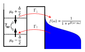
Figure 1: A schematic of an ESR pumped QD system, where a single QD is tunnel coupled to a side electron reservoir characterized by the Fermi function $f(\omega)$, with inverse temperature $\beta=(k_{\rm B}T)^{-1}$ and chemical potential $\mu_{0}$ located in the middle of the spin-up ($\mu_{0}-\frac{\Delta}{2}$) and spin-down ($\mu_{0}+\frac{\Delta}{2}$) levels. The ESR pumping produces a pure spin current in the absence of a net charge current.

We investigate an ESR pumped system closely related to experiments Xiao et al. (2004); Elzerman et al. (2004). The system is comprised of a Coulomb–blockaded single QD, tunnel coupled to a side electron reservoir (Fig. 1). The QD is exposed to a local external rotating magnetic field

$$\bm{B}=\{B_{\parallel}\cos\Omega t,B_{\parallel}\sin\Omega t,B_{\perp}\},$$ (1)

where its $z$ component leads to the Zeeman splitting of the single level $\Delta=g_{\rm z}\mu_{\rm B}B_{\perp}$, with $g_{\rm z}$ the electron $g$-factor in the z direction and $\mu_{\rm B}$ the Bohr magneton. The $x$ and $y$ components of the magnetic field are oscillating in time, where the frequency $\Omega$ is tuned very close to $\Delta$, resulting in the well-known ESR and spin flipping in QD. The electron spin is further tunnel coupled to a side reservoir, whose chemical potential $\mu_{0}$ is set in the middle of the split spin-up and spin-down levels. A spin-up electron may tunnel into QD, where it is pumped to the higher level with its spin orientation flipped and finally tunnels out to the side reservoir. At sufficiently low temperatures, this generates an ESR-pumped spin current without accompanying a net charge current. The Hamiltonian of the total (T) system reads

$$H_{\rm T}(t)=H_{\rm S}(t)+H_{\rm B}+V.$$ (2)

The first term describes the QD with ESR pumping

$$H_{\rm S}(t)= \frac{\Delta}{2}(d^{\dagger}_{\downarrow}d_{\downarrow}-d^{\dagger}_{\uparrow}d_{\uparrow})+U_{\rm C}d^{\dagger}_{\uparrow}d_{\uparrow}d^{\dagger}_{\downarrow}d_{\downarrow}$$

$$+\gamma_{{}_{\rm RF}}(d^{\dagger}_{\uparrow}d_{\downarrow}e^{{\rm i}\Omega t}+d^{\dagger}_{\downarrow}d_{\uparrow}e^{-{\rm i}\Omega t}),$$ (3)

where $d^{\dagger}_{\sigma}$ and $d_{\sigma}$ are the creation and annihilation operators of an electron with spin $\sigma=\{\uparrow,\downarrow\}$ in the QD. Spin-up and spin-down states are coupled to each other due to the rotating magnetic field, with the ESR Rabi frequency given by $\gamma_{{}_{\rm RF}}=g_{\parallel}\mu_{\rm B}B_{\parallel}$ and $g_{\parallel}$ the electron $g$-factor perpendicular to z. We stress that in the following we will consider the Coulomb-blockaded limit $U_{\rm C}\rightarrow\infty$, thus effectively forbidding the double occupancy of the QD.

The second term in Eq. (2) depicts the side electron reservoir, which is modeled as a collection of noninteracting electrons

$$H_{\rm B}=\sum_{\sigma}H_{\rm B}^{(\sigma)}=\sum_{\sigma}\left\{\sum_{k}\varepsilon_{k\sigma}c^{\dagger}_{k\sigma}c_{k\sigma}\right\},$$ (4)

where $H_{\rm B}^{(\sigma)}$ is defined implicitly, with $c^{\dagger}_{k\sigma}$ ($c_{k\sigma}$) the creation (annihilation) operator for an electron with momentum $k$ and spin $\sigma$. For later use, we also introduce the operator for the number of spin-$\sigma$ electrons in the electron reservoir

$$N_{\rm B}^{(\sigma)}=\sum_{k}c^{\dagger}_{k\sigma}c_{k\sigma},$$ (5)

such that the operator for the total number of electrons in the reservoir is $N_{\rm B}=\sum_{\sigma}N_{\rm B}^{(\sigma)}$. The electrode is assumed to be in equilibrium, so that it can be characterized by the Fermi distribution $f(\omega)=\{1+e^{\beta(\omega-\mu_{0})}\}^{-1}$, with the inverse temperature $\beta=(k_{\rm B}T)^{-1}$ and the chemical potential $\mu_{0}$ set in the middle of spin-up and spin-down levels.

The last term in Eq. (2) stands for tunnel coupling between the single QD and side reservoir

$$V=\sum_{\sigma}(f_{\sigma}^{\dagger}d_{\sigma}+d_{\sigma}^{\dagger}f_{\sigma}),$$ (6)

where $f_{\sigma}\equiv\sum_{k}t_{k\sigma}c_{k\sigma}$, with $t_{k\sigma}$ the spin-dependent tunneling amplitude. The corresponding tunneling rate for an electron with spin $\sigma$ is characterized by the intrinsic linewidth $\Gamma_{\sigma}(\omega)=2\pi\sum_{k}|t_{k\sigma}|^{2}\delta(\omega-\varepsilon_{k\sigma})$. Hereafter, we assume wide band limit in the electrodes, which leads to energy independent tunneling rates $\Gamma_{\sigma}(\omega)=\Gamma_{\sigma}$. In what follows, we set unit of $\hbar=e=1$ for the Planck constant and electron charge, unless stated otherwise.

III GQME and Spin Dynamics

In order to describe the energy and particle transport between the QD and side reservoir, we employ the GQME by including corresponding counting fields. Assume the entire system is initially factorized and can be described by the density matrix $\rho_{\rm T}(0)=\rho(0)\otimes\rho_{\rm B}$, where $\rho(0)$ is the density matrix of the reduced system at time $t=0$ and $\rho_{\rm B}$ is that of side reservoir at equilibrium. The generalized density matrix evolves according to Blanter and Büttiker (2000); Nazarov (Ed.)

$$\rho_{\rm T}({\bm{\chi}},t)=\exp_{+}\left\{-{\rm i}\int_{0}^{t}{\rm d}\tau H_{\rm T}({\bm{\chi}},\tau)\right\}\rho_{\rm T}(0)\exp_{-}\left\{{\rm i}\int_{0}^{t}{\rm d}\tau H_{\rm T}(-{\bm{\chi}},\tau)\right\},$$ (7)

where the subscripts $+$ and $-$ stand for time ordering and anti-ordering, respectively. The ${\bm{\chi}}$-dressed Hamiltonian for the entire system in Eq. (7) is given by

$$H_{\rm T}({\bm{\chi}},t)= \exp\left\{\frac{{\rm i}}{2}\sum_{\sigma}(\chi_{1\sigma}N^{(\sigma)}_{\rm B}+\chi_{2\sigma}H_{\rm B}^{(\sigma)})\right\}H_{\rm T}(t)\exp\left\{-\frac{{\rm i}}{2}\sum_{\sigma}(\chi_{1\sigma}N^{(\sigma)}_{\rm B}+\chi_{2\sigma}H_{\rm B}^{(\sigma)})\right\},$$ (8)

where $H_{\rm B}^{(\sigma)}$ and $N^{(\sigma)}_{\rm B}$ are defined in Eqs. (4) and (5), respectively. The involved counting fields read ${\bm{\chi}}=\{\chi_{1\uparrow},\chi_{1\downarrow},\chi_{2\uparrow},\chi_{2\downarrow}\}$, with $\chi_{1\sigma}$ the counting field related to the tunneling of spin $\sigma$ electron, and $\chi_{2\sigma}$ for energy transmission associated with $\sigma$ spin. Since the operators for the QD and reservoir commute, Eq. (8) can be readily expressed as

$$H_{\rm T}({\bm{\chi}},t)=H_{\rm S}(t)+H_{\rm B}+V({\bm{\chi}}),$$ (9)

where $H_{\rm S}(t)$ and $H_{\rm B}$ remain unchanged. It is only the tunnel-coupling Hamiltonian that becomes counting fields dependent

$$V({\bm{\chi}}) =\sum_{\sigma}\{f_{\sigma}({\bm{\chi}})d^{\dagger}_{\sigma}+{\rm h.c.}\},$$ (10)

with $f_{\sigma}({\bm{\chi}})=\sum_{k}t_{k\sigma}c_{k\sigma}e^{-\frac{{\rm i}}{2}(\chi_{1\sigma}+\chi_{2\sigma}\varepsilon_{k\sigma})}$.

If one were given $\rho_{\rm T}({\bm{\chi}},t)$ in Eq. (7), the reduced density matrix in the ${\bm{\chi}}$ space can be readily obtained via $\rho({\bm{\chi}},t)={\rm tr}_{\rm B}\{\rho_{\rm T}({\bm{\chi}},t)\}$, where ${\rm tr}_{\rm B}\{\cdots\}$ represents the trace over the degrees of freedom of reservoir. It leads directly to the cumulant generating function (CGF) in the steady state

$${\cal F}({\bm{\chi}})=\lim_{t\rightarrow\infty}\frac{1}{t}\ln\{{\rm tr}_{\rm S}[\rho({\bm{\chi}},t)]\},$$ (11)

where ${\rm tr}_{\rm S}[\cdots]$ means trace over the degrees of freedom of the reduced system. The statistics of particle and energy currents can be evaluated by simply taking derivatives of the CGF with corresponding counting fields. However, we are neither able to nor interested to track the dynamical evolution of the full system-plus-environment. Instead, we would like to describe the reduced system by a dynamical equation that accounts for (usually approximately) the influence of the environment on the system state, while removing the need to track the full environment evolution.

Figure 2: Stationary occupation of the QD ($\rho^{\rm st}_{11}$) and accumulation of effective spin ($S_{x}^{\rm st}$, $S_{y}^{\rm st}$, $S_{z}^{\rm st}$) versus Rabi frequency for different configurations of asymmetry in spin tunneling. We set $\Gamma=\Gamma_{\uparrow}+\Gamma_{\downarrow}$ as the reference of energy. Other plotting parameters are $\delta=0$, $\Omega/\Gamma=3.0$, $\beta\Gamma=0.1$, and a wide bandwidth ${\rm w}/\Gamma=100$. The inset in Fig. 2(c) shows the $y$-component of the effective magnetic field vs. Rabi frequency.

Here, we assume that the system and reservoir are weakly coupled and perform a second–order perturbation expansion in terms of the coupling Hamiltonian. It is then followed by the conventional Born-Markov approximation but without invoking the widely used secular approximation Hone et al. (2009). To deal with the time-dependent system Hamiltonian, we work in the Floquet basis Shirley (1965); Holthaus and Just (1994); Grifoni and Hänggi (1998); Szczygielski et al. (2013). The GQME finally reads (A detailed derivation is referred to Appendix A)

$$\dot{\rho}({\bm{\chi}},t)=-{\rm i}[H_{\rm S}(t),\rho({\bm{\chi}},t)]+{\cal R}({\bm{\chi}})\rho({\bm{\chi}},t),$$ (12)

where the first term describes the free evolution. The second term stands for dissipation

$${\cal R}({\bm{\chi}})\rho({\bm{\chi}},t)= \bigg{\{}\Gamma_{0,+}({\bm{\chi}}){\cal J}[|u_{0}(t)\rangle\langle u_{+}(t)|]-\frac{1}{2}\Gamma_{0,+}{\cal A}[|u_{0}(t)\rangle\langle u_{+}(t)|]-\frac{{\rm i}}{2}\kappa_{0,+}{\cal C}[|u_{0}(t)\rangle\langle u_{+}(t)|]\bigg{\}}{\rho}({\bm{\chi}},t)$$

$$+\bigg{\{}\Gamma_{0,-}({\bm{\chi}}){\cal J}[|u_{0}(t)\rangle\langle u_{-}(t)|]-\frac{1}{2}\Gamma_{0,-}{\cal A}[|u_{0}(t)\rangle\langle u_{-}(t)|]-\frac{{\rm i}}{2}\kappa_{0,-}{\cal C}[|u_{0}(t)\rangle\langle u_{-}(t)|]\bigg{\}}{\rho}({\bm{\chi}},t)$$

$$+\bigg{\{}\Gamma_{+,0}({\bm{\chi}}){\cal J}[|u_{+}(t)\rangle\langle u_{0}(t)|]-\frac{1}{2}\Gamma_{+,0}{\cal A}[|u_{+}(t)\rangle\langle u_{0}(t)|]-\frac{{\rm i}}{2}\kappa_{+,0}{\cal C}[|u_{+}(t)\rangle\langle u_{0}(t)|]\bigg{\}}{\rho}({\bm{\chi}},t)$$

$$+\bigg{\{}\Gamma_{-,0}({\bm{\chi}}){\cal J}[|u_{-}(t)\rangle\langle u_{0}(t)|]-\frac{1}{2}\Gamma_{-,0}{\cal A}[|u_{-}(t)\rangle\langle u_{0}(t)|]-\frac{{\rm i}}{2}\kappa_{-,0}{\cal C}[|u_{-}(t)\rangle\langle u_{0}(t)|]\bigg{\}}{\rho}({\bm{\chi}},t)$$

$$-\{[\Upsilon_{0,-}+{\rm i}\xi_{0,-}]|u_{+}(t)\rangle\langle u_{-}(t)|{\rho}({\bm{\chi}},t)+[\Upsilon_{0,+}-{\rm i}\xi_{0,+}]{\rho}({\bm{\chi}},t)|u_{+}(t)\rangle\langle u_{-}(t)|\}$$

$$-\{[\Upsilon_{0,+}+{\rm i}\xi_{0,+}]|u_{-}(t)\rangle\langle u_{+}(t)|{\rho}({\bm{\chi}},t)+[\Upsilon_{0,-}-{\rm i}\xi_{0,-}]{\rho}({\bm{\chi}},t)|u_{-}(t)\rangle\langle u_{+}(t)|\}$$

$$+[\Upsilon_{+,0}({\bm{\chi}})+{\rm i}\xi_{+,0}({\bm{\chi}})+\Upsilon_{-,0}({\bm{\chi}})-{\rm i}\xi_{-,0}({\bm{\chi}})]|u_{+}(t)\rangle\langle u_{0}(t)|{\rho}({\bm{\chi}},t)|u_{0}(t)\rangle\langle u_{-}(t)|$$

$$+[\Upsilon_{0,+}({\bm{\chi}})-{\rm i}\xi_{0,+}({\bm{\chi}})+\Upsilon_{0,-}({\bm{\chi}})+{\rm i}\xi_{0,-}({\bm{\chi}})]|u_{0}(t)\rangle\langle u_{-}(t)|{\rho}({\bm{\chi}},t)|u_{+}(t)\rangle\langle u_{0}(t)|$$

$$+[\Upsilon_{+,0}({\bm{\chi}})-{\rm i}\xi_{+,0}({\bm{\chi}})+\Upsilon_{-,0}({\bm{\chi}})+{\rm i}\xi_{-,0}({\bm{\chi}})]|u_{-}(t)\rangle\langle u_{0}(t)|{\rho}({\bm{\chi}},t)|u_{0}(t)\rangle\langle u_{+}(t)|$$

$$+[\Upsilon_{0,+}({\bm{\chi}})+{\rm i}\xi_{0,+}({\bm{\chi}})+\Upsilon_{0,-}({\bm{\chi}})-{\rm i}\xi_{0,-}({\bm{\chi}})]|u_{0}(t)\rangle\langle u_{+}(t)|{\rho}({\bm{\chi}},t)|u_{-}(t)\rangle\langle u_{0}(t)|,$$ (13)

which is expressed in the Floquet basis $|u_{0}(t)\rangle$, $|u_{\pm}(t)\rangle\rangle$ [see Eq. (91)]. The involved superoperators are defined as ${\cal J}[r]\rho=r\rho r^{\dagger}$, ${\cal A}[r]\rho=r^{\dagger}r\rho+\rho r^{\dagger}r$, and ${\cal C}[r]\rho=[r^{\dagger}r,\rho]$. The first four lines describe the tunneling between QD and side reservoir in the Lindblad-like form, with $\Gamma_{0,\pm}$ the rate for an electron in Floquet state $|u_{+}(t)\rangle$ or $|u_{-}(t)\rangle$ to tunnel out of QD, and $\Gamma_{\pm,0}$ for the opposite process. Their connections to the tunneling rates in the original reference $\Gamma^{(\pm)}_{\sigma}$ ($\sigma=\uparrow,\downarrow$) are given by Eqs. (105) and (106). The coefficients $\kappa_{0,\pm}$ and $\kappa_{\pm,0}$ arise purely from the energy renormalization [see Eq. (107)].

The last six lines in Eq. (III) originate from the non-secular treatment. This can be easily verified in Eq. (A), where all these terms are oscillating in the interaction picture. In the case of fast oscillations, the effects of these terms will very quickly average to zero and can thus be neglected. Eq. (III) then reduces to a Lindblad master equation, such that the populations and coherences of the density matrix are dynamically decoupled. In this work, we will go beyond the secular treatment and reveal its essential influence. The involved coefficients $\Upsilon$ and $\xi$, defined in Eqs. (108) and (109), are going to have important roles to play in an effective magnetic field, leading to prominent affects on the energy current.

Investigation of spin dynamics can be achieved by simply propagating Eq. (12) in the limit ${\bm{\chi}}\rightarrow{\bm{0}}$. This can be done, for instance, in the Floquet basis with the diagonal density matrix elements $\rho_{00}(t)=\langle u_{0}(t)|\rho(t)|u_{0}(t)\rangle$, $\rho_{++}(t)=\langle u_{+}(t)|\rho(t)|u_{+}(t)\rangle$, and $\rho_{--}(t)=\langle u_{-}(t)|\rho(t)|u_{-}(t)\rangle$ describing populations, and off-diagonal density matrix elements $\rho_{+-}(t)=\langle u_{+}(t)|\rho(t)|u_{-}(t)\rangle$ and $\rho_{-+}(t)=\langle u_{-}(t)|\rho(t)|u_{+}(t)\rangle$ standing for coherences. Alternatively, in this work we reexpress them in terms of the probabilities and an average spin. We use $\rho_{00}$ and $\rho_{11}=\rho_{++}+\rho_{--}$ to represent the probabilities to find an empty and occupied QD, respectively. We furthermore introduce the vector of average spin ${\bm{S}}=\{S_{x},S_{y},S_{z}\}$, where the individual components are given by

$$S_{x}=\frac{\rho_{+-}+\rho_{-+}}{2},\,S_{y}={\rm i}\frac{\rho_{+-}-\rho_{-+}}{2},\,S_{z}=\frac{\rho_{++}-\rho_{--}}{2}.$$ (14)

Therefore, the dot state is characterized by $\rho({\bm{\chi}})=\{\rho_{00},\rho_{11},S_{x},S_{y},S_{z}\}$. According to GQME (12) and (III), it satisfies

$$\dot{\rho}({\bm{\chi}})={\cal L}({\bm{\chi}})\rho({\bm{\chi}},t),$$ (15)

where ${\cal L}({\bm{\chi}})$ is a $5\times 5$ matrix. Among these five equations, two are for the occupations probabilities and three are for the average spin. The first two read

$$\frac{{\rm d}}{{\rm d}t}\left(\begin{array}[]{c}\rho_{00}\\ \rho_{11}\end{array}\right)= \left(\begin{array}[]{cc}-\Gamma_{+,0}-\Gamma_{-,0}&\frac{1}{2}\{\Gamma_{0,+}({\bm{\chi}})+\Gamma_{0,-}({\bm{\chi}})\}\\ \Gamma_{+,0}({\bm{\chi}})+\Gamma_{-,0}({\bm{\chi}})&-\frac{1}{2}(\Gamma_{0,+}+\Gamma_{0,-})\\ \end{array}\right)\left(\begin{array}[]{c}\rho_{00}\\ \rho_{11}\end{array}\right)$$ (22)

$$+2\left(\begin{array}[]{c}\Upsilon_{0,+}({\bm{\chi}})+\Upsilon_{0,-}({\bm{\chi}})\\ -\Upsilon_{0,+}-\Upsilon_{0,-}\end{array}\right)S_{x}+2\left(\begin{array}[]{c}\xi_{0,+}({\bm{\chi}})-\xi_{0,-}({\bm{\chi}})\\ -\xi_{0,+}+\xi_{0,-}\end{array}\right)S_{y}+\left(\begin{array}[]{c}\Gamma_{0,+}({\bm{\chi}})-\Gamma_{0,-}({\bm{\chi}})\\ -\Gamma_{0,+}+\Gamma_{0,-}\end{array}\right)S_{z}.$$ (29)

Unambiguously, the occupation probabilities are coupled to the spin accumulation in the QD, which is described by the remaining three equations

$$\frac{{\rm d}{\bm{S}}}{{\rm d}t}=\left(\frac{{\rm d}{\bm{S}}}{{\rm d}t}\right)_{\rm acc}+\left(\frac{{\rm d}{\bm{S}}}{{\rm d}t}\right)_{\rm dec}+\left(\frac{{\rm d}{\bm{S}}}{{\rm d}t}\right)_{\rm pre}.$$ (30)

The first term describes the spin accumulation due to tunneling between the electrode and QD

$$\left(\frac{{\rm d}{\bm{S}}}{{\rm d}t}\right)_{\rm acc}\!\!\!\!=\!\!\!\! \left(\!\!\begin{array}[]{cc}\Upsilon_{-,0}({\bm{\chi}})+\Upsilon_{+,0}({\bm{\chi}})&-\frac{1}{2}(\Upsilon_{0,-}\!+\Upsilon_{0,+})\\ \xi_{-,0}({\bm{\chi}})-\xi_{+,0}({\bm{\chi}})&-\frac{1}{2}(\xi_{-,0}-\xi_{+,0})\\ \frac{1}{2}\{\Gamma_{+,0}({\bm{\chi}})-\Gamma_{-,0}({\bm{\chi}})\}&-\frac{1}{2}(\Gamma_{+,0}-\Gamma_{-,0})\\ \end{array}\!\!\right)$$ (34)

$$\cdot\left(\begin{array}[]{c}\rho_{00}\\ \rho_{11}\end{array}\right).$$ (37)

This is the source term responsible for the building up of a spin polarization in the QD. The second term depicts the opposite mechanism – decay of the spin via tunneling out of spin

$$\left(\frac{{\rm d}{\bm{S}}}{{\rm d}t}\right)_{\rm dec}=-\frac{1}{2}(\Gamma_{0,+}+\Gamma_{0,-}){\bm{S}}.$$ (38)

Both spin accumulation and decay depend on the spin orientation, which is described by the third equation

$$\left(\frac{{\rm d}{\bm{S}}}{{\rm d}t}\right)_{\rm pre}={\bm{S}}\times\bm{{\cal B}}.$$ (39)

Interestingly, this term describes the precession of the average spin about an effective magnetic field

$$\bm{{\cal B}} =\{{\cal B}_{x},{\cal B}_{y},{\cal B}_{z}\}$$

$$=\{-(\xi_{0,+}+\xi_{0,-}),(\Upsilon_{0,+}-\Upsilon_{0,-}),\tilde{\epsilon}\},$$ (40)

which arises purely from the non-secular treatment and energy renormalization, with $\tilde{\epsilon}=\epsilon_{-}-\epsilon_{+}+\frac{1}{2}(\kappa_{0,-}-\kappa_{0,+})$. Note that this fictitious magnetic field should not be confused with the real magnetic fields ${\bm{B}}$ in Eq. (1). Later, it will be shown that the subtle interaction between effective magnetic field and spin may have an essential role to play in energy flow through the system.

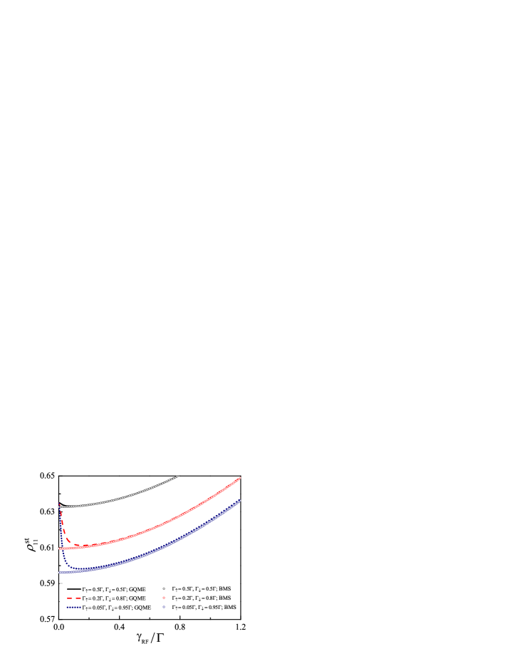
Figure 3: Comparison of stationary occupation in QD ($\rho^{\rm st}_{11}$) using GQME (curves) and BMS master equation (symbols) for various asymmetries in spin tunneling. All other plotting parameters are the same as those in Fig. 2.

In literature, Bloch equation for a pseudospin has also been derived in the singular coupling limit (SCL) Schultz and von Oppen (2009); Breuer and Petruccione (2002); Spohn (1980). By rescaling reservoir Hamiltonian $H_{\rm B}\rightarrow\lambda^{-2}H_{\rm B}$ and tunnel-coupling Hamiltonian $V\rightarrow\lambda^{-1}V$, the reservoir correlation functions experience faster decay and could even be well approximated by $\delta(t)$ in the limit $\lambda\rightarrow 0$. The SCL thus implies a flat spectral density and high temperature limit $k_{\rm B}T\rightarrow\infty$, such that the system energy splitting cannot be resolved. The obtained pseudomagnetic fields arise purely from the energy renormalization Schultz and von Oppen (2009). The GQME employed in this work is obtained under the second order Born-Markov approximation and thus is valid as long as the temperature $k_{\rm B}T\gg\Gamma$. The preservation of positivity is guaranteed by the master equation (III), which has also been checked numerically throughout this work. Furthermore, the effective magnetic field originates not only from the energy renormalization (cf. ${\cal B}_{z}$), but also from the non-secular treatment (see ${\cal B}_{x}$ and ${\cal B}_{y}$), where the latter may have even more important roles to play.

Figure 2 shows the stationary occupation of the QD ($\rho^{\rm st}_{11}$) and effective spin accumulation {$S_{x}^{\rm st}$, $S_{y}^{\rm st}$, $S_{z}^{\rm st}$} versus Rabi frequency for different configurations of asymmetry in spin tunneling. The probability of finding an empty QD ($\rho^{\rm st}_{00}$) is not displayed as it simply satisfies the probability conservation $\rho^{\rm st}_{00}+\rho^{\rm st}_{11}=1$. The occupation of the QD ($\rho^{\rm st}_{11}$) first decreases, reaches a local minimum, and then grows rapidly towards unity with increasing Rabi frequency, cf. Fig. 2(a). In comparison, the results by using a Born-Markov-Secular (BMS) master equation (i.e., by neglecting the last six lines in Eq. (III)) is displayed in Fig. 3. The results using two approaches are consistent in the regime of large Rabi frequencies (not shown explicitly). Yet, noticeable differences are observed for small $\gamma_{{}_{\rm RF}}$, particularly in the case of a large asymmetry in spin tunneling. This is due to the fact that, in the regime of small Rabi frequency, the terms in the last six lines in Eq. (A) do not experience fast oscillation, therefore do not average to zero. Our results show unambiguously that it is not justified to use the secular approximation in the regime of small Rabi frequencies.

In the limit of large Rabi frequency, an electron tunneled into the QD will be almost localized in the Floquet state “$|u_{-}(t)\rangle$” as indicated in $S^{\rm st}_{z}$, cf. Fig. 2(d). The $y$-component of the effective spin decays fast to zero, regardless of the asymmetry in spin tunneling, as shown in Fig. 2(c). It seems to be consistent with the usual secular treatment. However, the $x$-component of the effective spin may survive for a wide range of Rabi frequency, depending on asymmetry in spin tunneling, see Fig. 2(b). We therefore emphasize that the use of a simple BMS master equation may overlook some important dynamics of the reduced system. We will further reveal later that the finite spin accumulation in the QD would have a significant influence on the energy flow through the system.

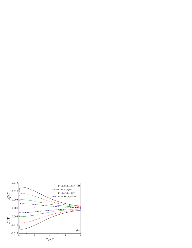
Figure 4: Individual stationary spin currents $J^{\rm st}_{\downarrow}$ and $J^{\rm st}_{\uparrow}$ vs. Rabi frequency for various configurations of spin tunneling asymmetry. All other plotting parameters are the same as those in Fig. 2.

The GQME (12) and (III), or equivalently Eq. (15) enable us to evaluate various currents by employing the CGF

$${\cal F}({\bm{\chi}})=\lim_{t\rightarrow\infty}\frac{1}{t}\ln\{{\rm tr}_{\rm S}[\rho({\bm{\chi}},t)]\}=z_{0}({\bm{\chi}}),$$ (41)

where $z_{0}({\bm{\chi}})$ is the dominant eigenvalue with smallest magnitude of ${\cal L}({\bm{\chi}})$ defined in Eq. (15) and satisfies $z_{0}({\bm{\chi}}\rightarrow{\bm{0}})=0$ Bagrets and Nazarov (2003). The individual stationary spin-$\sigma$ current can be simply obtained as

$$J_{\sigma}^{\rm st}=(-{\rm i})\frac{\partial}{\partial\chi_{1\sigma}}z_{0}({\bm{\chi}})|_{{\bm{\chi}}\rightarrow 0}.$$ (42)

Throughout this work, the superscript “st” is used to represent stationary values. One straightforwardly gets the stationary spin up and spin down currents, respectively, as

$$J_{\uparrow}^{\rm st}= \frac{1}{2}(\Gamma^{(\uparrow)}_{0,+}+\Gamma^{(\uparrow)}_{0,-})\rho^{\rm st}_{11}-[\Gamma^{(\uparrow)}_{+,0}+\Gamma^{(\uparrow)}_{-,0}]\rho^{\rm st}_{00}$$

$$-2[\Upsilon^{(\uparrow)}_{0,+}+\Upsilon^{(\uparrow)}_{0,-}]S^{\rm st}_{x}-2[\xi^{(\uparrow)}_{0,+}-\xi^{(\uparrow)}_{0,-}]S^{\rm st}_{y}$$

$$+(\Gamma^{(\uparrow)}_{0,+}-\Gamma^{(\uparrow)}_{0,-})S^{\rm st}_{z},$$ (43a)

$$J_{\downarrow}^{\rm st}= \frac{1}{2}(\Gamma^{(\downarrow)}_{0,+}+\Gamma^{(\downarrow)}_{0,-})\rho^{\rm st}_{11}-[\Gamma^{(\downarrow)}_{+,0}+\Gamma^{(\downarrow)}_{-,0}]\rho^{\rm st}_{00}$$

$$+2[\Upsilon^{(\downarrow)}_{0,+}+\Upsilon^{(\downarrow)}_{0,-}]S^{\rm st}_{x}+2[\xi^{(\downarrow)}_{0,+}-\xi^{(\downarrow)}_{0,-}]S^{\rm st}_{y}$$

$$+(\Gamma^{(\downarrow)}_{0,+}-\Gamma^{(\downarrow)}_{0,-})S^{\rm st}_{z},$$ (43b)

where $\rho_{jj}^{\rm st}$ ($j=0,1$) and $S^{\rm st}_{\zeta}$ ($\zeta=x,y,z$) are, respectively, the stationary solutions of Eqs. (22) and (30) in the limit ${\bm{\chi}}\rightarrow 0$.

Figure 4 shows the individual spin currents versus Rabi frequency for various configurations of spin tunneling asymmetry. The spin down current ($J_{\downarrow}^{\rm st}$) is positive as it flows out of the QD, while the spin up current ($J_{\uparrow}^{\rm st}$) is negative as it goes into the QD. Whenever an electron tunnels into QD, it will flow out of it. The stationary charge current is thus zero due to charge conservation:

$$J_{\rm ch}^{\rm st}=J^{\rm st}_{\uparrow}+J^{\rm st}_{\downarrow}=0.$$ (44)

This is also confirmed by using Eq. (22). It is worthwhile to mention that this result holds regardless of the degree of asymmetry in spin tunneling.

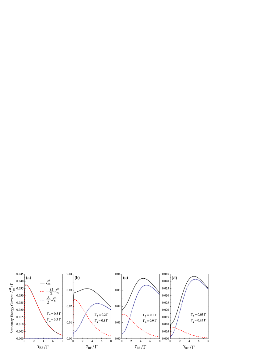
Figure 5: Stationary energy current vs. Rabi frequency for different configurations of spin tunneling asymmetry. For comparison, the contributions from spin current ($-\frac{\Omega}{2}J^{\rm st}_{\rm sp}$) and spin–magnetic field interaction ($\frac{\Lambda}{2}J^{\rm st}_{X}$) are also shown in dashed and dotted curves, respectively. All other plotting parameters are the same as those in Fig. 2.

In the regime of small Rabi frequency, the magnitude of either spin-up or spin-down current increases rapidly with Rabi frequency. In the opposite regime of large Rabi frequency, both fall off gradually towards zero with rising $\gamma_{{}_{\rm RF}}$. This is due to the fact that the electron is inclined to stay in the Floquet state “$|u_{-}(t)\rangle$” as the Rabi frequency increases, cf. Fig. 2(b). A so-called dynamical spin blockade mechanism develops Luo et al. (2015); Ubbelohde et al. (2013); Urban and König (2009); Wang et al. (2011); Luo et al. (2017), which leads eventually to a strong suppression of the current. An increase in spin tunneling asymmetry results in an overall inhibition of both spin-up and spin-down currents. With the knowledge of individual spin currents, one immediately arrives at the net spin current, defined as

$$J_{\rm sp}^{\rm st}\equiv J^{\rm st}_{\uparrow}-J^{\rm st}_{\downarrow}=2J^{\rm st}_{\uparrow},$$ (45)

where we have used the charge conservation, i.e. Eq. (44).

The stationary energy currents, associated with the spin up and spin down currents, can be obtained in an analogous way

$$I_{\sigma}^{\rm st}=(-{\rm i})\frac{\partial}{\partial\chi_{2\sigma}}z_{0}({\bm{\chi}})|_{{\bm{\chi}}\rightarrow 0}.$$ (46)

By utilizing Eq. (15), one immediately arrives at

$$I^{\rm st}_{\uparrow}=(\epsilon_{+}-\epsilon_{0}-\textstyle{\frac{\Omega}{2}}) \left\{\Gamma^{(\uparrow)}_{0,+}\rho^{\rm st}_{++}-\Gamma^{(\uparrow)}_{+,0}\rho^{\rm st}_{00}\right.$$

$$\left.-2\Upsilon^{(\uparrow)}_{0,+}S_{x}^{\rm st}-2\xi^{(\uparrow)}_{0,+}S_{y}^{\rm st}\right\}$$

$$+(\epsilon_{-}-\epsilon_{0}-\textstyle{\frac{\Omega}{2}} )\left\{\Gamma^{(\uparrow)}_{0,-}\rho^{\rm st}_{--}-\Gamma^{(\uparrow)}_{-,0}\rho^{\rm st}_{00}\right.$$

$$\left.-2\Upsilon^{(\uparrow)}_{0,-}S_{x}^{\rm st}+2\xi^{(\uparrow)}_{0,-}S_{y}^{\rm st}\right\},$$ (47a)

$$I^{\rm st}_{\downarrow}=(\epsilon_{+}-\epsilon_{0}+\textstyle{\frac{\Omega}{2}}) \left\{\Gamma^{(\downarrow)}_{0,+}\rho^{\rm st}_{++}-\Gamma^{(\downarrow)}_{+,0}\rho^{\rm st}_{00}\right.$$

$$\left.+2\Upsilon^{(\downarrow)}_{0,+}S_{x}^{\rm st}+2\xi^{(\downarrow)}_{0,+}S_{y}^{\rm st}\right\}$$

$$+(\epsilon_{-}-\epsilon_{0}+\textstyle{\frac{\Omega}{2}} )\left\{\Gamma^{(\downarrow)}_{0,-}\rho^{\rm st}_{--}-\Gamma^{(\downarrow)}_{-,0}\rho^{\rm st}_{00}\right.$$

$$\left.+2\Upsilon^{(\downarrow)}_{0,-}S_{x}^{\rm st}-2\xi^{(\downarrow)}_{0,-}S_{y}^{\rm st}\right\}.$$ (47b)

The total energy current in the steady state is the sum of individual energy currents, and can be readily obtained as

$$I^{\rm st}_{\rm en}=I^{\rm st}_{\uparrow}+I^{\rm st}_{\downarrow}=-\frac{\Omega}{2}J^{\rm st}_{\rm sp}+\frac{\Lambda}{2}J^{\rm st}_{X}.$$ (48)

Unambiguously, it is made up of two components. The first contribution comes from the pure spin current $J^{\rm st}_{\rm sp}$. The second term originates from the interaction between the accumulated spin and the effective magnetic field

$$J^{\rm st}_{X}=4(S^{\rm st}_{x}{\cal B}_{y}-S^{\rm st}_{y}{\cal B}_{x}),$$ (49)

where ${\cal B}_{x}$ and ${\cal B}_{y}$ are respectively the $x$ and $y$ components of the effective magnetic field in Eq. (III). We emphasize that the result in Eq. (48) is of great significance in the following two aspects. First, an energy current can be produced even in the absence of a net matter (charge) current. This is independent of whether the secular approximation is made or not. Second, the interaction between the effective magnetic field and accumulated spin is also responsible for the production of an energy current. This contribution purely originates from the non-secular treatment. It will be revealed that this term may have essential roles to play in the energy flow under the circumstance of strongly asymmetric spin tunneling rates.

In Fig. 5 the stationary energy current ($I_{\rm en}^{\rm st}$) is plotted against Rabi frequency ($\gamma_{{}_{\rm RF}}$) for various configurations of spin tunneling asymmetry. The contributions due to spin current and spin accumulation are also exhibited by the dashed and dotted curves, respectively. In the case of symmetric spin tunneling ($\Gamma_{\uparrow}=\Gamma_{\downarrow}=0.5\Gamma$), the spin accumulation ($J^{\rm st}_{X}$) has a negligible contribution and the energy current is dominated by the spin current ($J^{\rm st}_{\rm sp}$), cf. Fig. 5(a). The behavior of the total energy current is thus similar to the spin current in Fig. 4, i.e., it first increases rapidly with rising Rabi frequency, reaches a maximum at approximately $\gamma_{{}_{\rm RF}}\approx 0.5\Gamma$, and finally falls off and approaches zero in the limit $\gamma_{{}_{\rm RF}}\rightarrow\infty$.

The picture becomes drastically different under the circumstance of strong asymmetry in spin tunneling, where the spin current is suppressed while the contribution from interaction between effective magnetic field and spin accumulation has an essential role to play. For instance, a strong asymmetry of $\Gamma_{\uparrow}=0.2\Gamma$ and $\Gamma_{\downarrow}=0.8\Gamma$ gives rise to a prominent enhancement in $\frac{\Lambda}{2}J^{\rm st}_{X}$ at approximately $\gamma_{{}_{\rm RF}}\approx 5\Gamma$. This is ascribed to noticeable effective magnetic field ${\cal B}_{y}$ [inset of Fig. 2(b)] and finite spin accumulation $S^{\rm st}_{x}$ [Fig. 2(b)] ($S^{\rm st}_{y}$ has a vanishing contribution, cf. Fig. 2(c)). It leads to the emergence of a local maximum in the energy current at $\gamma_{{}_{\rm RF}}\approx 3\Gamma$, in addition to its original maximum at $\gamma_{{}_{\rm RF}}\approx 0.5\Gamma$, see Fig. 5(b). Remarkably, for an extremely asymmetric tunneling rates ($\Gamma_{\uparrow}=0.05\Gamma,\Gamma_{\downarrow}=0.95\Gamma$) as shown in Fig. 5(d), the $J^{\rm st}_{X}$-term serves as the dominant contribution. As a result, one observes solely a single maximum in energy current at $\gamma_{{}_{\rm RF}}\approx 5\Gamma$. Our results show unambiguously the importance of considering the interaction between effective magnetic field and spin accumulation for very asymmetric spin tunneling rates. In this case, the use of a simple BMS master equation picture would be fundamentally insufficient.

IV Stochastic Thermodynamics

Now we are in a position to discuss the stochastic thermodynamics, i.e., the identification of the first and second laws at the microscopic level. Our analysis is based on the two-measurement process theory and the method of counting statistics Esposito et al. (2009). We will focus on energy and entropy balance of the ESR pumped QD system in the steady-state limit.

IV.1 Energy balance based on statistics of
work and heat

In this subsection we characterize the steady fluctuations of work and heat by evaluating their counting statistics using initial and final measurements of the system energy. Statistics of work has previously been analyzed with quantum jump approach Hekking and Pekola (2013) or Lindblad quantum master equations Silaev et al. (2014). Here we employ the two-measurement process approach Esposito et al. (2009); Solinas et al. (2013) within the framework of the GQME, thus fully accounting for effect of the non-secular treatment and the coherences.

Let us denote the instantaneous eigenenergies of $H_{\rm S}(t)$ as $e_{m}(t)$ and those of $H_{\rm B}$ as $\varepsilon_{k}$. Assume that at time $t=0$ a joint measurement of $H_{\rm S}(0)$ and $H_{\rm B}$ is performed, yielding the outcomes $e_{m}(0)$ and $\varepsilon_{k}$, respectively. At time $t>0$, a second joint measurement of $H_{\rm S}(t)$ and $H_{\rm B}$ is made with outcomes $e_{n}(t)$ and $\varepsilon_{k^{\prime}}$. The energy changes of system and bath, $\Delta e$ and $\Delta\varepsilon$, respectively, in a single realization of the protocol are thus given by

$$\Delta e =e_{n}(t)-e_{m}(0),$$ (50a)

$$\Delta\varepsilon =\varepsilon_{k^{\prime}}-\varepsilon_{k}.$$ (50b)

The change of the energy of the entire system is given by the sum of the energy changes of the reduced system and bath energies, apart from a negligible contribution due to the system-bath interaction. The work $W$ performed on the system coincides with the change of the energy of the entire system because the driving is acted solely onto the reduced system, i.e.,

$$W=\Delta e+\Delta\varepsilon=e_{n}(t)+\varepsilon_{k^{\prime}}-e_{m}(0)-\varepsilon_{k}.$$ (51)

Apparently, $W$ is a random variable due to the intrinsic randomness in the quantum measurement processes. The statistical properties of $W$ can be conveniently expressed in terms of its characteristic function

$$G_{W}(\chi_{W},t)=\int_{-\infty}^{\infty}{\rm d}We^{{\rm i}W\chi_{W}}P(W,t),$$ (52)

where $P(W,t)$ is probability density function of observing an amount of work $W$ performed by the external driving from time 0 to $t$, and $\chi_{W}$ is the corresponding counting field. According to the theory of two-measurement process Esposito et al. (2009), the probability density function is given by

$$P(W,t)\!= \!\!\sum_{e_{n}(t),e_{m}(0)}\sum_{\varepsilon_{k},\varepsilon_{k^{\prime}}}\!\delta[e_{n}(t)\!+\varepsilon_{k^{\prime}}\!-e_{m}(0)-\varepsilon_{k}-W]$$

$$\cdot p(e_{n}(t)\!+\varepsilon_{k^{\prime}}|e_{m}(0)\!+\varepsilon_{k})p(e_{m}(0)\!+\varepsilon_{k}),$$ (53)

where $p(e_{n}(t)+\varepsilon_{k^{\prime}}|e_{m}(0)+\varepsilon_{k})$ is the conditional probability that a measurement of $H_{\rm S}(t)$ and $H_{\rm B}$ gives $e_{n}(t)$ and $\varepsilon_{k^{\prime}}$, respectively, at time $t$ given that it gave $e_{m}(0)$ and $\varepsilon_{k}$ at time 0, while $p(e_{m}(0)+\varepsilon_{k})$ is the usual probability to have $e_{m}(0)$ and $\varepsilon_{k}$ at time 0.

By introducing the projectors $\hat{\cal P}_{e_{j}(t)}$ and $\hat{\cal P}_{\varepsilon_{k}}$ on the $j$-th state of the system with energy $e_{j}(t)$ and $k$-th state of the reservoir with energy $\varepsilon_{k}$, one has

$$p(e_{n}(t)+\varepsilon_{k^{\prime}}|e_{m}(0)+\varepsilon_{k})p(e_{m}(0)+\varepsilon_{k})$$

$$={\rm tr}[\hat{\cal P}_{e_{n}(t)}\hat{\cal P}_{\varepsilon_{k^{\prime}}}U(t)\hat{\cal P}_{e_{m}(0)}\hat{\cal P}_{\varepsilon_{k}}\rho_{\rm T}(0)$$

$$\hskip 21.52771pt\times\hat{\cal P}_{\varepsilon_{k}}\hat{\cal P}_{e_{m}(0)}U^{\dagger}(t)\hat{\cal P}_{\varepsilon_{k^{\prime}}}\hat{\cal P}_{e_{n}(t)}],$$ (54)

where ${\rm tr}[\cdots]$ represents the trace over the degrees of the freedom of entire system, and $U(t)$ is the evolution operator associated with the entire Hamiltonian $H_{\rm T}(t)$:

$$U(t)=\exp_{+}\left(-{\rm i}\int_{0}^{t}{\rm d}\tau H_{\rm T}(\tau)\right).$$ (55)

Next we assume that the initial total density matrix can be factorized to $\rho_{\rm T}(0)=\frac{e^{-\beta H_{\rm S}(0)}}{Z_{\rm S}(0)}\otimes\frac{e^{-\beta H_{\rm B}}}{Z_{\rm B}}$, where $Z_{\rm S}(0)={\rm tr}_{\rm S}\{e^{-\beta H_{\rm S}(0)}\}$ is the partition function of system at time $t=0$ and $Z_{\rm B}={\rm tr}_{\rm B}\{e^{-\beta H_{\rm B}}\}$ is that of reservoir. By using $\hat{\cal P}^{2}_{e_{j}(t)}=\hat{\cal P}_{e_{j}(t)}$ and $\hat{\cal P}^{2}_{\varepsilon_{k}}=\hat{\cal P}_{\varepsilon_{k}}$, Eq. (IV.1) is further simplified to

$$p(e_{n}(t)+\varepsilon_{k^{\prime}}|e_{m}(0)+\varepsilon_{k})p(e_{m}(0)+\varepsilon_{k})$$

$$={\rm tr}[U^{\dagger}(t)\hat{\cal P}_{e_{n}(t)}\hat{\cal P}_{\varepsilon_{k^{\prime}}}U(t)\hat{\cal P}_{e_{m}(0)}\hat{\cal P}_{\varepsilon_{k}}\rho_{\rm T}(0)].$$ (56)

Noticing that $\sum_{e_{j}(t)}\hat{{\cal P}}_{e_{j}(t)}e^{\pm{\rm i}\chi_{W}e_{j}(t)}=e^{\pm{\rm i}\chi_{W}H_{\rm S}(t)}$ and $\sum_{\varepsilon_{k}}\hat{{\cal P}}_{\varepsilon_{k}}e^{\pm{\rm i}\chi_{W}\varepsilon_{k}}=e^{\pm{\rm i}\chi_{W}H_{\rm B}}$, the characteristic function of work in Eq. (52) can be written as

$${G}_{W}(\chi_{W},\!t)\!= {\rm tr}\!\left\{\!e^{{\rm i}\frac{\!\chi_{W}}{2}[H_{\rm S}(t)+H_{\rm B}]}U(t)e^{-{\rm i}\frac{\!\chi_{W}}{2}[H_{\rm S}(0)+H_{\rm B}]}\!\rho_{\rm T}(0)\right.$$

$$\;\;\;\cdot\left.e^{-{\rm i}\frac{\chi_{W}}{2}[H_{\rm S}(0)+H_{\rm B}]}U^{\dagger}(t)e^{{\rm i}\frac{\chi_{W}}{2}[H_{\rm S}(t)+H_{\rm B}]}\right\},$$

$$= \sum_{e_{n}(t),e_{m}(0)}\frac{e^{{\rm i}\chi_{W}[e_{n}(t)-e_{m}(0)]-\beta e_{m}(0)}}{Z_{\rm S}(0)}$$

$$\;\;\;\cdot\langle e_{n}(t)|\varrho(\chi_{W},t;e_{m}(0))|e_{n}(t)\rangle,$$ (57)

where we have introduced a new density matrix of the reduced system including the counting field of work

$$\varrho(\chi_{W},t;e_{m}(0))= {\rm tr}_{\rm B}\left\{e^{{\rm i}\frac{\chi_{W}}{2}H_{\rm B}}U(t)e^{-{\rm i}\frac{\chi_{W}}{2}H_{\rm B}}\varrho(0;e_{m}(0))\right.$$

$$\hskip 12.91663pt\left.\otimes\,\rho_{\rm B}\,e^{-{\rm i}\frac{\chi_{W}}{2}H_{\rm B}}U^{\dagger}(t)e^{{\rm i}\frac{\chi_{W}}{2}H_{\rm B}}\right\}.$$ (58)

By comparing with Eqs. (7) and (8), one finds that $\varrho(\chi_{W},t;e_{m}(0))$ satisfies the same equation as $\rho({\bm{\chi}},t)$ does, i.e. Eq. (15), with only the crucial replacement

$$\varrho(\chi_{W},t;e_{m}(0))=\rho({\bm{\chi}},t)|_{\chi_{1\uparrow}=\chi_{1\downarrow}=0,\chi_{2\uparrow}=\chi_{2\downarrow}=\chi_{W}}$$ (59)

and initial condition $\varrho(0;e_{m}(0))=|e_{m}(0)\rangle\langle e_{m}(0)|$. Unambiguously, both populations and coherences have important roles to play in the statistics of work. Here, we are interested in the stationary statistics, therefore, the CGF of the mechanical power is simply given by

$${\cal G}_{W}(\chi_{W},t)= \lim_{t\rightarrow\infty}\frac{1}{t}\ln G_{W}(\chi_{W},t)$$

$$= z_{0}({\bm{\chi}})|_{\chi_{1\uparrow}=\chi_{1\downarrow}=0,\chi_{2\uparrow}=\chi_{2\downarrow}=\chi_{W}},$$ (60)

where $z_{0}({\bm{\chi}})$ is the dominant eigenvalue with smallest magnitude of ${\cal L}({\bm{\chi}})$ as shown in Eq. (41).

The average rate of mechanical work is simply obtained

$$\dot{W} =-{\rm i}\frac{\partial}{\partial\chi_{W}}z_{0}(\{0,0,\chi_{W},\chi_{W}\})|_{\chi_{W}\rightarrow 0}$$

$$=I_{\uparrow}^{\rm st}+I_{\downarrow}^{\rm st}=-\frac{\Omega}{2}J^{\rm st}_{\rm sp}+\frac{\Lambda}{2}J^{\rm st}_{X}.$$ (61)

It shows clearly that the work done on the system is used to produce a spin current and a precession of an average spin in the QD, where the latter originates purely from non-secular treatment.

The statistical properties of the heat flow can be analyzed in a similar way by using the two-measurement process theory Esposito et al. (2009); Gasparinetti et al. (2014). Assume at time $t=0$ a measurement $H_{\rm B}$ yields an outcome $\varepsilon_{k}$. A little later at $t>0$, a second measurement is made with outcome $\varepsilon_{k^{\prime}}$. The heat flows from the reservoir to the QD is given by

$$Q=-(\varepsilon_{k^{\prime}}-\varepsilon_{k}).$$ (62)

Analogously to Eq. (52), the characteristic function of heat flow is defined as

$$G_{Q}(\chi_{Q},t)=\int_{-\infty}^{\infty}{\rm d}Qe^{{\rm i}Q\chi_{Q}}P(Q,t),$$ (63)

where $\chi_{Q}$ is the counting field associated with heat flow, and $P(Q,t)$ is the probability density function of observing an amount of heat $Q$ flowed in to QD from time 0 to $t$. It can be determined from the two-time measurement approach Esposito et al. (2009):

$$P(Q,t)=\sum_{\varepsilon_{k},\varepsilon_{k^{\prime}}}\delta[\varepsilon_{k^{\prime}}-\varepsilon_{k}+Q)]p(\varepsilon_{k^{\prime}}|\varepsilon_{k})p(\varepsilon_{k}),$$ (64)

where $p(\varepsilon_{k^{\prime}}|\varepsilon_{k})$ is the conditional probability for observing $\varepsilon_{k^{\prime}}$ at time $t$, given that it yields $\varepsilon_{k}$ at time 0, while $p(\varepsilon_{k})$ is the usual probability to have $\varepsilon_{k}$ at time 0. By following similar procedures in Eqs. (IV.1) and (IV.1), the characteristic function of heat flow can be expressed as

$${G}_{Q}(\chi_{Q},t)={\rm tr}_{\rm S}[\varrho(-\chi_{Q},t)],$$ (65)

where $\varrho(-\chi_{Q},t)$ satisfies the same equation as $\rho({\bm{\chi}},t)$ in Eq. (15), with only the replacement $\varrho(-\chi_{Q},t)=\rho({\bm{\chi}},t)|_{\chi_{1\uparrow}=\chi_{1\downarrow}=0,\chi_{2\uparrow}=\chi_{2\downarrow}=-\chi_{Q}}$. In comparison with the Eq. (41), one immediately finds the CGF of the heat flow in the stationary limit

$${\cal G}_{Q}(\chi_{Q}) =\lim_{t\rightarrow\infty}\frac{1}{t}\ln G_{Q}(\chi_{Q},t)$$

$$=z_{0}({\bm{\chi}})_{\chi_{1\uparrow}=\chi_{1\downarrow}=0,\chi_{2\uparrow}=\chi_{2\downarrow}=-\chi_{Q}},$$ (66)

where $z_{0}({\bm{\chi}})$ is the dominant eigenvalue with smallest magnitude of ${\cal L}({\bm{\chi}})$ in Eq. (41). The average heat flowing into QD is simply given by

$$\dot{Q} =-{\rm i}\frac{\partial}{\partial\chi_{Q}}z_{0}(\{0,0,-\chi_{Q},-\chi_{Q}\})|_{\chi_{Q}\rightarrow 0}$$

$$=-(I_{\uparrow}^{\rm st}+I_{\downarrow}^{\rm st}).$$ (67)

By comparing with Eqs. (IV.1), one eventually arrives at the energy balance relation in terms of the first law of thermodynamics

$$\dot{E}=\dot{Q}+\dot{W}=0.$$ (68)

The work done on the system is completely converted into heat, such that the net increase of energy in the QD is zero in the stationary limit.

IV.2 Entropy balance

We are now in a position to investigate the entropy balance and identify the second law on the microscopic level. For a system described by a Lindblad master equation, it has been shown that a connection between entropy production and the heat currents can be established based on the local detailed balance (LDB) relation Esposito and Van den Broeck (2010). A similar LDB was found in a driven system under secular approximation, where the populations and coherences are dynamically decoupled Silaev et al. (2014); Cuetara et al. (2015). Our analysis is based on the GQME beyond the secular approximation such that both populations and coherences have vital roles to play. We will establish the connection between entropy production and heat flow in the stationary limit, using the two-measurement process theory and the method of counting statistics, rather than the LDB.

We start with the von Neumann entropy

$$S(t)=-{\rm tr}_{\rm S}[\rho(t)\ln\rho(t)],$$ (69)

where $\rho(t)$ is the density matrix of the reduced system. The change in von Neumann entropy $\Delta S$ can be decomposed into an entropy production $\Delta S_{\rm i}$ and an entropy flow $\Delta S_{\rm e}$ Kondepudi and Prigogine (1998); de Groot and Mazur (1984); Prigogine and Nicolis (1977); Gaspard (2006), where the latter is given by the heat exchanged with the reservoir multiplied by the inverse temperature

$$\Delta S_{\rm e}=\beta\Delta Q.$$ (70)

The entropy production then is given by

$$\Delta S_{\rm i}=\Delta S-\beta\Delta Q.$$ (71)

In what follows, we will analyze the entropy from a statistical point of view, using the two-measurement process analogous to that in Eq. (IV.1). Assume at time $t=0$, joint measurements of the energies of system and reservoir are made. The obtained energy eigenvalues are denoted by $e_{m}(0)$ and $\epsilon_{k}$, respectively. The associated von Neumann entropy of the system is ${S}(0)=\beta[e_{m}(0)-{F}_{0}]$, where ${F}_{0}=-\frac{1}{\beta}\ln{Z}_{0}$ is the free energy with $\ln{Z}_{0}=-\ln p(e_{m}(0))-\beta e_{m}(0)$. Later at time $t$, a similar joint measurement yields $e_{n}(t)$ and $\epsilon_{k^{\prime}}$, respectively. The corresponding entropy thus is ${S}(t)=\beta[e_{n}(t)-{F}_{t}]$, with free energy ${F}_{t}=-\frac{1}{\beta}\ln{Z}_{t}$ and $\ln{Z}_{t}=-\ln p(e_{n}(t))-\beta e_{n}(t)$. The change in entropy is

$$\Delta S=S(t)-S(0)=\ln p(e_{m}(0))-\ln p(e_{n}(t)).$$ (72)

Apparently, $\Delta S$ is a random variable owing to the stochastic nature in the quantum measurement. Its probability density function is given by

$$P(\Delta S,t)= \!\!\!\!\sum_{e_{n}(t),e_{m}(0)}\sum_{\varepsilon_{k},\varepsilon_{k^{\prime}}}\!\!\delta[\ln p(e_{m}(0))\!-\ln p(e_{n}(t))\!-\!\Delta S]$$

$$\cdot p(e_{n}(t)+\varepsilon_{k^{\prime}}|e_{m}(0)+\varepsilon_{k})p(e_{m}(0)+\varepsilon_{k}),$$ (73)

where we have used the same probabilities $p(e_{n}(t)+\varepsilon_{k^{\prime}}|e_{m}(0)+\varepsilon_{k})$ and $p(e_{m}(0)+\varepsilon_{k})$ as in Eq. (IV.1). In a single realization the entropy can be expressed as

$$\Delta S=\Delta S_{\rm i}+\beta\Delta Q,$$ (74)

where $\Delta Q=-(\varepsilon_{k^{\prime}}-\varepsilon_{k})$ is the heat flowed into the QD. One finds the probability density function for entropy production:

$$P(\Delta S_{\rm i},t)= \sum_{e_{n}(t),e_{m}(0)}\sum_{\varepsilon_{k},\varepsilon_{k^{\prime}}}\delta[\ln p(e_{m}(0))-\ln p(e_{n}(t))$$

$$\hskip 71.13188pt-\Delta S_{\rm i}+\beta(\varepsilon_{k^{\prime}}-\varepsilon_{k})]$$

$$\cdot p(e_{n}(t)+\varepsilon_{k^{\prime}}|e_{m}(0)+\varepsilon_{k})p(e_{m}(0)+\varepsilon_{k}).$$ (75)

Its corresponding characteristic function can be obtained by simply performing a Fourier transform

$$G_{\Delta S_{\rm i}}(\chi_{S_{i}}) =\int_{-\infty}^{\infty}{\rm d}(\Delta S_{\rm i})P(\Delta S_{\rm i},t)\,e^{{\rm i}\Delta S_{\rm i}\chi_{S_{i}}},$$ (76)

where $\chi_{S_{i}}$ is the counting field associated with the entropy production. In parallel to the discussion for the statistics of work, it can be expressed as

$$G_{\Delta S_{\rm i}}(\chi_{S_{i}},t)= \!\!\!\sum_{e_{n}(t),e_{m}(0)}\!\!\!\frac{e^{{\rm i}\chi_{S_{i}}[\ln p(e_{m}(0))-\ln p(e_{n}(t))]-\beta e_{m}(0)}}{Z_{\rm S}(0)}$$

$$\;\;\;\;\;\;\cdot\langle e_{n}(t)|\varrho(\chi_{S_{i}}\beta,t;e_{m}(0))|e_{n}(t)\rangle,$$ (77)

where $\varrho(\chi_{S_{i}}\beta,t;e_{m}(0))$ satisfies the same equation as $\rho({\bm{\chi}},t)$ in Eq. (15), with only the replacement $\varrho(\chi_{S_{i}}\beta,t;e_{m}(0))=\rho({\bm{\chi}},t)|_{\chi_{1\uparrow}=\chi_{1\downarrow}=0,\chi_{2\uparrow}=\chi_{2\downarrow}=\chi_{S_{i}}\beta}$ and initial condition $\varrho(0;e_{m}(0))=|e_{m}(0)\rangle\langle e_{m}(0)|$.

The CGF for the entropy production characterizing the stationary statistics is thus given by

$${\cal G}_{S_{\rm i}}(\chi_{S_{i}})= \lim_{t\rightarrow\infty}\frac{1}{t}\ln G_{\Delta S_{\rm i}}(\chi_{S_{i}},t)$$

$$= z_{0}({\bm{\chi}})|_{\chi_{1\uparrow}=\chi_{1\downarrow}=0,\chi_{2\uparrow}=\chi_{2\downarrow}=\chi_{S_{i}}\beta},$$ (78)

where $z_{0}({\bm{\chi}})$ is the dominant eigenvalue with smallest magnitude of ${\cal L}({\bm{\chi}})$, as shown in Eq. (41). The average irreversible entropy production then is simply obtained by taking partial derivative of ${\cal G}_{S_{\rm i}}(\chi_{S_{i}})$

$$\dot{S_{\rm i}} =-{\rm i}\frac{\partial}{\partial\chi_{S_{i}}}z_{0}(\{0,0,\chi_{S_{i}}\beta,\chi_{S_{i}}\beta\})|_{\chi_{S_{i}}\rightarrow 0}$$

$$=\beta(I_{\uparrow}^{\rm st}+I_{\downarrow}^{\rm st})=\beta I_{\rm en}^{\rm st}\geq 0.$$ (79)

This is the second law formulated as the non-negativity of the irreversible entropy production, owing to the non-negative energy current that we have confirmed numerically, see also Fig. 5. Furthermore, it means that both populations and coherences of the density matrix have essential roles to play in entropy production. By recalling Eq. (IV.1) and the energy balance relation Eq. (68), one finds

$$\dot{S}_{\rm i}=-\beta\dot{Q}=\frac{\beta}{2}(-\Omega J_{\rm sp}^{\rm st}+\Lambda J_{X}^{\rm st}).$$ (80)

The first equality manifests the relation between entropy production and heat current based on counting statistics, rather than the LDB. Together with the entropy flow defined in Eq. (70), one arrives at the entropy balance in the stationary limit

$$\dot{S}=\dot{S}_{\rm i}+\dot{S}_{\rm e}=0.$$ (81)

The second equality in Eq. (80), to the best of our knowledge, is a new result, revealing not only its relation to a pure spin current, but also the intimate connection to the influence of interaction between effective spin and effective magnetic field. Finally, we remark that the contribution from $J_{X}^{\rm st}$ is of the first order in tunnel-coupling strength, and thus could be detected in experiment. We highly anticipate this to be verified in the near future.

V Conclusion

In summary, we have performed a stochastic thermodynamics analysis of an ESR pumped quantum dot system in the presence of a pure spin current only. The state of the system can be described by populations and an effective spin in the Floquet basis. In particular, this effective spin undergoes a precession about an effective magnetic field, which originates from the non-secular treatment and energy renormalization. Unambiguously, an energy current could be generated, not due to a charge current, but entailed by a pure spin current and the interaction between effective spin and effective magnetic field, where the latter may have the dominant role to play in the case of strong asymmetry in spin tunneling. In the stationary limit, energy balance and entropy balance relations are established based on the theory of counting statistics. Furthermore, we revealed a new mechanism that the irreversible entropy production is found to be intimately related to the interaction between effective spin and magnetic field.

Appendix A Derivation of the GQME

First, we transform from the Schrödinger’s picture to the interaction picture

$$\tilde{\rho}_{\rm T}({\bm{\chi}},t)=U^{\dagger}_{0}(t)\rho_{\rm T}({\bm{\chi}},t)U_{0}(t),$$ (82)

where

$$U_{0}(t)\equiv\exp_{+}\left\{-{\rm i}\int_{0}^{t}{\rm d}\tau H_{\rm S}(\tau)\right\}e^{-{\rm i}H_{\rm B}t}.$$ (83)

In what follows, the tilde is used to indicate a quantity in the interaction picture. The equation of motion of $\tilde{\rho}_{\rm T}({\bm{\chi}},t)$ then reads

$$\frac{{\rm d}}{{\rm d}t}{\tilde{\rho}}_{\rm T}({\bm{\chi}},t)=-{\rm i}\{\tilde{V}({\bm{\chi}},t)\tilde{\rho}_{\rm T}({\bm{\chi}},t)-\tilde{\rho}_{\rm T}({\bm{\chi}},t)\tilde{V}(-{\bm{\chi}},t)\},$$ (84)

with

$$\tilde{V}({\bm{\chi}},t)=U_{0}^{\dagger}(t)V({\bm{\chi}})U_{0}(t).$$ (85)

Now, we integrate Eq. (84) twice, differentiate with respect to time “$t$”, and trace over the degrees of freedom of the reservoir. This yields an exact equation of motion for the ${\bm{\chi}}$-dependent reduced density matrix

$$\frac{{\rm d}}{{\rm d}t}{\tilde{\rho}}({\bm{\chi}},t)=-\int_{0}^{t} {\rm d}\tau\,{\rm tr}_{\rm B}\{\tilde{V}({\bm{\chi}},t)\tilde{V}({\bm{\chi}},\tau)\tilde{\rho}_{\rm T}({\bm{\chi}},\tau)$$

$$-\tilde{V}({\bm{\chi}},\tau)\tilde{\rho}_{\rm T}({\bm{\chi}},\tau)\tilde{V}(-{\bm{\chi}},t)$$

$$-\tilde{V}({\bm{\chi}},t)\tilde{\rho}_{\rm T}({\bm{\chi}},\tau)\tilde{V}(-{\bm{\chi}},\tau)$$

$$+\tilde{\rho}_{\rm T}({\bm{\chi}},\tau)\tilde{V}(-{\bm{\chi}},\tau)\tilde{V}(-{\bm{\chi}},t)\},$$ (86)

where ${\rm tr}_{\rm B}\{\cdots\}$ stands for the trace over the degrees of freedom of reservoir. This equation still contains the density matrix $\tilde{\rho}_{\rm T}({\bm{\chi}},\tau)$ of the entire system. We thus now make the Born approximation which assumes that the density operator factorises at all times as $\tilde{\rho}_{\rm T}({\bm{\chi}},\tau)=\tilde{\rho}({\bm{\chi}},\tau)\otimes\rho_{\rm B}$. It greatly simplifies Eq. (A). Yet, it still has a time non-local form: The future evolution ${\tilde{\rho}}({\bm{\chi}},t)$ depends on its past history ${\tilde{\rho}}({\bm{\chi}},\tau)$, which makes it difficult to work with. In case of a large separation between system and environment timescales, it is justified to introduce the Markov approximation, i.e., replacing $\tilde{\rho}({\bm{\chi}},\tau)$ by $\tilde{\rho}({\bm{\chi}},t)$ and extending the upper limit of the integral to infinity in Eq. (A). Finally, it yields a closed differential equation of motion for the reduced density matrix that the future behaviour of ${\tilde{\rho}}({\bm{\chi}},t)$ depends only on its present state

$$\frac{{\rm d}}{{\rm d}t}{\tilde{\rho}}({\bm{\chi}},t)= -\!\int_{0}^{\infty}\!{\rm d}\tau{\rm tr}_{\rm B}\{\tilde{V}({\bm{\chi}},t)\tilde{V}({\bm{\chi}},t-\tau)\rho_{\rm B}\!\otimes\tilde{\rho}({\bm{\chi}},t)$$

$$-\tilde{V}({\bm{\chi}},t-\tau)\rho_{\rm B}\!\otimes\tilde{\rho}({\bm{\chi}},t)\tilde{V}(-{\bm{\chi}},t)$$

$$-\tilde{V}({\bm{\chi}},t)\rho_{\rm B}\!\otimes\tilde{\rho}({\bm{\chi}},t)\tilde{V}(-{\bm{\chi}},t-\tau)$$

$$+\rho_{{\rm B}}\!\otimes\tilde{\rho}({\bm{\chi}},t)\tilde{V}(-{\bm{\chi}},t-\tau)\tilde{V}(-{\bm{\chi}},t)\}$$

$$= -\{{\rm[I]}-{\rm[II]}-{\rm[III]}+{\rm[IV]}\}.$$ (87)

This serves as an essential starting point for the following derivation.

Each term in Eq. (A) has to be evaluated, which requires the explicit form of the $V({\bm{\chi}},t)$ in Eq. (85). By utilizing Eqs. (10) and (83), one immediately has

$$\tilde{f}_{\sigma}({\bm{\chi}},t)= U^{\dagger}_{0}(t){f}_{\sigma}({\bm{\chi}})U_{0}(t)$$

$$= \sum_{k}t_{k\sigma}c_{k\sigma}e^{-\frac{{\rm i}}{2}(\chi_{2\sigma}\varepsilon_{k\sigma}+\chi_{1\sigma})}e^{-{\rm i}\varepsilon_{k\sigma}t}.$$ (88)

The system operators in the interaction picture are defined analogously

$$\tilde{d}_{\sigma}(t) =U^{\dagger}_{0}(t){d}_{\sigma}(t)U_{0}(t)$$

$$=\exp_{-}\left\{{\rm i}\int_{0}^{t}H_{\rm S}(\tau)d\tau\right\}d_{\sigma}\exp_{+}\left\{-{\rm i}\int_{0}^{t}H_{\rm S}(\tau)d\tau\right\},$$ (89)

where the time ordering arises purely from the time dependence of the system Hamiltonian. To explicitly evaluate Eq. (A), we employ Floquet theory Shirley (1965); Holthaus and Just (1994); Grifoni and Hänggi (1998); Szczygielski et al. (2013), which states that the unitary evolution can be represented as

$$\exp_{+}\left\{\!-{\rm i}\int_{0}^{t}H_{\rm S}(\tau)d\tau\right\}=\sum_{j}e^{-{\rm i}\epsilon_{j}t}|u_{j}(t)\rangle\langle u_{j}(0)|,$$ (90)

where $|u_{j}(t)\rangle$ is the Floquet function inherits the periodicity $|u_{j}(t)\rangle=|u_{j}(t+T)\rangle$ with $T=\frac{2\pi}{\Omega}$, and $\epsilon_{j}$ is the corresponding quasienergy. The quasienergies and Floquet functions are simply given, respectively, by

$$\epsilon_{0} =0,\hskip 31.2982pt|u_{0}(t)\rangle=\left(\begin{array}[]{c}1\\ 0\\ 0\end{array}\right),$$ (91d)

$$\epsilon_{+} =\frac{\Omega+\Lambda}{2},\;\;\;|u_{+}(t)\rangle=\left(\begin{array}[]{c}0\\ +\sin(\frac{\Theta}{2})e^{+{\rm i}{\textstyle\frac{\Omega}{2}}t}\\ +\cos(\frac{\Theta}{2})e^{-{\rm i}{\textstyle\frac{\Omega}{2}}t}\end{array}\!\right),$$ (91h)

$$\epsilon_{-} =\frac{\Omega-\Lambda}{2},\;\;\;|u_{-}(t)\rangle=\left(\begin{array}[]{c}0\\ -\cos(\frac{\Theta}{2})e^{+{\rm i}{\textstyle\frac{\Omega}{2}}t}\\ +\sin(\frac{\Theta}{2})e^{-{\rm i}{\textstyle\frac{\Omega}{2}}t}\end{array}\!\right),$$ (91l)

where, for brevity, we have introduced

$$\sin\left(\frac{\Theta}{2}\right) =\sqrt{\frac{\Lambda+\delta}{2\Lambda}},$$ (92a)

$$\cos\left(\frac{\Theta}{2}\right) =\sqrt{\frac{\Lambda-\delta}{2\Lambda}},$$ (92b)

with $\delta=\Delta-\Omega$ is the ESR detuning and $\Lambda=\sqrt{\delta^{2}+4\gamma_{{}_{\rm RF}}^{2}}$. The annihilation operators of the system in the Floquet basis can thus be readily expressed as

$$\tilde{d}_{\uparrow}(t)= \sin({\textstyle\frac{\Theta}{2}})e^{-{\rm i}(\epsilon_{+}-\epsilon_{0}-{\textstyle\frac{\Omega}{2}})t}|u_{0}(0)\rangle\langle u_{+}(0)|$$

$$-\cos({\textstyle\frac{\Theta}{2}})e^{-{\rm i}(\epsilon_{-}-\epsilon_{0}-{\textstyle\frac{\Omega}{2}})t}|u_{0}(0)\rangle\langle u_{-}(0)|,$$ (93a)

$$\tilde{d}_{\downarrow}(t)= \cos({\textstyle\frac{\Theta}{2}})e^{-{\rm i}(\epsilon_{+}-\epsilon_{0}+{\textstyle\frac{\Omega}{2}})t}|u_{0}(0)\rangle\langle u_{+}(0)|$$

$$+\sin({\textstyle\frac{\Theta}{2}})e^{-{\rm i}(\epsilon_{-}-\epsilon_{0}+{\textstyle\frac{\Omega}{2}})t}|u_{0}(0)\rangle\langle u_{-}(0)|.$$ (93b)

Their corresponding creation operators can be obtained by simply taking the Hermitian conjugate.

The following procedure relies on the substituting of Eqs. (A) and (93) into Eq. (A). For instance, the first term [I] in Eq. (A) is obtained as

$${\rm[I]}= \left\{\gamma^{(+)}_{\downarrow}(\epsilon_{+}-\epsilon_{0}+{\textstyle\frac{\Omega}{2}})\cos^{2}({\textstyle\frac{\Theta}{2}})+\gamma^{(+)}_{\uparrow}(\epsilon_{+}-\epsilon_{0}-{\textstyle\frac{\Omega}{2}})\sin^{2}({\textstyle\frac{\Theta}{2}})\right\}|u_{0}(0)\rangle\,\langle u_{0}(0)|\,\tilde{\rho}({\bm{\chi}},t)$$

$$+\left\{\gamma^{(+)}_{\downarrow}(\epsilon_{-}-\epsilon_{0}+{\textstyle\frac{\Omega}{2}})\sin^{2}({\textstyle\frac{\Theta}{2}})+\gamma^{(+)}_{\uparrow}(\epsilon_{-}-\epsilon_{0}-{\textstyle\frac{\Omega}{2}})\cos^{2}({\textstyle\frac{\Theta}{2}})\right\}|u_{0}(0)\rangle\,\langle u_{0}(0)|\,\tilde{\rho}({\bm{\chi}},t)$$

$$+\left\{\gamma^{(-)}_{\downarrow}(\epsilon_{+}-\epsilon_{0}+{\textstyle\frac{\Omega}{2}})\cos^{2}({\textstyle\frac{\Theta}{2}})+\gamma^{(-)}_{\uparrow}(\epsilon_{+}-\epsilon_{0}-{\textstyle\frac{\Omega}{2}})\sin^{2}({\textstyle\frac{\Theta}{2}})\right\}|u_{+}(0)\rangle\langle u_{+}(0)|\tilde{\rho}({\bm{\chi}},t)$$

$$+\left\{\gamma^{(-)}_{\downarrow}(\epsilon_{-}-\epsilon_{0}+{\textstyle\frac{\Omega}{2}})\sin^{2}({\textstyle\frac{\Theta}{2}})+\gamma^{(-)}_{\uparrow}(\epsilon_{-}-\epsilon_{0}-{\textstyle\frac{\Omega}{2}})\cos^{2}({\textstyle\frac{\Theta}{2}})\right\}|u_{-}(0)\rangle\langle u_{-}(0)|\tilde{\rho}({\bm{\chi}},t)$$

$$+\frac{1}{2}\sin\Theta\;e^{+{\rm i}(\epsilon_{+}-\epsilon_{-})t}\left\{\gamma_{\downarrow}^{(-)}(\epsilon_{-}-\epsilon_{0}+{\textstyle\frac{\Omega}{2}})-\gamma_{\uparrow}^{(-)}(\epsilon_{-}-\epsilon_{0}-{\textstyle\frac{\Omega}{2}})\right\}|u_{+}(0)\rangle\langle u_{-}(0)|\tilde{\rho}({\bm{\chi}},t)$$

$$+\frac{1}{2}\sin\Theta\;e^{-{\rm i}(\epsilon_{+}-\epsilon_{-})t}\left\{\gamma_{\downarrow}^{(-)}(\epsilon_{+}-\epsilon_{0}+{\textstyle\frac{\Omega}{2}})-\gamma_{\uparrow}^{(-)}(\epsilon_{+}-\epsilon_{0}-{\textstyle\frac{\Omega}{2}})\right\}|u_{-}(0)\rangle\langle u_{+}(0)|\tilde{\rho}({\bm{\chi}},t).$$ (94)

The term [IV] in Eq. (A) can be analyzed in a similar way.

We have introduced

$$\gamma_{\sigma}^{(\pm)}(\omega)=\sum_{k}\int_{0}^{\infty}{\rm d}\tau e^{-{\rm i}\omega\tau}C_{\sigma}^{(\pm)}(\tau),$$ (95)

where $C_{\sigma}^{(\pm)}(\tau)$ are the reservoir correlation functions defined as

$$C_{\sigma}^{(+)}(\tau) =\langle\tilde{f}_{\sigma}^{\dagger}(\tau)\tilde{f}_{\sigma}(0)\rangle_{\rm B},$$ (96a)

$$C_{\sigma}^{(-)}(\tau) =\langle\tilde{f}_{\sigma}(\tau)\tilde{f}_{\sigma}^{\dagger}(0)\rangle_{\rm B},$$ (96b)

with $\tilde{f}_{\sigma}(\tau)\equiv\tilde{f}_{\sigma}({\bm{\chi}}={\bm{0}},\tau)$ and $\langle(\cdots)\rangle_{\rm B}\equiv{\rm tr}_{\rm B}[(\cdots)\rho_{\rm B}]$ the usual thermal average. By substituting Eq. (A) into Eq. (96), the reservoir correlation functions simplifies to

$$C_{\sigma}^{(\pm)}(\tau)=\sum_{k}|t_{k\sigma}|^{2}f^{(\pm)}(\varepsilon_{k\sigma})e^{\pm{\rm i}\varepsilon_{k\sigma}\tau}.$$ (97)

Actually, Eq. (95) is a causality transformation, which can be decomposed into spectral functions and dispersion functions asYan and Xu (2005)

$$\gamma_{\sigma}^{(\pm)}(\omega)=\Gamma_{\sigma}^{(\pm)}(\omega)+{\rm i}D_{\sigma}^{(\pm)}(\omega).$$ (98)

The involved spectral functions are simply the Fourier transforms of the corresponding reservoir correlation functions

$$\Gamma_{\sigma}^{(\pm)}(\omega)=\int_{-\infty}^{\infty}{\rm d}\tau e^{-{\rm i}\omega\tau}C_{\sigma}^{(\pm)}(\tau).$$ (99)

In the usual wide-band limit, it reduces to

$$\Gamma_{\sigma}^{(\pm)}(\omega)=\Gamma_{\sigma}f^{(\pm)}(\omega),$$ (100)

where $\Gamma_{\sigma}$ is the tunneling width, $f^{(+)}(\omega)$ is the usual Fermi function, and $f^{(-)}(\omega)\equiv 1-f^{(+)}(\omega)$. With the knowledge of the spectral functions, the dispersion functions in Eq. (98) can be obtained via the Kramers-Kronig Relation Yan and Xu (2005); Xu and Yan (2002)

$$D_{\sigma}^{(\pm)}(\omega)=-\frac{1}{\pi}{\cal P}\int_{-\infty}^{\infty}{\rm d}\omega^{\prime}\frac{C_{\sigma}^{(\pm)}(\omega^{\prime})}{\omega-\omega^{\prime}},$$ (101)

where ${\cal P}$ denotes the principle value. By introducing a Lorentzian cutoff $J(\omega)=\frac{{\rm w}^{2}}{(\omega-\mu_{0})^{2}+{\rm w}^{2}}$ centered at $\omega=\mu_{0}$ and with bandwidth ${\rm w}$, the dispersion functions can be evaluated

$$D_{\sigma}^{(\pm)}(\omega)=\pm\frac{\Gamma_{\sigma}}{\pi}\left\{\ln\left(\frac{\beta{\rm w}}{2\pi}\right)-{\rm Re}\Psi\left[\frac{1}{2}+\frac{{\rm i}\beta}{2\pi}(\omega-\mu_{0})\right]\right\},$$ (102)

where $\Psi(x)$ is the digamma function. The dispersion functions normally account for the system-bath coupling-induced energy renormalization, similar to the so–called Lamb shift. It has been revealed that the energy renormalization have strong influence on electron transport through QD systems Wunsch et al. (2005); Luo et al. (2011a, b), Aharonov-Bohm interferometer König and Gefen (2002); Marquardt and Bruder (2003), quantum measurement of solid-state qubit Luo et al. (2009, 2010). Later, we will show that the dispersion functions in ESR pumping have important contribution to an effective magnetic field.

It is noted that in Eq. (A) the coefficients are independent of the counting fields. Mathematically, this is due to fact that for nonzero reservoir correlation functions, one should only account for the thermal averages of $\tilde{f}_{\sigma}({\bm{\chi}})$ and its Hermitian conjugate with the same momentum and spin, cf. Eq. (96). Physically, this implies that the term [I] in Eq. (A) is not directly responsible for particle and energy transport. However, it does not necessarily mean that they donot have any contribution. Actually, they may have important roles to play via influencing the spin dynamics. Simpliar analysis applies to the last term [IV] in Eq. (A), which is also ${\bm{\chi}}$-independent. This is no long the case for the second and third terms, i.e. [II] and [III] in Eq. (A), which depend explicitly on the counting fields. For instance, the term [II] is given by

$${\rm[II]}= \left\{\gamma_{\downarrow}^{(+)}(\epsilon_{+}-\epsilon_{0}+{\textstyle\frac{\Omega}{2}})\cos^{2}(\textstyle{\frac{\Theta}{2}})e^{-{\rm i}(\epsilon_{+}-\epsilon_{0}+{\textstyle\frac{\Omega}{2}})\chi_{2\downarrow}-{\rm i}\chi_{1\downarrow}}+\gamma_{\uparrow}^{(+)}(\epsilon_{+}-\epsilon_{0}-{\textstyle\frac{\Omega}{2}})\sin^{2}(\textstyle{\frac{\Theta}{2}})e^{-{\rm i}(\epsilon_{+}-\epsilon_{0}-{\textstyle\frac{\Omega}{2}})\chi_{2\uparrow}-{\rm i}\chi_{1\uparrow}}\right\}$$

$$\hskip 25.6073pt\times|u_{+}(0)\rangle\langle u_{0}(0)|\tilde{\rho}({\bm{\chi}},t)|u_{0}(0)\rangle\langle u_{+}(0)|$$

$$+\left\{\gamma_{\downarrow}^{(+)}(\epsilon_{-}-\epsilon_{0}+{\textstyle\frac{\Omega}{2}})\sin^{2}(\textstyle{\frac{\Theta}{2}})e^{-{\rm i}(\epsilon_{-}-\epsilon_{0}+{\textstyle\frac{\Omega}{2}})\chi_{2\downarrow}-{\rm i}\chi_{1\downarrow}}+\gamma_{\uparrow}^{(+)}(\epsilon_{-}-\epsilon_{0}-{\textstyle\frac{\Omega}{2}})\cos^{2}(\textstyle{\frac{\Theta}{2}})e^{-{\rm i}(\epsilon_{-}-\epsilon_{0}-{\textstyle\frac{\Omega}{2}})\chi_{2\uparrow}-{\rm i}\chi_{1\uparrow}}\right\}$$

$$\hskip 25.6073pt\times|u_{-}(0)\rangle\langle u_{0}(0)|\tilde{\rho}({\bm{\chi}},t)|u_{0}(0)\rangle\langle u_{-}(0)|$$

$$+\left\{\gamma_{\downarrow}^{(-)}(\epsilon_{+}-\epsilon_{0}+{\textstyle\frac{\Omega}{2}})\cos^{2}(\textstyle{\frac{\Theta}{2}})e^{+{\rm i}(\epsilon_{+}-\epsilon_{0}+{\textstyle\frac{\Omega}{2}})\chi_{2\downarrow}+{\rm i}\chi_{1\downarrow}}+\gamma_{\uparrow}^{(-)}(\epsilon_{+}-\epsilon_{0}-{\textstyle\frac{\Omega}{2}})\sin^{2}(\textstyle{\frac{\Theta}{2}})e^{+{\rm i}(\epsilon_{+}-\epsilon_{0}-{\textstyle\frac{\Omega}{2}})\chi_{2\uparrow}+{\rm i}\chi_{1\uparrow}}\right\}$$

$$\hskip 25.6073pt\times|u_{0}(0)\rangle\langle u_{+}(0)|\tilde{\rho}({\bm{\chi}},t)|u_{+}(0)\rangle\langle u_{0}(0)|$$

$$+\left\{\gamma_{\downarrow}^{(-)}(\epsilon_{-}-\epsilon_{0}+{\textstyle\frac{\Omega}{2}})\sin^{2}(\textstyle{\frac{\Theta}{2}})e^{+{\rm i}(\epsilon_{-}-\epsilon_{0}+{\textstyle\frac{\Omega}{2}})\chi_{2\downarrow}+{\rm i}\chi_{1\downarrow}}+\gamma_{\uparrow}^{(-)}(\epsilon_{-}-\epsilon_{0}-{\textstyle\frac{\Omega}{2}})\cos^{2}(\textstyle{\frac{\Theta}{2}})e^{+{\rm i}(\epsilon_{-}-\epsilon_{0}-{\textstyle\frac{\Omega}{2}})\chi_{2\uparrow}+{\rm i}\chi_{1\uparrow}}\right\}$$

$$\hskip 25.6073pt\times|u_{0}(0)\rangle\langle u_{-}(0)|\tilde{\rho}({\bm{\chi}},t)|u_{-}(0)\rangle\langle u_{0}(0)|$$

$$+\frac{1}{2}\sin\Theta\,e^{+{\rm i}(\epsilon_{+}-\epsilon_{-})t}\left\{\gamma_{\downarrow}^{(+)}(\epsilon_{+}-\epsilon_{0}+{\textstyle\frac{\Omega}{2}})e^{-{\rm i}(\epsilon_{+}-\epsilon_{0}+{\textstyle\frac{\Omega}{2}})\chi_{2\downarrow}-{\rm i}\chi_{1\downarrow}}-\gamma_{\uparrow}^{(+)}(\epsilon_{+}-\epsilon_{0}-{\textstyle\frac{\Omega}{2}})e^{-{\rm i}(\epsilon_{+}-\epsilon_{0}-{\textstyle\frac{\Omega}{2}})\chi_{2\uparrow}-{\rm i}\chi_{1\uparrow}}\right\}$$

$$\hskip 25.6073pt\times|u_{+}(0)\rangle\langle u_{0}(0)|\tilde{\rho}({\bm{\chi}},t)|u_{0}(0)\rangle\langle u_{-}(0)|$$

$$+\frac{1}{2}\sin\Theta\,e^{-{\rm i}(\epsilon_{+}-\epsilon_{-})t}\left\{\gamma_{\downarrow}^{(+)}(\epsilon_{-}-\epsilon_{0}+{\textstyle\frac{\Omega}{2}})e^{-{\rm i}(\epsilon_{-}-\epsilon_{0}+{\textstyle\frac{\Omega}{2}})\chi_{2\downarrow}-{\rm i}\chi_{1\downarrow}}-\gamma_{\uparrow}^{(+)}(\epsilon_{-}-\epsilon_{0}-{\textstyle\frac{\Omega}{2}})e^{-{\rm i}(\epsilon_{-}-\epsilon_{0}-{\textstyle\frac{\Omega}{2}})\chi_{2\uparrow}-{\rm i}\chi_{1\uparrow}}\right\}$$

$$\hskip 25.6073pt\times|u_{-}(0)\rangle\langle u_{0}(0)|\tilde{\rho}({\bm{\chi}},t)|u_{0}(0)\rangle\langle u_{+}(0)|$$

$$+\frac{1}{2}\sin\Theta\,e^{-{\rm i}(\epsilon_{+}-\epsilon_{-})t}\left\{\gamma_{\downarrow}^{(-)}(\epsilon_{+}-\epsilon_{0}+{\textstyle\frac{\Omega}{2}})e^{+{\rm i}(\epsilon_{+}-\epsilon_{0}+{\textstyle\frac{\Omega}{2}})\chi_{2\downarrow}+{\rm i}\chi_{1\downarrow}}-\gamma_{\uparrow}^{(-)}(\epsilon_{+}-\epsilon_{0}-{\textstyle\frac{\Omega}{2}})e^{+{\rm i}(\epsilon_{+}-\epsilon_{0}-{\textstyle\frac{\Omega}{2}})\chi_{2\uparrow}+{\rm i}\chi_{1\uparrow}}\right\}$$

$$\hskip 25.6073pt\times|u_{0}(0)\rangle\langle u_{+}(0)|\tilde{\rho}({\bm{\chi}},t)|u_{-}(0)\rangle\langle u_{0}(0)|$$

$$+\frac{1}{2}\sin\Theta\,e^{+{\rm i}(\epsilon_{+}-\epsilon_{-})t}\left\{\gamma_{\downarrow}^{(-)}(\epsilon_{-}-\epsilon_{0}+{\textstyle\frac{\Omega}{2}})e^{+{\rm i}(\epsilon_{-}-\epsilon_{0}+{\textstyle\frac{\Omega}{2}})\chi_{2\downarrow}+{\rm i}\chi_{1\downarrow}}-\gamma_{\uparrow}^{(-)}(\epsilon_{-}-\epsilon_{0}-{\textstyle\frac{\Omega}{2}})e^{+{\rm i}(\epsilon_{-}-\epsilon_{0}-{\textstyle\frac{\Omega}{2}})\chi_{2\uparrow}+{\rm i}\chi_{1\uparrow}}\right\}$$

$$\hskip 25.6073pt\times|u_{0}(0)\rangle\langle u_{-}(0)|\tilde{\rho}({\bm{\chi}},t)|u_{+}(0)\rangle\langle u_{0}(0)|.$$ (103)

Accordingly, the term [III] can be obtained following the similar procedure. By putting all the four terms in Eq. (A) together, one finally arrive at the GQME in the interaction picture as

$$\frac{{\rm d}}{{\rm d}t}\tilde{\rho}({\bm{\chi}},t)= \bigg{\{}\Gamma_{0,+}({\bm{\chi}}){\cal J}[|u_{0}(0)\rangle\langle u_{+}(0)|]-\frac{1}{2}\Gamma_{0,+}{\cal A}[|u_{0}(0)\rangle\langle u_{+}(0)|]-\frac{{\rm i}}{2}\kappa_{0,+}{\cal C}[|u_{0}(0)\rangle\langle u_{+}(0)|]\bigg{\}}\tilde{\rho}({\bm{\chi}},t)$$

$$+\bigg{\{}\Gamma_{0,-}({\bm{\chi}}){\cal J}[|u_{0}(0)\rangle\langle u_{-}(0)|]-\frac{1}{2}\Gamma_{0,-}{\cal A}[|u_{0}(0)\rangle\langle u_{-}(0)|]-\frac{{\rm i}}{2}\kappa_{0,-}{\cal C}[|u_{0}(0)\rangle\langle u_{-}(0)|]\bigg{\}}\tilde{\rho}({\bm{\chi}},t)$$

$$+\bigg{\{}\Gamma_{+,0}({\bm{\chi}}){\cal J}[|u_{+}(0)\rangle\langle u_{0}(0)|]-\frac{1}{2}\Gamma_{+,0}{\cal A}[|u_{+}(0)\rangle\langle u_{0}(0)|]-\frac{{\rm i}}{2}\kappa_{+,0}{\cal C}[|u_{+}(0)\rangle\langle u_{0}(0)|]\bigg{\}}\tilde{\rho}({\bm{\chi}},t)$$

$$+\bigg{\{}\Gamma_{-,0}({\bm{\chi}}){\cal J}[|u_{-}(0)\rangle\langle u_{0}(0)|]-\frac{1}{2}\Gamma_{-,0}{\cal A}[|u_{-}(0)\rangle\langle u_{0}(0)|]-\frac{{\rm i}}{2}\kappa_{-,0}{\cal C}[|u_{-}(0)\rangle\langle u_{0}(0)|]\bigg{\}}\tilde{\rho}({\bm{\chi}},t)$$

$$-e^{+{\rm i}(\epsilon_{+}-\epsilon_{-})t}\{[\Upsilon_{0,-}+{\rm i}\xi_{0,-}]|u_{+}(0)\rangle\langle u_{-}(0)|\tilde{\rho}({\bm{\chi}},t)+[\Upsilon_{0,+}-{\rm i}\xi_{0,+}]\tilde{\rho}({\bm{\chi}},t)|u_{+}(0)\rangle\langle u_{-}(0)|\}$$

$$-e^{-{\rm i}(\epsilon_{+}-\epsilon_{-})t}\{[\Upsilon_{0,+}+{\rm i}\xi_{0,+}]|u_{-}(0)\rangle\langle u_{+}(0)|\tilde{\rho}({\bm{\chi}},t)+[\Upsilon_{0,-}-{\rm i}\xi_{0,-}]\tilde{\rho}({\bm{\chi}},t)|u_{-}(0)\rangle\langle u_{+}(0)|\}$$

$$+e^{+{\rm i}(\epsilon_{+}-\epsilon_{-})t}[\Upsilon_{+,0}({\bm{\chi}})+{\rm i}\xi_{+,0}({\bm{\chi}})+\Upsilon_{-,0}({\bm{\chi}})-{\rm i}\xi_{-,0}({\bm{\chi}})]|u_{+}(0)\rangle\langle u_{0}(0)|\tilde{\rho}({\bm{\chi}},t)|u_{0}(0)\rangle\langle u_{-}(0)|$$

$$+e^{+{\rm i}(\epsilon_{+}-\epsilon_{-})t}[\Upsilon_{0,+}({\bm{\chi}})-{\rm i}\xi_{0,+}({\bm{\chi}})+\Upsilon_{0,-}({\bm{\chi}})+{\rm i}\xi_{0,-}({\bm{\chi}})]|u_{0}(0)\rangle\langle u_{-}(0)|\tilde{\rho}({\bm{\chi}},t)|u_{+}(0)\rangle\langle u_{0}(0)|$$

$$+e^{-{\rm i}(\epsilon_{+}-\epsilon_{-})t}[\Upsilon_{+,0}({\bm{\chi}})-{\rm i}\xi_{+,0}({\bm{\chi}})+\Upsilon_{-,0}({\bm{\chi}})+{\rm i}\xi_{-,0}({\bm{\chi}})]|u_{-}(0)\rangle\langle u_{0}(0)|\tilde{\rho}({\bm{\chi}},t)|u_{0}(0)\rangle\langle u_{+}(0)|$$

$$+e^{-{\rm i}(\epsilon_{+}-\epsilon_{-})t}[\Upsilon_{0,+}({\bm{\chi}})+{\rm i}\xi_{0,+}({\bm{\chi}})+\Upsilon_{0,-}({\bm{\chi}})-{\rm i}\xi_{0,-}({\bm{\chi}})]|u_{0}(0)\rangle\langle u_{+}(0)|\tilde{\rho}({\bm{\chi}},t)|u_{-}(0)\rangle\langle u_{0}(0)|,$$ (104)

where we have introduced the superoperators ${\cal J}[r]\rho=r\rho r^{\dagger}$, ${\cal A}[r]\rho=r^{\dagger}r\rho+\rho r^{\dagger}r$, and ${\cal C}[r]\rho=[r^{\dagger}r,\rho]$.

The first four lines in Eq. (A) depict the tunneling between QD and side reservoir in the Lindblad-like form, where the ${\bm{\chi}}$-dependent terms are directly responsible for particle and energy transfer. The involved ${\bm{\chi}}$-dependent rates are given by

$$\Gamma_{0,\pm}({\bm{\chi}})= \Gamma^{(\downarrow)}_{0,\pm}e^{+{\rm i}(\epsilon_{\pm}-\epsilon_{0}+{\textstyle\frac{\Omega}{2}})\chi_{2\downarrow}+{\rm i}\chi_{1\downarrow}}$$

$$+\Gamma^{(\uparrow)}_{0,\pm}e^{+{\rm i}(\epsilon_{\pm}-\epsilon_{0}-{\textstyle\frac{\Omega}{2}})\chi_{2\uparrow}+{\rm i}\chi_{1\uparrow}},$$ (105a)

$$\Gamma_{\pm,0}({\bm{\chi}})= \Gamma^{(\downarrow)}_{\pm,0}e^{-{\rm i}(\epsilon_{\pm}-\epsilon_{0}+{\textstyle\frac{\Omega}{2}})\chi_{2\downarrow}-{\rm i}\chi_{1\downarrow}}$$

$$+\Gamma^{(\uparrow)}_{\pm,0}e^{-{\rm i}(\epsilon_{\pm}-\epsilon_{0}-{\textstyle\frac{\Omega}{2}})\chi_{2\uparrow}-{\rm i}\chi_{1\uparrow}},$$ (105b)

with

$$\Gamma^{(\downarrow)}_{0,\pm} =\frac{1\pm\cos\Theta}{2}\Gamma_{\downarrow}^{(-)}(\epsilon_{\pm}-\epsilon_{0}+{\textstyle\frac{\Omega}{2}}),$$ (106a)

$$\Gamma^{(\uparrow)}_{0,\pm} =\frac{1\mp\cos\Theta}{2}\Gamma_{\uparrow}^{(-)}(\epsilon_{\pm}-\epsilon_{0}-{\textstyle\frac{\Omega}{2}}),$$ (106b)

$$\Gamma^{(\downarrow)}_{\pm,0} =\frac{1\pm\cos\Theta}{2}\Gamma_{\downarrow}^{(+)}(\epsilon_{\pm}-\epsilon_{0}+{\textstyle\frac{\Omega}{2}}),$$ (106c)

$$\Gamma^{(\uparrow)}_{\pm,0} =\frac{1\mp\cos\Theta}{2}\Gamma_{\uparrow}^{(+)}(\epsilon_{\pm}-\epsilon_{0}-{\textstyle\frac{\Omega}{2}}).$$ (106d)

The spectral functions $\Gamma_{\sigma}^{(\pm)}(\omega)$ are given in Eq. (99). The corresponding ${\bm{\chi}}$-independent rates are simply obtained by setting ${\bm{\chi}}={\bm{0}}$, i.e., $\Gamma_{0,\pm}=\Gamma_{0,\pm}({\bm{\chi}}={\bm{0}})$, and likewise for $\Gamma_{\pm,0}$. The terms $\kappa_{0,\pm}$ and $\kappa_{\pm,0}$ are only related to energy renormalization and thus not involved in particle and energy transport. They do not depend on the counting fields

$$\kappa_{0,\pm}= \frac{1\pm\cos\Theta}{2}D_{\downarrow}^{(-)}(\epsilon_{\pm}-\epsilon_{0}+{\textstyle\frac{\Omega}{2}})$$

$$+\frac{1\mp\cos\Theta}{2}D_{\uparrow}^{(-)}(\epsilon_{\pm}-\epsilon_{0}-{\textstyle\frac{\Omega}{2}}),$$ (107a)

$$\kappa_{\pm,0}= \frac{1\pm\cos\Theta}{2}D_{\downarrow}^{(+)}(\epsilon_{\pm}-\epsilon_{0}+{\textstyle\frac{\Omega}{2}})$$

$$+\frac{1\mp\cos\Theta}{2}D_{\uparrow}^{(+)}(\epsilon_{\pm}-\epsilon_{0}-{\textstyle\frac{\Omega}{2}}).$$ (107b)

The corresponding dispersion functions $D_{\sigma}^{\pm}(\omega)$ can be found in Eq. (101).

All the terms in the last six lines of Eq. (A) are oscillating in time. They originate purely from the non-secular treatment, where we also find some ${\bm{\chi}}$-dependent terms. These terms also have important roles to play in energy and particle exchange between the QD and side reservoir. The ${\bm{\chi}}$-dependent coefficients read

$$\Upsilon_{0,\pm}({\bm{\chi}})= \Upsilon^{(\downarrow)}_{0,\pm}e^{+{\rm i}(\epsilon_{\pm}-\epsilon_{0}+{\textstyle\frac{\Omega}{2}})\chi_{2\downarrow}+{\rm i}\chi_{1\downarrow}}$$

$$-\Upsilon^{(\uparrow)}_{0,\pm}e^{+{\rm i}(\epsilon_{\pm}-\epsilon_{0}-{\textstyle\frac{\Omega}{2}})\chi_{2\uparrow}+{\rm i}\chi_{1\uparrow}},$$ (108a)

$$\Upsilon_{\pm,0}({\bm{\chi}})= \Upsilon^{(\downarrow)}_{\pm,0}e^{-{\rm i}(\epsilon_{\pm}-\epsilon_{0}+{\textstyle\frac{\Omega}{2}})\chi_{2\downarrow}-{\rm i}\chi_{1\downarrow}}$$

$$-\Upsilon^{(\uparrow)}_{\pm,0}e^{-{\rm i}(\epsilon_{\pm}-\epsilon_{0}-{\textstyle\frac{\Omega}{2}})\chi_{2\uparrow}-{\rm i}\chi_{1\uparrow}},$$ (108b)

$$\xi_{0,\pm}({\bm{\chi}})= \xi^{(\downarrow)}_{0,\pm}e^{+{\rm i}(\epsilon_{\pm}-\epsilon_{0}+{\textstyle\frac{\Omega}{2}})\chi_{2\downarrow}+{\rm i}\chi_{1\downarrow}}$$

$$-\xi^{(\uparrow)}_{0,\pm}e^{+{\rm i}(\epsilon_{\pm}-\epsilon_{0}-{\textstyle\frac{\Omega}{2}})\chi_{2\uparrow}+{\rm i}\chi_{1\uparrow}},$$ (108c)

$$\xi_{\pm,0}({\bm{\chi}})= \xi^{(\downarrow)}_{\pm,0}e^{-{\rm i}(\epsilon_{\pm}-\epsilon_{0}+{\textstyle\frac{\Omega}{2}})\chi_{2\downarrow}-{\rm i}\chi_{1\downarrow}}$$

$$-\xi^{(\uparrow)}_{\pm,0}e^{-{\rm i}(\epsilon_{\pm}-\epsilon_{0}-{\textstyle\frac{\Omega}{2}})\chi_{2\uparrow}-{\rm i}\chi_{1\uparrow}},$$ (108d)

where the individual spin-dependent components are given by

$$\Upsilon^{(\downarrow)}_{0,\pm} =\frac{\sin\Theta}{4}\Gamma_{\downarrow}^{(-)}(\epsilon_{\pm}-\epsilon_{0}+{\textstyle\frac{\Omega}{2}}),$$ (109a)

$$\Upsilon^{(\uparrow)}_{0,\pm} =\frac{\sin\Theta}{4}\Gamma_{\uparrow}^{(-)}(\epsilon_{\pm}-\epsilon_{0}-{\textstyle\frac{\Omega}{2}}),$$ (109b)

$$\Upsilon^{(\downarrow)}_{\pm,0} =\frac{\sin\Theta}{4}\Gamma_{\downarrow}^{(+)}(\epsilon_{\pm}-\epsilon_{0}+{\textstyle\frac{\Omega}{2}}),$$ (109c)

$$\Upsilon^{(\uparrow)}_{\pm,0} =\frac{\sin\Theta}{4}\Gamma_{\uparrow}^{(+)}(\epsilon_{\pm}-\epsilon_{0}-{\textstyle\frac{\Omega}{2}}),$$ (109d)

$$\xi^{(\downarrow)}_{0,\pm} =\frac{\sin\Theta}{4}D_{\downarrow}^{(-)}(\epsilon_{\pm}-\epsilon_{0}+{\textstyle\frac{\Omega}{2}}),$$ (109e)

$$\xi^{(\uparrow)}_{0,\pm} =\frac{\sin\Theta}{4}D_{\uparrow}^{(-)}(\epsilon_{\pm}-\epsilon_{0}-{\textstyle\frac{\Omega}{2}}),$$ (109f)

$$\xi^{(\downarrow)}_{\pm,0} =\frac{\sin\Theta}{4}D_{\downarrow}^{(+)}(\epsilon_{\pm}-\epsilon_{0}+{\textstyle\frac{\Omega}{2}}),$$ (109g)

$$\xi^{(\uparrow)}_{\pm,0} =\frac{\sin\Theta}{4}D_{\uparrow}^{(+)}(\epsilon_{\pm}-\epsilon_{0}-{\textstyle\frac{\Omega}{2}}).$$ (109h)

In the case when all the terms in the last six lines of Eq. (A) are oscillating fast, the effects of these terms will very rapidly average to zero. It is then justified to apply the secular approximation to drop these fast oscillating terms. By further setting ${\bm{\chi}}={\bm{0}}$, one will arrive at a Lindblad quantum master equation such that the populations and coherences are dynamically decoupled Silaev et al. (2014); Cuetara et al. (2015). All the thermodynamics can be analyzed in analogy to that for time-independent situations. By comparing the quasienergies $\epsilon_{+}$ and $\epsilon_{-}$ in Eq. (91), one readily finds that fast oscillations only take place in the limit where the Rabi frequency is much larger than the dissipation strength.

In this work, our investigation is based on the GQME beyond the secular approximation, such that our thermodynamic analysis is valid for a wide range of Rabi frequencies. In particular, we will reveal the essential roles that the non–secular treatment will play in the thermodynamics of the ESR pumped QD device. Finally, by converting from the interaction picture back into Schrödinger’s picture, we arrives at the GQME in the Floquet basis in Eq. (III).

References

• Weiss (2008) U. Weiss, Quantum Dissipative Systems (World Scientific, Singapore, 2008), 3rd ed.
• Gemmer et al. (2010) J. Gemmer, M. Michel, and G. Mahler, Quantum thermodynamics: Emergence of thermodynamic behavior within composite quantum systems (Lecture Notes in Physics) (Springer, 2010), 2nd ed.
• Sekimoto (2010) K. Sekimoto, Stochastic energetics (Springer, NewYork, 2010).
• Campisi et al. (2011) M. Campisi, P. Hänggi, and P. Talkner, Rev. Mod. Phys. 83, 771 (2011).
• Seifert (2012) U. Seifert, Rep. Prog. Phys. 75, 126001 (2012).
• Esposito et al. (2015) M. Esposito, M. A. Ochoa, and M. Galperin, Phys. Rev. Lett. 114, 080602 (2015).
• Vinjanampathy and Anders (2016) S. Vinjanampathy and J. Anders, Contemporary Physics 57, 545 (2016).
• Anders and Esposito (2017) J. Anders and M. Esposito, New J. Phys. 19, 010201 (2017).
• Carrega et al. (2016) M. Carrega, P. Solinas, M. Sassetti, and U. Weiss, Phys. Rev. Lett. 116, 240403 (2016).
• Alicki and Kosloff (2018) R. Alicki and R. Kosloff, arXiv:1801.08314 (2018).
• Benenti et al. (2017) G. Benenti, G. Casati, K. Saito, and R. Whitney, Phys. Rep. 694, 1 (2017).
• Kosloff and Levy (2014) R. Kosloff and A. Levy, Annual Review of Physical Chemistry 65, 365 (2014).
• Uzdin et al. (2015) R. Uzdin, A. Levy, and R. Kosloff, Phys. Rev. X 5, 031044 (2015).
• Leggio and Antezza (2016) B. Leggio and M. Antezza, Phys. Rev. E 93, 022122 (2016).
• Roßnagel et al. (2016) J. Roßnagel, S. T. Dawkins, K. N. Tolazzi, O. Abah, E. Lutz, F. Schmidt-Kaler, and K. Singer, Science 352, 325 (2016).
• Argun et al. (2017) A. Argun, J. Soni, L. Dabelow, S. Bo, G. Pesce, R. Eichhorn, and G. Volpe, Phys. Rev. E 96, 052106 (2017).
• Roulet et al. (2017) A. Roulet, S. Nimmrichter, J. M. Arrazola, S. Seah, and V. Scarani, Phys. Rev. E 95, 062131 (2017).
• Reid et al. (2017) B. Reid, S. Pigeon, M. Antezza, and G. D. Chiara, EPL (Europhysics Letters) 120, 60006 (2017).
• Scopa et al. (2018) S. Scopa, G. T. Landi, and D. Karevski, Phys. Rev. A 97, 062121 (2018).
• Hewgill et al. (2018) A. Hewgill, A. Ferraro, and G. De Chiara, Phys. Rev. A 98, 042102 (2018).
• Goold et al. (2016) J. Goold, M. Huber, A. Riera, L. del Rio, and P. Skrzypczyk, Journal of Physics A: Mathematical and Theoretical 49, 143001 (2016).
• Esposito et al. (2009) M. Esposito, U. Harbola, and S. Mukamel, Rev. Mod. Phys. 81, 1665 (2009).
• den Broeck (2010) C. V. den Broeck, Nat. Phys. 6, 937 (2010).
• Bérut et al. (2012) A. Bérut, A. Arakelyan, A. Petrosyan, S. Ciliberto, R. Dillenschneider, and E. Lutz, Nature 483, 187 (2012).
• Esposito and Schaller (2012) M. Esposito and G. Schaller, EPL (Europhysics Letters) 99, 30003 (2012).
• Barato and Seifert (2014) A. C. Barato and U. Seifert, Phys. Rev. Lett. 112, 090601 (2014).
• Parrondo et al. (2015) J. M. R. Parrondo, J. M. Horowitz, and T. Sagawa, Nat. Phys. 11, 131 (2015).
• Goldt and Seifert (2017) S. Goldt and U. Seifert, Phys. Rev. Lett. 118, 010601 (2017).
• Strasberg et al. (2017) P. Strasberg, G. Schaller, T. Brandes, and M. Esposito, Phys. Rev. X 7, 021003 (2017).
• Ito (2018) S. Ito, Phys. Rev. Lett. 121, 030605 (2018).
• Toyabe et al. (2010) S. Toyabe, T. Sagawa, M. Ueda, E. Muneyuki, and M. Sano, Nat. Phys. 6, 988 (2010).
• Pekola (2015) J. P. Pekola, Nature Physics 11, 118 (2015).
• Pekola and Khaymovich (2019) J. Pekola and I. Khaymovich, Annual Review of Condensed Matter Physics 10, 193 (2019).
• Saira et al. (2012) O.-P. Saira, Y. Yoon, T. Tanttu, M. Möttönen, D. V. Averin, and J. P. Pekola, Phys. Rev. Lett. 109, 180601 (2012).
• Koski et al. (2014a) J. V. Koski, V. F. Maisi, T. Sagawa, and J. P. Pekola, Phys. Rev. Lett. 113, 030601 (2014a).
• Cottet et al. (2017) N. Cottet, S. Jezouin, L. Bretheau, P. Campagne-Ibarcq, Q. Ficheux, J. Anders, A. Auffèves, R. Azouit, P. Rouchon, and B. Huard, Proceedings of the National Academy of Sciences (2017).
• Masuyama et al. (2018) Y. Masuyama, K. Funo, Y. Murashita, A. Noguchi, S. Kono, Y. Tabuchi, R. Yamazaki, M. Ueda, and Y. Nakamura, Nature Communications 9, 1291 (2018).
• Koski et al. (2014b) J. V. Koski, V. F. Maisi, J. P. Pekola, and D. V. Averin, Proceedings of the National Academy of Sciences 111, 13786 (2014b).
• Bar-Gill et al. (2013) N. Bar-Gill, L. M. Pham, A. Jarmola, D. Budker, and R. L. Walsworth, Nature Communications 4, 1743 (2013).
• Park et al. (2017) J. W. Park, Z. Z. Yan, H. Loh, S. A. Will, and M. W. Zwierlein, Science 357, 372 (2017).
• Z̆utić et al. (2004) I. Z̆utić, J. Fabian, and S. D. Sarma, Rev. Mod. Phys. 76, 323 (2004).
• Awschalom et al. (2013) D. D. Awschalom, L. C. Bassett, A. S. Dzurak, E. L. Hu, and J. R. Petta, Science 339, 1174 (2013).
• Xiao et al. (2004) M. Xiao, I. Martin, E. Yablonovitch, and H. Jiang, Nature 430, 435 (2004).
• Elzerman et al. (2004) J. M. Elzerman, R. Hanson, L. H. W. van Beveren, B. Witkamp, L. M. K. Vandersypen, and L. P. Kouwenhoven, Nature 430, 431 (2004).
• Blanter and Büttiker (2000) Y. M. Blanter and M. Büttiker, Phys. Rep. 336, 1 (2000).
• Nazarov (Ed.) Y. V. Nazarov(Ed.), Quantum Noise in Mesoscopic Physics (Kluwer Academic Publishers, Dordrecht, 2003).
• Hone et al. (2009) D. W. Hone, R. Ketzmerick, and W. Kohn, Phys. Rev. E 79, 051129 (2009).
• Shirley (1965) J. H. Shirley, Phys. Rev. 138, B979 (1965).
• Holthaus and Just (1994) M. Holthaus and B. Just, Phys. Rev. A 49, 1950 (1994).
• Grifoni and Hänggi (1998) M. Grifoni and P. Hänggi, Phys. Rep. 304, 229 (1998).
• Szczygielski et al. (2013) K. Szczygielski, D. Gelbwaser-Klimovsky, and R. Alicki, Phys. Rev. E 87, 012120 (2013).
• Schultz and von Oppen (2009) M. G. Schultz and F. von Oppen, Phys. Rev. B 80, 033302 (2009).
• Breuer and Petruccione (2002) H. P. Breuer and F. Petruccione, The Theory of Open Quantum Systems (Oxford University Press, New York, 2002).
• Spohn (1980) H. Spohn, Rev. Mod. Phys. 52, 569 (1980).
• Bagrets and Nazarov (2003) D. A. Bagrets and Y. V. Nazarov, Phys. Rev. B 67, 085316 (2003).
• Luo et al. (2015) J. Y. Luo, H. J. Jiao, J. Hu, X.-L. He, X. L. Lang, and S.-K. Wang, Phys. Rev. B 92, 045107 (2015).
• Ubbelohde et al. (2013) N. Ubbelohde, C. Fricke, F. Hohls, and R. J. Haug, Phys. Rev. B 88, 041304 (2013).
• Urban and König (2009) D. Urban and J. König, Phys. Rev. B 79, 165319 (2009).
• Wang et al. (2011) R.-Q. Wang, L. Sheng, L.-B. Hu, B. G. Wang, and D. Y. Xing, Phys. Rev. B 84, 115304 (2011).
• Luo et al. (2017) J. Luo, Y. Yan, Y. Huang, L. Yu, X.-L. He, and H. Jiao, Phys. Rev. B 95, 035154 (2017).
• Hekking and Pekola (2013) F. W. J. Hekking and J. P. Pekola, Phys. Rev. Lett. 111, 093602 (2013).
• Silaev et al. (2014) M. Silaev, T. T. Heikkilä, and P. Virtanen, Phys. Rev. E 90, 022103 (2014).
• Solinas et al. (2013) P. Solinas, D. V. Averin, and J. P. Pekola, Phys. Rev. B 87, 060508 (2013).
• Gasparinetti et al. (2014) S. Gasparinetti, P. Solinas, A. Braggio, and M. Sassetti, New J. Phys. 16, 115001 (2014).
• Esposito and Van den Broeck (2010) M. Esposito and C. Van den Broeck, Phys. Rev. E 82, 011143 (2010).
• Cuetara et al. (2015) G. B. Cuetara, A. Engel, and M. Esposito, New J. Phys. 17, 055002 (2015).
• Kondepudi and Prigogine (1998) D. Kondepudi and I. Prigogine, Modern Thermodynamics (Wiley, New York, 1998).
• de Groot and Mazur (1984) S. R. de Groot and P. Mazur, Non-Equilibrium Thermodynamics (Dover, New York, 1984).
• Prigogine and Nicolis (1977) I. Prigogine and G. Nicolis, Self-Organization in Non-Equilibrium Systems (Wiley, New York, 1977).
• Gaspard (2006) P. Gaspard, Physica A: Statistical Mechanics and its Applications 369, 201 (2006).
• Yan and Xu (2005) Y. J. Yan and R. X. Xu, Annu. Rev. Phys. Chem. 56, 187 (2005).
• Xu and Yan (2002) R. X. Xu and Y. J. Yan, J. Chem. Phys. 116, 9196 (2002).
• Wunsch et al. (2005) B. Wunsch, M. Braun, J. König, and D. Pfannkuche, Phys. Rev. B 72, 205319 (2005).
• Luo et al. (2011a) J. Y. Luo, H. J. Jiao, Y. Shen, G. Cen, X.-L. He, and C. Wang, J. Phys.: Condens. Matter 23, 145301 (2011a).
• Luo et al. (2011b) J. Y. Luo, Y. Shen, X.-L. He, X.-Q. Li, and Y. J. Yan, Phys. Lett. A 376, 59 (2011b).
• König and Gefen (2002) J. König and Y. Gefen, Phys. Rev. B 65, 045316 (2002).
• Marquardt and Bruder (2003) F. Marquardt and C. Bruder, Phys. Rev. B 68, 195305 (2003).
• Luo et al. (2009) J. Y. Luo, H. J. Jiao, F. Li, X.-Q. Li, and Y. J. Yan, J. Phys.: Cond. Matt. 21, 385801 (2009).
• Luo et al. (2010) J. Y. Luo, H. J. Jiao, J. Z. Wang, Y. Shen, and X.-L. He, Phys. Lett. A 374, 4904 (2010).