A novel high-power test for continuous outcomes truncated by death

Abstract

Patient reported outcomes including quality of life (QoL) assessments are increasingly being included as either primary or secondary outcomes in randomized controlled trials. While making the outcomes more relevant for patients it entails a challenge in cases where death or a similar event makes the outcome of interest undefined. A pragmatic - and much used - solution is to assign diseased patient with the lowest possible QoL score. This makes medical sense, but creates a statistical problem since traditional tests such as t-tests or Wilcox tests potentially looses large amounts of statistical power. In this paper we propose a novel test that can keep the medical relevant composite outcome, but preserve full statistical power. The test is also applicable in other situations where a specific value (say 0 days alive outside hospitals) encodes a special meaning. The test is implemented in an R package which is available for download.

Keywords: quality of life, RCT, tests.

1 Introduction

In medical intervention research including in particular randomized controlled trials (RCTs) there is a trend towards increased use of patient reported outcomes; Quality of Life (QoL) scores are one of the most prominent of these. Established statistical practice is to compare these between treatment groups using non-parametric tests such as Wilcox since distributions are rarely normal. When all patients are alive and able and willing to provide QoL scores at the scheduled measurement time this procedure works very well. Not all clinical settings, however, will have all participants alive at time of scheduled assessment of QoL. This is particular true in trials within intensive care where mortality approximating 30% are not uncommon and which is the setting that have motivated this work. A pragmatic solution which is gaining popularity is to simply give the diseased patient the lowest possible score and then use a Wilcoxon test or similar to compare groups. This paper will demonstrate that this approach can lead to dramatic loss of statistical power. The paper will also presents an alternative and novel statistical test which avoids the power loss. The novel test procedure is implemented in R and made publicly available.

The key-insight in the proposed test is to incorporate that the outcome is actually a two-dimensional outcome of a very special type and that the constructed combined outcome follows a continuous-singular mixture distribution. This unusual distribution is why one cannot resort to non-parametric Wilcoxon (Mann-Whitney) tests since the singular component of the distribution of the combined outcome will get reduced to simple ties. It is noted that the handling of ties in standard statistical software varies and is opaque. However, the handling of ties is not the main reason why Wilcox suffers power loss. The main reason is that the null-hypothesis in these Wilcoxon type tests (stochastic domination) does not handle the empirical fact that treatments might influence mortality and QoL differently.

As an alternative we propose to model the binary component (i.e., survival) and the continuous part (i.e., actual QoL) separately but to conduct a single test for no treatment effect on either. We can thus provide a single p-value for the hypothesis of no treatment effect on the extended QoL where death is given the lowest possible score. To accommodate potential non-normality of the recorded QoL scores we include both parametric and a semi-parametric tests where the latter is as widely applicable as the Wilcox test. Simulations indicate that the semi-parametric is preferred as is greatly extends applicability of the test procedure at a very low price in terms of reduced power. Both test procedures will provide effect estimates of mean differences between treatment groups based on the combined outcome along with corresponding confidence intervals. This is also an added benefit compared to the Wilcox-type based testing approach.

It should be noted that while we in this paper exemplifies the procedure using QoL tests and mortality the method is applicable in any setting where a single value of a combined outcome has a special interpretation compared to an otherwise continuous scale. As an example, again from intensive care research, consider the outcome “days alive and out of hospital within 90 days from randomization”. Here in-hospital fatalities will all have the value 0, while everybody else will have outcomes ranging from 0 to 90. Such outcomes are also routinely analyzed using Wilcox-type test. Our proposed test would increase power while also providing a mean effect estimate along with confidence bands. Note also that the developed mathematical method allows straightforwardly for the inclusion of confounders variables. The method itself is therefore just as applicable in non-randomized studies or epidemiological studies in general.

The rest of the paper is structured as follows. The next section introduces the mathematical setup as well as our novel test procedure. Section 3 describes the R implementation and Section 4 presents a simulation study illustrating the substantial power gains. Finally, Section 5 discusses. Mathematical proofs are contained in the appendix.

2 Method

We consider random variables $(Y,A,R,X)$ where $Y$ is the continuous outcome variable, $A$ is a binary variable being equal to $1$ if $Y$ is observed and equal to $0$ if $Y$ is unobserved/undefined, $R$ is a binary treatment indicator, and $X$ is a $p$-dimensional vector of baseline covariates. The statistical objective is to describe the distribution of $((Y\mid A=1),A)\mid R,X$ where the primary hypothesis of no treatment effect is given by $((Y\mid A=1),A)\perp R\mid X$.

Even though the outcome is bi-variate, a combined outcome is often used in practice. The combined outcome is derived such that it is equal to $Y$ if $Y$ is observed, and otherwise it is equal to some predetermined value. We can write this combined outcome as

$$\widetilde{Y}=Y1_{A=1}+\mathcal{E}1_{A=0}$$ (1)

where $\mathcal{E}$ is a fixed atom assigned as the outcome value when $Y$ is unobserved. The semi-continuous distribution of $\widetilde{Y}$ is therefore a probabilistic mixture of a singular distribution at $\mathcal{E}$ and a continuous distribution over the domain of the random variable $Y\mid A=1$. Thus the statistical challenge be be rephrased as assessing if the treatment ($R$) affects the distribution of $\widetilde{Y}$.

The conditional expected value of the combined outcome in Equation (1) is given by

$$E[\widetilde{Y}\mid R,X]=E[Y\mid R,X,A=1]P(A=1\mid R,X)+\mathcal{E}P(A=0\mid R,X)$$

From this expression one can show that a treatment comparison expressed in terms of a contrast of the expectation of $\widetilde{Y}$ can be zero even though the distribution of $((Y\mid A=1),A)$ depends on $R$. To see this, let $E[Y\mid A=1,R=0,X]=\mu(X)$ and $E[Y\mid A=1,R=1,X]=\mu(X)+\mu_{\delta}(X)$ and assume without loss of generalization that $\mathcal{E}=0$. Then the average treatment effect for the combined outcome conditional on baseline covariates is

$$\Delta(X) =E[\widetilde{Y}\mid R=1,X]-E[\widetilde{Y}\mid R=0,X]$$ (2)

$$=\mu(X)\left[P(A=1\mid R=1,X)-P(A=1\mid R=0,X)\right]+\mu_{\delta}(X)P(A=1\mid R=1,X)$$

If we auspiciously let $\mu_{\delta}(X)=\mu(X)\left[P(A=1\mid R=0,X)P(A=1\mid R=1,X)^{-1}-1\right]$ then $\Delta(X)=0$ for all values of $X$ even though $\mu_{\delta}(X)\neq 0$ and $P(A=1\mid R=0,X)\neq P(A=1\mid R=1,X)$. On the other hand, if $\mu_{\delta}(X)=0$ and $P(A=1\mid R=1,X)=P(A=1\mid R=0,X)$ then $\Delta(X)$ is necessarily equal to zero. This illustrates that a significance test of no treatment effect must have two degrees of freedom. Such a test which we develop in the subsequent sections is conceptually difference than a test for the null-hypothesis $\Delta(X)=0$. Noe that in RCTs one would typically not include any variables $X$ since these are balanced by design.

2.1 Likelihood ratio test

We propose to test the null-hypothesis of no treatment effect on the combined outcome by a likelihood ratio test of the joint distribution of $Y_{i}\mid A_{i}$ and $A_{i}$. This has the advantage that it increases the efficiency compared the Wilcoxon test and it yields a single p-value appropriate for testing a primary outcome in a clinical trial. Let $(Y_{i},A_{i},R_{i},X_{i})$ for $i=1,\ldots,n$ be independent and identically distributed random variables. We can write our model in a general form as

$$Y_{i}\mid A_{i}=1,R_{i},X_{i} \sim F(Y_{i};\mu_{i}(R_{i},X_{i}),\Psi)$$

$$A_{i}\mid R_{i},X_{i} \sim\text{Bernoulli}(A_{i};\pi_{i}(R_{i},X_{i}))$$

for some mean functions $\pi_{i}$ and $\mu_{i}$ and a distribution function $F$ characterizing the distribution of the observed continuous outcomes with possible nuisance parameter $\Psi$. The joint likelihood function for the combined outcome conditional on treatment and baseline covariates is

$$L_{n}(\mu_{i}(R_{i},X_{i}),\pi_{i}(R_{i},X_{i}),\Psi) =\prod_{i=1}^{n}f(Y_{i};\mu_{i}(R_{i},X_{i}),\Psi)^{A_{i}}P(A_{i}=a_{i};\pi_{i}(R_{i},X_{i}))$$

$$=\prod_{i=1}^{n}f(Y_{i};\mu_{i}(R_{i},X_{i}),\Psi)^{A_{i}}\pi_{i}(R_{i},X_{i})^{A_{i}}(1-\pi_{i}(R_{i},X_{i}))^{1-A_{i}}$$

We note that when $F$ admits an absolutely continuous density function the likelihood function can equivalently be written solely in terms of the combined outcome $\widetilde{Y}$ in Equation (1) since $f(Y_{i};\cdot)^{A_{i}}=f(\widetilde{Y}_{i};\cdot)^{1_{\widetilde{Y}_{i}\neq\mathcal{E}}}$ and $\pi_{i}(\cdot)^{A_{i}}=\pi_{i}(\cdot)^{1_{\widetilde{Y}_{i}\neq\mathcal{E}}}$ almost surely. An important property of this model is that the likelihood function factorizes into two components as

$$L_{n}(\mu_{i}(R_{i},X_{i}),\pi_{i}(R_{i},X_{i})) =L_{1,n}(\mu_{i}(R_{i},X_{i}),\Psi)L_{2,n}(\pi_{i}(R_{i},X_{i}))$$ (3)

where $L_{1,n}(\mu_{i}(R_{i},X_{i}),\Psi)=\prod_{i=1}^{n}f(Y_{i};\mu_{i}(R_{i},X_{i}),\Psi)^{A_{i}}$ and $L_{2,n}(\pi_{i}(R_{i},X_{i}))=\prod_{i=1}^{n}\pi_{i}(R_{i},X_{i})^{A_{i}}(1-\pi_{i}(R_{i},X_{i}))^{1-A_{i}}$. This implies that the parameters for the observed outcomes, $\mu_{i}(R_{i},X_{i})$, can be estimated independently of the parameters governing the probability of observing the outcome, $\pi_{i}(R_{i},X_{i})$. This factorization is a consequence of the likelihood construction and it does neither assume nor require independence between the value of the outcome and the probability of observing it.

Under the assumption of generalized linear models for $\mu_{i}(R_{i},X_{i})$ and $\pi_{i}(R_{i},X_{i})$ with additive structures we may parametrize the mean functions as

$$\operatorname*{E}[Y_{i}\mid A_{i}=1,R_{i},X_{i}] =\mu_{0}+\mu_{\delta}R_{i}+s_{\mu}(X_{i})$$ (4)

$$\operatorname*{logit}P(A_{i}=1\mid R_{i},X_{i}) =\beta_{0}+\beta_{\delta}R_{i}+s_{\beta}(X_{i})$$ (5)

where the treatment effect is quantified by bi-variate contrast $(\mu_{\delta},\beta_{\delta})$ and $s_{\mu},s_{\beta}\colon\,\mathbb{R}^{p}\mapsto\mathbb{R}$ are some models for the baseline covariates. The parameter $\mu_{\delta}$ is interpreted as the expected difference among the observed outcomes and $\beta_{\delta}$ is correspondingly the log odds-ratio of being observed.

To assess the effect of treatment on the combined outcome we propose a test statistic based on the likelihood ratio statistic

$$W_{n}(\mu_{0},\mu_{\delta},s_{\mu},\beta_{0},\beta_{\delta},s_{\beta}) =-2\log\frac{\sup\limits_{\Psi}L_{1,n}(\mu_{0},\mu_{\delta},s_{\mu},\Psi)L_{2,n}(\beta_{0},\beta_{\delta},s_{\beta})}{\sup\limits_{\mu_{0},\mu_{\delta},s_{\mu},\Psi}L_{1,n}(\mu_{0},\mu_{\delta},s_{\mu},\Psi)\sup\limits_{\beta_{0},\beta_{\delta},s_{\beta}}L_{2,n}(\beta_{0},\beta_{\delta},s_{\beta})}$$ (6)

$$=W_{1,n}(\mu_{0},\mu_{\delta},s_{\mu})W_{2,n}(\beta_{0},\beta_{\delta},s_{\beta})$$ (7)

$$W_{n}^{P}(\mu_{\delta},\beta_{\delta})=\sup\limits_{\mu_{0},s_{\mu}}W_{n,1}(\mu_{0},\mu_{\delta},s_{\mu})\sup\limits_{\beta_{0},\beta_{s}}W_{n.2}(\beta_{0},\beta_{\delta},s_{\beta})$$ (8)

use the profile likelihood ratio test (LRT) statistic which can be written as a function of the treatment effects as and the value of the LRT statistic under the null-hypothesis of no treatment effect is therefore $W_{n}(0,0)$. Similar to the factorization of the likelihood function in Equation (3), the LRT statistic in Equation (6) also decomposes into the sum

$$W_{n}(\mu_{\delta},\beta_{\delta}) =W_{1,n}(\mu_{\delta})+W_{2,n}(\beta_{\delta})$$ (9)

of two LRT statistics – one for the continuous part and one for the discrete part of the combined outcome. Under very general conditions it follows that $W_{n}(\mu_{\delta},\beta_{\delta})$ is approximately $\chi^{2}$ distributed with two degrees of freedom (Wilks 1938; A. B. Owen 1988).

In order to actually perform the test we still need to decide on an stochastic model for the continuous part of the combined outcome, $Y_{i}\mid A_{i}=1$. In the following two sections we present both a parametric approach based on a normal model and a flexible semi-parametric approach that does not require distributional assumptions.

2.2 Parametric approach

If we combine the model for the expected value in Equation (4) with the assumption of normal distributed outcomes of the continuous part of the combined outcome we obtain the following sub-model

$$Y_{i}\mid A_{i}=1,R_{i}\sim N\left(\mu_{0}+\mu_{\delta}R_{i},\sigma^{2}\right)$$

With the generalized linear models in Equations (4) and (5) the first term is the LRT statistic with a single degree of freedom in a linear regression model, and the second term is the LRT statistic with a single degree of freedom in a logistic regression model. This makes this test very easy to perform in standard statistical software that outputs the likelihood value for a model fit without the need of special methods. The calculation of the LRT simply amounts to estimating two linear regression models and two logistic regression models – for each type a model with and a model without the binary treatment indicator as a covariate. Combining the two likelihood ratios according to Equation (9) calculates our test statistic, and the p-value for no treatment effect can be determined through the $\chi^{2}$-distribution with two degrees of freedom. The critical value for rejecting the null-hypothesis of no treatment effect at the 5% level is equal to $5.99$ and equal to $9.21$ at the 1% level.

A direct consequence of Wilks’ theorem (Wilks 1938) is given in the following proposition. Note that the stated conditions are trivially satisfied for an RCT with fixed randomization proportions.

Proposition 1.

Assume that $P(A_{i}=1\mid R_{i}=r)>0$ for $r=0,1$ and let $m_{j}=\sum_{i=1}^{n}1_{R_{i}=j}$. Then the parametric profile likelihood ratio test statistic $W_{n}^{P}(0,0)$ stated in Equation (8) for the null-hypothesis of no treatment effect on the combined outcome is asymptotically $\chi^{2}$ distributed with two degrees of freedom for $m_{1},m_{2}\rightarrow\infty$ and $m_{1}/m_{2}\rightarrow c$ for some finite, positive constant $c$.

2.3 Semi-parametric approach

A drawback of the parametric LRT introduced in the previous section is that it requires deciding on a parametric distribution for the observed outcomes. In this section we introduce a more flexible approach based on an empirical LRT. This approach also utilizes the additive decomposition of the LRT statistic in Equation (9) but substitutes the term $W_{1,n}$ with a term that is free of any distributional assumptions. Combining this with the binomial model for $A$ leads to a semi-empirical LRT for the treatment effect.

Let $\mathcal{I}_{0}=\left\{i=1,\ldots,n:R_{i}=0,A_{i}=1\right\}$ and $\mathcal{I}_{1}=\left\{i=1,\ldots,n:R_{i}=1,A_{i}=1\right\}$ be the sets of indices of the observed outcomes for the two treatments. The empirical LRT statistic as a function of the difference in expected value is given by

$$W_{1,n}^{E}(\mu_{\delta}^{\ast}) =2\sup_{\mu}\left(\sum_{i\in\mathcal{I}_{0}}\log\left(1+\lambda_{1}(Y_{i}-\mu)\right)+\sum_{j\in\mathcal{I}_{1}}\log\left(1+\lambda_{2}(Y_{j}-\mu-\mu_{\delta}^{\ast})\right)\right)$$

where $\lambda_{1}$ and $\lambda_{2}$ are the solutions to the following equations

$$|\mathcal{I}_{0}|^{-1}\sum_{i\in\mathcal{I}_{0}}\frac{Y_{i}-\mu}{1+\lambda_{1}(Y_{i}-\mu)}=0,\quad|\mathcal{I}_{1}|^{-1}\sum_{j\in\mathcal{I}_{1}}\frac{Y_{j}-\mu-\mu_{\delta}^{\ast}}{1+\lambda_{2}(Y_{j}-\mu-\beta_{\delta}^{\ast})}=0$$

We refer to the appendix for a derivation of the test statistics.

The semi-parametric LRT statistic for testing the null-hypothesis of no treatment effect is equal to $W_{n}^{SP}(0,0)$ where

$$W_{n}^{SP}(\mu_{\delta}^{\ast},\alpha_{\delta}^{\ast})=W_{1,n}^{E}(\mu_{\delta}^{\ast})+W_{2,n}(\alpha_{\delta}^{\ast})$$ (10)

By the non-parametric Wilk’s theorem (A. B. Owen 1988) it follows that $W_{n}^{SP}(0,0)\sim\chi^{2}_{2}$ asymptotically.

Proposition 2.

Assume that $P(A_{i}=1\mid R_{i}=r)>0$ for $r=0,1$ and let $m_{j}=\sum_{i=1}^{n}1_{R_{i}=j}$. Then the semi-parametric profile likelihood ratio test statistic $W_{n}^{SP}(0,0)$ stated in Equation (10) for the null-hypothesis of no treatment effect on the combined outcome is asymptotically $\chi^{2}$ distributed with two degrees of freedom for $m_{1},m_{2}\rightarrow\infty$ and $m_{1}/m_{2}\rightarrow c$ for some finite, positive constant $c$.

2.4 Confidence intervals

Confidence intervals for the treatment effects are readily available by inverting the LRT in Equation (9) utilizing the duality between hypothesis testing and confidence intervals. Specifically, an $(1-\alpha)100\%$ confidence region or interval contains all parameter values that cannot be rejected according to the LRT at level $\alpha$. The bi-variate confidence region for the treatment effect is therefore given by the following point set in $\mathbb{R}^{2}$

$$\text{CI}^{(\mu_{\delta},\beta_{\delta})}_{1-\alpha}=\left\{(m,b):W_{1,n}(m)+W_{2,n}(b)\leq\chi_{2}^{2}(1-\alpha)\right\}$$

and it will asymptotically contain the true difference in means among the observed outcomes and the true log odds-ratio of being observed simultaneously with probability $(1-\alpha)100\%$. Similarly, uni-variate confidence intervals for $\mu_{\delta}$ and $\beta_{\delta}$ can be computed by inversion with respect to a $\chi^{2}$ distribution with one degree of freedom, e.g.,

$$\text{CI}^{\mu_{\delta}}_{1-\alpha}=\left\{m:W_{1,n}(m)\leq\chi_{1}^{2}(1-\alpha)\right\},\quad\text{CI}^{\beta_{\delta}}_{1-\alpha}=\left\{b:W_{2,n}(b)\leq\chi_{1}^{2}(1-\alpha)\right\}$$

The exact formula for the confidence interval for the average difference in the combined outcome ($\widetilde{Y}$) depends on the chosen model for the binary component ($A$). However, it can always be calculated using the Delta-method.

3 R package

To facilitate a straightforward application of our approach we have implemented both the parametric and semi-parametric likelihood ration tests in the R package TruncComp which is available at the first author’s GitHub repository (Jensen and Lange 2018). We illustrate its applicability based on an example data set also available from the package.

The example data set can be loaded by writing data("TruncCompExample") after loading the package. The data set contains two variables, $Y$ and $R$, where $Y$ is the continuous outcome and $R$ is the binary treatment indicator. There are $25$ observations in each treatment group, and truncated observations in $Y$ have been assigned the atom $\mathcal{E}=0$. Figure 1 shows histograms of the outcome for each treatment group. Visually there appears to be a difference between the two groups both in terms of the frequency of the atom and a location shift in the continuous part.

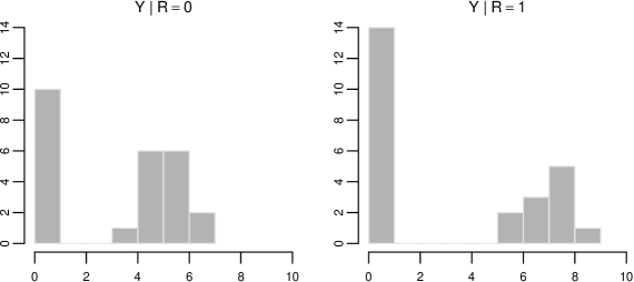
Figure 1: Histograms of the outcome for the example data stratified by treatment group.

The observed difference in means for the combined outcome, $\Delta$ in Equation (2), is 0.018 and both a two-sample t-test and a Wilcoxon rank sum test show highly insignificant effects of the treatment with p-values of 0.984 and 0.696 respectively. In order to analyse the data using proposed method we use the function truncComp as follows

model <- truncComp(Y ~ R, atom = 0, data = TruncCompExample, method="SPLRT")

where the formula interface is similar to other regression models implemented in R. The argument atom identifies the value assigned to the unobserved outcomes, and method can be SPLRT or LRT for either the semi-parametric or the parametric likelihood ratio test, respectively. In this example we have opted for the semi-parametric version to show how easily this additional flexibility is included. We obtain the results of the estimation by a calling the function summary on the estimated model:

summary(model)

## Estimation method: Semi-empirical Likelihood Ratio Test
## Confidence level = 95%
##
## Treatment contrasts
##                                          Estimate  CI Lower CI Upper
## Difference in means among the observed: 1.8564296 1.1638863 2.480132
## Odds ratio of being observed:           0.5238095 0.1660407 1.596820
##
## Joint test statistic: W = 31.09545
## p-value: p = 1.768924e-07

The output from the call to summary displays estimates for the two treatment contrasts corresponding to $\mu_{\delta}$ and $e^{\alpha_{\delta}}$ in Equations (4) and (5). These contrasts quantify the difference in means among the observed outcomes and the odds ratio of being observed respectively in accordance with the model specification. Each estimated treatment contrast is accompanied with a confidence interval, and finally the output displays the joint likelihood ratio test statistic and the associated $p$-value for the joint null-hypothesis of no treatment effect.

From the output we see that the semi-parametric likelihood ratio analysis reports an extremely low $p$-value for null-hypothesis of no joint treatment effect. This strongly contradicts the conclusions from both the previous $t$- and Wilcoxon analyses. The confidence intervals for the two treatment contrasts indicate that the average value for the observed outcome in the group defined by $R=1$ is significantly higher than the average value for the observed outcome in the group with $R=0$.

The confidence intervals can also be obtained by calling the function confint on the model object. This command reports both the marginal confidence intervals for the two treatment contrasts as well as a their simultaneous confidence region. To obtain the simultaneous confidence region we write

confint(model, type="simultaneous", plot=TRUE, resolution = 50)

where resolution is the number of grid points on which the surface is evaluated. Figure 2 shows a heat-map of the semi-empirical likelihood surface as well as the $95\%$ confidence region. The point $(0,0)$ is far outside of the joint confidence region which corresponds to the strong rejection of the joint null hypothesis of nu treatment effect.

Figure 2: Simultaneous empirical likelihood ratio surface for the two treatment contrasts.

4 Simulation study

To illustrate the power benefit and small sample properties of our proposed procedure we consider 4 setups, which we examine by simulations. In all simulations setups it is assumed that treatment is randomized 1:1. We will vary both the mean among survivors (denoted $\mu_{0}$ and $\mu_{1}$) and probability of death ($p_{0}$ and $p_{1}$). For the first three simulation setup values among survivors are assumed to follow a normal distribution with unit variance and the stated means. We will also consider the effect of heavily right skewed data among the survivors (simulation setup 4, which uses the square of a t-distribution with 2 degrees of freedom multiplicatively scaled to having the right mean. Table 1 below presents the considered simulation setups. It is noted that in simulation setups 3 and 4 the effect on the survivors and the effect on mortality are in opposite directions.

Table 1: Simulation setups. $\Delta$ denotes the marginal mean when setting the outcome to zero for the dead.

	$\mu_{0}$	$\mu_{1}$	$\pi_{0}$	$\pi_{1}$	Distribution	$\Delta$
Setup 1	3.0	4.0	0.35	0.35	Normal (sd=1)	-0.3476400
Setup 2	3.5	3.5	0.40	0.30	Normal (sd=1)	0.3481800
Setup 3	3.0	4.0	0.40	0.30	Normal (sd=1)	0.0035646
Setup 4	3.0	4.0	0.40	0.30	t-dist (df=2) squared	-1.0058211

To assess power we vary the sample size from 25 to 250 and for each configuration we conduct 100,000 Monte Carlo replications and compute power. The resulting power curves are presented in Figure 3. In setup 1 we observe a large power gain compared to the Wilcox test. Here the Wilcox tests gets “confused” by the large number of ties in the atom. In setup 2 Wilcox test has slightly better power profile. This is to be expected as our novel test is here disadvantaged by being a two-degrees-of-freedom test where the Wilcox is only one. It is further observed that Wilcox as expected as very little power when the effects on mortality and among survivors are of opposite sign despite the two distributions being markedly different indicating clear treatment effect (setups 3 and 4). In contrast our novel methods has excellent power. In all settings with a normally distributed outcome among survivors the parametric and semi-parametric approaches are similar, but for the heavy tail setup (no. 4) the semi-parametric approach is clearly superior.

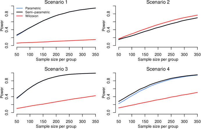
Figure 3: Simulated power as a function of sample size for each of the four scenarios in Table 1.

5 Discussion

In this paper we introduce a novel statistical test to assess treatment effect on continuous outcomes where one value has special meaning (e.g., all diseased are assigned lowest possible value). The procedure in potentially much more power-full than the current best-practice which is to use Wilcox-type tests. The proposed method includes both a fully parametric approach and a semi-parametric where one makes no assumptions on the functional form of the continuous part of the distribution. In all settings the new method not only provide an effect measure but also effect parameters with associated confidence intervals. The test is implemented in an R package available on GitHub.

It is noted that unlike the Wilcox test out proposed method can easily be extended to include covariates (A. Owen 1991). It is therefor not only useful in an RCT setting but also to observed data.

References

Jensen, Andreas Kryger, and Theis Lange. 2018. “The TruncComp R package for Two-Sample Comparison of Truncated Continuous Outcomes Using Parametric and Semi-Empirical Likelihood.” https://github.com/aejensen/TruncComp.

Owen, Art. 1991. “Empirical Likelihood for Linear Models.” The Annals of Statistics, 1725–47.

Owen, Art B. 1988. “Empirical Likelihood Ratio Confidence Intervals for a Single Functional.” Biometrika 75 (2): 237–49.

Wilks, Samuel S. 1938. “The Large-Sample Distribution of the Likelihood Ratio for Testing Composite Hypotheses.” The Annals of Mathematical Statistics 9 (1): 60–62.

Appendix

Derivation of semi-parametric test quantity

The empirical likelihood ratio function that compares the empirical maximum likelihood under a constraint set $\mathcal{C}$ to an unconstrained maximum likelihood is given by

$$R_{1,n}^{\text{E}}(\mathcal{C}) =\frac{\sup\limits_{\left\{p_{i}\right\}}\left(\prod_{i\in\mathcal{I}_{0}}p_{i}\mid\mathcal{C}\right)\sup\limits_{\left\{q_{j}\right\}}\left(\prod_{j\in\mathcal{I}_{1}}q_{j}\mid\mathcal{C}\right)}{\sup\limits_{F\in\mathcal{F}}\prod_{i\in\mathcal{I}_{0}}F(\left\{Y_{i}\right\})\sup\limits_{G\in\mathcal{F}}\prod_{j\in\mathcal{I}_{1}}G(\left\{Y_{j}\right\})}$$ (11)

where $\mathcal{F}$ is the family of cadlag functions. This empirical likelihood ratio is simply a comparison between the non-parametric unconstrained maximum likelihood values and a a null-model where the maximum likelihoods in the two treatment groups are constrained according to a constraint set $\mathcal{C}$. The sets of weights, $\left\{p_{i}\right\}$ and $\left\{q_{j}\right\}$, form a constrained multinomial distribution over the observations.

It is well-known that the solutions to the two unconstrained maximizations in the denominator are given by the empirical distribution functions that put equal weight on each observation. From here it follows that the likelihood ratio function can be written as

$$R_{1,n}^{\text{E}}(\mathcal{C}) =\sup\limits_{\left\{p_{i}\right\},\left\{q_{j}\right\}}\left(\prod_{i\in\mathcal{I}_{0}}|\mathcal{I}_{0}|p_{i}\prod_{j\in\mathcal{I}_{1}}|\mathcal{I}_{1}|q_{j}\mid\mathcal{C}\right)$$ (12)

where $|\cdot|$ denotes the cardinality of the index set.

The constraint set is chosen so that $\left\{p_{i}\right\}$ and $\left\{q_{j}\right\}$ are bona fide multinomial distributions, and so that the expected value of the observations with indices in $\mathcal{I}_{0}$ have expectation $\beta$ and the difference between the expectations comparing the observations with indices in $\mathcal{I}_{1}$ to those with indices in $\mathcal{I}_{0}$ is given by $\beta_{\delta}$ similar to the structure of the linear model in Equation (5). This yields the following set of constraints:

$$p_{i} \geq 0, \quad\sum_{i\in\mathcal{I}_{0}}p_{i} =1, \sum_{i\in\mathcal{I}_{0}}p_{i}(Y_{i}-\beta)=0$$ (13)

$$q_{j} \geq 0, \quad\sum_{j\in\mathcal{I}_{1}}q_{j} =1, \sum_{j\in\mathcal{I}_{1}}q_{j}(Y_{j}-\beta-\beta_{\delta})=0$$ (14)

The find the values of $\left\{p_{i}\right\}$ and $\left\{q_{j}\right\}$ in Equation (12) that satisfies the constraint set we solve the constrained optimization problem through the following objective function

$$O(\left\{p_{i}\right\},\left\{q_{j}\right\}) =\sum_{i\in\mathcal{I}_{0}}\log(|\mathcal{I}_{0}|p_{i})+\sum_{j\in\mathcal{I}_{1}}\log(|\mathcal{I}_{1}|q_{j})+\gamma_{1}\left(\sum_{i\in\mathcal{I}_{0}}p_{i}-1\right)+\gamma_{2}\left(\sum_{j\in\mathcal{I}_{1}}q_{j}-1\right)$$ (15)

$$-|\mathcal{I}_{0}|\lambda_{1}\sum_{i\in\mathcal{I}_{0}}p_{i}(Y_{i}-\beta)-|\mathcal{I}_{1}|\lambda_{2}\sum_{j\in\mathcal{I}_{1}}q_{j}(Y_{j}-\beta-\beta_{\delta})$$

where $\gamma_{1}$, $\gamma_{2}$, $\lambda_{1}$ and $\lambda_{2}$ are Lagrange multipliers.

Calculating the partial derivatives of $O(\left\{p_{i}\right\},\left\{q_{j}\right\})$ with respect to $p_{i}$ and $q_{i}$ and setting them equal to zero we have that

$$0 =\frac{\partial}{\partial p_{i}}O(\left\{p_{i}\right\},\left\{q_{j}\right\})=\frac{1}{p_{i}}-|\mathcal{I}_{0}|\lambda_{1}(Y_{i}-\beta)+\gamma_{1}$$ (16)

$$0 =\frac{\partial}{\partial q_{j}}O(\left\{p_{i}\right\},\left\{q_{j}\right\})=\frac{1}{q_{j}}-|\mathcal{I}_{1}|\lambda_{2}(Y_{j}-\beta-\beta_{\delta})+\gamma_{2}$$ (17)

and by applying the constrains it follows that

$$0 =\sum_{i\in\mathcal{I}_{0}}p_{i}\frac{\partial O(\left\{p_{i}\right\},\left\{q_{j}\right\})}{\partial p_{i}}$$ (18)

$$=\sum_{i\in\mathcal{I}_{0}}p_{i}\left(\frac{1}{p_{i}}-|\mathcal{I}_{0}|\lambda_{1}(Y_{i}-\mu)+\gamma_{1}\right)$$

$$=\sum_{i\in\mathcal{I}_{0}}1-|\mathcal{I}_{0}|\lambda_{1}\sum_{i\in\mathcal{I}_{0}}p_{i}(Y_{i}-\beta)+\gamma_{1}\sum_{i\in\mathcal{I}_{0}}p_{i}$$

$$=|\mathcal{I}_{0}|+\gamma_{1}$$

Therefore $\gamma_{1}=-|\mathcal{I}_{0}|$ and $\gamma_{2}=-|\mathcal{I}_{1}|$ by similar calculation for $q_{j}$. From Equations (16) and (17) and the previous results we obtain the following solutions

$$p_{i}=\frac{1}{|\mathcal{I}_{0}|(1+\lambda_{1}(Y_{i}-\beta))},\quad q_{j}=\frac{1}{|\mathcal{I}_{1}|(1+\lambda_{2}(Y_{j}-\beta-\beta_{\delta}))}$$ (19)

and by inserting these expressions into the expression for the empirical likelihood ratio we obtain

$$\log R_{1,n}^{E}(\beta,\beta_{\delta}) =\sum_{i\in\mathcal{I}_{0}}\log(|\mathcal{I}_{0}|p_{i})+\sum_{j\in\mathcal{I}_{1}}\log(|\mathcal{I}_{1}|q_{j})$$ (20)

$$=\sum_{i\in\mathcal{I}_{0}}\log\frac{1}{1+\lambda_{1}(Y_{i}-\beta)}+\sum_{j\in\mathcal{I}_{1}}\log\frac{1}{1+\lambda_{2}(Y_{j}-\beta-\beta_{\delta})}$$

$$=-\sum_{i\in\mathcal{I}_{0}}\log\left(1+\lambda_{1}(Y_{i}-\mu)\right)-\sum_{j\in\mathcal{I}_{1}}\log\left(1+\lambda_{2}(Y_{j}-\beta-\beta_{\delta})\right)$$

The values of $\lambda_{1}$ and $\lambda_{2}$ can then be found by combining Equations (16) and (17) with the constraints leading to the following set of equations

$$|\mathcal{I}_{0}|^{-1}\sum_{i\in\mathcal{I}_{0}}\frac{Y_{i}-\beta}{1+\lambda_{1}(Y_{i}-\beta)}=0,\quad|\mathcal{I}_{1}|^{-1}\sum_{j\in\mathcal{I}_{1}}\frac{Y_{j}-\beta-\beta_{\delta}}{1+\lambda_{2}(Y_{j}-\beta-\beta_{\delta})}=0$$ (21)

that in practice can be solved for $\lambda_{1}$ and $\lambda_{2}$ using a numerical root finding method.

The empirical LRT statistic is therefore

$$W_{1,n}^{E}(\beta,\beta_{\delta}) =-2\log R_{1,n}^{E}(\beta,\beta_{\delta})$$ (22)

$$=2\left(\sum_{i\in\mathcal{I}_{0}}\log\left(1+\lambda_{1}(Y_{i}-\beta)\right)+\sum_{j\in\mathcal{I}_{1}}\log\left(1+\lambda_{2}(Y_{j}-\beta-\beta_{\delta})\right)\right)$$

where $W_{1,n}^{E}(\beta_{\delta}^{\ast})=\sup\limits_{\beta}W_{1,n}^{E}(\beta,\beta_{\delta}^{\ast})$ the profile version testing the difference between treatments.