Covariant Bethe - Salpeter approximation in strongly correlated electron systems model

Abstract

Strongly correlated electron systems are generally described by tight binding lattice Hamiltonians with strong local (on site) interactions, the most popular being the Hubbard model. Although the half filled Hubbard model can be simulated by Monte Carlo(MC), physically more interesting cases beyond half filling are plagued by the sign problem. One therefore should resort to other methods. It was demonstrated recently that a systematic truncation of the set of Dyson - Schwinger equations for correlators of the Hubbard, supplemented by a “covariant” calculation of correlators leads to a convergent series of approximants. The covariance preserves all the Ward identities among correlators describing various condensed matter probes. While first order (classical), second (Hartree - Fock or gaussian) and third (Cubic) covariant approximation were worked out, the fourth (quartic) seems too complicated to be effectively calculable in fermionic systems. It turns out that the complexity of the quartic calculation in local interaction models,is manageable computationally. The quartic (Bethe - Salpeter type) approximation is especially important in 1D and 2D models in which the symmetry broken state does not exists (the Mermin - Wagner theorem), although strong fluctuations dominate the physics at strong coupling. Unlike the lower order approximations, it respects the Mermin - Wagner theorem. The scheme is tested and exemplified on the single band 1D and 2D Hubbard model.

I Introduction

Strongly correlated electron systems like the high critical temperature cuprate superconductorsDagotto (1994); Scalapino (2012), quantum magnetsFradkin (2013), etc. are currently a topic of great interest in condensed matter physics. These materials, both three dimensional (3D), layered or recently fabricated 2D materialsGibertini et al. (2019) typically (but not always) involve hybridization of the $d$ or $f$  atomic orbitals. Unfortunately understanding of physics of this class of materials hinges on at least qualitative understanding of the simplest models like the one band Hubbard model on square lattice. Although the Hamiltonian of the model, often just a nearest neighbor tunneling and strong (large $U$) local (on site) interactions, is deceptively simple, exact solutionLieb and Wu (1968) exists only in 1D. Moreover even in 1D it is limited to specific quantities like the distribution of momenta. Green’s functions that are directly measured in ARPES experiments or susceptibilities measured in magnetization or optical experiments have not been calculated exactly. Alternatively one can solve yet smaller Hubbard -like systems on periodic “crystallites” around $16$ sites by exact diagonalizationWeiße and Fehske (2007). Therefore one has to resort to approximations of various kinds.

A straightforward approach is the path integral Monte CarloBecca and Sorella (2017) simulation of fermionic systems. Unfortunately the sign problem immediately arises in the case of interests. The simple half filled Hubbard model has no sign problem due to the electron hole symmetry; however, for example the high temperature superconductivity occurs at nonzero doping, when the electron - hole symmetric condition is violated. In most cases of interest the sign problem therefore does not allow simulation. An alternative is a diagrammatic approximation scheme or some other analytic methods. Most start with an (infinite) hierarchy of relations between correlators known as Dyson - Schwinger equations (DSE). This infinite system of generally nonlinear equations should be somehow disentangled. This can be done either by devising some kind of perturbation theory (weak, strong coupling, large “$N$” expansion etc) or directly by truncating the equations according to some “principle”, like variational or otherAlbrecht et al. (1998); Onida et al. (2002).

The quality of a truncation is usually dependent on preserving general relations like conservation laws and “sum rules”Baym and Kadanoff (1961); Haussmann et al. (2007). This is highly nontrivial and several strategies were attemptedLeBlanc et al. (2015). A general method to preserve the Ward - Takahashi identity(WTI) in an approximation scheme was developed long time agoKovner and Rosenstein (1989) in the context of field theory as the covariant gaussian approximation (CGA) to solve unrelated problems in quantum field theory and superfluidityRosenstein and Kovner (1989a, b); Li et al. (2012); Zhang and Li (2013). A non-perturbative variational gaussian method that originated in quantum mechanics of atoms and molecules in relativistic theories like the standard model of particle physics has several serious related problems. First, the wave function renormalization requires a dynamical description. Second, the Green’s functions obtained using the naive gaussian approximation violates the charge conservation. In particular the most evident problem is that the Goldstone bosons resulted from spontaneous breaking of continuous symmetry are massive. The method is thus considered dubious or inconsistent. Both problems were solved by an observation that the solutions of the minimization equations are not necessarily equivalent to the variational Green’s functions. This results in the covariant gaussian approximation (CGA).

It was demonstrated recentlyRosenstein and Li (2018) (using a simple example) that a systematic truncation of the set of Dyson - Schwinger equations for correlators of the Hubbard, supplemented by a “covariant” calculation of correlators, leads to a converging series of approximants. The covariance preserves all the Ward identities among correlators describing various condensed matter probes. While first order (classical) second order (Hartree - Fock or gaussian) and third order (cubic) approximations have been worked out, the fourth order seems too complicated to be effectively calculable in fermionic systems without symmetry breaking. This is especially important in 1D and 2D models in which the symmetry broken state does not exist (due to the Mermin - Wagner theoremMermin and Wagner (1966); Mermin (1967)), although strong anti - ferromagnetic (AF) fluctuations dominate the physics at strong coupling. Unlike lower order approximations, the quartic covariant scheme already respects the Mermin - Wagner theorem.

It is shown in the present paper that the complexity of covariant quartic approximation (CQA) in Hubbard model can be reduced to a manageable level due to locality of interactions. There is a possibility of transitions between the coordinate and the momentum spaces that reduces the computation cost. We focus on the electron correlator describing the electron (hole) excitations measured in photoemission and other condensed matter probes. The scheme is tested and exemplified on solvable 1D finite site Hubbard model (including beyond half filling) and on a more physically important 2D Hubbard model at half filling in which reliable Monte Carlo simulations exist.

The paper is organized as follows. In section II the sequence of covariant approximations is developed using the simplest possible quantum model: the one dimensional quantum anharmonic oscillator. Next in section III the CQA is developed for a general fermionic system and is applied to the one band Hubbard model in Section IV. In Section V, the implementation is described and the results are compared with exact solutions(1D) and Monte Carlo results(2D). An estimate of complexity of application of CQA to a realistic 2D material are subject of Section VI. Discussion and conclusions are presented in Section VII.

II Hierarchy of covariant truncations of Dyson - Schwinger equations in a bosonic model

The main idea and methodology behind the covariant approximants are presented in this section in the simplest possible setting: thermodynamics of the bosonic field (often used as an “order parameter”Amit and Martin-Mayor (2005); Chaikin et al. (1995)). Later the most advanced fourth in a series of such approximant for a many - body fermionic system will be developed and shown to be computationally practical.

II.1 An exactly solvable “bosonic” model: 1D classical statistical system (quantum mechanics of the 1D anharmonic oscillator)

The simplest nontrivial model having many of the basic ingredients of the interacting electronic system is the one dimensional scalar field theory viewed as the thermodynamic 1D Ginzburg - Landau -Wilson modelAmit and Martin-Mayor (2005); Chaikin et al. (1995) (equivalently via Feynman path integralNegele and Orland (1988) to the quantum mechanics of the anharmonic oscillator). The quantity describing the thermal fluctuations of the field is the Boltzmann factor:

$$F\left[J\right]\equiv H\left[J\right]/T=\int_{x=-\infty}^{\infty}\left\{-\frac{1}{2}\psi_{x}\partial^{2}\psi_{x}+\frac{a}{2}\psi_{x}^{2}+\frac{1}{4}\psi_{x}^{4}-J_{x}\psi_{x}\right\}.$$ (1)

The scale and the field normalization are chosen in a way to make the coefficient of the gradient term to be $1/2$ and that of the interaction term $1/4$. Here $J_{x}$ is an external “source”, a convenient theoretical device to generate connected correlatorsAmit and Martin-Mayor (2005); Chaikin et al. (1995)

$$W\left[J\right] = -\ln\int_{\psi}e^{-F\left[J\right]}$$ (2)

$$G_{x_{1}...x_{n}} = -\frac{\delta}{\delta J_{x_{1}}}...\frac{\delta}{\delta J_{x_{n}}}W\left[J\right]\equiv\left\langle\psi_{x_{1}}...\psi_{x_{n}}\right\rangle$$

II.2 The main idea of the approximation

The CQA is derived following the line of reasoning used to obtain other covariant approximations, gaussian and cubic in Refs. Wang et al., 2017; Rosenstein and Li, 2018. It is based on the set of Dyson-Schwinger equations(DSE). Here however we go one step further by considering the truncation of DSE up to the four field correlator. The hierarchy of DSE for the connected correlators contains, the first equation for a nonvanishing source,

$$J_{x}=\left(-\partial^{2}+a\right)\varphi_{x}+\varphi_{x}^{3}+3\varphi_{x}G_{xx}+G_{xxx};$$ (3)

also called the “equation of motion”. Here the field expectation value in the presence of the source is denoted by $\varphi_{x}\equiv\left\langle\psi_{x}\right\rangle$. The second equation, obtained by the functional differentiation with respect to the source, is:

$$\delta\left(x_{1}-x_{2}\right) =\left(-\partial_{x_{1}}^{2}+a+3\varphi_{x_{1}}^{2}\right)G_{x_{2}x_{1}}+3G_{x_{2}x_{1}}G_{x_{1}x_{1}}$$ (4)

$$+3\varphi_{x_{1}}G_{x_{2}x_{1}x_{1}}+G_{x_{2}x_{1}x_{1}x_{1}}\text{.}$$

The third equation,

$$0 =\left(-\partial_{x_{1}}^{2}+a+3\varphi_{x_{1}}^{2}+3G_{x_{1}x_{1}}\right)G_{x_{3}x_{2}x_{1}}+6\varphi_{x_{1}}G_{x_{3}x_{1}}G_{x_{2}x_{1}}$$ (5)

$$+3G_{x_{2}x_{1}}G_{x_{3}x_{1},x_{1}}+3G_{x_{3}x_{1}}G_{x_{2}x_{1}x_{1}}+3\varphi_{x_{1}}G_{x_{3}x_{2}x_{1},x_{1}}+G_{x_{3},x_{2},x_{1},x_{1},x_{1}},$$

if written in full. The last term is the five point correlator and thus will be omitted within the fourth order approximation,

$$0 =\left(-\partial_{x_{1}}^{2}+a+3\varphi_{x_{1}}^{2}+3G_{x_{1}x_{1}}\right)G_{x_{3}x_{2}x_{1}}+6\varphi_{x_{1}}G_{x_{3}x_{1}}G_{x_{2}x_{1}}$$ (6)

$$+3G_{x_{2}x_{1}}G_{x_{3}x_{1}x_{1}}+3G_{x_{3}x_{1}}G_{x_{2}x_{1}x_{1}}+3\varphi_{x_{1}}G_{x_{3}x_{2}x_{1}x_{1}},$$

The fourth DSE is already too cumbersome to write in full. Here only even correlators are retained (with correlators up to the four field):

$$0 = \left(-\partial_{x_{1}}^{2}+a+3G_{x_{1}x_{1}}\right)G_{x_{4}x_{3}x_{2}x_{1}}+6G_{x_{4}x_{1}}G_{x_{3}x_{1}}G_{x_{2}x_{1}}+3G_{x_{2}x_{1}}G_{x_{4}x_{3}x_{1}x_{1}}$$

$$+3G_{x_{3}x_{1}}G_{x_{4}x_{2}x_{1}x_{1}}+3G_{x_{4}x_{1}}G_{x_{3}x_{2}x_{1}x_{1}}+...\text{.}$$

The “…” refers to terms containing odd correlators, namely $\varphi_{x}$ or three field correlators. In the next subsection it will be argued that symmetry makes odd correlators redundant.

The set of equations continues to higher orders and will become too complicated. However at least far from second order phase transition point (criticality) it is natural to assume a clustering hypothesis: higher connected correlators are “smaller” in most models describing (even strongly coupled) physical systems. The covariant truncation is one of the proposals to truncate the infinite set of increasingly complicated equations using the symmetry and consistency arguments.

II.3 The truncation of the DSE set and the symmetry considerations

The “quartic covariant” truncation of the infinite set of equations is achieved by taking $G_{x_{1}...x_{i}}=0,$ for all $i>4$. The set for $J_{x}=0$

$$0=\left(-\partial^{2}+a\right)\varphi_{x}+\varphi_{x}^{3}+3\varphi_{x}G_{xx}^{tr}+G_{xxx}^{tr};$$ (8)

$$\delta\left(x_{1}-x_{2}\right)=\left(-\partial_{x_{1}}^{2}+a+3\varphi_{x_{1}}^{2}\right)G_{x_{2}x_{1}}^{tr}+3G_{x_{2}x_{1}}^{tr}G_{x_{1}x_{1}}^{tr}+3\varphi_{x_{1}}G_{x_{2}x_{1}x_{1}}^{tr}+G_{x_{2}x_{1}x_{1}x_{1}}^{tr};$$

$$0=\left(-\partial_{x_{1}}^{2}+a+3\varphi_{x_{1}}^{2}\right)G_{x_{3}x_{2}x_{1}}^{tr}+6\varphi_{x_{1}}G_{x_{3}x_{1}}^{tr}G_{x_{2}x_{1}}^{tr}+3G_{x_{1}x_{1}}^{tr}G_{x_{3}x_{2}x_{1}}^{tr}+3G_{x_{2}x_{1}}^{tr}G_{x_{3}x_{1}x_{1}}^{tr}+3G_{x_{3}x_{1}}^{tr}G_{x_{2}x_{1}x_{1}}^{tr}+3\varphi_{x_{1}}G_{x_{3}x_{2}x_{1}x_{1}}^{tr};$$

$$0=\left(-\partial_{x_{1}}^{2}+a\right)G_{x_{4}x_{3}x_{2}x_{1}}^{tr}+6G_{x_{4}x_{1}}^{tr}G_{x_{3}x_{1}}^{tr}G_{x_{2}x_{1}}^{tr}+3G_{x_{1}x_{1}}^{tr}G_{x_{4}x_{3}x_{2}x_{1}}^{tr}+3G_{x_{2}x_{1}}^{tr}G_{x_{4}x_{3}x_{1}x_{1}}^{tr}+3G_{x_{3}x_{1}}^{tr}G_{x_{4}x_{2}x_{1}x_{1}}^{tr}+3G_{x_{4}x_{1}}^{tr}G_{x_{3}x_{2}x_{1}x_{1}}^{tr}+...\text{,}$$

will be called the “minimization equations”. They will determine the “truncated” correlators that should be distinguishedKovner and Rosenstein (1989); Wang et al. (2017) from  an approximant to the “physical” correlators defined in Eq.(2).

Moreover in many cases symmetry simplifies the set of equations. In our case the Hamiltonian, Eq.(1) has the global $Z_{2}$ symmetry $\psi_{x}\rightarrow-\psi_{x}$ that will be preserved in the covariant approach. The symmetry allows to conclude that $\varphi_{x}^{tr}=G_{x_{1},x_{2},x_{3}}^{tr}=0$. Then the first and third equations are automatically satisfied, and the remaining second and fourth will be simplified to

$$\delta\left(x_{1}-x_{2}\right)=\left(-\partial_{x_{1}}^{2}+a\right)G_{x_{2}x_{1}}^{tr}+3G_{x_{2}x_{1}}^{tr}G_{x_{1}x_{1}}^{tr}+G_{x_{2}x_{1}x_{1}x_{1}}^{tr};$$ (9)

$$\left(-\partial_{x_{1}}^{2}+a\right)G_{x_{4}x_{3}x_{2}x_{1}}^{tr}+6G_{x_{4}x_{1}}^{tr}G_{x_{3}x_{1}}^{tr}G_{x_{2}x_{1}}^{tr}+3G_{x_{1}x_{1}}^{tr}G_{x_{4}x_{3}x_{2}x_{1}}^{tr}$$ (10)

$$+3G_{x_{2}x_{1}}^{tr}G_{x_{4}x_{3}x_{1}x_{1}}^{tr}+3G_{x_{3}x_{1}}^{tr}G_{x_{4}x_{2}x_{1}x_{1}}^{tr}+3G_{x_{4}x_{1}}^{tr}G_{x_{3}x_{2}x_{1}x_{1}}^{tr}=0\text{.}$$

The first equation is commonly called “gap equation” due to similarity with the corresponding equation in the superconductivity theory, while the second is similar, but not equivalent to the “Bethe - Salpeter” equation for the bound states. We address this issue later after using the translation invariance of the equations.

II.4 Covariant vs “naive” correlator

The connected correlators are obtained by differentiations of the field shift $\varphi_{x}$ with respect to the sources, and subsequently taken at $J=0$,

$$G_{x_{1}...x_{n}}\equiv\frac{\delta}{\delta J_{x_{1}}}...\frac{\delta}{\delta J_{x_{n-1}}}\varphi_{x_{n}}|_{J_{x_{i}}=0}\text{,}$$ (11)

where $\varphi_{x_{n}}$ is given by the solution via Eqs.(3,4,6,II.2). The correlators obtained in that way are not necessarily equal to truncated functions that appear in the minimization equations Eq.(8). Sometimes $G^{tr}$ in the minimization equations are treated as approximate correlators both for $I=2$ (gaussian) and $I=4$ (Bethe - Salpeter). We will refer to these as “naive” noncovariant approach. In these cases one often discovers that a symmetry, like the $Z_{2}$ are not respected. Generally it is found that so called Ward identities (relations between various Green’s functions derived from the symmetry) are not obeyed by the approximate correlators. In extreme cases, for example when a continuous symmetry is spontaneously  broken, Ward identities like the Goldstone theorem are violated. As will be discussed below, even the antisymmetry of the fermionic correlators (the Fermi symmetry) is violated in the naive truncation approaches. One expects that the covariant approximation results are more accurate.

The method was compared with available exact results for the S-matrix in the Gross - Neveu modelRosenstein and Kovner (1989c) (a local four Fermion interactions in 1D Dirac excitations recently considered in condensed matter physics) and with MC simulations in various scalar models, see Ref.Wang et al., 2017 . Applied to the electronic field correlator in electronic systems, CGA becomes roughly equivalent to Hartree - Fock (HF) approximation that is generally not precise enough. Its covariance might improve the calculation of the four fermion correlators like the density - density, but to address quantitatively photoemission or other direct electron or hole excitation probes, a more precise method is needed.

The covariant correlators $G_{x_{1}...x_{n}}$ could be different from $G_{x_{1}...x_{n}}^{tr}$, and the covariant correlators satisfy the Ward identities Wang et al. (2017); Rosenstein and Li (2018). In our case, differentiating Eq.(3), one obtains:

$$\delta\left(x_{1}-x_{2}\right)=\left(-\partial_{x_{1}}^{2}+a+3\varphi_{x_{1}}^{2}+3G_{x_{1}x_{1}}^{tr}\right)G_{x_{2}x_{1}}+3\varphi_{x_{1}}\frac{\delta G_{x_{1}x_{1}}^{tr}}{\delta J_{x_{2}}}+\frac{\delta G_{x_{1}x_{1}x_{1}}^{tr}}{\delta J_{x_{2}}}\text{.}$$ (12)

Of course in 1D symmetry is not spontaneously broken and thus $\varphi_{x}$ vanishes, so that the covariant correlator obeys

$$\delta\left(x_{1}-x_{2}\right)=\left(-\partial_{x_{1}}^{2}+a+3G_{x_{1}x_{1}}^{tr}\right)G_{x_{2}x_{1}}+\frac{\delta G_{x_{1}x_{1}x_{1}}^{tr}}{\delta J_{x_{2}}}$$ (13)

The derivative $\frac{\delta G_{x_{1}x_{2}x_{3}}^{tr}}{\delta J_{x_{4}}}$, often called the “chain correction” (due to its diagrammatic interpretationKovner and Rosenstein (1989)), is obtained by differentiating the third DS equation, Eq.(6) with respect to $J$ (and omitting the odd correlators, as above):

$$\left(-\partial_{x_{1}}^{2}+a+3G_{x_{1}x_{1}}^{tr}\right)\frac{\delta G_{x_{3}x_{2}x_{1}}^{tr}}{\delta J_{x_{4}}}+3G_{x_{2}x_{1}}^{tr}\frac{\delta G_{x_{3}x_{1}x_{1}}^{tr}}{\delta J_{x_{4}}}+3G_{x_{3}x_{1}}^{tr}\frac{\delta G_{x_{2}x_{1}x_{1}}^{tr}}{\delta J_{x_{4}}}$$

$$= -6G_{x_{4}x_{1}}G_{x_{3}x_{1}}^{tr}G_{x_{2}x_{1}}^{tr}-3G_{x_{4}x_{1}}G_{x_{3}x_{2}x_{1}x_{1}}^{tr}\text{.}$$

Note that the chain equation is generally linear in chain variable. This is crucial for an ability to calculate the approximation. It will be demonstrated in the next section that in the particular case of the local scalar model (in unbroken symmetry phases only), the truncated and the full two field correlators (or so called the green functions) in fact coincide. This general observation simplifies the calculation of the correlator since one just needs to solve the minimization equations.

II.5 Translation invariance and solution of minimization equations

We consider in the present paper only translation symmetric phases. The translation symmetry greatly simplifies the solution of the nonlinear minimization equations by making the Fourier transformation of the Green functions. In our case only two are required:

$$G_{x_{1}x_{2}}^{tr} = \frac{1}{2\pi}\int_{k}g_{k}^{tr}e^{-ik\left(x_{1}-x_{2}\right)},$$ (15)

$$G_{x_{4}x_{3}x_{2}x_{1}}^{tr} = \frac{1}{\left(2\pi\right)^{3}}\int_{k_{1}k_{2}k_{3}}g_{k_{1}k_{2}k_{3}}^{tr}e^{-ik_{1}\left(x_{1}-x_{2}\right)}e^{-ik_{2}\left(x_{2}-x_{4}\right)}e^{-ik_{3}\left(x_{3}-x_{4}\right)}\text{.}$$

We denote $g_{k}^{tr}$ as $g_{k}$ because the covariant green function is equal to the two field correlator solution of the minimization equations. The equations Eq.(9) and Eq.(10) then take a form:

$$\left(k^{2}+a+3b\right)g_{k}+\frac{1}{2\pi}\text{$\int$}_{k_{1}}q_{kk_{1}} = 1;$$ (16)

$$\left(\left(k_{1}+k_{2}+k_{3}\right)^{2}+a+3b\right)g_{k_{1}k_{2}k_{3}}^{tr}+3g_{k_{3}}q_{k_{1}k_{2}}+3g_{k_{2}}q_{k_{1}k_{3}}+3g_{k_{1}}q_{k_{2}k_{3}} = -6g_{k_{1}}g_{k_{2}}g_{k_{3}}\text{,}$$

where the “bubble” $b$ and the “vertex” $q$ are defined as

$$b\equiv G_{xx}=\frac{1}{2\pi}\int_{k}g_{k};\text{ \ \ }$$ (17)

$$q_{k_{1}k_{2}}\equiv\frac{1}{2\pi}\int_{k}g_{k_{1}k_{2}k}^{tr}\text{.}$$ (18)

This nonlinear set of equations can be simplified as follows. Dividing the second Eq.(16) by $\left(\left(k_{1}+k_{2}+k_{3}\right)^{2}+a+3b\right)$, and integrating over $k_{3}$, one obtains a linear equation in $q$:

$$q_{k_{1}k_{2}}=-\frac{3}{2\pi}\int_{k}\left\{\frac{g_{k}q_{k_{1}k_{2}}+g_{k_{2}}q_{k_{1}k}+g_{k_{1}}q_{k_{2}k}}{\left(k_{1}+k_{2}+k\right)^{2}+a+3b}+\frac{2g_{k_{1}}g_{k_{2}}g_{k}}{\left(k_{1}+k_{2}+k\right)^{2}+a+3b}\right\}\text{.}$$ (19)

The first equation of Eq.(16) in the form,

$$g_{k_{1}}=\left(k^{2}+a+3b\right)^{-1}\left(1-\frac{1}{2\pi}\int_{k}q_{k_{1}k}\right)\text{,}$$ (20)

Eq.(17),Eq.(20) and Eq.(19) are finally solved by iterations. The results are presented next.

II.6 Comparison with exact results.

II.6.1 Numerical solution of the minimization equation

In order to solve the minimization equations, we chose a cut-off $k_{\Lambda}$,and assume that $g\left(k\right)=1/k^{2}$ for $\left|k\right|>k_{\Lambda}$ and $q\left(k_{1},k_{2}\right)=0$ for $\left|k_{1}\right|>k_{\Lambda}$ or $\left|k_{2}\right|>k_{\Lambda}$, and the assumption is justified by the asymptotical forms of $g\left(k\right)$ and $q\left(k_{1},k_{2}\right)$. Thus

$$b=\frac{1}{2\pi}\int_{-\infty}^{\infty}g\left(k\right)dk=\frac{1}{2\pi}\int_{-k_{\Lambda}}^{k_{\Lambda}}g\left(k\right)dk+\frac{1}{\pi k_{\Lambda}},$$ (21)

and other integrals can be approximated by replacing the integral bounds $\int_{-\infty}^{\infty}$ by the integration inside the cut-off $k_{\Lambda}$, $\int_{-k_{\Lambda}}^{k_{\Lambda}}$ plus $\int_{k_{\Lambda}}^{\infty}+\int_{-\infty}^{-k_{\Lambda}}$ using the asymptotical forms of $g\left(k\right)$ and $q\left(k_{1},k_{2}\right)$ .We enlarge $k_{\Lambda}$, until the final result converges. As for the finite integral $\int_{-k_{\Lambda}}^{k_{\Lambda}}$, we first split the integration interval into $N$ intervals and evaluate the value of each intervals using Bode’s rulePress et al. (2007), then we split the interval into $2N$ intervals and do it again until it converges. For the parameters we calculate, they all converge at cut-off $k_{\Lambda}=102.4$ and intervals $N=1024$.

II.6.2 Comparison with the exact result

The exact result can be obtained by analogue with the quantum anharmonic oscillator Wang et al. (2017); Rosenstein and Li (2018). We calculate $g_{k}$ for $a=$ $-1,0.5,0,1$ in Fig. 1 (the exact is in the red line ) and compare them with the results obtained by using GW, covariant gaussian approximation (CGA), covariant cubic approximation (CCA) and covariant quartic approximation (CQA). For example the worst precision of CQA at $a=0$ is around $1\%$ for the whole range of $k$ - vectors. For negative $a$, for example $a=-1$, the deviation is around $12\%$ at $k=0$ for CQA.

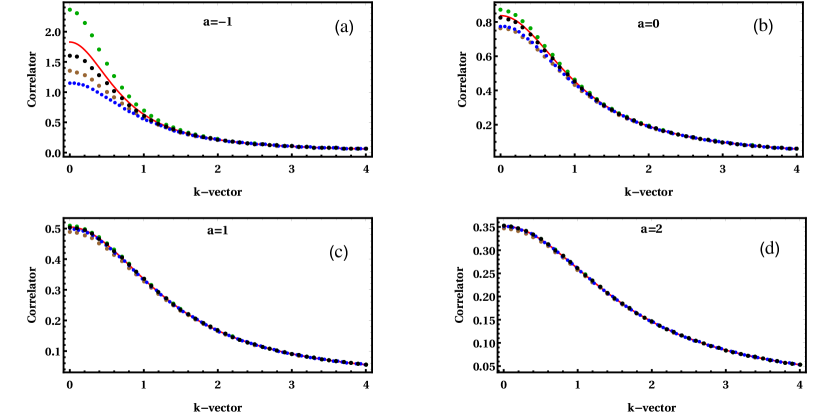
Figure 1: Comparison of GW, covariant gaussian approximation (CGA), covariant cubic approximation (CCA),covariant quartic approximation (CQA), and exact results for a 1D Ginzburg - Landau - Wilson chain (quantum mechanical anharmonic oscillator) $a=$ $-1,0.5,0,1$ respectively shown in (a),(b),(c),(d). The red line is the exact correlator, while blue, brown, the darker green, and black dots, are GW, CGA, CCA and CQA respectively.

III Quartic approximation in strongly interacting electronic systems

Generalization to many - body electron system within the field theoretical path integral framework is rather straightforward: the field becomes a Grassmannian function of (Matsubara) time, space and some other “flavours” like spin and valley indices. Still the Pauli principle makes the calculation simpler as is emphasized below in full generality. For example there is no expectation values of products of odd number of fermionic fields.

III.1 Four fermion interactions in the Nambu representation and DS equations.

Let us start with a general model of fermions described within the path integral approachNegele and Orland (1988) by a large number of complex Grassmannian variables $\psi^{a}$ and $\psi^{\ast a}$. All the usual indices like position in space, time, spin, band (valley), etc are lumped together in one “index” $a$. It is convenient to consider the two conjugate Grassmannians as real Grassmann numbers with an additional index $c$ taking two values $c=.$ (no star) and$\ c=\ast$. Then all the indices contained in $a$ and the charge (Nambu) index appear in the combined index $A=\left\{c,a\right\}$ on the same footing. The interaction is assumed to be of the two - body (four Fermi) variety common to the many - body electronic systems. The Matsubara action including the Grassmannian source generally has a form:

$$A\left[\psi,J\right]=\frac{1}{2}\psi^{A}T^{AB}\psi^{B}+\frac{1}{4!}V^{ABCD}\psi^{A}\psi^{B}\psi^{C}\psi^{D}-J^{A}\psi^{B}\text{.}$$ (22)

The antisymmetric matrix $T$ will be referred to as the “hopping” term. The coefficient the of interaction term, $V^{ABCD}$, is also antisymmetric in all four indices due to the Pauli symmetry.

General connected correlators are defined (similar to scalar fields, but note that the order of derivatives matters due to the Grassmannian algebra) by,

$$G^{A_{1}A_{2}...A_{n}}=-\frac{\delta^{n}F}{\delta J^{A_{1}}...\delta J^{A_{n}}}=\left\langle\psi^{A_{1}}...\psi^{A_{n}}\right\rangle\text{,}$$ (23)

where $F=-\log Z$ is the free energy with $Z=\int e^{-A\left[\psi,J\right]}$.

As with the scalar fields we start from derivation of the relevant DS equations via differentiation with respect to the source $J$. Then the covariant correlator is shown to be equal to the “truncated” one within a specific form of the minimization equations. The first in the series is the “off shell” (namely keeping the “source” $J$ nonzero) equation of state:

$$J^{A}=-T^{AX}\psi^{X}-\frac{1}{3!}V^{AX_{2}X_{3}X_{4}}\left(\psi^{X_{2}}\psi^{X_{3}}\psi^{X_{4}}+3\psi^{X_{2}}\left\langle X_{3}X_{4}\right\rangle+\left\langle X_{2}X_{3}X_{4}\right\rangle\right)\text{.}$$ (24)

On the right hand side the off shell expectation value $\left\langle\psi\right\rangle$ is written simply as $\psi$. Due to the fact that the on - shell ($J^{A}=0$) expectation value of odd number of fermionic variable vanishes, the on - shell equation is trivially obeyed. The first nontrivial equation, contain nonzero on - shell correlators within CQA is the gap equation. It is the derivative of the equation of motion with respect to the source:

$$\frac{\delta}{\delta J^{B}}J^{A} = \delta^{AB}=-T^{AX}\left\langle BX\right\rangle-\frac{1}{2}V^{AXX_{3}X_{4}}\left\langle BX\right\rangle\psi^{X_{3}}\psi^{X_{4}}-\frac{1}{2}V^{AXX_{3}X_{4}}\left\langle BX\right\rangle\left\langle X_{3}X_{4}\right\rangle$$

$$+\frac{1}{2}V^{AX_{2}X_{3}X_{4}}\psi^{X_{2}}\left\langle BX_{3}X_{4}\right\rangle-\frac{1}{3!}V^{AX_{2}X_{3}X_{4}}\left\langle BX_{2}X_{3}X_{4}\right\rangle\text{.}$$

Furthermore the next successive derivative with respect to the source results in,

$$0 = \frac{\delta}{\delta J^{C}}\frac{\delta}{\delta J^{B}}J^{A}=-T^{AX}\left\langle CBX\right\rangle-\frac{1}{2}V^{AXX_{3}X_{4}}\left\langle CBX\right\rangle\psi^{X_{3}}\psi^{X_{4}}-V^{AXX_{3}X_{4}}\left\langle BX\right\rangle\left\langle CX_{3}\right\rangle\psi^{X_{4}}$$

$$-\frac{1}{2}V^{AXX_{3}X_{4}}\left\langle CBX\right\rangle\left\langle X_{3}X_{4}\right\rangle-\frac{1}{2}V^{AXX_{3}X_{4}}\left\langle BX\right\rangle\left\langle CX_{3}X_{4}\right\rangle+\frac{1}{2}V^{AX_{2}X_{3}X_{4}}\left\langle CX_{2}\right\rangle\left\langle BX_{3}X_{4}\right\rangle$$

$$-\frac{1}{2}V^{AX_{2}X_{3}X_{4}}\psi^{X_{2}}\left\langle CBX_{3}X_{4}\right\rangle-\frac{1}{3!}V^{AX_{2}X_{3}X_{4}}\left\langle CBX_{2}X_{3}X_{4}\right\rangle\text{.}$$

The last term containing the five field correlator should be dropped within the CQA. Further derivative with respect to $J_{D}$ will be required on shell only. It reads,

$$-T^{AX}\left\langle DCBX\right\rangle-\frac{1}{2}\left\langle X_{3}X_{4}\right\rangle V^{AXX_{3}X_{4}}\left\langle DCBX\right\rangle-\frac{1}{2}V^{AXX_{3}X_{4}}\left\langle BX\right\rangle\left\langle DCX_{3}X_{4}\right\rangle\\ -\frac{1}{2}V^{AX_{2}X_{3}X_{4}}\left\langle DX_{2}\right\rangle\left\langle CBX_{3}X_{4}\right\rangle+\frac{1}{2}V^{AX_{2}X_{3}X_{4}}\left\langle CX_{2}\right\rangle\left\langle DBX_{3}X_{4}\right\rangle=V^{AX_{2}X_{3}X_{4}}\left\langle BX_{2}\right\rangle\left\langle CX_{3}\right\rangle\left\langle DX_{4}\right\rangle,$$ (27)

and importantly is linear in the quartic (four field) correlators. This will be called in what follows the “Bethe - Salpeter” (BS) despite important differences with the original form in the factorization approach to bound states and many - body theoryAlbrecht et al. (1998); Onida et al. (2002).

The second DS equation, Eq.(III.1), on - shell, namely dropping the odd number of fields correlators, can be written as,

$$\delta^{AB}=-\left[H^{-1}\right]^{AX}\left\langle BX\right\rangle-\frac{1}{3!}V^{AX_{2}X_{3}X_{4}}\left\langle BX_{2}X_{3}X_{4}\right\rangle\text{,}$$ (28)

where it is convenient to define a matrix,

$$\left[H^{-1}\right]^{AX}\equiv T^{AX}+\frac{1}{2}V^{AXX_{1}X_{2}}\left\langle X_{1}X_{2}\right\rangle\text{.}$$ (29)

Multiplying from right by the matrix $H$, Eq.(29) becomes:

$$\delta^{AB}=\left(T^{AX}+\frac{1}{2}V^{AXX_{1}X_{2}}\left\langle X_{1}X_{2}\right\rangle\right)H^{XB}\text{.}$$ (30)

Then Eq.(28) takes a form that will be called the “gap equation” (again, despite obvious differences with the form in the gaussian approximation):

$$\left\langle AB\right\rangle=-H^{BX_{1}}\left(\delta^{X_{1}A}+\frac{1}{3!}V^{X_{1}X_{2}X_{3}X_{4}}\left\langle AX_{2}X_{3}X_{4}\right\rangle\right)\text{.}$$ (31)

A remarkable feature of CQA is that it does not require the covariant corrections to the one body correlator. This is the most important finding of the present work, since it allows a significant simplification of the quartic scheme.

III.2 Covariance of two field correlator.

The full covariant two field correlator (or Green function) is $G_{\mathrm{full}}^{A_{1}A_{2}}=-\frac{\delta^{2}F}{\delta J^{A_{1}}\delta J^{A_{2}}}=\frac{\delta^{2}\left\langle\psi^{A_{2}}\right\rangle}{\delta J^{A_{1}}}$. After first taking the derivative of the equation of motion, Eq.(24), then taking $J^{X}=0$, one obtains:

$$\delta^{AB}=-T^{AX}\left\langle BX\right\rangle_{\mathrm{full}}-\frac{1}{2}V^{AXX_{3}X_{4}}\left\langle BX\right\rangle_{\mathrm{full}}\left\langle X_{3}X_{4}\right\rangle-\frac{1}{3!}V^{AX_{2}X_{3}X_{4}}\frac{\delta}{\delta J^{B}}\left\langle X_{2}X_{3}X_{4}\right\rangle\text{.}$$ (32)

Multiplying this equation by $H$ defined in Eq.(29) as above one obtains:

$$\left\langle AB\right\rangle_{\mathrm{full}}=-H^{BX_{1}}\left(\delta^{X_{1}A}+\frac{1}{3!}V^{X_{1}X_{2}X_{3}X_{4}}\frac{\delta}{\delta J^{A}}\left\langle X_{2}X_{3}X_{4}\right\rangle\right).$$ (33)

It involves the “chain” that should be calculated by differentiating the off - shell third DS equation (as in the cubic approximation developed in refs. Wang et al., 2017; Rosenstein and Li, 2018):

$$\frac{\delta}{\delta J^{D}}\left\langle CBA\right\rangle=-\frac{1}{2}H^{AX_{1}}V^{X_{1}X_{2}X_{3}X_{4}}\left\{\begin{array}[]{c}2\left\langle BX_{2}\right\rangle\left\langle CX_{3}\right\rangle\left\langle DX_{4}\right\rangle_{f}+\left\langle DX_{2}\right\rangle\left\langle CBX_{3}X_{4}\right\rangle\\ +\left\langle BX_{2}\right\rangle\frac{\delta}{\delta J^{D}}\left\langle CX_{3}X_{4}\right\rangle-\left\langle CX_{2}\right\rangle\frac{\delta}{\delta J^{D}}\left\langle BX_{3}X_{4}\right\rangle\end{array}\right\}\text{.}$$ (34)

Note that this equation is identical to the BS equation Eq.(27), so that, assuming that the solution is unique, one concludes that $\frac{\delta}{\delta J^{D}}\left\langle CBA\right\rangle=\left\langle DCBA\right\rangle$ and consequently

$$\left\langle AB\right\rangle_{\mathrm{full}}=\left\langle AB\right\rangle\text{.}$$ (35)

Therefore the two field correlator is covariant without the correction terms. This is highly nontrivial. While this is also the case in CGA (for fermions only), in CCA the correction is non zero and crucial to ensure Ward identities of continue symmetries. Here it is automatic. The same cannot be proved for the full four field correlator $\left\langle ABCD\right\rangle_{\mathrm{full}}$. It is most probably not equal to $\left\langle ABCD\right\rangle$. The question is rather academic, since, as will be demonstrated below, the complexity of calculation grows as a high power of the system’s size.

Similar proof can be applied to scalar fields. This has been already used in Section II. It is important to simplify the minimization equations by choosing optimal linear combinations of the correlators. This will be done next.

III.3 A more economic linear combination of the chains: V-chains

The interaction chain (or simply V - chain) is defined as a linear combination,

$$\left\langle CD|AB\right\rangle=V^{ABXY}\left\langle CDXY\right\rangle.$$ (36)

It can be shown by inspecting the equations that the quantity is antisymmetric under independent permutations $C\leftrightarrow D$ and $A\leftrightarrow B$. It is useful to consider the four index quantities like the V - chain and $V^{ABXY}$ as matrices with antisymmetric pair of indices $\left(A,B\right)$ forming a “super - vector” index.

Multiplying the BS equation by $V$ as a matrix, one obtains,

$$V^{BAY_{2}Y_{1}}\left\langle DCY_{2}Y_{1}\right\rangle+\frac{1}{2}V^{BAY_{2}Y_{1}}H^{Y_{1}X_{1}}\left(\left\langle Y_{2}X_{2}\right\rangle\left\langle DC|X_{1}X_{2}\right\rangle-\left\langle CX_{2}\right\rangle\left\langle DY_{2}|X_{1}X_{2}\right\rangle+\left\langle DX_{2}\right\rangle\left\langle CY_{2}|X_{1}X_{2}\right\rangle\right)$$ (37)

$$=-V^{BAY_{2}Y_{1}}H^{Y_{1}X_{1}}V^{X_{1}X_{2}X_{3}X_{4}}\left\langle Y_{2}X_{2}\right\rangle\left\langle CX_{3}\right\rangle\left\langle DX_{4}\right\rangle\text{,}$$

or, in terms of the V chains,

$$\left\langle DC|BA\right\rangle+\frac{1}{2}V^{BAY_{2}Y_{1}}H^{Y_{1}X_{1}}\left(\left\langle Y_{2}X_{2}\right\rangle\left\langle DC|X_{1}X_{2}\right\rangle-\left\langle CX_{2}\right\rangle\left\langle DY_{2}|X_{1}X_{2}\right\rangle+\left\langle DX_{2}\right\rangle\left\langle CY_{2}|X_{1}X_{2}\right\rangle\right)$$ (38)

$$=-V^{BAY_{2}Y_{1}}V^{X_{1}X_{2}X_{3}X_{4}}H^{Y_{1}X_{1}}\left\langle Y_{2}X_{2}\right\rangle\left\langle CX_{3}\right\rangle\left\langle DX_{4}\right\rangle\text{.}$$

Let us now apply this rather abstract formalism to a sufficiently general charge conserving interacting electronic system (a “many - body” problem).

III.4 Electrons with pair - wise interactions

III.4.1 Action

The Matsubara action of the general pair - wise interacting electron model has the following (non Nambu) formNegele and Orland (1988) in terms of complex Grassmannians:

$$\mathcal{A}\left[\psi\right]=\psi_{a}^{\ast}T_{ab}\psi_{b}^{\cdot}+\frac{1}{2}\psi_{a}^{\ast}\psi_{a}^{\cdot}V_{ab}\psi_{b}^{\ast}\psi_{b}^{\cdot}\text{.}$$ (39)

The interaction is of the density - density form (in most, but not all cases originating from the Coulomb repulsion) and thus $V_{ab}=V_{ba}$. The electric charge conservation is explicit here (number of $\psi$ and $\psi^{\ast}$ is equal in each term). To relate the hopping term coefficient and the interaction potential to the Nambu action of the previous subsection, let us split Eq.(22), into the charge (Nambu) index $A=\ast,\cdot$, and the rest:

$$\mathcal{A}=\frac{1}{2}\psi_{a}^{A}T_{ab}^{AB}\psi_{b}^{B}+\frac{1}{4!}V_{abcd}^{ABCD}\psi_{a}^{A}\psi_{b}^{B}\psi_{c}^{C}\psi_{d}^{D}\text{.}$$ (40)

The result is:

$$T_{ab}^{AB} = \delta^{A\ast}\delta^{B\cdot}T_{ab}-\delta^{A\cdot}\delta^{B\ast}T_{ba}\text{;}$$ (41)

$$V_{y_{1}y_{2}y_{3}y_{4}}^{Y_{1}Y_{2}Y_{3}Y_{4}} = \delta_{y_{3}y_{4}}V_{y_{3}y_{1}}\delta_{y_{1}y_{2}}\left(\delta^{\ast Y_{4}}\delta^{\cdot Y_{3}}-\delta^{\cdot Y_{4}}\delta^{\ast Y_{3}}\right)\left(\delta^{\ast Y_{2}}\delta^{\cdot Y_{1}}-\delta^{\cdot Y_{2}}\delta^{\ast Y_{1}}\right)$$

$$-\delta_{y_{2}y_{4}}V_{y_{2}y_{1}}\delta_{y_{1}y_{3}}\left(\delta^{\ast Y_{4}}\delta^{\cdot Y_{2}}-\delta^{\cdot Y_{4}}\delta^{\ast Y_{2}}\right)\left(\delta^{\ast Y_{3}}\delta^{\cdot Y_{1}}-\delta^{\cdot Y_{3}}\delta^{\ast Y_{1}}\right)$$

$$-\delta_{y_{1}y_{4}}V_{y_{3}y_{1}}\delta_{y_{3}y_{2}}\left(\delta^{\ast Y_{4}}\delta^{\cdot Y_{1}}-\delta^{\cdot Y_{4}}\delta^{\ast Y_{1}}\right)\left(\delta^{\ast Y_{2}}\delta^{\cdot Y_{3}}-\delta^{\cdot Y_{2}}\delta^{\ast Y_{3}}\right)\text{.}$$

This model is now amenable to the CQA scheme described in the previous subsections.

III.4.2 The minimization equations

Assuming that the charge symmetry is not spontaneously broken (no superconductivity), which leads to two and four field correlators without charge conserving zero, the following notations for Green function and the V - chains will be used:

$$\left\langle{}_{ab}^{\ast\cdot}\right\rangle = -\left\langle{}_{ba}^{\cdot\ast}\right\rangle=G_{ab};H_{ab}^{\ast\cdot}=-H_{ba}^{\cdot\ast}=H_{ab};$$ (42)

$$\left\langle{}_{ab}^{\ast\cdot}|_{cd}^{\ast\cdot}\right\rangle = D_{abcd};\text{ \ \ }\left\langle{}_{ab}^{\ast\ast}|_{cd}^{\ast\ast}\right\rangle=R_{abcd};\text{ \ \ \ }\left\langle{}_{ab}^{\cdot\cdot}|_{cd}^{\cdot\cdot}\right\rangle=C_{abcd}$$

Here $D$ is the diffuson chain, while $C$ is Cooperon chain. It turns out, at least for a local interaction, that $R_{abcd}$ is related to $C_{abcd}$ by complex conjugation with Matsubara times reflected (see precise relation of Fourier components below). Let us now turn to the minimization equations.

The $\cdot\cdot$ component of the definition of $H^{AB}$ Eq.(30) is now

$$\delta_{ab}=\left(-T_{xa}+\left(-\delta_{ax}V_{ya}G_{yy}+V_{xa}G_{ax}\right)\right)H_{xb}\text{.}$$ (43)

For nonsuperconducting states one obtains the gap equation, Eq.(31), for the charge components $\ast\cdot$ in the form:

$$G_{ab}=H_{x_{1}b}\left(\delta_{x_{1}a}+\frac{1}{6}\left(D_{x_{1}x_{2}ax_{2}}+R_{x_{1}x_{2}ax_{2}}\right)\right)\text{.}$$ (44)

Obviously the last term makes a profound difference compared to various gap equations encountered in Hartree - Fock type methods. It couples the two field correlator to a particular linear combination of the four field correlator that enters the quartic or BS like equation. The BS equation however is much more involved.

Since the BS equations are linear in the chains variables,$C$, $R$ and $T$, let us write it using a (double index) matrix form. The pair of the diffuson equation is,

$$D_{abcd}+L_{abcd} = U_{abcd}\text{;}$$ (45)

$$C_{abcd}+M_{abcd} = W_{abcd}\text{,}$$

where the homogeneous terms are,

$$L_{abcd} = -\frac{V_{ab}}{2}\left(\begin{array}[]{c}H_{bx_{1}}G_{x_{2}a}D_{x_{2}x_{1}cd}-H_{bx_{1}}G_{x_{2}d}D_{x_{2}x_{1}ca}-H_{x_{1}a}G_{cx_{2}}D_{x_{1}x_{2}bd}\\ +H_{x_{1}a}G_{bx_{2}}D_{x_{1}x_{2}cd}-H_{bx_{1}}G_{cx_{2}}C_{x_{1}x_{2}ad}-H_{x_{1}a}G_{x_{2}d}R_{x_{1}x_{2}bc}\end{array}\right)$$ (51)

$$+\frac{\delta_{ab}V_{ya}}{2}\left(\begin{array}[]{c}H_{yx_{1}}G_{x_{2}y}D_{x_{2}x_{1}cd}-H_{x_{1}y}G_{yx_{2}}D_{x_{1}x_{2}cd}+H_{yx_{1}}G_{x_{2}d}D_{x_{2}x_{1}cy}\\ +H_{x_{1}y}G_{cx_{2}}D_{x_{1}x_{2}yd}+H_{yx_{1}}G_{cx_{2}}C_{x_{1}x_{2}yd}+H_{x_{1}y}G_{x_{2}d}R_{x_{1}x_{2}yc}\end{array}\right)\text{;}$$

$$M_{abcd} = \frac{V_{ba}}{2}\left(H_{ax_{1}}G_{bx_{2}}C_{x_{1}x_{2}cd}-H_{bx_{1}}G_{ax_{2}}C_{x_{1}x_{2}cd}+H_{bx_{2}}G_{x_{1}c}D_{x_{1}x_{2}ad}\right)$$

$$-\frac{V_{ba}}{2}\left(H_{ax_{2}}G_{x_{1}c}D_{x_{1}x_{2}bd}+H_{bx_{2}}G_{x_{1}d}D_{x_{1}x_{2}ac}-H_{ax_{2}}G_{x_{1}d}D_{x_{1}x_{2}bc}\right)\text{,}$$

and the inhomogeneous are

$$U_{abcd} = V_{x_{1}x_{2}}\left\{\begin{array}[]{c}V_{ab}\left(-G_{cx_{1}}G_{x_{2}d}\left(H_{bx_{2}}G_{x_{1}a}+H_{x_{1}a}G_{bx_{2}}\right)+G_{cx_{2}}G_{x_{2}d}\left(H_{bx_{1}}G_{x_{1}a}+H_{x_{1}a}G_{bx_{1}}\right)\right)\\ +\delta_{ab}V_{ya}\left(G_{cx_{1}}G_{x_{2}d}\left(H_{yx_{2}}G_{x_{1}y}+H_{x_{1}y}G_{yx_{2}}\right)-G_{cx_{2}}G_{x_{2}d}\left(H_{yx_{1}}G_{x_{1}y}+H_{x_{1}y}G_{yx_{1}}\right)\right)\end{array}\right\}\text{;}$$ (54)

$$W_{abcd} = V_{ab}V_{x_{1}x_{2}}\left\{-H_{bx_{1}}G_{ax_{2}}G_{x_{2}c}G_{x_{1}d}+H_{bx_{1}}G_{ax_{2}}G_{x_{1}c}G_{x_{2}d}+H_{ax_{1}}G_{bx_{2}}G_{x_{2}c}G_{x_{1}d}-H_{ax_{1}}G_{bx_{2}}G_{x_{1}c}G_{x_{2}d}\right\}\text{.}$$

This is quite cumbersome, but translation invariance in time and space (for homogeneous phases, antiferromagnets for example have less translation symmetry) can be used to make simplifications. In addition, we will limit ourselves in this paper to Hubbard model in $D=1,2$ dimensions. Locality of interactions also simplifies significantly the minimization equations. Therefore we specify the discussion to local interactions from now on. Exact solution exists for sufficiently small $N$ in the case of local interaction - the Hubbard model. We therefore apply CQA to the case of Hubbard model and compare it to the exact diagonalizationWeiße and Fehske (2007) (ED) in the case of 1D with small finite $N$ and to Monte Carlo simulations at half filling in 2D.

  

IV The CQA approximation in the Hubbard model

IV.1 The single band Hubbard model in $D$ dimensions and its symmetries

IV.1.1 Hamiltonian and the Matsubara action

The single band Hubbard model is defined on the $D$ dimensional hypercubic lattice. The tunneling amplitude to the neighboring site in any direction $i=1,...,D$ is denoted in literature by $t$. We choose it to be the unit of energy $t=1$. Similarly the lattice spacing sets the unit of length and $\hbar=1$. The Hamiltonian is:

$$H=\sum\nolimits_{r_{1,...},r_{D}}\left\{-\sum\nolimits_{i}\left(a_{r}^{A\dagger}a_{r+\widehat{i}}^{A}+h.c.\right)-\mu n_{r}+Un_{r}^{\upharpoonleft}n_{r}^{\downarrow}\right\}\text{.}$$ (55)

The chemical potential $\mu$ and the on - site repulsion energy $U$ (given in units of the hopping energy). The spin index takes two values $A,B=\uparrow,\downarrow$. The hopping direction is denoted by $\widehat{i}$. The density and its spin components are $n_{r}=n_{r}^{\upharpoonleft}+n_{r}^{\downarrow}$ and $n_{r}^{A}\equiv a_{r}^{A\dagger}a_{r}^{A}$. It is well known that at half filling $\mu=\frac{U}{2}$ due to particle - hole symmetry, and we concentrate mostly on this case.

The simplest discretized Matsubara action isNegele and Orland (1988),

$$\mathcal{A} = \tau\sum\nolimits_{t,r}\left\{\frac{1}{\tau}\left(\psi_{t+1,r}^{A\ast}\psi_{t,r}^{A}-\psi_{t,r}^{A\ast}\psi_{t,r}^{A\ast}\right)\ -\frac{1}{2}\sum\nolimits_{i}\left(\psi_{t,r}^{A\dagger}\psi_{t,r+\widehat{i}}^{A}+\psi_{t,x}^{A\dagger}\psi_{t,r-\widehat{i}}^{A}\right)\right.\text{,}$$

$$\left.-\mu n_{t,r}-U\psi_{t,r}^{\upharpoonleft\ast}\psi_{t,r}^{\downarrow\ast}\psi_{t,r}^{\upharpoonleft}\psi_{t,r}^{\downarrow}\right\}$$

where $n_{t,r}\equiv\psi_{t,r}^{X\dagger}\psi_{t,r}^{X}$ and the Matsubara time is on the circle of circumference $1/T$, where $T$ is temperature. One discretizes the path integral into $M$ segments with the Matsubara time step $\tau=\left(TM\right)^{-1}$, so that $t$ is an integer variableNegele and Orland (1988) taking values $t=0,..,M-1$.

IV.1.2 Symmetry considerations

Although the general equations can be written by substituting the Hubbard hopping and interaction into general formulas of the previous section, here we concentrate on a simpler particular case of the paramagnetic phase in which the ground state has full spin rotation $SU\left(2\right)$ symmetry,

$$\psi_{t,r}^{A}\rightarrow U^{AB}\psi_{t,r}^{B}\text{,}$$ (57)

for any two dimensional unitary spin matrix $U$. The translation on the periodic lattice symmetry is also not broken in low dimension $D\leq 2$ (as it would be in antiferromagnet with long range order in $D=3$). We therefore do not consider $D=3$. Generally for systems in $D\leq 2$ with continuous symmetry fluctuations (quantum and thermal) destroy broken phasesAmit and Martin-Mayor (2005); Chaikin et al. (1995), although previously attempted variational approaches like the CGA (extending Hartree - Fock) and even CCA at large coupling can start from a “broken” phase solution of the minimization equations sometimes give a better result upon symmetrization. This was the main topic of previous paperRosenstein et al. (2019). It turns out that CQA allows only paramagnetic solutions of the minimization equation of the half filled Hubbard model in low dimension, namely antiferromagnetic and ferromagnetic solutions do not exist, consistent with Mermin - Wagner theorem, in contrast to Hartree - Fock or Gauss approximation where the symmetry breaking (spurious) solution exists even in low dimension $D\leq 2$. For paramagnetic solution covariance under the spin rotation $SU\left(2\right)$ group immediately results in:

$$G_{ab}^{AB} = \delta^{AB}G_{ab};$$ (58)

$$H_{ab}^{AB} = \delta^{AB}H_{ab}\text{,}$$

where $A,B$ are spin indices here now, and $a,b$ are the space time coordinates.

IV.2 Simplification of the minimization equations due to the interaction locality and the spin rotation invariance.

The gap equation, Eq.(44) now is simplified into

$$\delta^{AB}G_{ab}=\delta^{AB}H_{ab}+\frac{1}{6}H_{xb}\left(D_{xyay}^{BXAX}+R_{xyay}^{BXAX}\right)\text{.}$$ (59)

The homogeneous terms of quartic equations are much more involved:

$$L_{abcd}^{ABCD} = \frac{\tau U}{2}\delta_{ab}\left\{-\left(\begin{array}[]{c}H_{ax_{1}}G_{x_{2}a}D_{x_{2}x_{1}cd}^{ABCD}-H_{ax_{1}}G_{x_{2}d}D_{x_{2}x_{1}ca}^{DBCA}-H_{x_{1}a}G_{cx_{2}}D_{x_{1}x_{2}ad}^{ACBD}\\ +H_{x_{1}a}G_{ax_{2}}D_{x_{1}x_{2}cd}^{ABCD}-H_{ax_{1}}G_{cx_{2}}C_{x_{1}x_{2}ad}^{BCAD}-H_{x_{1}a}G_{x_{2}d}R_{x_{1}x_{2}ac}^{ADBC}\end{array}\right)\right.$$ (65)

$$\left.+\delta_{AB}\left(\begin{array}[]{c}H_{yx_{1}}G_{x_{2}a}D_{x_{2}x_{1}cd}^{YYCD}-H_{x_{1}a}G_{ax_{2}}D_{x_{1}x_{2}cd}^{YYCD}+H_{ax_{1}}G_{x_{2}d}D_{x_{2}x_{1}ca}^{DYCY}\\ +H_{x_{1}a}G_{cx_{2}}D_{x_{1}x_{2}ad}^{YCYD}+H_{ax_{1}}G_{cx_{2}}C_{x_{1}x_{2}ad}^{YCYD}+H_{x_{1}a}G_{x_{2}d}R_{x_{1}x_{2}ac}^{YDYC}\end{array}\right)\right\};$$

$$M_{abcd}^{ABCD} = \frac{\tau U}{2}\delta_{ab}\left(\begin{array}[]{c}H_{ax_{1}}G_{bx_{2}}C_{x_{1}x_{2}cd}^{ABCD}-H_{ax_{1}}G_{ax_{2}}C_{x_{1}x_{2}cd}^{BACD}+H_{ax_{2}}G_{x_{1}c}D_{x_{1}x_{2}ad}^{CBAD}\\ -H_{ax_{2}}G_{x_{1}c}D_{x_{1}x_{2}ad}^{CABD}-H_{ax_{2}}G_{x_{1}d}D_{x_{1}x_{2}ac}^{DBAC}+H_{ax_{2}}G_{x_{1}d}D_{x_{1}x_{2}ac}^{DABC}\end{array}\right)\text{,}$$ (68)

while the inhomogeneous terms are

$$U_{abcd}^{ABCD} = \tau^{2}U^{2}\left(\delta^{AB}\delta^{CD}-\delta^{AC}\delta^{BD}\right)\delta_{ab}G_{cx}G_{xd}\left(H_{ax}G_{xa}+H_{xa}G_{ax}\right)\text{;}$$ (69)

$$W_{abcd}^{ABCD} = -2\tau^{2}U^{2}\left(\delta^{AC}\delta^{BD}-\delta^{AD}\delta^{BC}\right)\delta_{ab}H_{ax}G_{ax}G_{xc}G_{xd}\text{.}$$

The paramagnetic Ansatz for diffusons can be inferred from the inhomogeneous parts of the BS equations (which represent the leading order in perturbation theory), Eq.(69):

$$D_{abcd}^{ABCD}=\delta_{ab}\left(\delta_{CD}^{AB}D_{acd}^{1}+\delta_{BD}^{AC}D_{acd}^{2}\right)\text{.}$$ (70)

For cooperons the analogous dependence is:

$$C_{abcd}^{ABCD}=\delta_{ab}\left(\delta_{BD}^{AC}-\delta_{BC}^{AD}\right)C_{acd}\text{,}\$$ (71)

and same for $R$. Due to locality and instantaneity of the interaction reflected in Eq.(69) one needs only the coincident space/time points V - chains, $D_{abc}^{1,2}=D_{aabc}^{1,2}$.

Substituting the spin Ansatz in the gap equation, one obtains:

$$G_{ab} = H_{ab}+\frac{1}{6}H_{xb}\left(D_{xax}^{1}+2D_{xax}^{2}+R_{xax}\right);$$ (72)

$$\delta_{ab} = -\left(T_{xa}+U\delta_{ax}G_{aa}\right)H_{xb}\text{.}$$

Subsequently the diffuson chain equations take a form,

$$D_{acd}^{1}+\frac{\tau U}{2}\left\{\begin{array}[]{c}H_{ax}G_{xd}\left(D_{xca}^{1}+D_{xca}^{2}\right)+H_{xa}G_{cx}\left(D_{xad}^{1}+D_{xad}^{2}\right)\\ -\left(H_{xa}G_{ax}+H_{ax}G_{xa}\right)\left(D_{xcd}^{1}+D_{xcd}^{2}\right)\end{array}\right\} = 0\text{;}$$ (75)

$$D_{acd}^{2}+\frac{\tau U}{2}\left\{\begin{array}[]{c}\left(H_{xa}G_{ax}+H_{ax}G_{xa}\right)D_{xcd}^{2}-H_{ax}G_{xd}D_{xca}^{1}\\ -H_{xa}G_{cx}D_{xad}^{1}+H_{ax}G_{cx}C_{xad}+H_{xa}G_{xd}R_{xac}\end{array}\right\} = -\tau^{2}U^{2}\left(H_{ax}G_{xa}+H_{xa}G_{ax}\right)G_{cx}G_{xd}\text{,}$$ (78)

while the cooperon equations are,

$$C_{acd}+\frac{\tau U}{2}\left\{\begin{array}[]{c}2H_{ax}G_{ax}C_{xcd}+H_{ax}G_{xc}\left(D_{xad}^{2}-D_{xad}^{1}\right)\\ +H_{ax}G_{xd}\left(D_{xac}^{2}-D_{xac}^{1}\right)\end{array}\right\} = -2\tau^{2}U^{2}H_{ax}G_{ax}G_{xc}G_{xd}\text{;}$$ (81)

$$R_{acd}+\frac{\tau U}{2}\left\{\begin{array}[]{c}2H_{xa}G_{xa}R_{xcd}+H_{xa}G_{cx}\left(D_{xda}^{2}-D_{xda}^{1}\right)\\ +H_{xa}G_{dx}\left(D_{xca}^{2}-D_{xca}^{1}\right)\end{array}\right\} = -2\tau^{2}U^{2}H_{xa}G_{xa}G_{cx}G_{dx}\text{.}$$ (84)

Further simplification occurs when the translation invariance is utilized below.

IV.3 Translation invariance, DSE in Fourier form

The model is constructed on the lattice with periodic boundary conditions $N$ in each direction, to keep notations as simple as possible, the square lattice is assumed with lattice spacing defining the unit of length. The points therefore are $r_{i}=1,..N$, $i=1,..,D$ (dimensionality). At temperature $T$ the Matsubara (Euclidean) time is also discretized $t=0,...M-1$ in the range $0<\tau t\leq 1/T$ and $\psi_{t,r}^{A}$ is antiperiodic in $t$Negele and Orland (1988).

The discrete space - time index $a$ will be eventually substituted by integer valued wave number $k$ and the Matsubara frequency $n$:

$$\psi_{a}^{A\ast}=\sqrt{\frac{T}{N^{D}}}\sum\nolimits_{k_{1},...k_{D}=1}^{N}\sum\nolimits_{n=1}^{M}\exp\left[-2\pi i\left(\frac{\left(n+1/2\right)t}{M}+\frac{k_{i}r_{i}}{N}\right)\right]\psi_{\alpha}^{A\ast}\text{,}$$ (85)

where $\alpha=\left\{n,k_{1},...,k_{D}\right\}$ enumerates the space - time components of the frequency - quasi-momentum basis. The translation invariance (the energy and the momentum conservation) leads to the following Fourier transforms for the correlators:

$$G_{ab}=\frac{T}{N^{D}}\sum\nolimits_{\alpha}\exp\left[i\left(b-a\right)\cdot\alpha\right]g_{\alpha}\text{,}$$ (86)

where $\mathbf{\alpha}=2\pi\left\{\frac{n+1/2}{M},\frac{k_{1}}{N},...,\frac{k_{D}}{N}\right\}$. The Fourier transform of tunneling amplitude is,

$$T_{ab}=\frac{\tau}{MN^{D}}\sum\nolimits_{\alpha}\exp\left[i\left(a-b\right)\cdot\alpha\right]t_{\mathbf{\alpha}}\text{,}$$ (87)

and the same transformation for $H$. In the Hubbard model of the simplest action given by Eq.(IV.1.1), it takes the following form:

$$t_{n\mathbf{k}} = i\omega_{n}-2\sum\nolimits_{i}\cos\left[\frac{2\pi}{N}k_{i}\right];$$ (88)

$$i\omega_{n} = TM\left(\exp\left[i\frac{2\pi}{M}\left(n+1/2\right)\right]-1\right)\text{.}$$

Note that the frequency part is periodic: $\omega_{n}=\omega_{n+M\text{. }}$For $n/M<<1,$

$$\omega_{n}\approx\pi T\left(2n+1\right)\equiv\omega_{n}^{M},$$ (89)

(Matsubara frequency). Close to $M$, $1-n/M<<1$, one has $\omega_{n}\approx\pi T\left(2n-2M+1\right)$. Therefore for $M\rightarrow\infty$ one recovers the Matsubara frequency for both positive and negative $n$.

The chain functions have the following Fourier transforms (different for diffusons and cooperons due to charges involved):

$$D_{abc}^{1,2} =\frac{1}{\tau\left(MN^{D}\right)^{2}}\sum\nolimits_{\beta\gamma}\exp\left[i\left(\left(a-b\right)\cdot\beta+\left(c-a\right)\cdot\gamma\right)\right]d_{\beta\gamma}^{1,2};$$

$$R_{abc} =\frac{1}{\tau\left(MN^{D}\right)^{2}}\sum\nolimits_{\beta\gamma}\exp\left[i\left(\left(a-b\right)\cdot\beta+\left(a-c\right)\cdot\gamma\right)\right]r_{\beta\gamma};$$ (90)

$$C_{abc} =\frac{1}{\tau\left(MN^{D}\right)^{2}}\sum\nolimits_{\beta\gamma}\exp\left[i\left(\left(b-a\right)\beta+\left(c-a\right)\gamma\right)\right]c_{\beta\gamma}\text{.}$$

The gap equation becomes,

$$g_{\omega}=h_{\omega}\left(1+\frac{T}{6N^{D}}\sum_{\lambda}\left(r_{\omega\lambda}+d_{\omega\lambda}^{1}+2d_{\omega\lambda}^{2}\right)\right)\text{,}$$ (91)

where

$$h_{\omega}=-\left(t_{\omega}+\frac{UT}{N^{D}}\sum_{\lambda}g_{\lambda}\right)^{-1}\text{.}$$ (92)

The set of the BS equations takes the following form:

$$d_{\beta\gamma}^{1}+\frac{UT}{2N^{D}}\sum_{\lambda}\left\{\begin{array}[]{c}h_{\gamma-\beta+\lambda}g_{\gamma}\left(d_{\beta\lambda}^{1}+d_{\beta\lambda}^{2}\right)+h_{\beta-\gamma+\lambda}g_{\beta}\left(d_{\lambda\gamma}^{1}+d_{\lambda\gamma}^{2}\right)\\ -h_{\nu}\left(g_{\gamma-\beta+\nu}+g_{\beta-\gamma+\nu}\right)\left(d_{\beta\gamma}^{1}+d_{\beta\gamma}^{2}\right)\end{array}\right\} = 0;$$ (95)

$$d_{\beta\gamma}^{2}+\frac{UT}{2N^{D}}\sum_{\lambda}\left\{\begin{array}[]{c}h_{\lambda}\left(g_{\lambda+\gamma-\beta}+g_{\beta+\lambda-\gamma}\right)d_{\beta\gamma}^{2}-h_{\beta-\gamma+\lambda}g_{\beta}d_{\lambda\gamma}^{1}\\ -h_{\gamma-\beta+\lambda}g_{\gamma}d_{\beta\lambda}^{1}+h_{\gamma-\beta+\lambda}g_{\beta}c_{\lambda\gamma}+h_{\beta-\gamma+\lambda}g_{\gamma}r_{\lambda\beta}\end{array}\right\} = -\frac{U^{2}T}{N^{D}}\sum_{\lambda}h_{\lambda}g_{\beta}g_{\gamma}\left(g_{\beta-\gamma+\lambda}+g_{\gamma-\beta+\lambda}\right);$$ (98)

$$c_{\beta\gamma}+\frac{UT}{N^{D}}\sum_{\lambda}h_{\lambda}g_{\beta+\gamma-\lambda}c_{\beta\gamma}+\frac{UT}{2N}\sum_{\lambda}h_{\beta+\gamma-\lambda}\left\{g_{\beta}\left(d_{\lambda\gamma}^{2}-d_{\lambda\gamma}^{1}\right)+g_{\gamma}\left(d_{\lambda\beta}^{2}-d_{\lambda\beta}^{1}\right)\right\} = -\frac{2U^{2}T}{N^{D}}\sum_{\lambda}h_{\lambda}g_{\beta}g_{\gamma}g_{\beta+\gamma-\lambda};$$

$$r_{\beta\gamma}+\frac{UT}{N^{D}}\sum_{\lambda}h_{\lambda}g_{\beta+\gamma-\lambda}r_{\beta\gamma}+\frac{UT}{2N}h_{\beta+\gamma-\lambda}\left\{g_{\beta}\left(d_{\gamma\lambda}^{2}-d_{\gamma\lambda}^{1}\right)+g_{\gamma}\left(d_{\beta\lambda}^{2}-d_{\beta\lambda}^{1}\right)\right\} = -\frac{2U^{2}T}{N^{D}}\sum_{\lambda}h_{\lambda}g_{\beta}g_{\gamma}g_{\beta+\gamma-\lambda}\text{.}$$

The large set of generally nonlinear equations are solved numerically by iteration described in the next section.

V Implementation and comparison with exact results for one and two dimensional Hubbard model

In this section computational issues of the calculation are described.

V.1 The frequency cutoff

The summations over the fermion Matsubara frequencies in Eq.(92), are tricky. For far away from the time translation invariant frequency the asymptotics of the chain function is $1/\omega_{n}^{2}$, so that all the other summations over frequencies converge fast. The density summation however converges slowly for the simplest action. A way to speed up the calculation is to replace the frequency in tunneling amplitude Eq.(88) by the Matsubara frequency

$$\omega_{n}=\pi T\left(2n+1\right)$$ (99)

and introduce a frequency cutoff $M_{{}^{\Omega}}$, out of which ($n\geq M_{{}^{\Omega}}$ or $n<-M_{{}^{\Omega}}$) $g\left(k,n\right)\approx\frac{-1}{i\omega_{n}}$, and the chain functions are even smaller and assumed to be zero if one of Matsubara frequency of the chain function is out of the cutoff.

There are infinite summations over fermion Matsubara frequency $T\sum_{\lambda}g_{\lambda}$. However the summation of the Matsubara frequency,$T\sum_{n=-\infty}^{\infty}g\left(n,k\right)$ seems diverge. Actually the summation from the functional approach, there is a damping factor $T\sum_{n=-\infty}^{\infty}g\left(n,k\right)e^{-i\omega_{n}\eta}$ where $\eta=\beta/M$ and $\eta\rightarrow+0$ when $M\rightarrow\infty$. Using the cutoff assumption, $g\left(n,k\right)=-\frac{1}{i\omega_{n}}$, for $n\geq M_{{}^{\Omega}}$ or $n<-M_{{}^{\Omega}}$:

$$n_{k} = \lim_{\eta\downarrow 0}T\sum_{n=-\infty}^{\infty}g\left(n,k\right)e^{-i\omega_{n}\eta}$$

$$\approx T\sum_{n=-M_{{}^{\Omega}}}^{M_{{}^{\Omega}}-1}\left[g\left(n,k\right)+\frac{1}{i\omega_{n}}\right]+\lim_{\eta\downarrow 0}T\sum_{n=-\infty}^{\infty}\frac{-1}{i\omega_{n}}e^{-i\omega_{n}\eta}=\frac{1}{2}+T\sum_{n=-M_{{}^{\Omega}}}^{M_{{}^{\Omega}}-1}g\left(n,k\right).$$

With this definition the sum over the correlator is replaced by

$$n_{k}\approx\frac{1}{2}+T\sum_{n=-M_{{}^{\Omega}}}^{M_{{}^{\Omega}}-1}g_{n\mathbf{k}}\text{.}$$ (101)

$M_{{}^{\Omega}}$ will be large enough in order to get a convergent result $g_{n\mathbf{k}}$ for small $n$. All results presented in this paper are calculated at $M_{{}^{\Omega}}=128$ and checked that it is indeed a convergent result.

Given a $M_{{}^{\Omega}}$, we solve the quartic minimization equations iteratively, as described below.

V.2 The iterative solution of the minimization equations

An effective iteration scheme for solution of the chain equations is obtained when several simple (but often large) homogeneous terms are combined with the left hand side of Eqs.(95). For example the $d_{\beta\gamma}^{2}$ equation can be rearranged as (Einstein summation over $\lambda$ assumed),

$$d_{\beta\gamma}^{2}\left\{1+\frac{UT}{2N}h_{\lambda}\left(g_{\lambda+\gamma-\beta}+g_{\beta+\lambda-\gamma}\right)\right\}=\mathrm{RHS},$$ (102)

where

$$\mathrm{RHS} = \frac{UT}{2N}g_{\beta}h_{\beta-\gamma+\lambda}d_{\lambda\gamma}^{1}-\frac{UT}{2N}\left(-h_{\gamma-\beta+\lambda}g_{\gamma}d_{\beta\lambda}^{1}+h_{\gamma-\beta+\lambda}g_{\beta}c_{\lambda\gamma}+h_{\beta-\gamma+\lambda}g_{\gamma}r_{\lambda\beta}\right)$$ (103)

$$-\frac{U^{2}T}{N}h_{\lambda}g_{\beta}g_{\gamma}\left(g_{\beta-\gamma+\lambda}+g_{\gamma-\beta+\lambda}\right)\text{,}$$

and iteration formula is

$$d_{\beta\gamma}^{2}=\frac{\mathrm{RHS}}{1+\frac{UT}{2N}h_{\lambda}\left(g_{\lambda+\gamma-\beta}+g_{\beta+\lambda-\gamma}\right)}\text{.}$$ (104)

The summation was accelerated by using fast Fourier transform and parallel computing during the iteration process which will be elaborated in Fig. 4 in Section VI.

V.3 Comparison with exact diagonalization(1D)

The one dimensional case is considered for simplicity and availability of exact results utilizing the exact diagonalizationWeiße and Fehske (2007) for small values of $N$. We exactly calculate Green’s function for $N=4$ and $T=1$ for two values of $\delta\mu=\mu-\frac{U}{2}$ which are compared with CQA results. $\delta\mu=0$ and $\delta\mu=0.2U$ are plotted in Fig.2(a)and Fig.2(b) respectively. By using fast Fourier transform and parallel computing at The High-performance Computing Platform of Peking University (one node only) with 32 cores during the iteration process to speed up the calculation, it took around 20 minutes for $30$ different $U$, $U=1,...,30$ with $M_{{}^{\Omega}}=128$. CQA results are in good agreement with the exact results for small $U$($U<4$) and large $U$($U>15$), while GW fails for $U>10$.

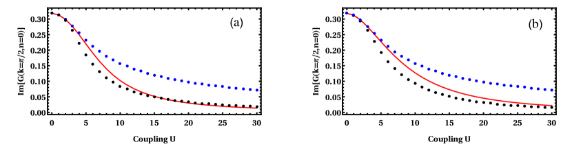
Figure 2: Comparison of GW, covariant quartic approximation and exact result for imaginary part of the Green function of 1D Hubbard model for (a)$T=1$,$\delta\mu=0$ and (b)$T=1$,$\delta\mu=0.2U$. The red line is the exact correlator, while blue and black dots are GW and CQA respectively.

V.4 Comparison with exact diagonalization (2D)

We calculated Green’s function of 2D Hubbard model, with $N=4$ and $T=1$ at half filling, for which reliable Monte Carlo simulations exist. The CQA and Monte Carlo results are shown in Fig.3. For $U\leq 2$ and $U\geq 12$ CQA results are in perfect agreement with QMC results.

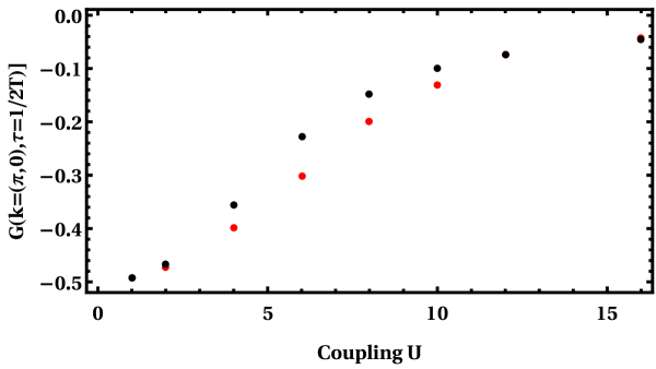
Figure 3: Green’s function $G(\mathbf{k},\tau)$ of a half filled 2D Hubbard model at $\mathbf{k}=(\pi,0)$ and $\tau=1/(2T)$. The red dots are MC result and the black ones are CQA result.

VI Estimate of complexity of the CQA computation

VI.1 Complexity of general calculation

In this section we estimate the complexity of a realistic strongly coupled condensed matter physics model computation using the Hubbard model as a representative example. Generalization to other models is briefly discussed in the concluding Section. It is convenient to consider the chain functions as a (spin/charge/band) vector $C_{\alpha\beta}^{f}$, since the most computationally intensive part of the computation is the chain equations iteration. For example in the single band Hubbard model the diffuson and the cooperon chains can be combined as:$C_{\alpha\beta}^{l}=\left\{d_{\alpha\beta}^{1},d_{\alpha\beta}^{2},c_{\alpha\beta},r_{\alpha\beta}\right\}$.The computation process is shown in Fig.4, where $\varepsilon=10^{-7}$ and $\epsilon=10^{-6}$, which leads to the deviation of the Green function solution less than $0.01\%$.

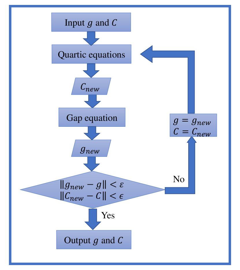
Figure 4: Flow chart of CQA calculation

Although in the simplest one band local Hubbard model the “channel” index $l$ takes $L=4$ values, the number $L$ becomes larger in multi - band Hubbard model or $t-J$ modelDagotto (1994); Scalapino (2012); Fradkin (2013). The frequency, quasi-momentum index, $\alpha=\left\{\omega,k_{1},...,k_{D}\right\}$, takes

$$n=2M_{{}^{\Omega}}N^{D}$$ (105)

values. In addition to chains one also iterates much smaller set of correlators $g_{\alpha}$. Generally the iteration of $C_{\alpha\beta}^{l}$ involves convolutions of $g$ and $C$ described in detail in Section V.

The computational cost of one iteration is estimated as follows. Computation for fixed $\beta$ and $L$ consists of roughly $L$ times convolutions implemented for example in MKLMKL (2019) (that as is done using fast Fourier transform and require $n\log\left[n\right]$ operations eachPress et al. (2007)). Different $\beta$ are computed in parallel. For a cluster with number of cores $N_{cores}<n$, the calculation time therefore can be estimated as

$$C=\frac{Ln^{2}}{N_{cores}}\log\left[n\right].$$ (106)

VI.2 Our calculation

In our $D=2$ sample computation for the simplest model described above one has: $L=4,$ $M_{{}^{\Omega}}=128,$ $N=4$ so that $n=256\times 4^{2}=4096$. The frequency cutoff $M_{{}^{\Omega}}$ is sufficient to simulate a relatively large temperature $T=t$. For the hopping parameter $t=0.4eV$ this amount to $4600K$. More relevant temperature range of $100-1000K$ will require larger $M_{{}^{\Omega}}$. To determine frequency cutoff at any temperature and coupling the convergence of $M_{{}^{\Omega}}\rightarrow\infty$ was studied. The energy cutoff ($M_{{}^{\Omega}}T$) should be larger than relevant energy scales: band width (hopping energy) and the on site Coulomb repulsion energy $U$ (coupling). The frequency cutoff is therefore estimated as,

$$M_{{}^{\Omega}}=8T^{-1}\max\left[2t,U/2\right]\text{.}$$ (107)

The present work uses $N_{cores}=32$ cores on the High-performance Computing Platform of Peking University. The equation Eq.(106) thus amounts to $C=\frac{4\times 4096^{2}}{32}\log\left[4096\right]=2\times 10^{7}$ operations per iteration. At not very large coupling used for the present exploratory calculation  (largest coupling to temperature ratio $U/T=30$) the number of iterations required for convergence $N_{it}$ scales with $U$ as

$$N_{it}=10U/T.$$ (108)

In our calculation each iteration took $16$ seconds, and 30 values of coupling $U=1,2,\cdots,30$ for a single value of temperature and frequency cutoff were calculated, it over all took 21 hours.

For a realistic applications(still in 2D but for a several band Hubbard type model and quasi - local interactions and higher values of coupling), more powerful computational resources are required.

VI.3 An estimate for a realistic 2D system.

For a more realistic applications one uses room temperature $T=300K$ (sometimes below for example when high $T_{c}$ superconductivity is considered the relevant range is below $100K$). Therefore it is feasible to perform calculation for strong coupling $U/T=80$ required for $T=0.1t$.

For a popular 3 band Hubbard model with several couplings considered to realistically describe perovskite 2D materialsDagotto (1994); Scalapino (2012) number of channels is about $L=10$. The values of the hopping parameter is about $t=0.25eV$ and the typical coupling strength $U=8t$. According to estimate Eq.(107) $M_{{}^{\Omega}}=32t/T=320$. Monte Carlo simulations at half filling  demonstrate that the continuum limit in this case is achieved for $N_{s}=12$. The number of cores available in Normal Taiwan University is $N_{cores}=1080$. The number of “degrees of freedom” is consequently $n=1\times 10^{5}$. According to the estimate Eq.(106), the one iteration time is determined by $C=\frac{10\times\left(1\times 10^{5}\right)^{2}}{1080}\log\left[1.\times 10^{5}\right]=1.5\times 10^{9}$ operations. This amounts to $33$ minutes.

The maximal number of iterations required estimates $N_{it}=10\times 80=800$ . The computation of the two - body correlator will take two weeks.

VII Discussion and conclusions

To summarize, we have developed a non - perturbative manifestly charge conserving method, covariant quartic approximation, determining the excitation properties of crystalline solids. It was shown that truncations of the set of Dyson - Schwinger equations for correlators of the downfolded model of materials lead to a converging series of approximants. The covariance ensures that all the Ward identities expressing the charge conservation are obeyed. A large number of solvable bosonic and fermionic field theoretical models demonstrate that the approximant in this series, is sufficiently precise. We focus here on the electron correlators describing single electron (hole) excitations observed directly by for example the photo-emission experiments.

The scheme was implemented on supercomputer and tested on the one band Hubbard model in both 1D (where exact diagonalization results were derived) and 2D at half filling (where determinantal quantum Monte Carlo results existBlankenbecler et al. (1981); Hirsch (1985); Santos (2003); Ma et al. (2013, 2018)). Estimates of the complexity for more realistic lattice models like local multi - band Hubbard were made.

The method is applicable in cases where various Monte Carlo based methods fail due to the sign problemBecca and Sorella (2017). In most cases of interest the sign problem therefore does not allow simulation. When comparing the two approaches in the absence of the sign problem (like in the half filled Hubbard model), note that the value of the frequency cutoff used in quartic approximation is much larger than the corresponding value used in MC simulations to achieve same precision. The MC estimate of the cutoff is $M=T^{-1}\sqrt{8tU}$, where $U$ is strength of interactions, $t$ is hopping parameter (band width for narrow bands)  and $T$ is temperature. This should be compared with our estimate in Eq.(107).

For realistic applications to strongly correlated electronic systemsFradkin (2013), more complicated models on the “mesoscopic scale” should be considered. Although the basic band structure of crystalline solids can be theoretically investigated by the density functional methods, the condensed matter characteristics dependent on the detailed structure of the electronic matter near the Fermi level requires more precise treatment of the relevant degrees of freedom conveniently represented as an “effective” lattice model on the scale of nanometer often taking the form of the local multi - band Hubbard model or a quasi - local $t-J$ model. Like some other methods for example versions of GW Aryasetiawan and Gunnarsson (1998), various Monte Carlo based methods like DMFTKotliar et al. (2006), FLEXBickers et al. (1989); Rohringer et al. (2018) and parquetteRubtsov et al. (2012); Astretsov et al. (2019), CQA therefore can also be applied to the effective lattice models with pairwise interactions.