The first observed stellar occultations by the irregular satellite red(Saturn IX) Phoebe and improved rotational period

Abstract

We report six stellar occultations by red(Saturn IX) Phoebe, an irregular satellite of Saturn, obtained between mid-2017 and mid-2019. The 2017 July 06 event is the first stellar occultation by an irregular satellite ever observed. The occultation chords were compared to a 3D shape model of the satellite obtained from Cassini observations. The rotation period available in the literature led to a sub-observer point at the moment of the observed occultations where the chords could not fit the 3D model. A procedure was developed to identify the correct sub-observer longitude. It allowed us to obtain redthe rotation period with improved precision redover currently known value from literature. We show that the difference between the observed and the predicted sub-observer longitude suggests two possible solutions for redthe rotation period. By comparing these values with recently observed rotational light curves and single-chord stellar occultations, we can identify the best solution for Phoebe’s rotational period as red$9.27365\pm 0.00002$ h. From the stellar occultations, we also obtained 6 geocentric astrometric positions in the ICRS as realised by the Gaia-DR2 with uncertainties at the 1-mas level.

1 Introduction

Phoebe is the first irregular satellite to be discovered, in 1898, by William Henry Pickering (Pickering, 1899). It is also the first object to be identified with a retrograde orbit by Ross (1905). Until the year 2000, it was the only known Saturnian irregular satellite (Gladman et al., 2001).

Phoebe is the only irregular satellite to have been visited by a spacecraft. The visit was made by the Cassini-Huygens Spacecraft in 11 June 2004 (Porco et al., 2005), which observations resolved the shape of the object. Unfortunately, since it was a quick flyby, not all regions of Phoebe were observed. The maximum resolution of Cassini observations was 13 m px^-1, however, as can be seen in Porco et al. (2005), the resolution varies a lot depending on the latitude and longitude of Phoebe. In particular, the region close to the North Pole (latitudes higher than $+60\degr$) was always in the dark, and it was not imaged. An important point is that, during 2017-2019, the north region is visible from Earth.

From Cassini observations, Thomas (2010) determined the semi-axis of Phoebe as a=$109.4\pm 1.4$ km, b=$108.5\pm 0.6$ km and c=$101.8\pm 0.3$ km. Considering the error bars of $a$ and $b$, Phoebe can be considered as an oblate spheroid.

Due to its orbital characteristics, it is believed Phoebe has been captured by Saturn during the evolution of the Solar System. This assumption is supported by Cassini observation showing that Phoebe must have a composition different from other Saturnian satellites (Johnson & Lunine, 2005). Clark et al. (2005) concluded that Phoebe has a surface that is covered by material of cometary or outer Solar System origin.

The technique of stellar occultation, which can achieve kilometre accuracy (e.g. Braga-Ribas et al., 2014), can be used to constrain the shape of Phoebe in the regions that were not observed by Cassini. Since Phoebe’s pole coordinates and rotational period are known, it is possible to associate the occultation chords with a specific latitude and longitude on Phoebe’s surface.

In this regard, Gomes-Júnior et al. (2016) predicted stellar occultations by Phoebe up to 2020. They showed that Saturn was crossing a region on the sky that had the Galactic Plane as background by the end-2017 and 2018, increasing the number of predicted events by a factor of 10. To have good predictions, the ephemeris of Phoebe was improved by using all observations available.

The first observed stellar occultation by Phoebe occurred in 2017 July 06. This occultation was observed in Japan by two sites. In 2018, other four occultations were observed, in South America (June 19) and Australia (June 26, July 03 and August 13). The sixth one was observed in 2019 June 07 in South America. Only the first occultation was multi-chord.

The observations details are presented in section 2 and the occultation light curves are described in section 3. In section 4, we show the reduction process of the two chords of the 2017 July 06 event comparing them with a 3D shape model. In section 5 we discuss the improvement of the rotation model of Phoebe from the occultations results. In section 6 we discuss over the 2018 and 2019 events and how they could help to improve Phoebe’s rotation period. In section 7 we compare our solutions to a rotational light curve of Phoebe. The results are presented in section 8. The conclusion and final remarks are set in section 9.

2 Predictions and Observations

The predictions for all the events were first made by Gomes-Júnior et al. (2016) with UCAC4 stars (Zacharias et al., 2013). We then updated the star positions with newer catalogues as the occultation epoch approached. The first occultation by Phoebe was observed in 2017 July 06, which star position was updated using Gaia-DR1. Since the star was also a Tycho-2 star (TYC 6247-505-1), we benefited of the Tycho-Gaia Astrometric Solution (TGAS, Michalik et al., 2015), with proper motions and parallax, deriving a better position than most of the Gaia-DR1 stars.

In 2018 April, Gaia-DR2 was published (Brown et al., 2018), so the next candidate stars’ positions were updated allowing accurate predictions and the observation of five more occultations. For the fitting procedure, the Gaia-DR2 star positions were used for all six events. Table 1 shows the geocentric ICRS coordinates of the stars at the occultation epoch, corrected from proper motion, parallax and radial velocity. The catalogued G magnitude of the stars are presented, which can be compared to Phoebe’s V=16.6.

Table 1: Occulted star parameters for each event.

Occ. Date	Gaia DR2 star designation	G Mag	Right Ascension ($\alpha$)*	Declination ($\delta$)*	Diam.** (km)
2017 July 06	4117746607441803776	10.3	17h 31m 03$\aas@@fstack{s}$03947 $\pm$ 0.2 mas	-22°00′58$\aas@@fstack{\prime\prime}$0938 $\pm$ 0.2 mas	1.18
2018 June 19	4090124156586307072	14.9	18h 26m 16$\aas@@fstack{s}$40061 $\pm$ 0.4 mas	-22°24′00$\aas@@fstack{\prime\prime}$4378 $\pm$ 0.3 mas	0.15
2018 June 26	4089759672845036416	14.4	18h 24m 01$\aas@@fstack{s}$50061 $\pm$ 0.2 mas	-22°26′12$\aas@@fstack{\prime\prime}$1804 $\pm$ 0.2 mas	0.19
2018 July 03	4089802618196107776	15.6	18h 22m 00$\aas@@fstack{s}$25777 $\pm$ 0.3 mas	-22°28′10$\aas@@fstack{\prime\prime}$7057 $\pm$ 0.3 mas	0.24
2018 Aug 13	4066666389602814208	17.5	18h 12m 22$\aas@@fstack{s}$37073 $\pm$ 0.6 mas	-22°38′44$\aas@@fstack{\prime\prime}$2087 $\pm$ 0.6 mas	0.14
2019 June 07	6772694935064300416	15.3	19h 21m 18$\aas@@fstack{s}$63201 $\pm$ 0.3 mas	-21°44′25$\aas@@fstack{\prime\prime}$3924 $\pm$ 0.3 mas	0.10

*Gaia-DR2 star position at the time of occultation. **Apparent star diameter at the distance of Phoebe.

The positions of Phoebe were determined from the ephemeris published by Gomes-Júnior et al. (2016), PH15, and the planetary ephemeris JPL DE438. PH15 is an updated version of PH12 published by Desmars et al. (2013).

Figure 1 shows the post-reduction occultation maps. redThe typical difference between the predicted and observed occultations was smaller than Phoebe’s radius. It also shows the location of the sites that attempted to observe the events. In green we have the sites where the occultation was positive, in red the sites with no detection, and in white the site whose observation should be positive, but the low signal-to-noise ratio (SNR) in combination with a long exposure did not allowed the detection of the occultation. Table 2 shows the circumstances of the observations, telescopes and detector used for each site on each event.

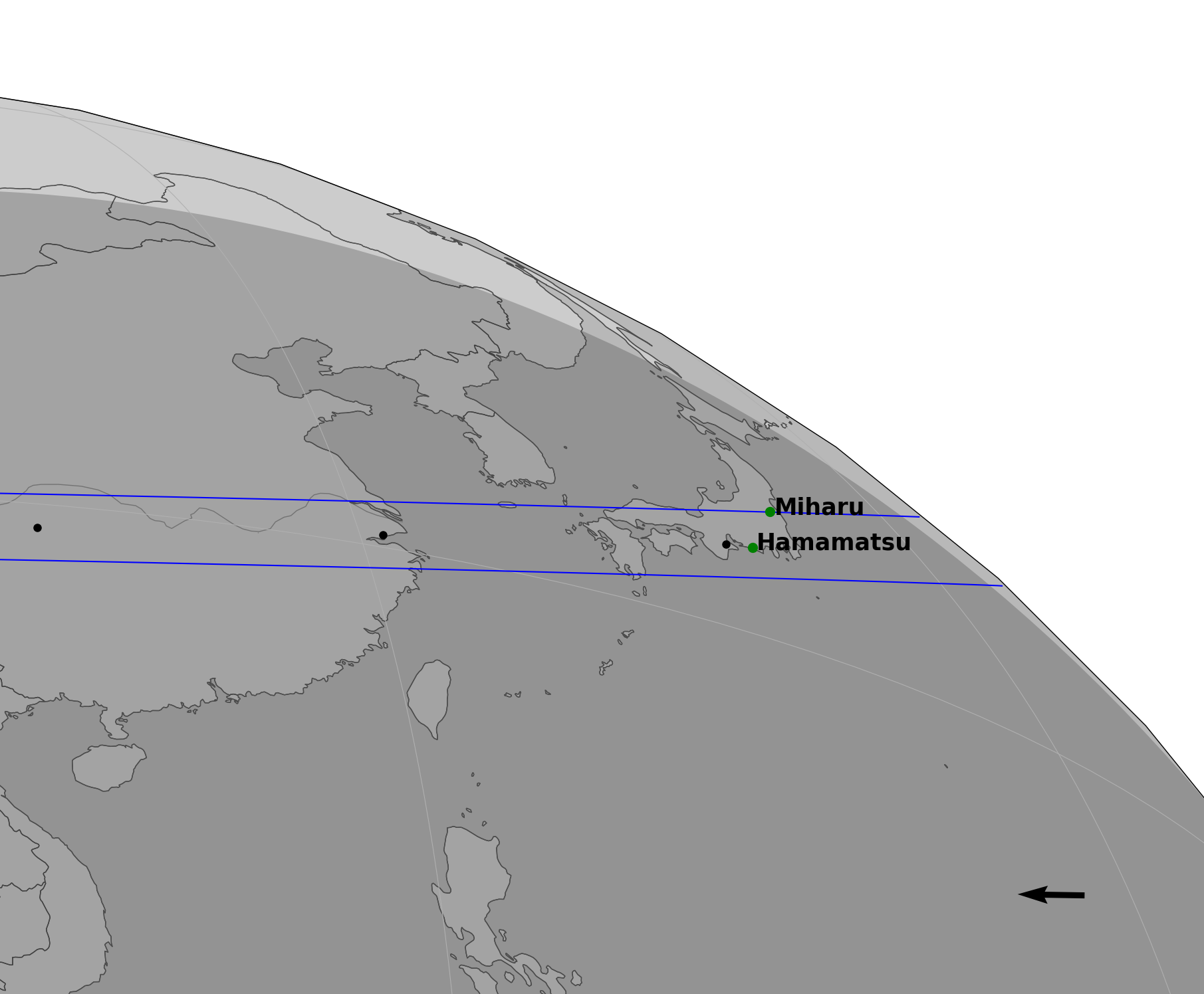
(a) 2017 July 06

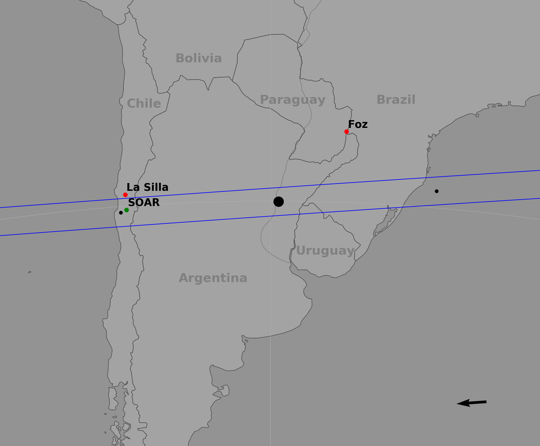
(b) 2018 June 19

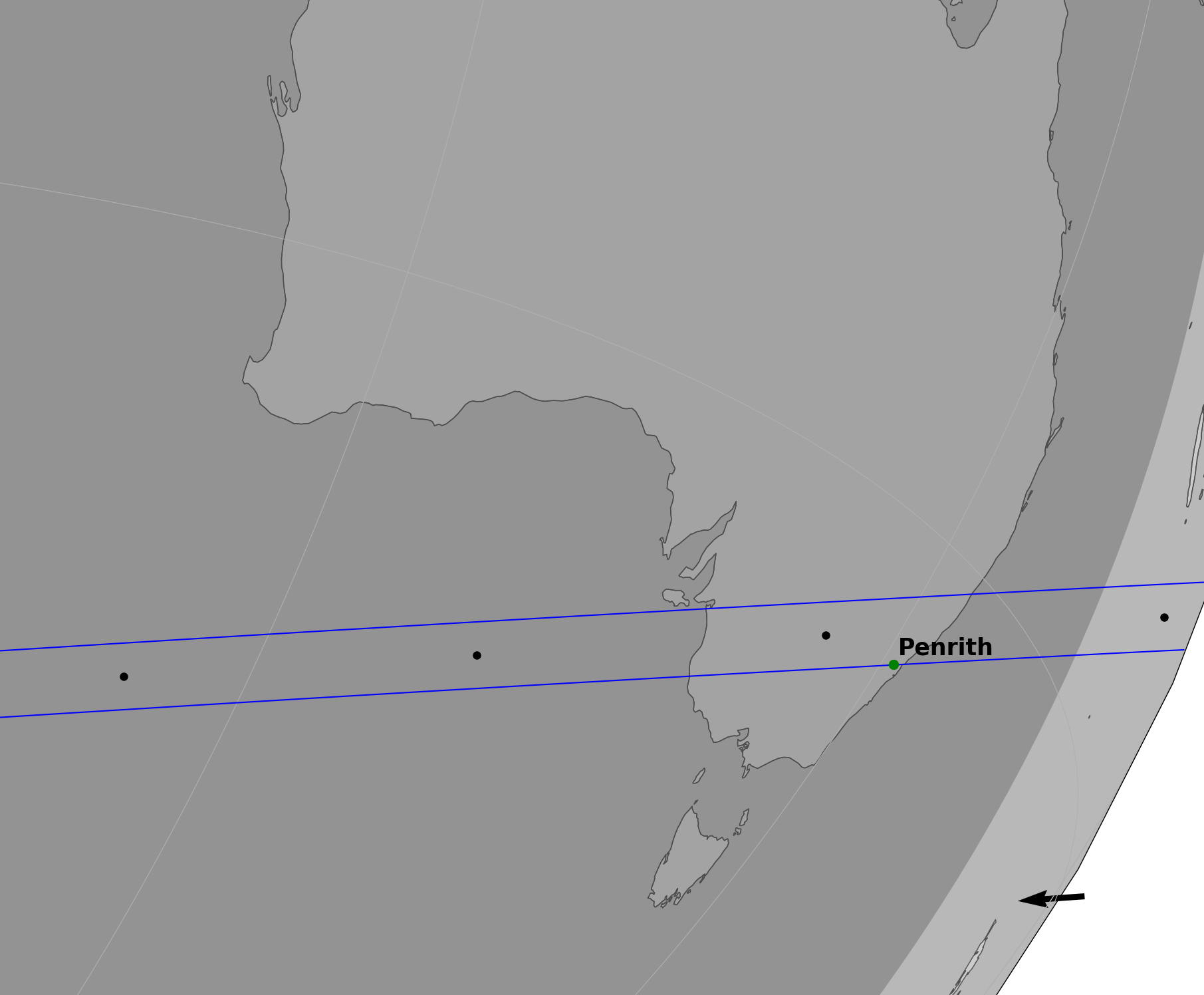
(c) 2018 June 26

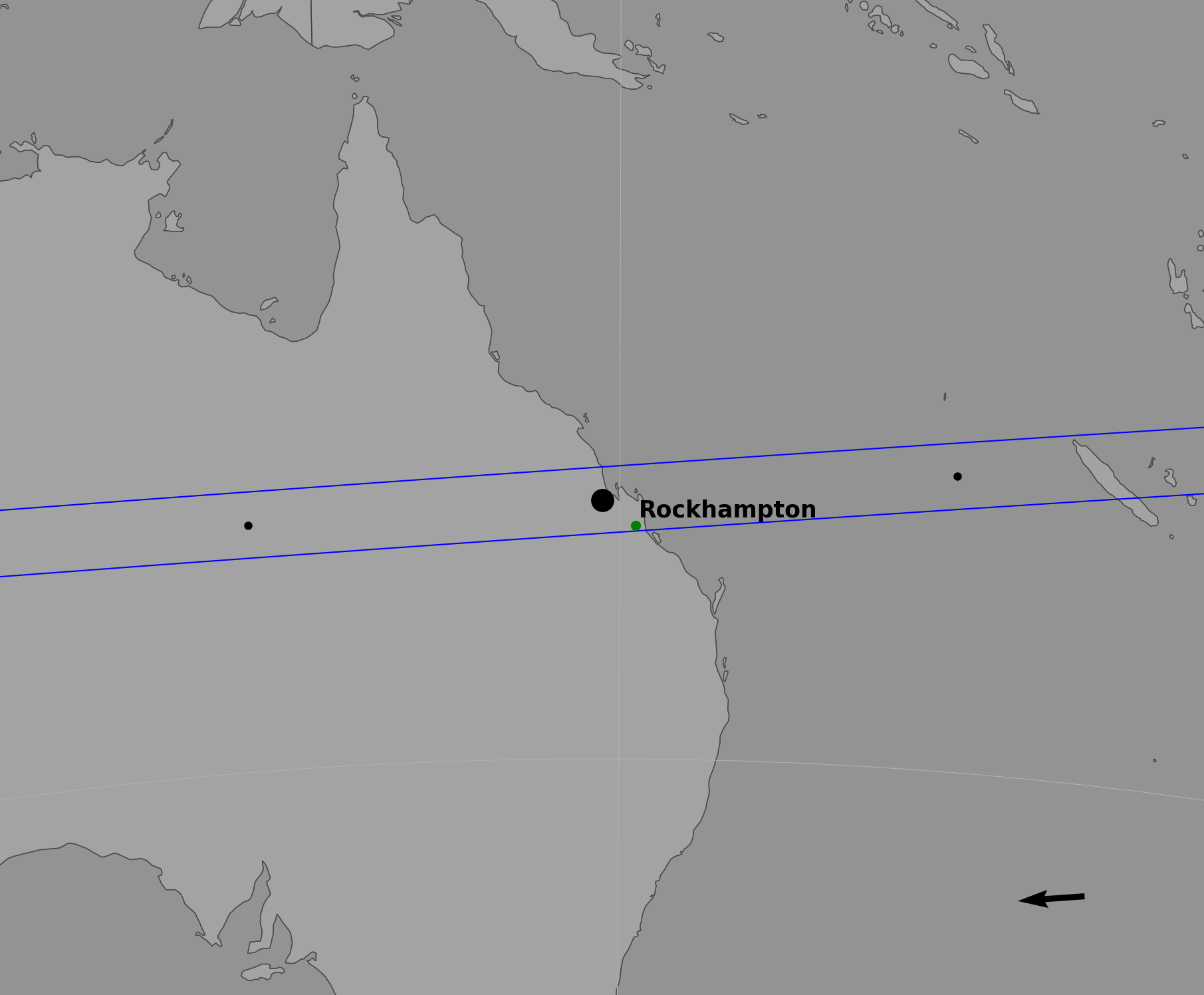
(d) 2018 July 03

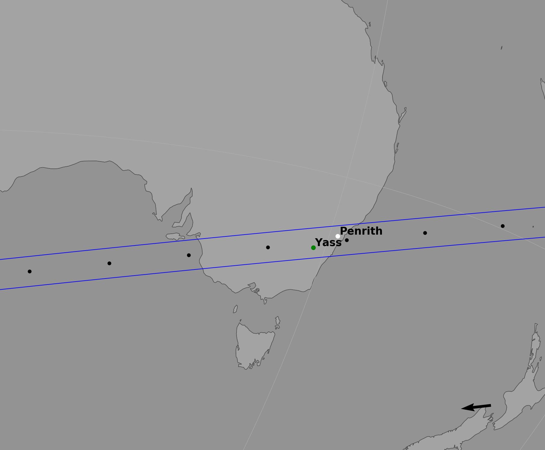
(e) 2018 August 13

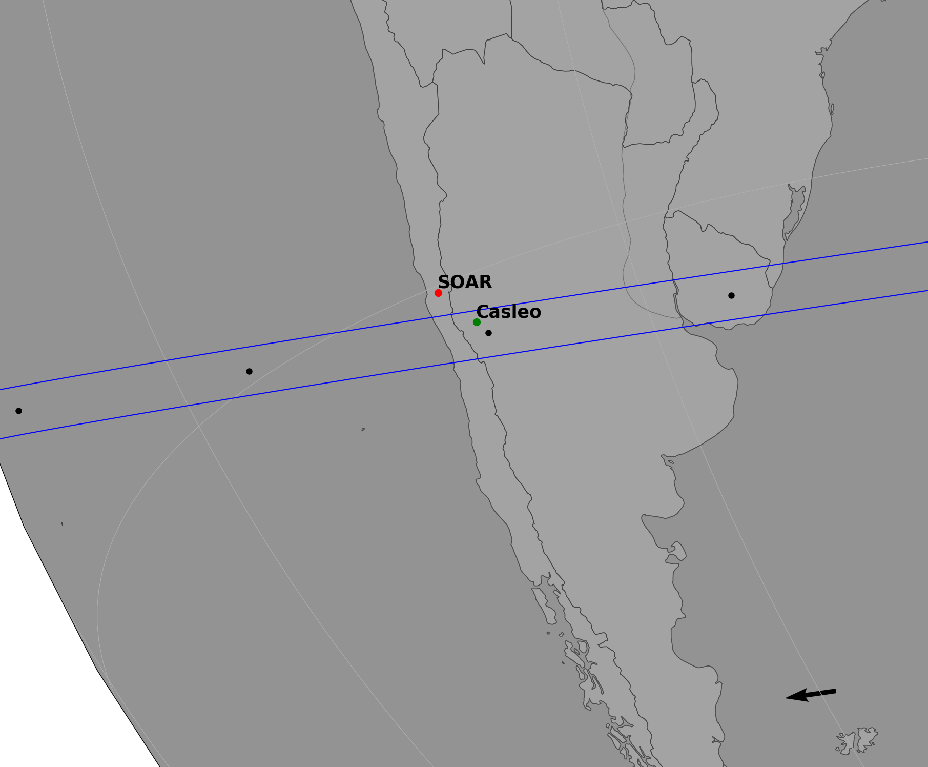
(f) 2019 June 07

Figure 1: Post-fit maps of Phoebe’s occultations. The green dots are the sites that got a positive detection, while the red ones are sites where the detection was negative. The white dot site on the August 13 occultation (e) observed the occultation but with a very low SNR. The blue lines show the path of the shadow with the projected diameter of Phoebe. The black dots show the centre of the shadow separated by one minute. redThe big black dots show the position of the shadow for the geocentric closest approach between satellite and star. The arrows on the right low corner show the direction of the shadow’s movement.

Table 2: Circumstances of observation for all observing stations.

	Longitude	Telescope	Camera	Detection
Site	Latitude	Aperture	Exp/Cycle time	Ingress	Observers
	Altitude	f-ratio	Time-Stamp	Egress
2017 July 06
Hamamatsu	137°44′23$\aas@@fstack{\prime\prime}$0 E	Schmidt Cass	WAT-120+	Positive	Minoru Owada
Japan	34°43′07$\aas@@fstack{\prime\prime}$0 N	25 cm	0.534 s	16:03:59.55$\pm 0.04$ s
	17 m	f/9.3	GHS-OSD	16:04:11.03$\pm 0.04$ s
Miharu	140°26′04$\aas@@fstack{\prime\prime}$2 E	Newtonian	WAT-120	Positive	Katsumasa Hosoi
Japan	37°25′36$\aas@@fstack{\prime\prime}$7 N	13 cm	0.534 s	16:04:00.83$\pm 0.1$ s
	274 m	f/5	GHS-OSD	16:04:02.07$\pm 0.1$ s
2018 June 19
Cerro Pachon	70°44′21$\aas@@fstack{\prime\prime}$7 W	SOAR	Raptor	Positive	J. I. B. Camargo
Chile	30°14′16$\aas@@fstack{\prime\prime}$9 S	420 cm	0.2 s	04:37:49.844 $\pm$ 0.009 s	A. R. Gomes Júnior
	2693.9 m	f/16	GPS	04:38:01.343 $\pm$ 0.007 s
La Silla	70°44′20$\aas@@fstack{\prime\prime}$18 W	Danish	Lucky Imager	Negative	Justyn Campbell-White
Chile	29°15′21$\aas@@fstack{\prime\prime}$27 S	154 cm	0.1 s	beg: 04:35:01.05	Sohrab Rahvar
	2336 m	f/8.6	GPS-connected NTP	end: 04:41:14.07	Colin Snodgrass
La Silla	70°44′21$\aas@@fstack{\prime\prime}$8 W	TRAPPIST-S	FLI PL3041-BB	Negative	Emmanuel Jehin
Chile	29°15′16$\aas@@fstack{\prime\prime}$6 S	60 cm	3.0/4.13 s	beg: 04:24:01.82
	2317.7 m	f/8	NTP	end: 04:47:19.71
Foz do Iguaçu	54°35′37$\aas@@fstack{\prime\prime}$50 W	Celestron	Raptor	Negative	Daniel I. Machado
Brazil	25°26′05$\aas@@fstack{\prime\prime}$36 S	28 cm	5.0 s	beg: 04:31:32.15
	184.8 m	f/10	GPS180PEX, Meinberg	end: 04:46:27.15
2018 June 26
Penrith Obs.	150°44′29$\aas@@fstack{\prime\prime}$9 E	Ritchey-Chretien	Grasshopper Express	Positive	Tony Barry
Australia	33°45′43$\aas@@fstack{\prime\prime}$5 S	60 cm	1.0 s	18:31:20.1 $\pm$ 0.1 s	Ain De Horta
	58 m	f/10	ADVS	18:31:21.3 $\pm$ 0.1 s	David Giles
					Rob Horvat
2018 July 03
Rockhampton	150°30′01$\aas@@fstack{\prime\prime}$6 E	SCT	Watec 910BD	Positive	Stephen Kerr
Australia	23°16′10$\aas@@fstack{\prime\prime}$1 S	30 cm	1.28 s	13:37:51.8 $\pm$ 0.2 s
	50 m	f/10	IOTA-VTI	13:37:56.9 $\pm$ 0.2 s
2018 August 13
Yass	148°58′35$\aas@@fstack{\prime\prime}$14 E	Planewave CDK20	QHY174M-GPS	Positive	William Hanna
Australia	34°51′51$\aas@@fstack{\prime\prime}$17 S	50.8 cm	2.0 s	12:52:45.3 $\pm$ 0.7 s
	535 m	f/4.4	in-camera GPS	12:53:08.1 $\pm$ 0.7 s
Penrith Obs.	150°44′29$\aas@@fstack{\prime\prime}$9 E	Ritchey-Chretien	SBIG STT-8300	Bad SNR	Tony Barry
Australia	33°45′43$\aas@@fstack{\prime\prime}$5 S	60 cm	8.0/9.0 s	beg: 12:31:53.0	Ain De Horta
	58 m	f/10	NTP	end: 12:54:32.0	David Giles
					Rob Horvat
					Darren Maybour
2019 June 07
Casleo	69°17′44$\aas@@fstack{\prime\prime}$9 W	Jorge Sahade	Versarray 2048B, Roper Scientific	Positive	Luis A. Mammana
Argentina	31°47′55$\aas@@fstack{\prime\prime}$6 S	215 cm	0.5/2.0 s	03:54:22.6 $\pm$ 0.9 s	Eduardo F. Lajús
	2552 m	f/8.5	GPS	03:54:32.5 $\pm$ 0.6 s
Cerro Pachon	70°44′21$\aas@@fstack{\prime\prime}$7 W	SOAR	Raptor	Negative	J. I. B. Camargo
Chile	30°14′16$\aas@@fstack{\prime\prime}$9 S	420 cm	0.4 s	beg: 03:48:44.4	A. R. Gomes Júnior
	2693.9 m	f/16	SOAR	end: 04:05:02.8

Details about the Danish instrument can be found in Skottfelt et al. (2015) and for the TRAPPIST one in Jehin et al. (2011).

Many of the observations were made using video cameras. The procedures of the reduction of video observations are similar to those used by Benedetti-Rossi et al. (2016). Each individual frame from the video is converted to FITS format, with a frame rate used by the observer, using our own code which uses astropy and ffmpeg features. All frames were checked to verify the presence of duplicated fields or missing frames in the data set.

To recover the individual exposure of each observation, for example the 0.534 second observed in the 2017 event, a group of frames corresponding to the same exposure was considered, with the first and last frames of each sequence being removed to avoid interlace problems between different exposures. The average of the remaining frames was obtained to represent an individual image. The mid-exposure time of each image was verified by comparing the extracted time to the time printed on the frames of the video, given by a video time inserter. For a better understanding of the procedure, refer to Benedetti-Rossi et al. (2016).

3 Light Curve Reduction

For each observation, the flux of the occulted star was determined by a differential aperture photometry using the Package for Reduction of Astronomical Images Automatically (praia, Assafin et al., 2011). The light curve obtained was calibrated and normalised by the flux of a calibration star. The final light curves from all positive observations are shown in Figure 2.

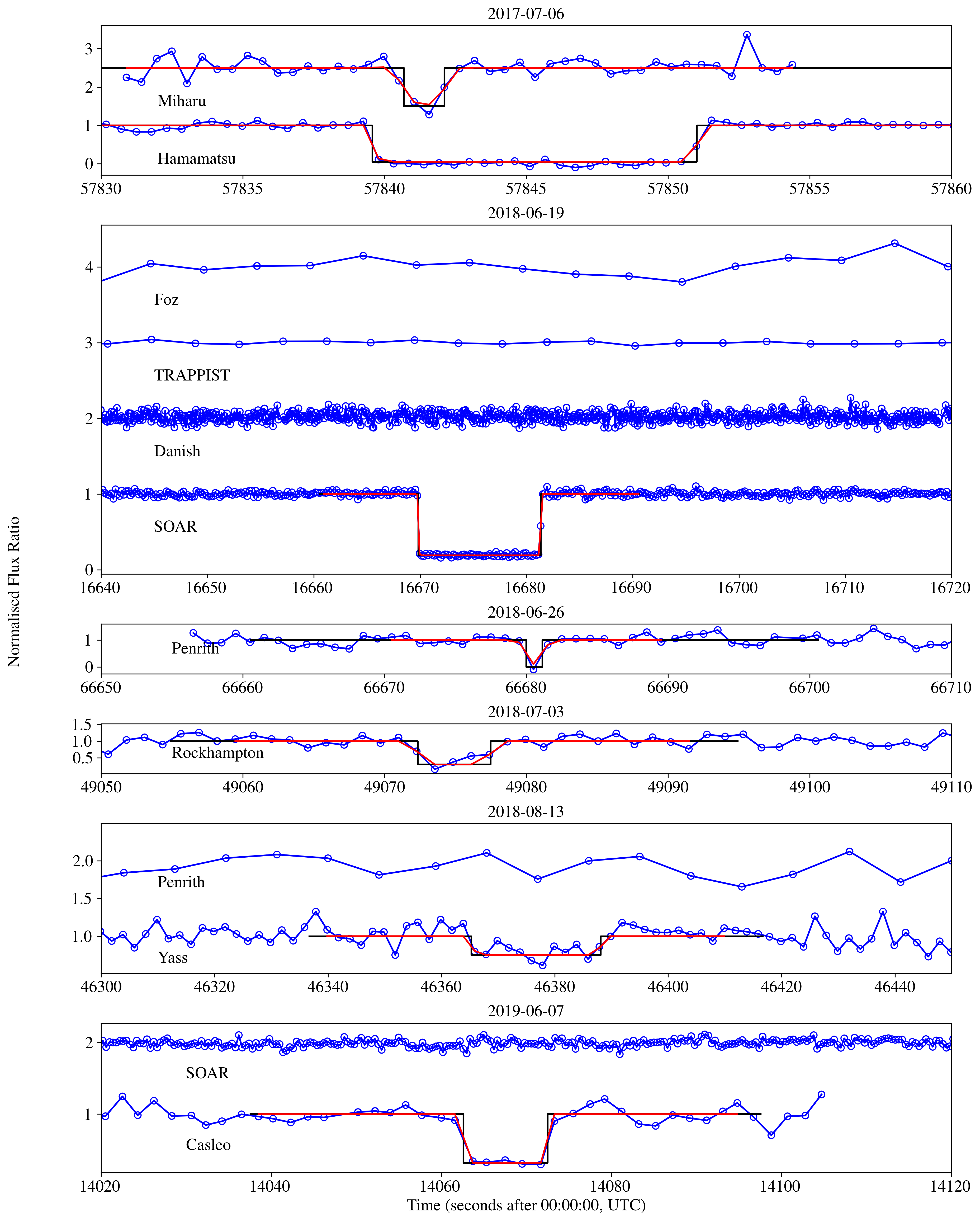
Figure 2: Normalised light curves from the six stellar occultations by Phoebe. Some curves are vertically shifted for better visualisation. The blue lines show the normalised flux ratio of Phoebe plus occulted star relative to the calibration star. The solid black lines are the best fit of the square-well model to the data. Red lines are the square-well model convoluted with the Fresnel diffraction, the star diameter, and the applied exposure time.

The procedure of determination of the instants of ingress (disappearance) and egress (reappearance) in the light curves is similar to the one adopted by Braga-Ribas et al. (2013), where a square-well model is convoluted with the Fresnel diffraction, the CCD bandwidth, the stellar apparent diameter, and the applied finite exposure time.

From the diameter and parallax of the stars given by Gaia-DR2 (Andrae et al., 2018) we determine the diameter projected at Phoebe’s distance for the 2017 and 2019 events. For the remaining, the diameter was estimated with the formulae of van Belle (1999) by using the magnitudes found in the literature. These values are given in Table 1. The Fresnel scale was between 0.714-0.721 km. For all observations, those effects are negligible compared to the length corresponding to one exposure, thus this last being the main parameter in the determination of the instants of star disappearance (ingress) and reappearance (egress) of the light curves.

The fitting process consists in minimising a classical $\chi^{2}$ function for each light curve, where the free parameter is the ingress or egress instant. Figure 2 shows all the observed light curves with the corresponding model in red. The ingress and egress instants obtained and respective uncertainties, at 1-$\sigma$ level, are shown in Table 2. For the 2018 August 13 event, the Penrith Observatory is on the shadow path, however, due to the observation conditions, the SNR was too small and the flux drop could not be identified.

4 The 2017 July 06 occultation

Since Phoebe already has a known shape from Cassini observations, we used the 3D model of Gaskell (2013) to fit our chords. As shown by Cassini, Phoebe is highly cratered, with the largest one having an estimated size of $\sim 100$ km (Porco et al., 2005), with walls that can reach 15 km high, which is significant relative to Phoebe’s size. So it is likely that both chords encompass topographical features.

The sub-observer latitude ($\phi$) and longitude ($\lambda$) at the instant of observation (16:04:00 UTC) was determined from Archinal et al. (2018) as $\phi=22.3\degr$ and $\lambda=330\degr$. From the pole coordinates of Phoebe red($\alpha_{p}=356.90\degr$, $\delta_{p}=77.80\degr$), given by Archinal et al. (2018), and its ephemeris at the mid-instant of the occultation, from Gomes-Júnior et al. (2016), we determined the pole position angle as $PA=13.2\degr$.

Figure 3 shows the fit from the chords to the 3D shape model of Phoebe using the presented orientation. It is possible to see that the Miharu chord is close to the North Pole of the object. In green, the limb of Phoebe projected on the sky plane is highlighted. The centre was determined by fitting the Hamamatsu chord. Since it is in a central region, this chord is expected to be located in a region that was better observed by Cassini than Miharu’s. The surface brightness texture presented in the image comes from Cassini observations given by Gaskell (2013). The regions in black were not observed by Cassini or were always in darkness.

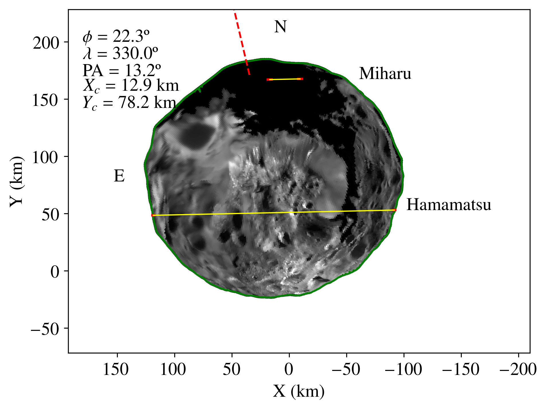
Figure 3: Fit of the two chords from the 2017 July 06 occultation to the 3D shape model of Phoebe given by Gaskell (2013). The sub-observer latitude $\phi$ and longitude $\lambda$ was calculated from the rotation model of Archinal et al. (2018). $PA$ is the position angle of the north pole of Phoebe. $X_{c}$ and $Y_{c}$ are the coordinates of the centre of Phoebe relative to the prediction, taking the star coordinates from Gaia DR2. The yellow lines show the observed chords and the red segments show their error bars. The dashed red line shows the direction of the North Pole of Phoebe.

It is possible to see in Figure 3 that the Miharu chord is located very far from the projected limb of the 3D shape model, while the Hamamatsu chord fits very well. Regions observed by Cassini in the continuation of the chord were not detected in the occultation.

In preparation for the Cassini mission, Bauer et al. (2004) determined the rotational period of Phoebe redas $9.2735\pm 0.0006$ h. Propagating it from 2004 to the occultation time, it represents an uncertainty in the sub-observer longitude of $\pm 305\degr$. That means that the nominal sub-observer longitude calculated from Archinal et al. (2018) is probably wrong. Since the sub-observer latitude and position angle are better determined, the goal now is to determine the sub-observer longitude that better fits the 3D shape model and occultation chords.

To retrieve the correct sub-observer longitude, a $\chi^{2}$ analysis was done for all longitudes, ranging from $0\degr$ to $360\degr$ with a $0.5\degr$ step. Since the Hamamatsu chord probed the central region, where the 3D model has a better spatial resolution, only this chord was used to fit the object’s centre ($X_{c}$, $Y_{c}$). With this condition satisfied, we calculated the total $\chi^{2}$ with the chord extremities using Equation 1:

$$\chi^{2}=\sum\dfrac{(R_{c}-R_{l})^{2}}{\sigma^{2}}$$ (1)

where $R_{c}$ is the radial distance of each chord extremity from the geometric centre given by ($X_{c}$, $Y_{c}$) and $R_{l}$ is the radial distance of the limb of the 3D shape model at the same direction as $R_{c}$. The uncertainty $\sigma$ of each point was 0.7 km for Hamamatsu and 1.6 km for Miharu.

Figure 4 shows the distribution of $\chi^{2}$ by longitude. It is possible to see that the $\chi^{2}$ varies from almost zero up to 700. For comparison, in Figure 3 $\chi^{2}$ is equal to 201.

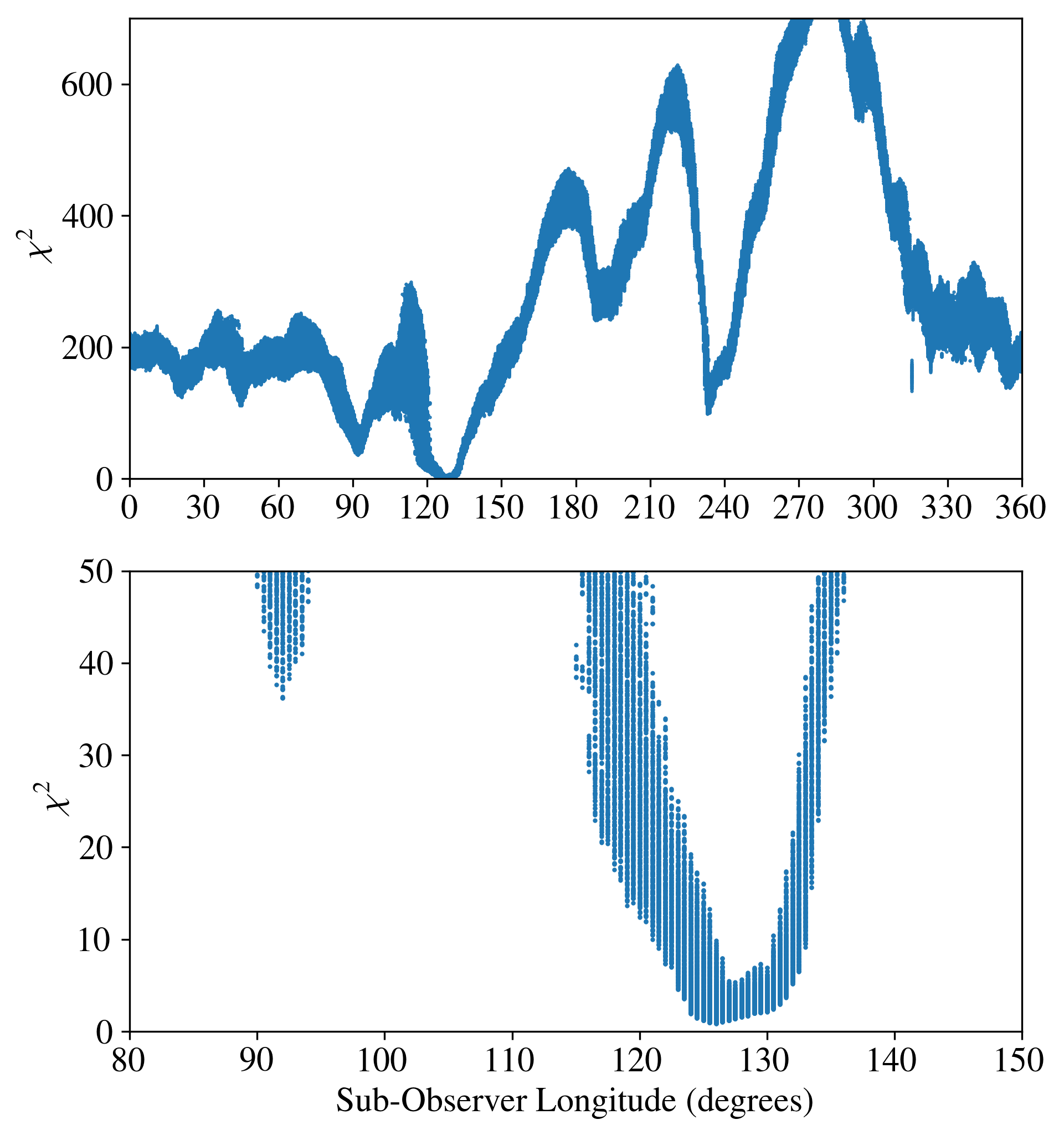
Figure 4: Distribution of $\chi^{2}$ over longitude (see discussion in section 4). Upper panel: chi-square over all longitudes. Bottom panel: zoom in the region of local minima.

Although the Miharu chord crosses a region that was not well observed by Cassini, it is expected the Gaskell (2013) shape model to be realistic enough considering the relatively higher error of this chord. Thus, it is difficult to establish which value of $\chi^{2}$ is acceptable. Because of this, we analyse the local minima presented in Figure 4.

The most prominent minimum is at the longitude $126.5\degr$ with a $\chi^{2}=0.85$. Figure 5 shows the best fit in this case. It is possible to see that the western contact point of Miharu chord seems to be in a region that was observed by Cassini, though it was a region observed in lower resolution. The second minimum in the Figure 4 is located at the longitude $92.0\degr$ with a $\chi^{2}=36.2$. Figure 6 shows the best fit in this case.

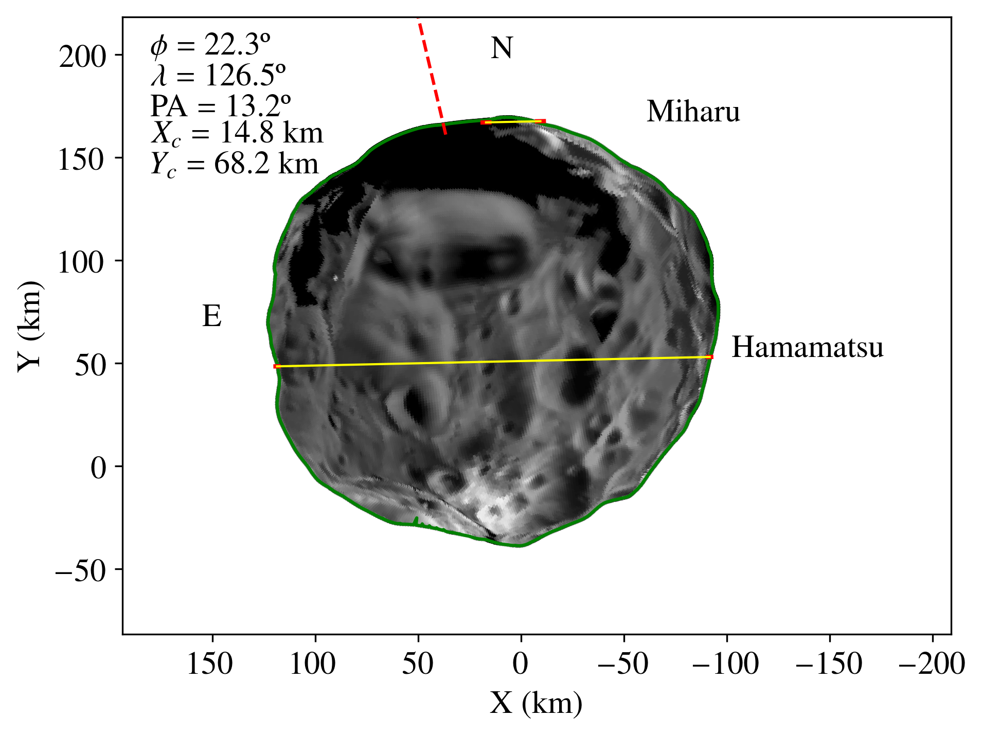
Figure 5: Similar to the Figure 3, but fitting the chords to the 3D shape model using the sub-observer longitude of $126.5\degr$.

In Table 3 we present the limits of values ($\lambda$, $X_{c}$, $Y_{c}$) within 1-$\sigma$ ($\chi^{2}_{min}+1$) for the two main chi-square minima of Figure 4. The radial residuals of the Miharu chord are also presented, separated by its western and eastern contact points. Thus, we can infer possible topographic characteristics, if any.

Table 3: Results of $\lambda$, $X_{c}$, $Y_{c}$ for the two chi-square minima of the Figure 4. Miharu W refers to radial residuals between the chord and the 3D model to the western contact point of the Miharu chord and Miharu E to the eastern contact point.

$\lambda$	$X_{c}$	$Y_{c}$	Miharu W	Miharu E
(°)	(km)	(km)	(km)	(km)
$126.5\pm 3.5$	$14.8\pm 0.7$	$68.2\pm 1.1$	$0.8\pm 1.2$	$-1.2\pm 1.0$
$92.0\pm 1.0$	$12.9\pm 0.2$	$73.0\pm 0.1$	$-4.9\pm 0.1$	$-8.2\pm 0.1$

The results of Table 3 show that for the $\lambda=126.5\degr$ solution the western contact point of the Miharu chord agrees with the projected limb of the 3D model, while the eastern contact point suggest a slight variation in the direction of the centre of the figure, that could be caused by a crater not taken into account in the shape model.

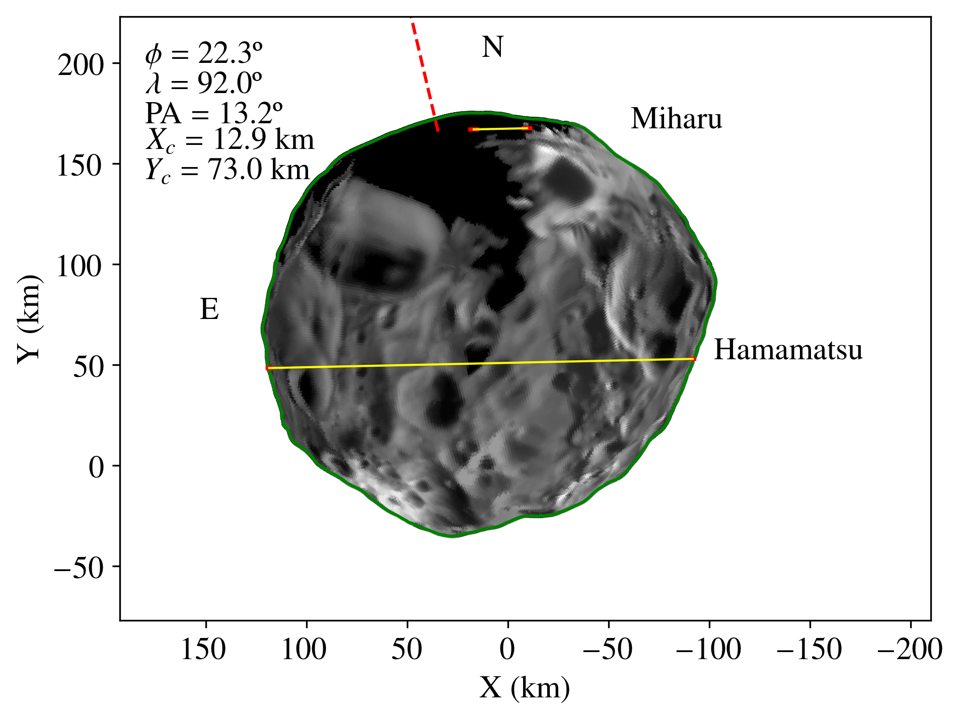
Figure 6: Similar to the Figure 3, but fitting the chords to the 3D shape model using the sub-observer longitude of $92\degr$.

In the case of $\lambda=92\degr$, the results suggest that both contact points of the Miharu chord would be in craters with 5 to 8 km of difference from the shape model of Gaskell (2013). Figure 6 shows that some regions observed by Cassini west of the chord should have been detected.

For other longitudes, the $\chi^{2}$ calculated are even less significant, meaning larger differences between the chords and the 3D model of Gaskell (2013). Because of this, it is not expected to find better results with other longitudes. Considering it all, the sub-observer longitude of $126.5\degr\pm 3.5\degr$ is chosen as our unique solution at the epoch of the 2017 July 06 occultation.

5 Improved rotational period

The rotation model of Phoebe from Archinal et al. (2018) predicts the sub-observer longitude at the time of the 2017 July 06 occultation as $\lambda=330.5\degr$. From the analysis in section 4, we identify a phase difference of $-204.0\pm 3.5\degr$ or $+156.0\pm 3.5\degr$, representing an error of about half a rotation. Both possibilities are inside the $\pm 305\degr$ sub-observer longitude error bar estimate from Archinal et al. (2018) at the occultation epoch.

From Archinal et al. (2018) we calculate the location of the prime meridian (the half great-circle connecting the body’s north and south pole defined as $\lambda=0\degr$ in the body-centred reference frame), using $W=178.58+931.639d$ ($W$ is the ephemeris position of the prime meridian and $d$ is the interval in days from J2000), at the epoch of the Cassini maximum approach ($W_{\text{cas}}$), where it has the smallest error (Thomas, 2018, priv. comm.), and the instant of occultation ($W_{\text{occ}}$). Then we apply the phase difference determined for $W_{\text{occ}}$ and, keeping $W_{\text{cas}}$ fixed, we fit new parameters.

For the phase difference of $-204.0\degr$ we obtain $W=247.92+931.5963d$, which means a rotational period of red$9.27440\pm 0.00002$ h. For the $+156.0\degr$ phase difference, we determine $W=125.56+931.6717d$ meaning a rotational period of red$9.27365\pm 0.00002$ h. We denominate these solutions as "W1" and "W2" respectively.

6 The 2018 and 2019 stellar occultations

In 2018 and 2019 five other stellar occultations by Phoebe were observed. Only one positive detection was obtained for each event. Because of this, it is not possible to confidently apply the procedure described in section 4. Even so, we still can analyse the possible solutions obtained in section 5 and constrain Phoebe’s positions.

We first determined the new longitudes of Phoebe in the direction of the observers for each occultation using the solutions obtained in section 5. These values are shown in Table 4. Then we fit the chords to the shape model using only the latitude, pole position angle and the 1-sigma interval of longitude to obtain all the possible $X_{c}$ and $Y_{c}$ relative to Gomes-Júnior et al. (2016) ephemeris. These values are also shown in Table 4.

Table 4: Results for the centre of Phoebe from the stellar occultations of 2018 and 2019. For each event the sub-observer longitude ($\phi$), the Position Angle (PA), the sub-observer longitude ($\lambda$) and the ephemeris offset ($X_{c}$, $Y_{c}$) are presented. The results are shown for both solutions of the rotation period described in section 5.

Date			W1 solution			W2 solution
	$\phi$ ($\degr$)	PA ($\degr$)	$\lambda$ ($\degr$)	$X_{c}$ (km)	$Y_{c}$ (km)	$\lambda$ ($\degr$)	$X_{c}$ (km)	$Y_{c}$ (km)
2018 June 19*	19.8	12.8	$225.5^{+2.5}_{-3.7}$	-45.5 $\pm$ 1.5	-25.0 $\pm$ 8.0	251.5 $\pm$ 3.7	-46.0 $\pm$ 1.0	-40.0 $\pm$ 3.0
2018 June 26	20.0	12.8	86.5 $\pm$ 3.7	-75.0 $\pm$ 6.5	-44.5 $\pm$ 1.5	112.5 $\pm$ 3.7	-59.0 $\pm$ 5.5	-44.0 $\pm$ 1.0
2018 July 03	20.1	12.8	298.5 $\pm$ 3.7	-40.5 $\pm$ 7.0	-32.0 $\pm$ 3.0	325.0 $\pm$ 3.7	-42.5 $\pm$ 7.0	-33.5 $\pm$ 3.5
2018 Aug 13	20.8	13.0	305.5 $\pm$ 3.7	-42.5 $\pm$ 9.5	-38 $\pm$ 42	335.5 $\pm$ 3.7	-42.0 $\pm$ 7.5	-41.5 $\pm$ 40.0
2019 June 07	16.5	11.7	356.0 $\pm$ 4.0	-108 $\pm$ 12	-98 $\pm$ 15	48.5 $\pm$ 4.0	-110 $\pm$ 14	-97 $\pm$ 16

* The expected value for W1 is $225.5\pm 3.7$, however longitudes between $228\degr$ and $235\degr$ are improbable, as explained in the text.

For the June 26 occultation, the centre of Phoebe was well constrained by the negative chords of La Silla and the high SNR chord of SOAR. Given the large size of the SOAR chord, we found that it could not fit the 3D shape model between the longitudes $228\degr$ and $235\degr$ in the 1-sigma level. In this region, the chord is larger than the shape model, given the direction of the chord. We notice that this interval is close to the W1 longitude.

For the events of 2018 June 26 and July 03, there were two possible solutions for the centre, one with the chords located on the north side of the body and another on the south. The north solutions are ($-39\pm 24$, $-248\pm 4$) and ($-26\pm 7$, $-215\pm 4$) km for W1 and ($-49\pm 22$, $-248\pm 2$) and ($-24\pm 7$, $-219\pm 4$) km for W2, for June 26 and July 03 respectively. However, these occultations happened less than two weeks from the June 19 event, which presents a well constrained position. Large variations in the ephemeris offsets are not expected in such a short time. Because of this, the north solutions were discarded.

The results in Table 4 show very precise positions of the centre of Phoebe, except for the 2018 August 13 event. This is due to the chord being close to the centre of Phoebe and its error in the determination of the instants of ingress and egress being larger. The north and south solutions cannot be easily distinguished. In W2, the north and south solutions can be separated, but they are very close to each other. Consequently, we only consider a single solution for W2.

For the occultation of 2019 June 07 the chord of Casleo would fit a north and south solution, however, the negative chord of SOAR eliminates the possibility of the south one. We also notice that the ephemeris offset has drifted from 2018. The best fits for these five occultations are presented in Figures 7-11.

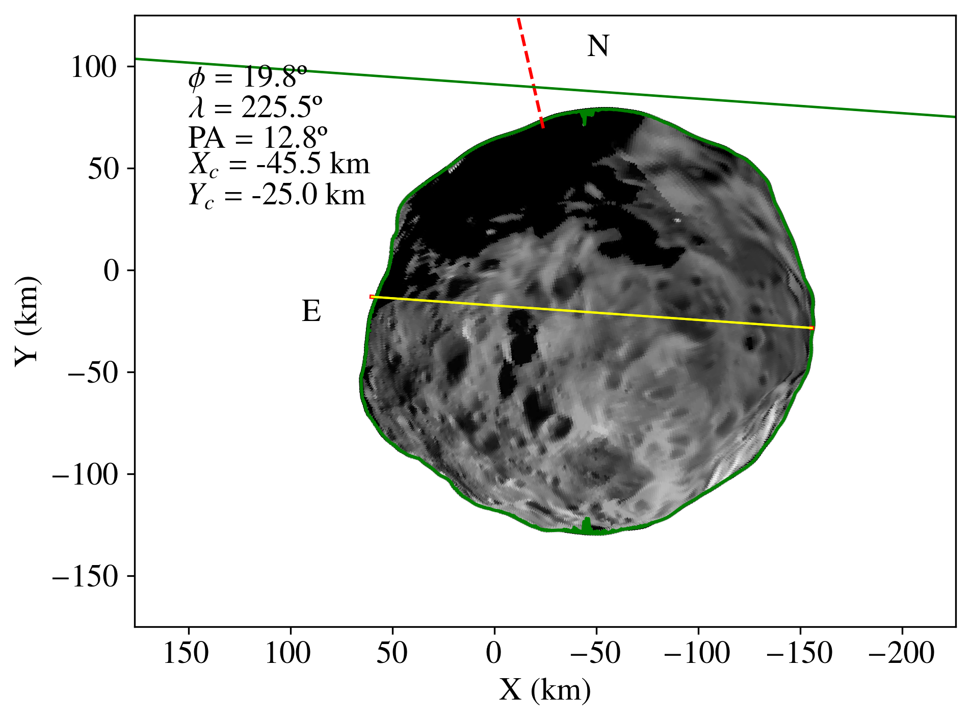
(a) W1 solution

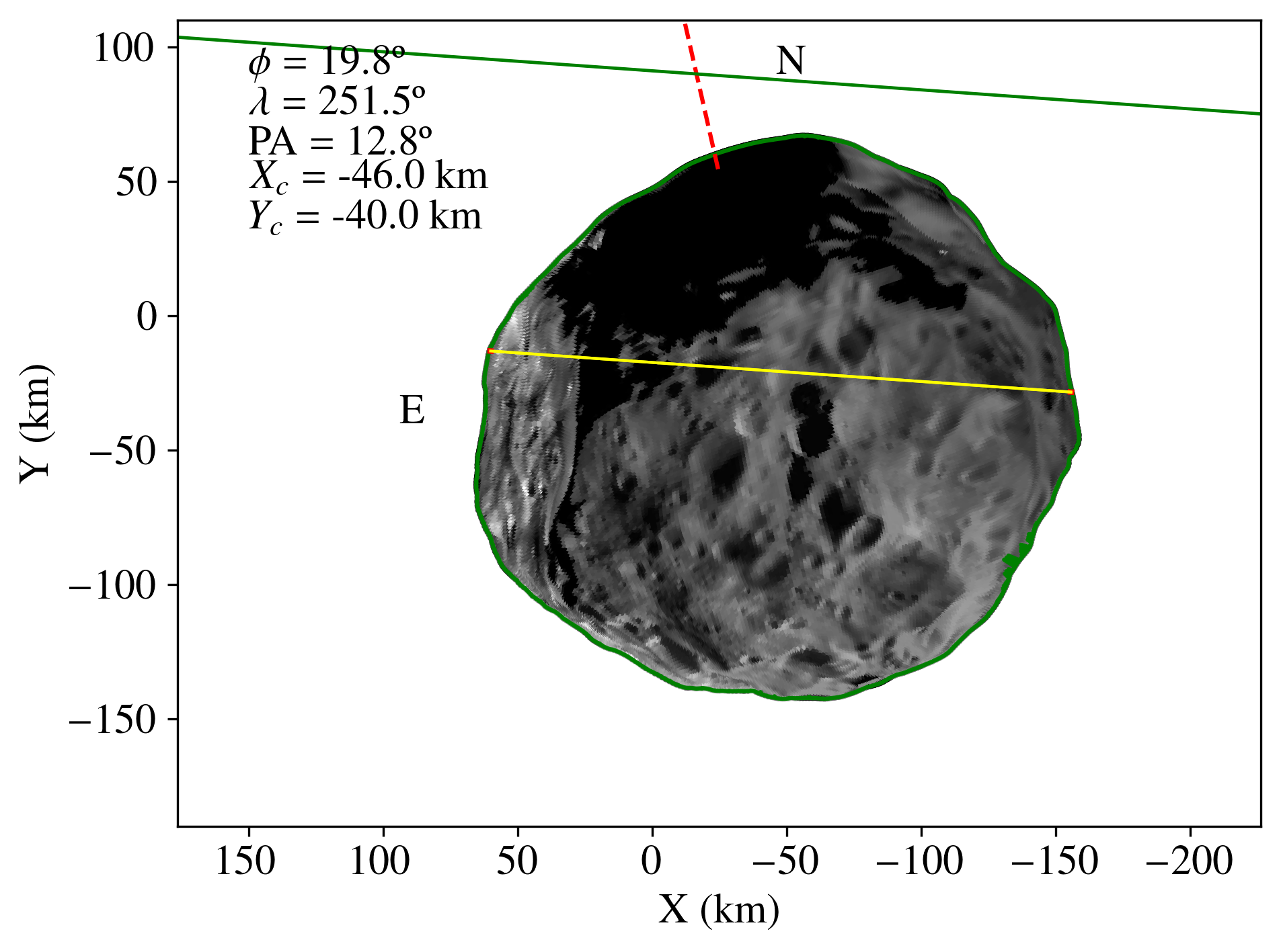
(b) W2 solution

Figure 7: Similar to Figure 3 for the 2018 June 19 occultation. The shapes were obtained using the (a) W1 and (b) W2 rotational period solutions.

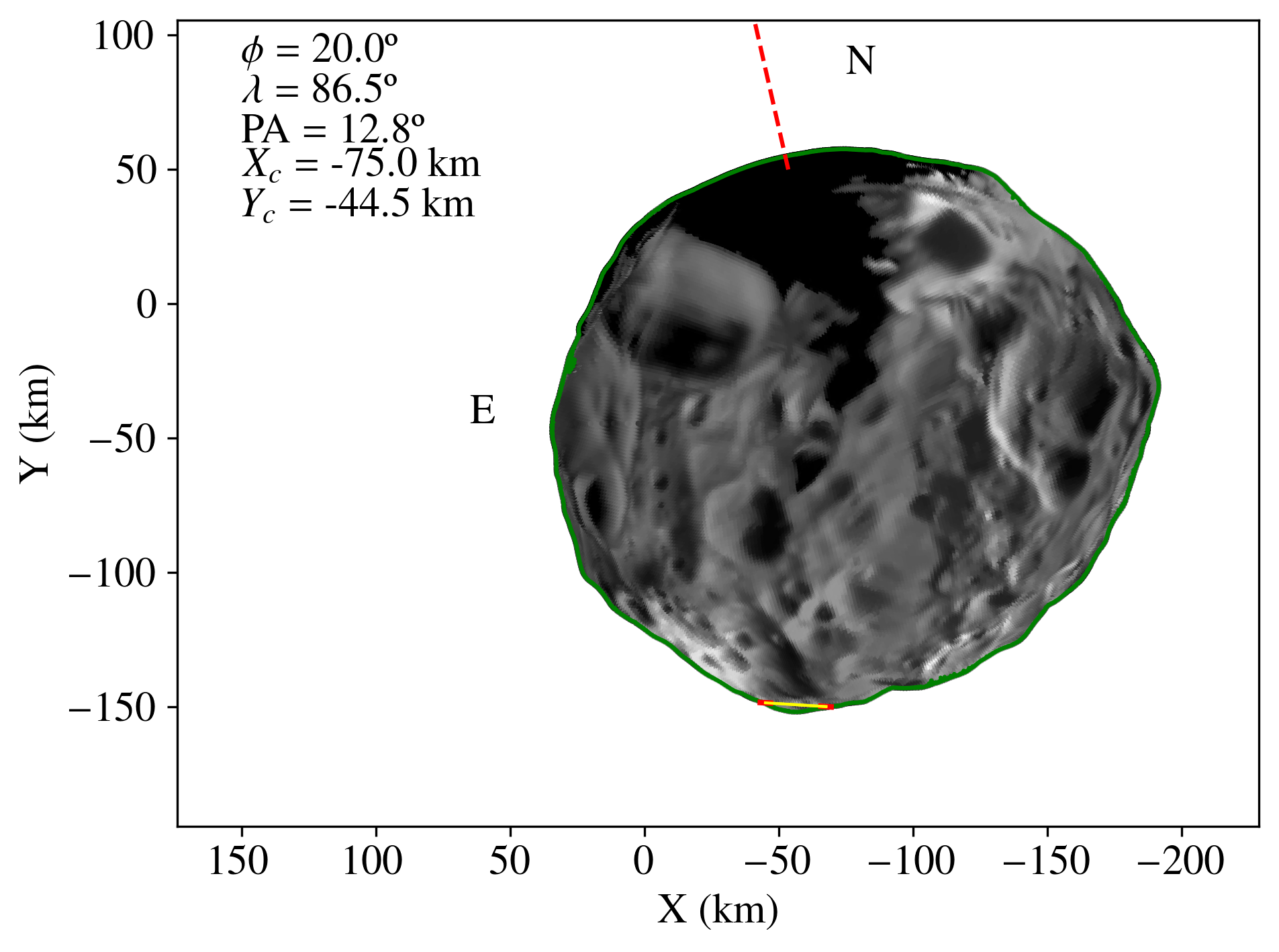
(a) W1 solution

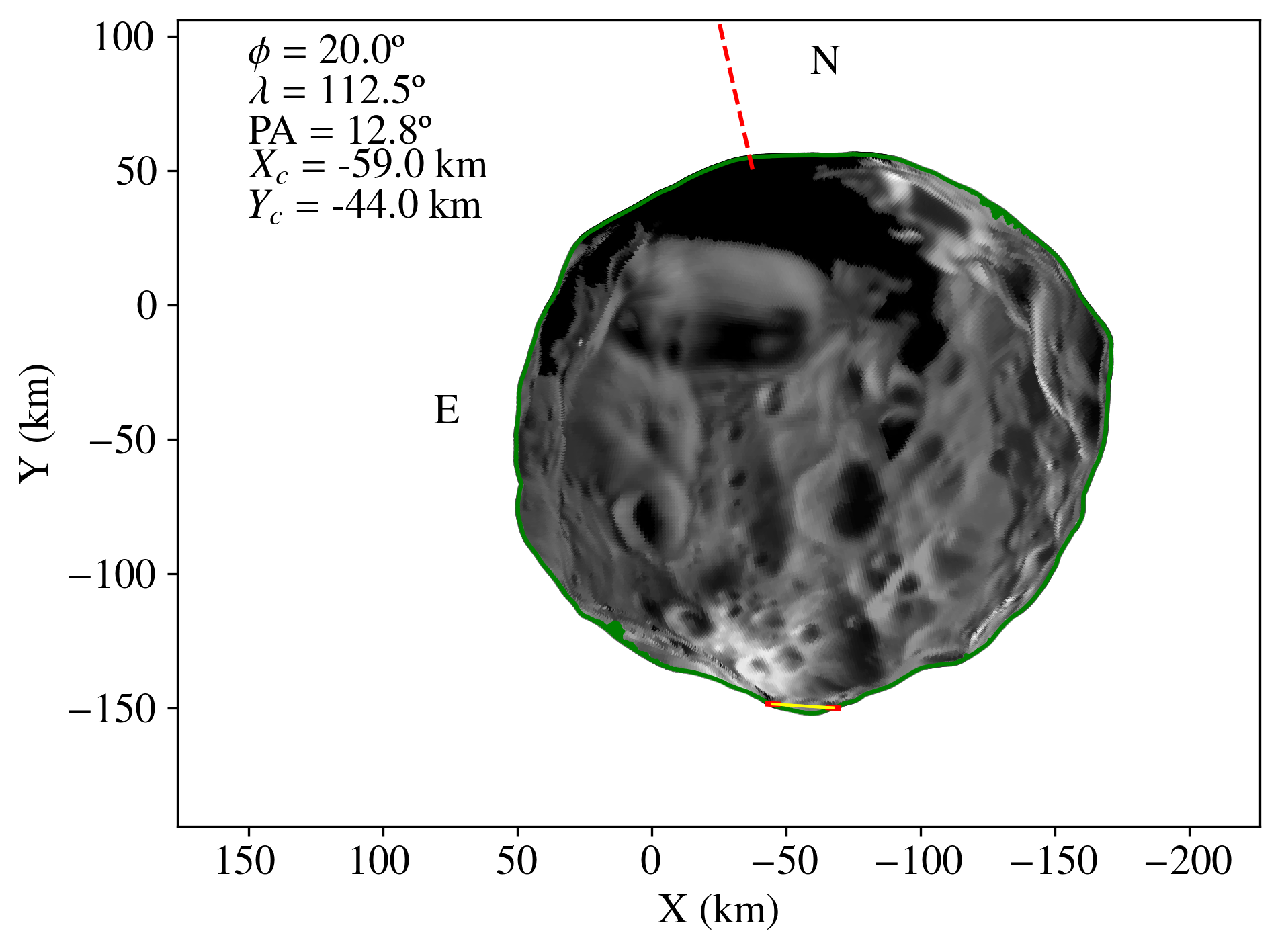
(b) W2 solution

Figure 8: Similar to Figure 7 for the 2018 June 26 occultation.

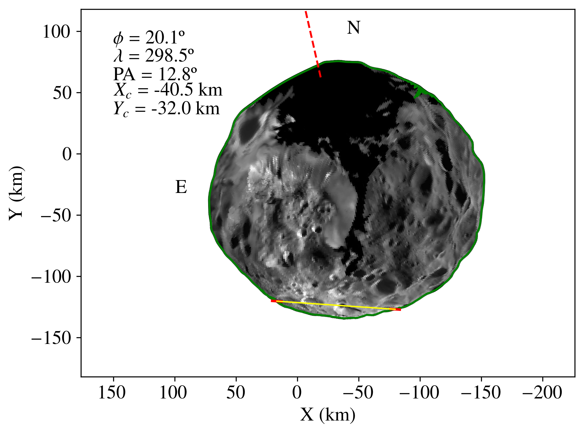
(a) W1 solution

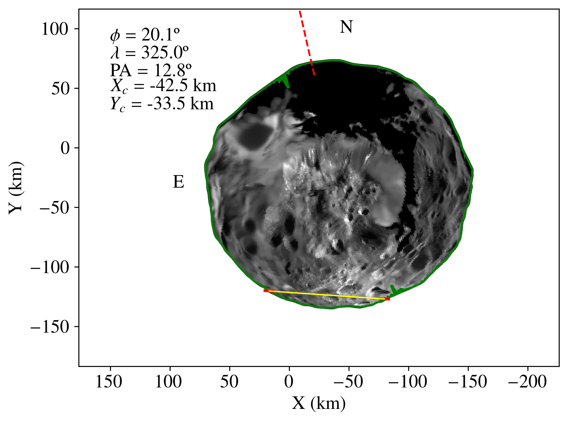
(b) W2 solution

Figure 9: Similar to Figure 7 for the 2018 July 03 occultation.

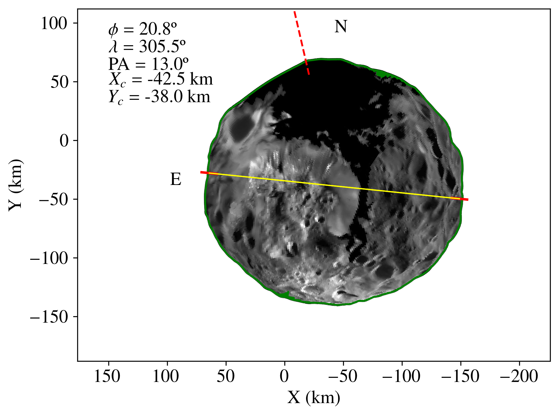
(a) W1 solution

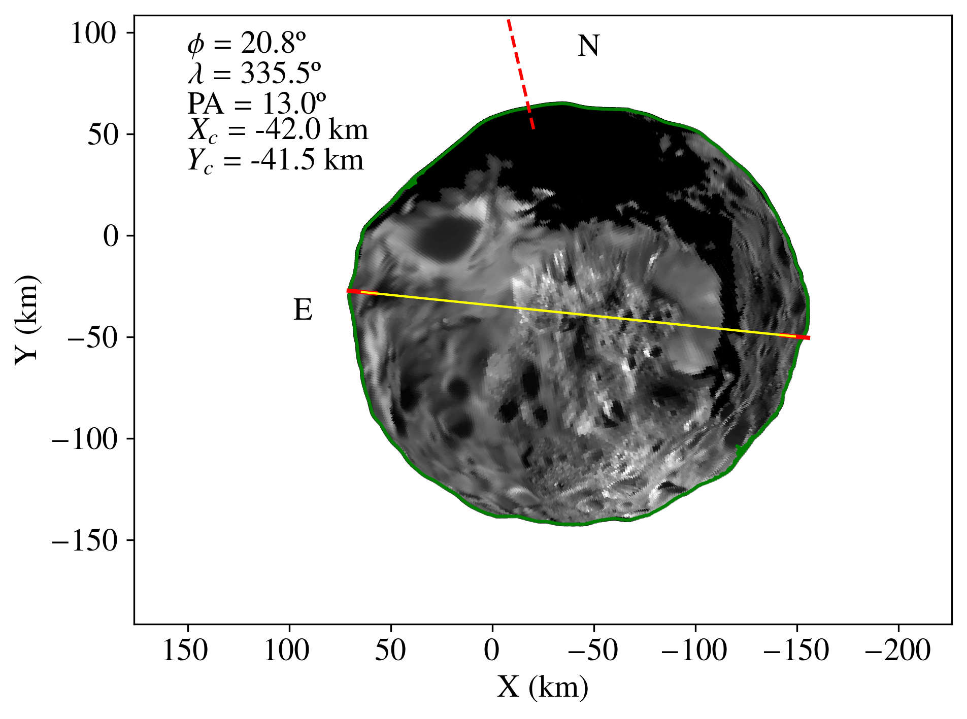
(b) W2 solution

Figure 10: Similar to Figure 7 for the 2018 August 13 occultation. For W2, the mean solution of the north and south solutions combined were considered.

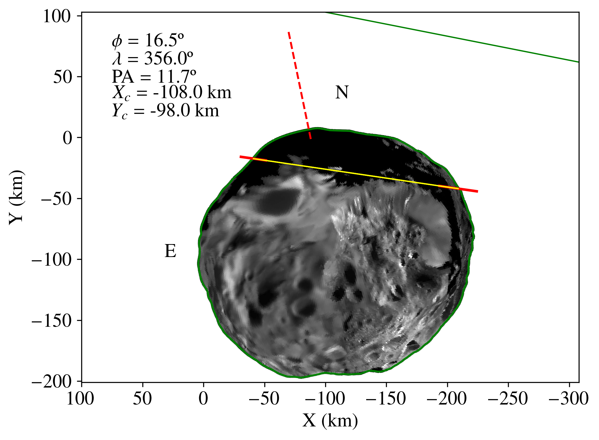
(a) W1 solution

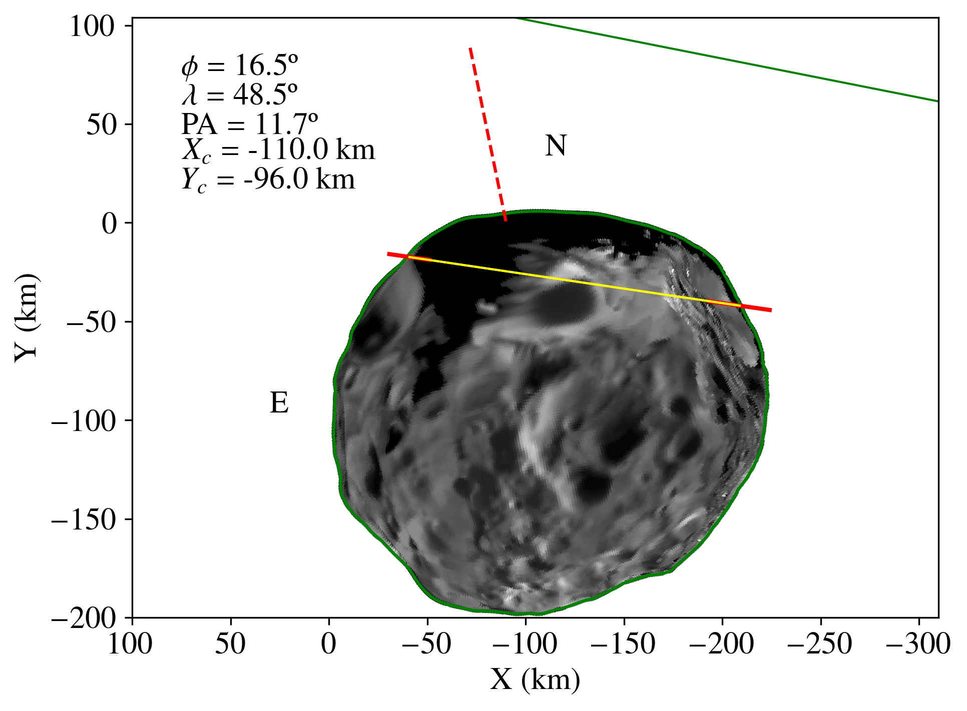
(b) W2 solution

Figure 11: Similar to Figure 7 for the 2019 June 07 occultation.

7 Rotational Light Curve

To check the identified variation in the rotational phase, we obtained the rotational light curve of Phoebe in one night in 2017 from the 1.6m aperture f/10 Perkin-Elmer telescope and two consecutive nights in 2018 from the 0.6m aperture f/13.5 Boller & Chivens telescope. Both telescopes are located at the Observatório do Pico dos Dias (OPD, 45°34′57$\aas@@fstack{\prime\prime}$5 W, 22°32′07$\aas@@fstack{\prime\prime}$8 S, 1864 m) run by Laboratório Nacional de Astrofísica/MCTI, Itajubá/MG, Brazil, IAU code 874. In 2017 July 28, we acquired about 5.5 hours of observations with an I filter, while in 2018 May 23 and 24 we obtained about 5.5 and 7 hours respectively, both without the use of filters. All the observations were made with an IKON camera.

Because Phoebe is crossing a very dense region of stars, a Difference Image Analysis procedure was applied to the observation to remove the background stars. The light curves were then obtained from the subtracted images using praia. Figure 12 shows the light curve (normalised redrelative magnitude) of three nights as a function of the sub-observer longitude obtained from the W2 solution. No fit was done to obtain a new period. The location of the longitude $0\degr$ using the W1 solution and from Archinal et al. (2018) ($W_{A}$) are also shown.

It is important to note that Bauer et al. (2004) assumed the maximum of the curve (maximum brightness) as the $0\degr$ longitude following the longitude system of Colvin et al. (1989). We can see that the maximum in Figure 12 is closer to the $0\degr$ longitude for the W2 solution, while W1 and $W_{A}$ solutions are not.

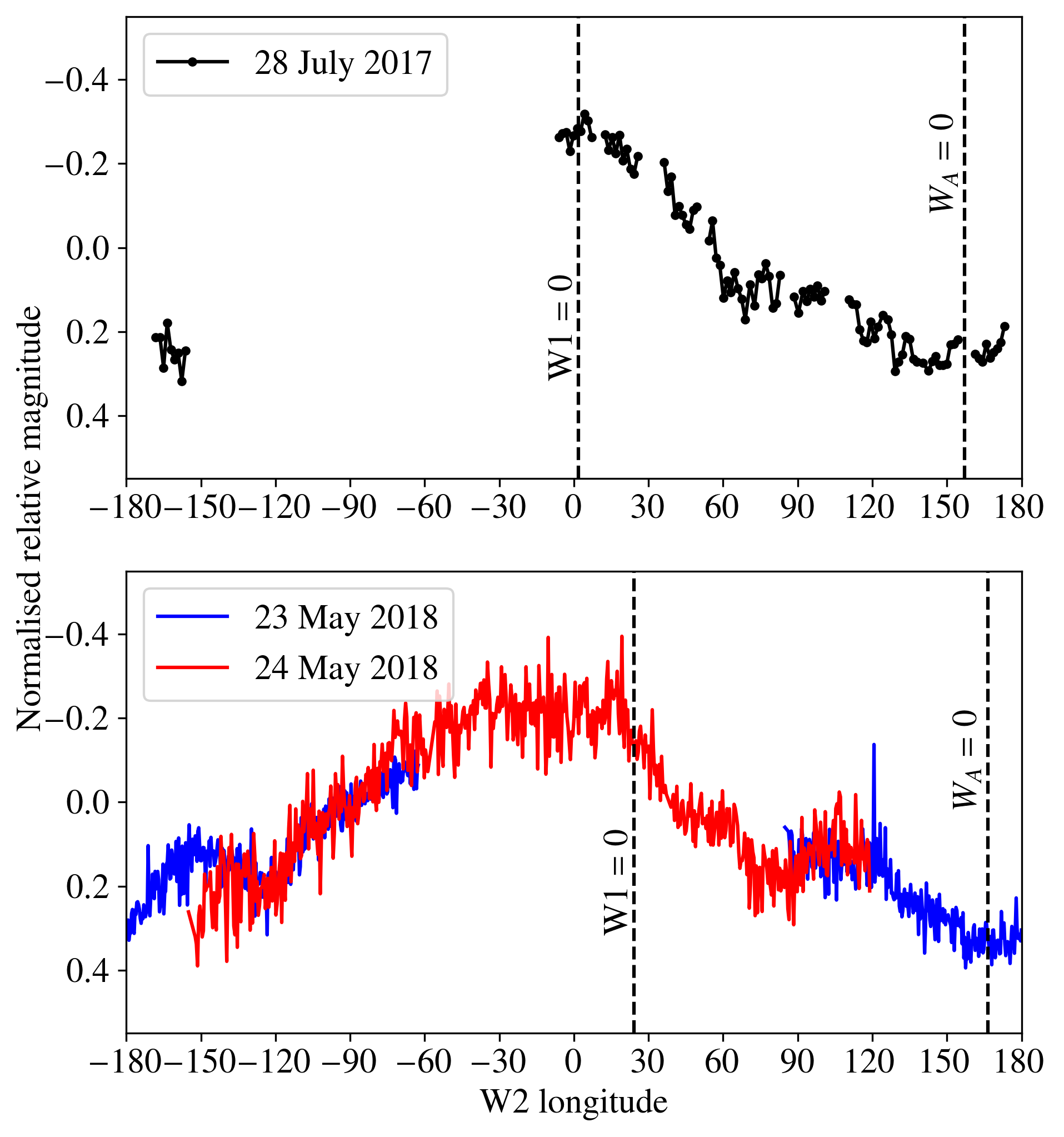
Figure 12: Rotational light curves obtained from one night of observation in 2017 and two nights of observations in 2018 at the OPD. The abscissa is the sub-observer longitude using the W2 solution, as explained in the text. The location of the longitude $0\degr$ using the W1 solution and from Archinal et al ($W_{A}$) are also shown for comparison.

8 Results

8.1 Preferred Rotational Period

As shown in section 5, we managed to identify two possible solutions for the rotation period of Phoebe from the differences in sub-observer longitude determined from the 2017 occultation and the prediction using the rotation model of Archinal et al. (2018). They are S1 = 9.274404 h $\pm$ 0.07 s and S2 = 9.273653 h $\pm$ 0.07 s, respectively related to the W1 and W2 solutions found in section 5.

In section 6, we projected these values for the 2018 and 2019 occultations. The four events of 2018 were observed in an interval of one month, so they are expected to have similar ephemeris offsets. However, using the S1 rotational period solution, the derived position for the centre of Phoebe for the June 26 occultation is fairly inconsistent with the centres from the other occultations. The longitude of the June 19 event would also be very close to a region where the chord is larger than the apparent shape of Phoebe inside the 1-sigma error bar.

Also, as shown in section 7, the maximum of the observed rotational light curve is also near the zero longitude using the S2 solution.

Given these facts and that the S2 solution is also closer to that published by Bauer et al. (2004), S2 (with W2) is our preferred solution. Thus, the redfinal rotational period found for Phoebe is red$9.27365\pm 0.00002$ h.

8.2 Astrometric Results

The fit of the chords to the shape model shows that the prediction of these events was accurate. The possibility to compare the chords with a shape model and the use of Gaia-DR2 stars allows for the determination of very precise astrometric positions for the satellite, with errors in the order of 1 mas.

Table 5 shows the geocentric ICRS coordinates in the Gaia DR2 frame and respective uncertainties for Phoebe from the occultations. The associated sub-observed longitude is also shown in the equation for the preferred W2 (S2) solutions.

Table 5: Geocentric ICRS coordinates in the Gaia DR2 frame, and respective uncertainties for Phoebe from the occultations as described in subsection 8.2.

Date (UTC)	$\alpha$	$\delta$	$\lambda$ (W2)
2017 July 06 16:04:00	$17^{\text{h}}\leavevmode\nobreak\ 31^{\text{m}}\leavevmode\nobreak\ 03\aas@@fstack{s}07802\pm 0.3\text{\leavevmode\nobreak\ mas}$	$-22\degr\leavevmode\nobreak\ 00\arcmin\leavevmode\nobreak\ 57\aas@@fstack{\prime\prime}3585\pm 0.4\text{\leavevmode\nobreak\ mas}$	$126.5\degr\pm 3.5\degr$
2018 June 19 04:38:00	$18^{\text{h}}\leavevmode\nobreak\ 26^{\text{m}}\leavevmode\nobreak\ 16\aas@@fstack{s}38857\pm 0.6\text{\leavevmode\nobreak\ mas}$	$-22\degr\leavevmode\nobreak\ 24\arcmin\leavevmode\nobreak\ 00\aas@@fstack{\prime\prime}5778\pm 0.7\text{\leavevmode\nobreak\ mas}$	$251.5\degr\pm 3.7\degr$
2018 June 26 18:31:00	$18^{\text{h}}\leavevmode\nobreak\ 24^{\text{m}}\leavevmode\nobreak\ 01\aas@@fstack{s}55924\pm 1.1\text{\leavevmode\nobreak\ mas}$	$-22\degr\leavevmode\nobreak\ 26\arcmin\leavevmode\nobreak\ 12\aas@@fstack{\prime\prime}5432\pm 0.4\text{\leavevmode\nobreak\ mas}$	$112.5\degr\pm 3.7\degr$
2018 July 03 13:38:00	$18^{\text{h}}\leavevmode\nobreak\ 22^{\text{m}}\leavevmode\nobreak\ 00\aas@@fstack{s}25759\pm 1.2\text{\leavevmode\nobreak\ mas}$	$-22\degr\leavevmode\nobreak\ 28\arcmin\leavevmode\nobreak\ 10\aas@@fstack{\prime\prime}7045\pm 0.9\text{\leavevmode\nobreak\ mas}$	$325.0\degr\pm 3.7\degr$
2018 Aug 13 12:53:00	$18^{\text{h}}\leavevmode\nobreak\ 12^{\text{m}}\leavevmode\nobreak\ 22\aas@@fstack{s}39941\pm 1.9\text{\leavevmode\nobreak\ mas}$	$-22\degr\leavevmode\nobreak\ 38\arcmin\leavevmode\nobreak\ 44\aas@@fstack{\prime\prime}4513\pm 6.7\text{\leavevmode\nobreak\ mas}$	$335.5\degr\pm 3.7\degr$
2019 June 07 03:54:00	$19^{\text{h}}\leavevmode\nobreak\ 21^{\text{m}}\leavevmode\nobreak\ 18\aas@@fstack{s}59540\pm 2.5\text{\leavevmode\nobreak\ mas}$	$-21\degr\leavevmode\nobreak\ 44\arcmin\leavevmode\nobreak\ 25\aas@@fstack{\prime\prime}6461\pm 2.7\text{\leavevmode\nobreak\ mas}$	$48.5\degr\pm 4.0\degr$

9 Conclusions

The stellar occultation of 2017 July 06 was the first occultation by an irregular satellite ever observed. The observation was possible due to the improved ephemeris developed by Gomes-Júnior et al. (2016) and the fortuitous passage of Phoebe in front of the galactic plane, which allowed to predict more events with bright stars.

Six stellar occultations were observed, one with two positive detections and other five single-chord events. The uncertainties obtained in the ingress and egress instants are of the order of 1 km and reflects the precision of the technique.

Due to the Cassini’s observation of Phoebe, that provided a good knowledge of the shape of the satellite and showed its cratered nature, fitting circular or elliptical shapes to the chords would not provide accurate results. The 3D shape model of Phoebe from Gaskell (2013) allowed a more precise analysis. Comparing the model with the occultation chords, we found that the chords of 2017 July 06 occultation better fit to the model when projecting the model in the sub-observer longitude $\lambda=126.5\pm 3.5\degr$.

We managed to determine redthe rotation period for Phoebe redfrom stellar occultations. For that, we primarily used the differences in sub-observer longitude determined from the two-chord 2017 occultation and from the prediction using the rotation model of Archinal et al. (2018). We eliminated the ambiguity in the solution by using the other single-chord occultations and rotation light curves observed by us and from Bauer et al. (2004). The redfinal rotation period found is p = red$9.27365\pm 0.00002$ h. redAlthough the value is within the error bar of Bauer et al. (2004), our results improve the determination of the rotational period of the satellite by one order of magnitude. The related location of the prime meridian (the half great-circle connecting the body’s north and south pole defined as $\lambda=0\degr$ in the body-centred reference frame) is $W(\degr)=125.56+931.6717d$, following the formalism by Archinal et al. (2018).

We also obtained six geocentric ICRS positions as realised by the GAIA DR2 frame for Phoebe with kilometre accuracy. For comparison, the accuracy of Desmars et al. (2013) ephemeris during the Cassini flyby is in the order of 10 km. The positions obtained here can be helpful to improve the ephemeris and, consequently, the occultation predictions.

The observation of more multi-chord stellar occultations by Phoebe can help to constrain its rotation period better, derive very precise positions and probe uncharted surface features in its northern hemisphere not mapped by Cassini. As predicted by Gomes-Júnior et al. (2016), the density of stellar occultations by Phoebe will decrease after 2019, since Saturn is leaving the apparent galactic plane. Even though the number of favourable events will decrease, we will have better ephemeris and will be able to focus on selected events.

These results with Phoebe give us more expertise and expectation for the campaign of stellar occultations by the Jovian irregular satellites in 2019-2020 when Jupiter, in turn, will be crossing the apparent plane of the Galaxy.

References

- Andrae et al. (2018) Andrae R., Fouesneau M., Creevey O., et al., 2018, Astronomy & Astrophysics, \textcolorred616, \textcolorredA8
- Archinal et al. (2018) Archinal B. A., Acton C. H., A’Hearn M. F., et al., 2018, Celestial Mechanics and Dynamical Astronomy, 130, \textcolorred22
- Assafin et al. (2011) Assafin M., Vieira-Martins R., Camargo J. I. B., et al., 2011, in Tanga P., Thuillot W., eds, Gaia follow-up network for the solar system objects : Gaia FUN-SSO workshop proceedings. pp 85–88
- Bauer et al. (2004) Bauer J. M., Buratti B. J., Simonelli D. P., Owen Jr. W. M., 2004, The Astrophysical Journal, 610, L57–L60
- Benedetti-Rossi et al. (2016) Benedetti-Rossi G., Sicardy B., Buie M. W., et al., 2016, The Astronomical Journal, 152, 156
- Braga-Ribas et al. (2013) Braga-Ribas F., Sicardy B., Ortiz J. L., et al., 2013, ApJ, 773, 26
- Braga-Ribas et al. (2014) Braga-Ribas F., Sicardy B., Ortiz J. L., et al., 2014, Nature, 508, 72–75
- Brown et al. (2018) Brown A. G. A., Vallenari A., Prusti T., et al., 2018, Astronomy & Astrophysics, \textcolorred616, \textcolorredA1
- Clark et al. (2005) Clark R. N., Brown R. H., Jaumann R., et al., 2005, Nature, 435, 66–69
- Colvin et al. (1989) Colvin T., Davies M. E., Rogers P. G., Heller J., 1989, Technical Report STI/Recon. Tech. Rep. N-2934-NASA, Phoebe: A Preliminary Control Network and Rotational Elements. NASA
- Desmars et al. (2013) Desmars J., Li S. N., Tajeddine R., et al., 2013, Astronomy & Astrophysics, 553, A36
- Gaskell (2013) Gaskell R. W., 2013, NASA Planetary Data System, 207
- Gladman et al. (2001) Gladman B., Kavelaars J. J., Holman M., et al., 2001, Nature, 412, 163–166
- Gomes-Júnior et al. (2016) Gomes-Júnior A. R., Assafin M., Beauvalet L., et al., 2016, Monthly Notices of the Royal Astronomical Society, 462, 1351–1358
- Jehin et al. (2011) Jehin E., Gillon M., Queloz D., et al., 2011, The Messenger, 145, 2
- Johnson & Lunine (2005) Johnson T. V., Lunine J. I., 2005, Nature, 435, 69–71
- Michalik et al. (2015) Michalik D., Lindegren L., Hobbs D., 2015, Astronomy & Astrophysics, 574, A115
- Pickering (1899) Pickering E. C., 1899, The Astrophysical Journal, 9, 274
- Porco et al. (2005) Porco C. C., Baker E., Beurle K., et al., 2005, Science, 307, 1237–1242
- Ross (1905) Ross F. E., 1905, Annals of Harvard College Observatory, 53, 101
- Skottfelt et al. (2015) Skottfelt J., Bramich D. M., Hundertmark M., et al., 2015, Astronomy & Astrophysics, 574, A54
- Thomas (2010) Thomas P., 2010, Icarus, 208, 395–401
- Zacharias et al. (2013) Zacharias N., Finch C. T., Girard T. M., Henden A., Bartlett J. L., Monet D. G., Zacharias M. I., 2013, The Astronomical Journal, 145, 44
- van Belle (1999) van Belle G. T., 1999, Publications of the Astronomical Society of the Pacific, 111, 1515–1523