A Jacobi spectral method for computing eigenvalue gaps and their distribution statistics of the fractional Schrödinger operator

Abstract

We propose a spectral method by using the Jacobi functions for computing eigenvalue gaps and their distribution statistics of the fractional Schrödinger operator (FSO). In the problem, in order to get reliable gaps distribution statistics, we have to calculate accurately and efficiently a very large number of eigenvalues, e.g. up to thousands or even millions eigenvalues, of an eigenvalue problem related to the FSO. For simplicity, we start with the eigenvalue problem of FSO in one dimension (1D), reformulate it into a variational formulation and then discretize it by using the Jacobi spectral method. Our numerical results demonstrate that the proposed Jacobi spectral method has several advantages over the existing finite difference method (FDM) and finite element method (FEM) for the problem: (i) the Jacobi spectral method is spectral accurate, while the FDM and FEM are only first order accurate; and more importantly (ii) under a fixed number of degree of freedoms $M$, the Jacobi spectral method can calculate accurately a large number of eigenvalues with the number proportional to $M$, while the FDM and FEM perform badly when a large number of eigenvalues need to be calculated. Thus the proposed Jacobi spectral method is extremely suitable and demanded for the discretization of an eigenvalue problem when a large number of eigenvalues need to be calculated. Then the Jacobi spectral method is applied to study numerically the asymptotics of the nearest neighbour gaps, average gaps, minimum gaps, normalized gaps and their distribution statistics in 1D. Based on our numerical results, several interesting numerical observations (or conjectures) about eigenvalue gaps and their distribution statistics of the FSO in 1D are formulated. Finally, the Jacobi spectral method is extended to the directional fractional Schrödinger operator in high dimensions and extensive numerical results about eigenvalue gaps and their distribution statistics are reported.

url]http://blog.nus.edu.sg/matbwz/

1 Introduction

Consider the eigenvalue problem of the fractional Schrödinger operator (FSO) (or time-independent fractional Schrödinger equation) in one dimension (1D):

Find $\lambda\in\mathbb{R}$ and a nonzero real-valued function $u(x)\neq 0$ such that

$$\begin{split}L_{\rm FSO}\;u(x)&:=\left[(-\partial_{xx})^{\alpha/2}+V(x)\right]u(x)=\lambda\;u(x),\qquad x\in\Omega:=(a,b),\\ u(x)&=0,\qquad x\in\Omega^{c}:=\mathbb{R}\backslash\Omega,\end{split}$$ (1.1)

where $0<\alpha\leq 2$, $V(x)\in L^{2}(\Omega)$ is a given real-valued function and the fractional Laplacian operator (FLO) $(-\partial_{xx})^{\alpha/2}$ is defined via the Fourier transform (see [63, 24, 40] and references therein) as

$$(-\partial_{xx})^{\alpha/2}\;u(x)={\mathcal{F}}^{-1}(|\xi|^{\alpha}(\mathcal{F}u)(\xi))\qquad x,\xi\in\mathbb{R},$$ (1.2)

with ${\mathcal{F}}$ and ${\mathcal{F}}^{-1}$ the Fourier transform and inverse Fourier transform [16, 40, 31], respectively. We remark here that an alternative way to define $(-\partial_{xx})^{\alpha/2}$ is through the principle value integral (see [56, 58, 25, 43, 24] and references therein) as

$$(-\partial_{xx})^{\alpha/2}\;u(x):=C_{1}^{\alpha}\int_{\mathbb{R}}\frac{u(x)-u(y)}{|x-y|^{1+\alpha}}dy,\qquad x\in{\mathbb{R}},$$ (1.3)

where $C_{1}^{\alpha}$ is a constant whose value can be computed explicitly as

$$C_{1}^{\alpha}=\frac{2^{\alpha}\Gamma((1+\alpha)/2)}{\pi^{1/2}|\Gamma(-\alpha/2)|}=\frac{\alpha\Gamma((1+\alpha)/2)}{2^{1-\alpha}\pi^{1/2}\Gamma(1-\alpha/2)}.$$

Another remark here is that the problem (1.1) is equivalent to the problem defined on the whole $x$-axis ${\mathbb{R}}$ by taking the potential $V(x)=+\infty$ for $x\in\Omega^{c}$. When $\alpha=2$, (1.1) collapses to the (classical) time-independent Schrödinger equation (or a standard Sturm-Liouville eigenvalue problem) which has been widely used for determining energy levels and their corresponding stationary states of a quantum particle within an external potential $V(x)$ in quantum physics and chemistry [23] and many other areas [42, 20, 22]. When $\alpha=1$, the FLO $(-\Delta)^{1/2}$ and its variation $(\beta-\Delta)^{1/2}$ with $\beta>0$ a constant have been widely adopted in representing Coulomb interaction and dipole-dipole interaction in two dimensions [5, 7, 17, 34] and modeling relativistic quantum mechanics for boson star [28, 6]. When $0<\alpha<2$, (1.1) is usually referred as the time-independent fractional Schrödinger equation (or fractional eigenvalue problem) which has been widely adopted for computing energy levels and their stationary states in fractional quantum mechanics [43, 7, 17], polariton condensation and quantum fluids of lights [18, 50], while the FSO can be interpreted via the Feynman path integral approach over Brownian-like quantum paths or over the Lévy-like quantum paths, see [58, 43, 35] and references therein.

Without loss of generality, we assume that $V(x)$ is non-negative, i.e. $V(x)\geq 0$ for $x\in\Omega$. Since all eigenvalues of (1.1) are distinct (or all spectrum are discrete and no continuous spectrum), we can rank (or order) all eigenvalues of (1.1) as

$$0<\lambda_{1}^{\alpha}<\lambda_{2}^{\alpha}\leq\ldots\leq\lambda_{n}^{\alpha}\leq\ldots\,,$$ (1.4)

where the times that an eigenvalue $\lambda$ of (1.1) appears in the above sequence (1.4) is the same as its algebraic multiplicity. When $V(x)\equiv 0$ for $x\in\Omega$, all eigenvalues of (1.1) are simple eigenvalues, i.e. their algebraic multiplicities are all equal to $1$, then all $\leq$ in (1.4) can be replaced by $<$. Define the nearest neighbor gaps as [33]

$$\delta_{\rm nn}^{\alpha}(N):=\lambda_{N+1}^{\alpha}-\lambda_{N}^{\alpha},\qquad N=1,2,3,\ldots,$$ (1.5)

where when $N=1$, i.e., $\delta_{\rm nn}^{\alpha}(1)=\lambda_{2}^{\alpha}-\lambda_{1}^{\alpha}:=\delta_{\rm fg}(\alpha)$ (i.e. the difference between the first two smallest eigenvalues) is called as the fundamental gap of the FSO (1.1), which has been studied analytically and/or numerically for $\alpha=2$ [3, 1, 8] and $0<\alpha\leq 2$ [9, 13]; the minimum gaps as [15, 54]

$$\delta_{\rm min}^{\alpha}(N):=\min_{1\leq n\leq N}\ \delta_{\rm nn}^{\alpha}(n)=\min_{1\leq n\leq N}\ \lambda_{n+1}^{\alpha}-\lambda_{n}^{\alpha},\qquad N=1,2,3,\ldots;$$ (1.6)

the average gaps as [33]

$$\delta_{\rm ave}^{\alpha}(N):=\frac{1}{N}\sum_{n=1}^{N}\delta_{\rm nn}^{\alpha}(n)=\frac{1}{N}\sum_{n=1}^{N}\left(\lambda_{n+1}^{\alpha}-\lambda_{n}^{\alpha}\right)=\frac{\lambda_{N+1}^{\alpha}-\lambda_{1}^{\alpha}}{N},\qquad N=1,2,\cdots\;.$$ (1.7)

In addition, if there exist constants $\gamma>0$ and $C>0$ such that

$$\lim_{n\to+\infty}\frac{\lambda_{n}^{\alpha}}{n^{\gamma}}=C>0,$$ (1.8)

then the normalized gaps (or “unfolding” local statistics in the physics literature) are defined as [33, 55]

$$\delta_{\rm norm}^{\alpha}(N):=y_{N+1}^{\alpha}-y_{N}^{\alpha},\qquad N=1,2,\ldots\;,$$ (1.9)

where

$$y_{n}^{\alpha}:=\left(\frac{\lambda_{n}^{\alpha}}{C}\right)^{1/\gamma},\qquad n=1,2,\ldots\;.$$ (1.10)

Then an interesting question is to study their asymptotics, i.e. the behaviour of $\delta_{\rm nn}^{\alpha}(N)$, $\delta_{\rm min}^{\alpha}(N)$, $\delta_{\rm ave}^{\alpha}(N)$ and $\delta_{\rm nrom}^{\alpha}(N)$ when $N\to+\infty$, and another interesting and very challenging question is to study the level spacing distribution $P_{\alpha}(s):=$ limiting distribution of the normalized gaps $\delta_{\rm norm}^{\alpha}(N)$, which is defined as [33, 55]

$$\frac{\#\left\{1\leq n\leq N\ |\ \delta_{\rm norm}^{\alpha}(n)<x\right\}}{N}\stackrel{{\scriptstyle{N\to+\infty}}}{{\to}}\int_{0}^{x}P_{\alpha}(s)ds,\qquad 0\leq x<+\infty,$$ (1.11)

where $\#S$ denotes the number of elements in the set $S$.

When $\alpha=2$ and $V(x)\equiv 0$ in (1.1), it collapses to a standard Sturm-Liouville eigenvalue problem of the Laplacian operator as

$$\begin{split}L_{\rm SO}\;u(x)&:=-\partial_{xx}\,u(x)=-u^{\prime\prime}(x)=\lambda\;u(x),\qquad x\in\Omega=(a,b),\\ u(a)&=u(b)=0.\end{split}$$ (1.12)

The eigenvalues and their corresponding eigenfunctions of (1.12) can be obtained analytically via the sine series as

$$\lambda_{n}^{\alpha=2}=\left(\frac{n\pi}{b-a}\right)^{2},\qquad u_{n}(x)=\sin\left(\frac{n\pi(x-a)}{b-a}\right),\qquad n=1,2,\ldots\ .$$ (1.13)

These results immediately imply that the fundamental gap $\delta_{\rm fg}(\alpha=2)=\frac{3\pi^{2}}{(b-a)^{2}}$ and

$$\begin{split}&\delta_{\rm nn}^{\alpha=2}(N)=\left(\frac{(N+1)\pi}{b-a}\right)^{2}-\left(\frac{N\pi}{b-a}\right)^{2}=\frac{\pi^{2}}{(b-a)^{2}}(2N+1),\\ &\delta_{\rm min}^{\alpha=2}(N)\equiv\delta_{\rm nn}^{\alpha=2}(N=1)=\frac{3\pi^{2}}{(b-a)^{2}},\\ &\delta_{\rm ave}^{\alpha=2}(N)=\frac{1}{N}\left[\left(\frac{(N+1)\pi}{b-a}\right)^{2}-\left(\frac{\pi}{b-a}\right)^{2}\right]=\frac{\pi^{2}}{(b-a)^{2}}(N+2),\\ &\delta_{\rm norm}^{\alpha=2}(N)=y_{N+1}^{\alpha=2}-y_{N}^{\alpha=2}=N+1-N\equiv 1,\end{split}\qquad N=1,2,\ldots\;;$$ (1.14)

where

$$y_{n}^{\alpha=2}=\sqrt{\lambda_{n}^{\alpha=2}/\left(\frac{\pi}{b-a}\right)^{2}}=\sqrt{n^{2}}=n,\qquad n=1,2,\ldots\ .$$

From the last equation in (1.14), one can immediately obtain the level spacing distribution defined in (1.11) for $\alpha=2$ as

$$P_{\alpha=2}(s)=\delta(s-1),\qquad s\geq 0,$$ (1.15)

where $\delta(\cdot)$ is the Dirac delta function.

When $\alpha=2$ and $V(x)\neq 0$ in (1.1), it collapses to a standard Sturm-Liouville eigenvalue problem, which has been extensively studied in the literature. For analytical results, we refer to [38, 42, 32] and references therein. For numerical methods and results, we refer to [12, 4, 59] and references therein.

When $0<\alpha<2$, in general, one cannot find the eigenvalues of the eigenvalue problem (1.1) analytically and/or explicitly. For mathematical theories of the eigenvalue problem (1.1), we refer to [27, 37] and references therein. Some numerical methods have been proposed to solve (1.1) numerically, including an asymptotic method was proposed in [63], a finite element method (FEM) [14] with piecewise linear element was presented in [35] and a finite difference method (FDM) was studied in [26]. The FDM and FEM are usually first order accurate when $0<\alpha<2$ and they can be adapted to compute the first several eigenvalues [35, 26, 14]. However, if we want to calculate accurately and efficiently a very large number of eigenvalues, e.g. up to thousands or even millions eigenvalues, of the eigenvalue problem (1.1) in order to obtain a reliable gaps distribution statistics, the FDM and FEM have severe drawbacks. The main aim of this paper is to propose a spectral method by using the generalized Jacobi functions for computing different eigenvalue gaps and their distribution statistics of the fractional eigenvalue problem related to FSO (1.1). The proposed numerical method has at least two advantages: (i) it is spectral accurate, and more importantly (ii) under a fixed number of degree of freedoms (DOF) $M$, it can calculate accurately a large number of eigenvalues with the number proportional to $M$. Thus this method is a very good candidate for solving our problem, i.e. to compute eigenvalue gaps and their distribution statistics of the fractional eigenvalue problem (1.1).

Based on our extensive numerical results and observations, we speculate the following:

Conjecture (Gaps and their distribution statistics of FSO in (1.1) without potential) Assume $0<\alpha<2$ and $V(x)\equiv 0$ in (1.1), then we have the following asymptotics of its eigenvalues:

$$\lambda_{n}^{\alpha}=\left(\frac{n\pi}{b-a}\right)^{\alpha}-\left(\frac{\pi}{b-a}\right)^{\alpha}\frac{\alpha(2-\alpha)}{4}n^{\alpha-1}+O(n^{\alpha-2})=\lambda_{\rm loc}^{\alpha}(n)\left[1-\frac{\alpha(2-\alpha)}{4n}+O(n^{-2})\right],\ n\geq 1,$$ (1.16)

where $\lambda_{\rm loc}^{\alpha}(n)=\left(\frac{n\pi}{b-a}\right)^{\alpha}$ ($n=1,2,\ldots$) are the eigenvalues of the local fractional Laplacian operator on $\Omega=(a,b)$ with homogeneous Dirichlet boundary condition [8]. From (1.16), we obtain immediately the following approximations of different gaps:

$$\begin{split}&\delta_{\rm nn}^{\alpha}(N)\approx\left(\frac{\pi}{b-a}\right)^{\alpha}\left[\alpha N^{\alpha-1}+\frac{\alpha(\alpha-1)(2+\alpha)}{4}N^{\alpha-2}+O(N^{\alpha-3})\right],\ \ 0<\alpha<2,\\ &\delta_{\rm min}^{\alpha}(N)=\left\{\begin{array}[]{ll}\delta_{\rm nn}^{\alpha}(1)=\lambda_{2}^{\alpha}-\lambda_{1}^{\alpha},&1<\alpha<2,\\ \approx\delta_{\rm nn}^{\alpha}(1)=\lambda_{2}^{\alpha}-\lambda_{1}^{\alpha},&\alpha=1,\\ \delta_{\rm nn}^{\alpha}(N)=\lambda_{N+1}^{\alpha}-\lambda_{N}^{\alpha}\approx\alpha\left(\frac{\pi}{b-a}\right)^{\alpha}N^{\alpha-1},&0<\alpha<1,\\ \end{array}\right.\\ &\delta_{\rm ave}^{\alpha}(N)\approx\left(\frac{\pi}{b-a}\right)^{\alpha}\left\{\begin{array}[]{ll}\vspace{2mm}\left[N^{\alpha-1}+\frac{\alpha(2+\alpha)}{4}N^{\alpha-2}+O(N^{-1})\right],&1<\alpha<2,\\ \vspace{2mm}\left[1+\left(\frac{3}{4}-\frac{b-a}{\pi}\lambda_{1}^{\alpha=1}\right)N^{-1}+O(N^{-2})\right],&\alpha=1,\\ \left[N^{\alpha-1}-\left(\frac{b-a}{\pi}\right)^{\alpha}\lambda_{1}^{\alpha}N^{-1}+O(N^{\alpha-2})\right],&0<\alpha<1,\\ \end{array}\right.\\ &\delta_{\rm norm}^{\alpha}(N)\approx 1+O(N^{-2}),\qquad 0<\alpha<2,\end{split}\qquad N\geq 1.$$ (1.17)

In addition, for the gaps distribution statistics defined in (1.11), we have

$$P_{\alpha}(s)=\delta(s-1),\qquad s\geq 0,\qquad 0<\alpha\leq 2.$$ (1.18)

The paper is organized as follows. In Section 2, we begin with some scaling properties of (1.1) and propose a spectral-Galerkin method by using the generalized Jacobi functions to discretize the fractional eigenvalue problem (1.1). In Section 3, we test the accuracy and resolution capacity (or trust region) with respect to the DOF $M$ of the proposed Jacobi spectral method and compare it with the existing numerical methods such as FDM and FEM. In Section 4, we apply the proposed numerical method to study numerically asymptotics of different eigenvalue gaps and their distribution statistics of (1.1) without potential and formulate several interesting numerical observations (or conjectures). Similar results are reported in Section 5 for (1.1) with potential. Extensions of the numerical method and results to the directional fractional Schrödinger operator in high dimensions are presented in Section 6. Finally, some conclusions are drawn in Section 7.

2 A Jacobi spectral method

In this section, we begin with a scaling argument to the problem (1.1) so as to reduce it on a standard interval $(-1,1)$, then reformulate it into a variational formulation and discretize the problem by using the Jacobi spectral method.

2.1 Scaling property

Introduce

$$x_{0}=\frac{a+b}{2},\qquad L=\frac{b-a}{2},\qquad\tilde{x}=\frac{x-x_{0}}{L},\qquad\tilde{V}(\tilde{x})=L^{\alpha}V(x),\qquad x\in\Omega=(a,b),$$ (2.1)

and consider the re-scaled fractional eigenvalue problem:

Find $\tilde{\lambda}\in\mathbb{R}$ and a real-valued function $\tilde{u}(\tilde{x})\neq 0$ such that

$$\begin{split}\tilde{L}_{\rm FSO}\;\tilde{u}(\tilde{x})&:=\left[(-\partial_{\tilde{x}\tilde{x}})^{\alpha/2}+\tilde{V}(\tilde{x})\right]\tilde{u}(\tilde{x})=\tilde{\lambda}\;\tilde{u}(\tilde{x}),\qquad\tilde{x}\in\tilde{\Omega}:=(-1,1),\\ \tilde{u}(\tilde{x})&=0,\qquad\tilde{x}\in\tilde{\Omega}^{c}:=\mathbb{R}\backslash\tilde{\Omega};\end{split}$$ (2.2)

then we have

Lemma 2.1

Let $\tilde{\lambda}$ be an eigenvalue of (2.2) and $\tilde{u}:=\tilde{u}(\tilde{x})$ be the corresponding eigenfunction, then $\lambda=L^{-\alpha}\tilde{\lambda}$ is an eigenvalue of (1.1) and $u:=u(x)=\tilde{u}(\tilde{x})=\tilde{u}\left(\frac{x-x_{0}}{L}\right)$ is the corresponding eigenfunction. Assume that $0<\tilde{\lambda}_{1}^{\alpha}<\tilde{\lambda}_{2}^{\alpha}\leq\ldots\leq\tilde{\lambda}_{n}^{\alpha}\leq\ldots$ are all eigenvalues of (2.2), then $0<\lambda_{1}^{\alpha}<\lambda_{2}^{\alpha}\leq\ldots\leq\lambda_{n}^{\alpha}\leq\ldots$ (ranked as in (1.4)) with $\lambda_{n}^{\alpha}=L^{-\alpha}\tilde{\lambda}_{n}^{\alpha}$ ($n=1,2,\ldots$) are all eigenvalues of (1.1). In addition, we have the scaling property on the different gaps as

$$\begin{split}&\delta_{\rm nn}^{\alpha}(N)=L^{-\alpha}\tilde{\delta}_{\rm nn}^{\alpha}(N),\qquad\hbox{with}\quad\tilde{\delta}_{\rm nn}^{\alpha}(N):=\tilde{\lambda}_{N+1}^{\alpha}-\tilde{\lambda}_{N}^{\alpha},\\ &\delta_{\rm min}^{\alpha}(N)=L^{-\alpha}\tilde{\delta}_{\rm min}^{\alpha}(N),\qquad\hbox{with}\quad\tilde{\delta}_{\rm min}^{\alpha}(N):=\min_{1\leq n\leq N}\ \tilde{\delta}_{\rm nn}^{\alpha}(n),\\ &\delta_{\rm ave}^{\alpha}(N)=L^{-\alpha}\tilde{\delta}_{\rm ave}^{\alpha}(N),\qquad\hbox{with}\quad\tilde{\delta}_{\rm ave}^{\alpha}(N):=\frac{1}{N}\sum_{n=1}^{N}\tilde{\delta}_{\rm nn}^{\alpha}(n),\\ &\delta_{\rm norm}^{\alpha}(N)=\tilde{\delta}_{\rm norm}^{\alpha}(N),\qquad\hbox{with}\quad\tilde{\delta}_{\rm norm}^{\alpha}(N):=\tilde{y}_{N+1}^{\alpha}-\tilde{y}_{N}^{\alpha},\quad\tilde{y}_{N}^{\alpha}=\left(\frac{\tilde{\lambda}_{N}^{\alpha}}{L^{\alpha}C}\right)^{1/\gamma},\end{split}\quad N=1,2,\ldots\;;$$ (2.3)

which immediately imply that the level spacing distribution $P_{\alpha}(s)$ of (1.1) does not change under the rescaling (2.1), i.e. the problems (1.1) and (2.2) have the same level spacing distribution.

Proof: From (1.3) and noticing (2.1), a direct computation implies the scaling property of the fractional Laplacian operator

$$(-\partial_{xx})^{\alpha/2}\,u(x) = C_{1}^{\alpha}\int_{\mathbb{R}}\frac{u(x)-u(y)}{|x-y|^{1+\alpha}}\,dy=C_{1}^{\alpha}\int_{\mathbb{R}}\frac{u(x_{0}+L\tilde{x})-u(x_{0}+L\tilde{y})}{|x_{0}+L\tilde{x}-x_{0}-L\tilde{y}|^{1+\alpha}}\,L\,{d\tilde{y}}$$ (2.4)

$$= L^{-\alpha}C_{1}^{\alpha}\int_{\mathbb{R}}\frac{\tilde{u}(\tilde{x})-\tilde{u}(\tilde{y})}{|\tilde{x}-\tilde{y}|^{1+\alpha}}\,d\tilde{y}=L^{-\alpha}\,(-\partial_{\tilde{x}\tilde{x}})^{\alpha/2}\,\tilde{u}(\tilde{x}),\quad x\in\Omega,\quad\tilde{x}\in\tilde{\Omega}.$$

Noticing

$$u(x)=0,\quad x\in\Omega^{c}\qquad\Longleftrightarrow\qquad\tilde{u}(\tilde{x})=0,\quad\tilde{x}\in\tilde{\Omega}^{c}.$$ (2.5)

Substituting (2.4) into (2.2), noting (1.1), we get

$$\tilde{\lambda}\,u(x) = \tilde{\lambda}\,\tilde{u}(\tilde{x})=\left[(-\partial_{\tilde{x}\tilde{x}})^{\frac{\alpha}{2}}+\tilde{V}(\tilde{x})\right]\tilde{u}(\tilde{x})=\left[L^{\alpha}\,(-\partial_{xx})^{\frac{\alpha}{2}}+\tilde{V}\left(\frac{x-x_{0}}{L}\right)\right]u(x)$$ (2.6)

$$= L^{\alpha}\left[(-\partial_{xx})^{\frac{\alpha}{2}}+L^{-\alpha}\tilde{V}\left(\frac{x-x_{0}}{L}\right)\right]u(x)=L^{\alpha}\left[(-\partial_{xx})^{\frac{\alpha}{2}}+V(x)\right]u(x),\ x\in\Omega,\ \tilde{x}\in\tilde{\Omega},\quad$$

which immediately implies that $u(x)$ is an eigenfunction of the operator $(-\partial_{xx})^{\frac{\alpha}{2}}+V(x)$ with the eigenvalue $\lambda=L^{-\alpha}\tilde{\lambda}$.

From the assumption (1.4) with $\Omega=(-1,1)$ that $0<\tilde{\lambda}_{1}^{\alpha}<\tilde{\lambda}_{2}^{\alpha}\leq\ldots\leq\tilde{\lambda}_{n}^{\alpha}\leq\ldots$ are all eigenvalues of (2.2), we get immediately that $0<\lambda_{1}^{\alpha}<\lambda_{2}^{\alpha}\leq\ldots\leq\lambda_{n}^{\alpha}\leq\ldots$ with $\lambda_{n}^{\alpha}=L^{-\alpha}\tilde{\lambda}_{n}^{\alpha}$ ($n=1,2,\ldots$) are all eigenvalues of the eigenvalue problem (1.1). Then the scaling property on the different gaps (2.3) can be obtained straightforward by using $\tilde{\lambda}_{n}^{\alpha}=L^{\alpha}\lambda_{n}^{\alpha}$ ($n=1,2,\ldots$). $\Box$

2.2 A variational formulation

Following those in the literature [39, 30], we introduce the fractional functional space $H^{\frac{\alpha}{2}}(\mathbb{R})$ through the Fourier transform

$$H^{\frac{\alpha}{2}}(\mathbb{R})=\left\{v\in\mathcal{D}^{\prime}(\mathbb{R})\ |\ \|v\|_{\frac{\alpha}{2},\mathbb{R}}<\infty\right\},$$ (2.7)

where the norms are defined as

$$|v|_{\frac{\alpha}{2},\mathbb{R}}=\left(\int_{\mathbb{R}}\left|\xi|^{\alpha}\right|\;\left|(\mathcal{F}v)(\xi)\right|^{2}\,d\xi\right)^{\frac{1}{2}},\qquad\|v\|_{\frac{\alpha}{2},\mathbb{R}}=\left(\int_{\mathbb{R}}(1+|\xi|^{2})^{\frac{\alpha}{2}}\left|(\mathcal{F}v)(\xi)\right|^{2}d\xi\right)^{\frac{1}{2}};$$ (2.8)

and then the fractional functional space $H^{\frac{\alpha}{2}}(\Omega)$ can be obtained from $H^{\frac{\alpha}{2}}(\mathbb{R})$ by extension [39, 30]

$$H^{\frac{\alpha}{2}}(\Omega)=\left\{v:\;\Omega\to\mathbb{R}\ |\ \hat{v}=E_{\Omega}v\in H^{\frac{\alpha}{2}}(\mathbb{R})\right\},$$ (2.9)

where the norms are defined as

$$|v|_{\frac{\alpha}{2}}:=|v|_{\frac{\alpha}{2},\Omega}=|E_{\Omega}v|_{\frac{\alpha}{2},\mathbb{R}},\qquad\|v\|_{\frac{\alpha}{2}}:=\|v\|_{\frac{\alpha}{2},\Omega}=\|E_{\Omega}v\|_{\frac{\alpha}{2},\mathbb{R}},\qquad\forall v\in H^{\frac{\alpha}{2}}(\Omega),$$ (2.10)

with $\hat{v}=E_{\Omega}v:\mathbb{R}\to\mathbb{R}$ (extension of $v$ from $\Omega$ to $\mathbb{R}$) defined as

$$\hat{v}(x)=(E_{\Omega}v)(x)=\left\{\begin{array}[]{ll}v(x),&x\in\Omega,\\ 0,&x\in\mathbb{R}\backslash\Omega.\\ \end{array}\right.$$ (2.11)

For any $v\in H^{\frac{\alpha}{2}}(\Omega)$, multiplying $v$ to (1.1) and integrating over $\Omega$ and using integration by parts, we obtain the variational (or weak) formulation of the fractional eigenvalue problem (1.1) as:

find $\lambda\in\mathbb{R}$ and $0\neq u\in H^{\frac{\alpha}{2}}(\Omega)$, such that

$$a(u,v)=\lambda\;b(u,v),\qquad\forall v\in H^{\frac{\alpha}{2}}(\Omega),$$ (2.12)

where the bilinear forms $a(\cdot,\cdot)$ and $b(\cdot,\cdot)$ are given as

$$\begin{split}&a(u,v)=\int_{\Omega}\left[(-\partial_{xx})^{\frac{\alpha}{2}}u+V(x)u\right]vdx=\int_{\Omega}\left[(-\partial_{xx})^{\frac{\alpha}{4}}u\;(-\partial_{xx})^{\frac{\alpha}{4}}v+V(x)uv\right]dx,\\ &b(u,v)=\int_{\Omega}u(x)v(x)dx,\qquad\forall u,v\in H^{\frac{\alpha}{2}}(\Omega).\end{split}$$ (2.13)

2.3 A spectral discretization by using the Jacobi functions

Since we are mainly interested in gaps and their distribution statistics, from the results in Lemma 2.1, without loss of generality, from now on, we always assume that $\Omega=(-1,1)$, i.e. $a=-1$ and $b=1$ in (1.1).

Let $\{P_{n}^{\frac{\alpha}{2},\frac{\alpha}{2}}(x)\}_{n=0}^{\infty}$ denote the classical Jacobi polynomials (or Gegenbauer polynomials) which are orthogonal with respect to the weight function $\omega^{\frac{\alpha}{2},\frac{\alpha}{2}}(x)=(1-x^{2})^{\frac{\alpha}{2}}$ over the interval $(-1,1)$, i.e.

$$\int_{-1}^{1}P_{n}^{\frac{\alpha}{2},\frac{\alpha}{2}}(x)\,P_{m}^{\frac{\alpha}{2},\frac{\alpha}{2}}(x)\,\omega^{\frac{\alpha}{2},\frac{\alpha}{2}}(x)dx=C_{n}\delta_{nm},\qquad n,m=0,1,2,\ldots,$$ (2.14)

where $\delta_{nm}$ is the kronecker delta and

$$C_{n}=\frac{2^{\alpha+1}}{2n+\alpha+1}\frac{\Gamma(n+\alpha/2+1)^{2}}{\Gamma(n+\alpha+1)n!}\qquad n=0,1,2\ldots\;.$$ (2.15)

Define the generalized Jacobi functions

$$\mathcal{J}_{n}^{-\frac{\alpha}{2},-\frac{\alpha}{2}}(x)=(1-x^{2})^{\frac{\alpha}{2}}P_{n}^{\frac{\alpha}{2},\frac{\alpha}{2}}(x)=\omega^{\frac{\alpha}{2},\frac{\alpha}{2}}(x)\,P_{n}^{\frac{\alpha}{2},\frac{\alpha}{2}}(x),\quad-1\leq x\leq 1,\qquad n=0,1,2,\ldots,$$ (2.16)

then by Theorem 2 in Ref. [44], we have

$$(-\partial_{xx})^{\frac{\alpha}{2}}\mathcal{J}_{n}^{-\frac{\alpha}{2},-\frac{\alpha}{2}}(x)=\frac{\Gamma(n+\alpha+1)}{n!}P^{\frac{\alpha}{2},\frac{\alpha}{2}}_{n}(x),\quad-1<x<1,\qquad n=0,1,2,\ldots\;.$$ (2.17)

Combining (2.16) and (2.17), we obtain

$$\begin{split}&\int_{-1}^{1}(-\partial_{xx})^{\frac{\alpha}{2}}\mathcal{J}_{n}^{-\frac{\alpha}{2},-\frac{\alpha}{2}}(x)\;\mathcal{J}_{m}^{-\frac{\alpha}{2},-\frac{\alpha}{2}}(x)\;dx=\int_{-1}^{1}\mathcal{J}_{n}^{-\frac{\alpha}{2},-\frac{\alpha}{2}}(x)\;(-\partial_{xx})^{\frac{\alpha}{2}}\mathcal{J}_{m}^{-\frac{\alpha}{2},-\frac{\alpha}{2}}(x)\;dx\\ &\ =\int_{-1}^{1}(-\partial_{xx})^{\frac{\alpha}{4}}\mathcal{J}_{n}^{-\frac{\alpha}{2},-\frac{\alpha}{2}}(x)\;(-\partial_{xx})^{\frac{\alpha}{4}}\mathcal{J}_{m}^{-\frac{\alpha}{2},-\frac{\alpha}{2}}(x)\;dx=\int_{-1}^{1}\frac{\Gamma(n+\alpha+1)}{n!}P^{\frac{\alpha}{2},\frac{\alpha}{2}}_{n}(x)\;\mathcal{J}_{m}^{-\frac{\alpha}{2},-\frac{\alpha}{2}}(x)\;dx\\ &\ =\frac{\Gamma(n+\alpha+1)}{n!}\int_{-1}^{1}P^{\frac{\alpha}{2},\frac{\alpha}{2}}_{n}(x)\;P_{m}^{\frac{\alpha}{2},\frac{\alpha}{2}}(x)\,\omega^{\frac{\alpha}{2},\frac{\alpha}{2}}(x)\;dx\\ &\ =\frac{2^{\alpha+1}\Gamma(n+\alpha/2+1)^{2}}{(n!)^{2}(2n+\alpha+1)}\delta_{nm},\quad n,m=0,1,2\ldots\;.\end{split}$$ (2.18)

Introduce

$$\phi_{n}(x):=\frac{\sqrt{2n+\alpha+1}n!}{2^{\alpha/2+1/2}\Gamma(n+\alpha/2+1)}\mathcal{J}_{n}^{-\frac{\alpha}{2},-\frac{\alpha}{2}}(x),\quad-1\leq x\leq 1,\qquad n=0,1,2,\ldots\;.$$ (2.19)

Let $M>0$ be a positive integer and define the finite dimensional space (which is an approximate subspace of $H^{\frac{\alpha}{2}}(\Omega)$) as

$$\mathbb{W}_{M}:=\mbox{span}\left\{\phi_{m}(x),\ 0\leq m\leq M-1\right\},$$ (2.20)

then a Jacobi spectral method (JSM) for (2.12) is given as:

Find $\lambda_{M}\in\mathbb{R}$ and $0\neq u_{M}\in\mathbb{W}_{M}$ such that

$$a(u_{M},v_{M})=\lambda_{M}\,b(u_{M},v_{M}),\qquad\forall v_{M}\in\mathbb{W}_{M}.$$ (2.21)

In order to cast the eigenvalue problem (2.21) into matrix form, we express $u_{M}\in\mathbb{W}_{M}$ as a combination of the basis functions as

$$u_{M}(x)=\sum^{M-1}_{m=0}\hat{u}_{m}\,\phi_{m}(x),\qquad-1\leq x\leq 1.$$ (2.22)

Plugging (2.22) into (2.21) and noticing (2.18), after some detailed computation, we obtain the following standard matrix eigenvalue problem:

$$\left({\bf I}_{M}+\mathbf{V}\right)\hat{U}=\lambda_{M}\;\mathbf{B}\;\hat{U},$$ (2.23)

where $\hat{U}=(\hat{u}_{0},\hat{u}_{1},\cdots,\hat{u}_{M-1})^{T}\in\mathbb{R}^{M}$ is the eigenvector, ${\bf I}_{M}$ is the $M\times M$ identity matrix, and $\mathbf{V}=(v_{nm})_{0\leq n,m\leq M-1}\in\mathbb{R}^{M\times M}$ and $\mathbf{B}=(b_{nm})_{0\leq n,m\leq M-1}\in\mathbb{R}^{M\times M}$ are given as

$$\begin{split}&v_{nm}=\int_{-1}^{1}V(x)\phi_{n}(x)\phi_{m}(x)dx,\\ &b_{nm}=\int_{-1}^{1}\phi_{n}(x)\phi_{m}(x)dx,\end{split}\qquad n,m=0,1,\ldots,M-1.$$ (2.24)

Plugging (2.19) into the second equation in (2.24), after a detailed computation, we get

$$b_{nm}=\left\{\begin{array}[]{ll}\displaystyle\frac{(-1)^{\frac{n-m}{2}}\sqrt{\pi(2n+\alpha+1)(2m+\alpha+1)}\Gamma(\alpha+1)(n+m)!}{2^{\alpha+n+m+1}\Gamma(\alpha+\frac{n+m}{2}+\frac{3}{2})\Gamma(\frac{\alpha}{2}+\frac{n-1}{2}+1)\Gamma(\frac{\alpha}{2}+\frac{m-1}{2}+1)(\frac{n+m}{2})!},&\hbox{$n+m$~{}even,}\\ 0,&\hbox{$n+m$~{}odd.}\end{array}\right.$$ (2.25)

If $V(x)\equiv 0$, then $\mathbf{V}={\bf 0}$. Of course, if $V(x)\neq 0$, then the integrals in the first equation in (2.24) can be computed numerically via numerical quadratures with spectral accuracy [52, 11]. Finally the matrix eigenvalue problem (2.23) can be solved numerically by the standard eigenvalue solvers such as QR-method [46].

We remark here that different numerical methods have been proposed in the literature for discretizing the fractional Laplacian operator $(-\partial_{xx})^{\alpha/2}$ via the formulation (1.3) or (1.2) or their equivalent forms for numerical simulation of fractional partial differential equations, see [41, 62, 2, 44, 49, 53, 21] and references therein. In fact, a method to discretize the fractional Laplacian operator $(-\partial_{xx})^{\alpha/2}$ can directly generate a method to solve the fractional eigenvalue problem (1.1). For example, a finite element method (FEM) with piecewise linear elements was proposed and analyzed in [35, 14] for computing the eigenvalues of (1.1). Similarly, if we adopt the standard finite difference method to discretize the fractional Laplacian operator $(-\partial_{xx})^{\alpha/2}$ [19, 41] in (1.1), we can obtain a finite difference method (FDM) for computing the eigenvalues of (1.1). The details are omitted here for brevity.

3 Accuracy and comparison with existing methods

In this section, we test the accuracy and resolution capacity of the Jacobi specral method (JSM) presented in the previous section and compare it with the fractional centered finite difference method (FDM) proposed in [62, 19] and the finite element method (FEM) with piecewise linear element proposed in [35] for the eigenvalue problem (1.1) with $\Omega=(-1,1)$. The ‘exact’ eigenvalues $\lambda_{n}^{\alpha}$ ($n=1,2,\ldots$) are obtained numerically by using the JSM (2.21) under a very large DOF $M=M_{0}$, e.g. $M_{0}=12800$. Let $\lambda_{n,M}^{\alpha}$ be the numerical approximation of $\lambda_{n}^{\alpha}$ ($n=1,2,\ldots,M$) obtained by a numerical method with the DOF chosen as $M$. Define the absolute and relative errors of $\lambda_{n}^{\alpha}$ as

$$e_{n}^{\alpha}:=\left|\lambda_{n}^{\alpha}-\lambda_{n,M}^{\alpha}\right|,\qquad e_{n,r}^{\alpha}:=\frac{\left|\lambda_{n}^{\alpha}-\lambda_{n,M}^{\alpha}\right|}{\lambda_{n}^{\alpha}},\qquad n=1,2,\ldots,$$ (3.1)

respectively.

3.1 Accuracy test

We first test the convergence rates of different numerical methods for the eigenvalue problem (1.1) including the JSM (2.21), FEM [35, 14] and FDM [62, 19, 26]. Table 1 displays the absolute errors of computing the first eigenvalue of (1.1) with $V(x)\equiv 0$ and different $\alpha$ by using our JSM (2.21), FEM [35] and FDM [62, 19]; and Table 2 lists the absolute errors of computing the first, second, fifth and tenth eigenvalues of (1.1) with $\alpha=0.5$ and $V(x)\equiv 0$ by using those methods. For comparison with existing results, Table 3 lists the first three eigenvalues of (1.1) with $V(x)\equiv 0$ and different $\alpha$ obtained by using our JSM (2.21) under the DOF $M=160$ and the asymptotic method in [63] under the DOF $M=5000$. Figure 1 shows convergence rates of our JSM (2.21) for computing the first, second, fifth and tenth eigenvalues of (1.1) with $V(x)\equiv 0$ and different $\alpha$; and Figure 2 lists similar results of (1.1) with $V(x)=\frac{x^{2}}{2}$ and different $\alpha$.

		$M=2$	$M=4$	$M=8$	$M=16$	$M=32$	$M=64$	$M=128$	$M=256$
	JSM	3.63E-5	8.47E-9	1.36E-12	1.36E-12	1.39E-12	1.40E-12	1.17E-12	3.62E-12
$\alpha=2.0$	FEM	5.32E-1	1.29E-1	3.18E-2	7.92E-3	1.97E-3	4.87E-4	1.16E-4	2.32E-5
	FDM	4.67E-1	1.24E-1	3.15E-2	7.90E-3	1.97E-3	4.87E-4	1.16E-4	2.32E-5
	JSM	3.18E-5	1.68E-8	1.78E-11	2.49E-12	2.55E-12	2.24E-12	3.08E-12	2.12E-12
$\alpha=1.95$	FEM	4.96E-1	1.16E-2	2.79E-2	6.86E-3	1.72E-3	4.49E-4	1.24E-4	3.78E-5
	FDM	2.31E-1	2.86E-2	5.16E-3	5.41E-4	2.75E-5	7.56E-6	3.76E-6	1.18E-6
	JSM	2.31E-6	7.17E-7	1.57E-8	1.72E-10	2.16E-12	1.02E-12	6.64E-13	1.41E-12
$\alpha=1.5$	FEM	2.72E-1	6.86E-2	2.55E-2	1.18E-2	5.86E-3	2.96E-3	1.49E-3	7.53E-4
	FDM	9.15E-2	6.78E-2	5.41E-2	3.21E-2	1.73E-2	9.01E-3	4.59E-3	2.31E-3
	JSM	2.16E-5	6.32E-6	3.56E-7	1.15E-8	2.65E-10	4.67E-12	5.94E-13	5.53E-13
$\alpha=1.0$	FEM	1.66E-1	5.97E-2	2.29E-2	1.51E-2	7.83E-3	4.01E-3	2.03E-3	1.01E-3
	FDM	1.15E-1	1.00E-1	6.03E-2	3.28E-2	1.71E-2	8.77E-3	4.44E-3	2.24E-3
	JSM	1.22E-4	3.14E-5	3.95E-6	3.65E-7	2.80E-8	1.94E-9	1.26E-10	7.10E-12
$\alpha=0.5$	FEM	8.74E-2	3.93E-2	2.03E-2	1.06E-2	5.54E-3	2.84E-3	1.45E-3	7.35E-4
	FDM	1.08E-1	7.00E-2	3.87E-2	2.04E-2	1.05E-2	5.40E-3	2.74E-3	1.38E-3
	JSM	1.29E-4	4.01E-5	8.58E-6	1.57E-6	2.68E-7	4.49E-8	7.36E-9	1.06E-9
$\alpha=0.1$	FEM	2.02E-2	1.01E-2	5.27E-3	2.75E-3	1.42E-3	7.30E-4	3.72E-4	1.89E-4
	FDM	3.12E-2	1.80E-2	9.59E-3	4.99E-3	2.56E-3	1.31E-3	6.65E-4	3.36E-4

Table 1: Absolute errors of computing the first eigenvalue of (1.1) with $\Omega=(-1,1)$, $V(x)\equiv 0$ and different $\alpha$ by using our JSM (2.21), FEM [35] and FDM [62, 19]

		$M=2$	$M=4$	$M=8$	$M=16$	$M=32$	$M=64$	$M=128$	$M=256$
	JSM	1.22E-4	3.14E-5	3.95E-6	3.65E-7	2.80E-8	1.94E-9	1.26E-10	7.10E-12
$e_{1}^{\alpha}$	FEM	8.74E-2	3.93E-2	2.03E-2	1.06E-2	5.54E-3	2.84E-3	1.45E-3	7.35E-4
	FDM	1.08E-1	7.00E-2	3.87E-2	2.04E-2	1.05E-2	5.40E-3	2.74E-3	1.38E-3
	JSM	NA	1.88E-4	2.54E-5	2.03E-6	1.41E-7	9.29E-9	5.90E-10	3.42E-11
$e_{2}^{\alpha}$	FEM	NA	8.03E-2	3.10E-2	1.59E-2	8.49E-3	4.46E-3	2.31E-3	1.18E-3
	FDM	NA	2.54E-2	4.02E-2	2.71E-2	1.55E-2	8.36E-3	4.35E-3	2.23E-3
	JSM	NA	NA	2.14E-3	7.30E-6	5.89E-7	4.14E-8	2.73E-9	1.16E-10
$e_{5}^{\alpha}$	FEM	NA	NA	1.26E-1	3.05E-2	1.33E-2	6.91E-3	3.66E-3	1.91E-3
	FDM	NA	NA	1.19E-2	3.88E-3	1.13E-3	3.10E-4	8.17E-5	2.10E-5
	JSM	NA	NA	NA	1.02E-2	1.92E-6	1.31E-7	8.44E-9	5.01E-10
$e_{10}^{\alpha}$	FEM	NA	NA	NA	1.41E-1	2.66E-2	9.96E-3	5.00E-3	2.63E-3
	FDM	NA	NA	NA	2.14E-3	5.99E-4	1.59E-4	4.14E-5	1.06E-5

Table 2: Absolute errors of computing the first, second, fifth and tenth eigenvalues of (1.1) with $\Omega=(-1,1)$, $\alpha=0.5$ and $V(x)\equiv 0$ by using our JSM (2.21), FEM [35] and FDM [62, 19]

	$\lambda_{1}^{\alpha}$		$\lambda_{2}^{\alpha}$		$\lambda_{3}^{\alpha}$
	JSM (2.21)	Ref. [63]	JSM (2.21)	Ref. [63]	JSM (2.21)	Ref. [63]
$\alpha=1.99$	2.443691434	2.442	9.73318159	9.729	21.82868373	21.829
$\alpha=1.9$	2.244059359	2.243	8.59575252	8.593	18.71689400	18.718
$\alpha=1.8$	2.048734983	2.048	7.50311692	7.501	15.79989416	15.801
$\alpha=1.5$	1.597503545	1.597	5.05975992	5.059	9.59430576	9.957
$\alpha=1.0$	1.157773883	1.158	2.75475474	2.754	4.31680106	4.320
$\alpha=0.5$	0.970165419	0.970	1.60153773	1.601	2.02882105	2.031
$\alpha=0.2$	0.957464477	0.957	1.19653989	1.197	1.31909097	1.320
$\alpha=0.1$	0.972594401	0.973	1.09219649	1.092	1.14732244	1.148
$\alpha=0.01$	0.996634628	0.997	1.00871791	1.009	1.01374130	1.014

Table 3: The first three eigenvalues of (1.1) with $\Omega=(-1,1)$, $V(x)\equiv 0$ and different $\alpha$ obtained numerically by our JSM (2.21) under the DOF $M=160$ and the asymptotic method in [63] under the DOF $M=5000$.

  

  

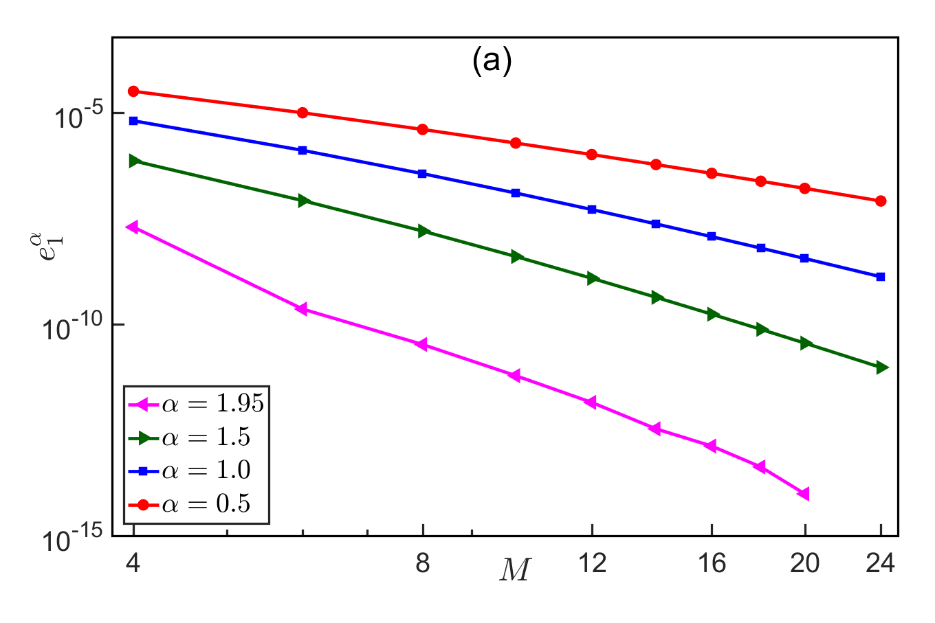
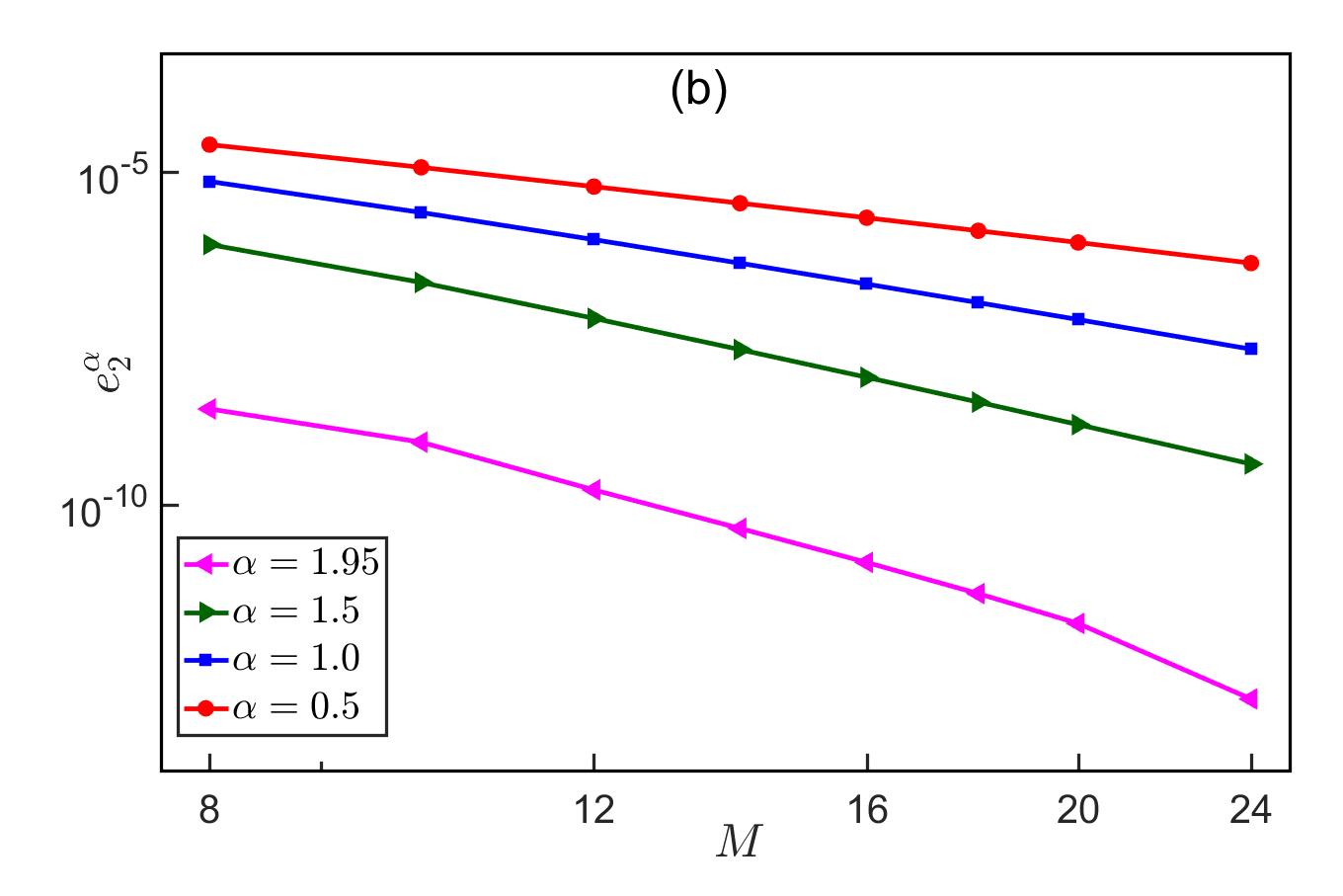
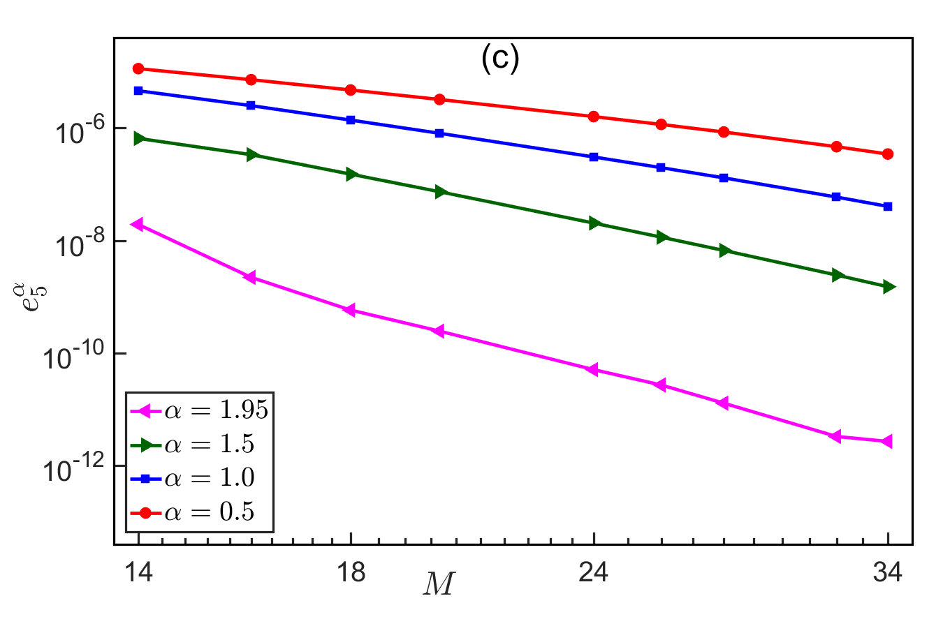
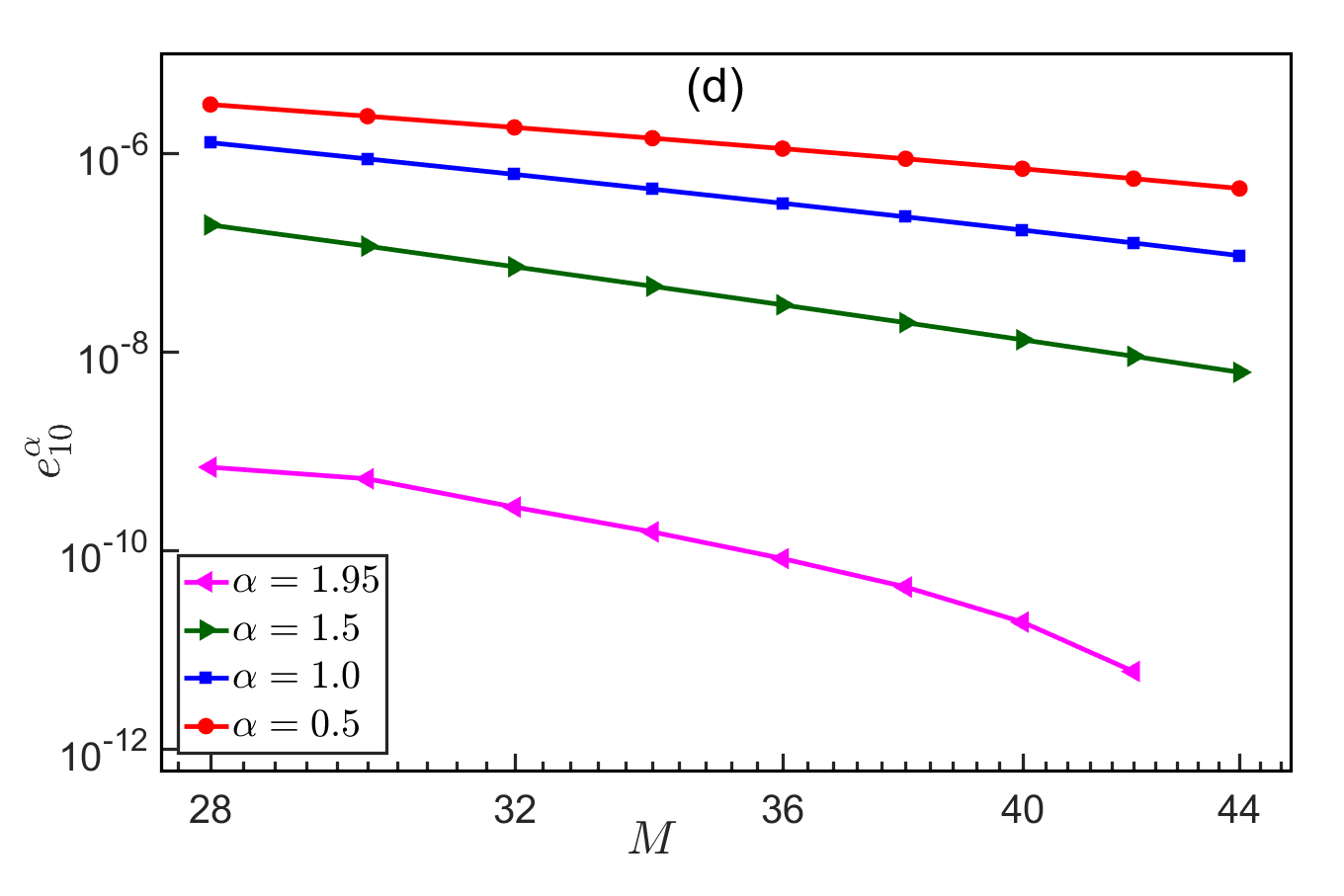
Figure 1: Convergence rates of computing different eigenvalues of (1.1) with $\Omega=(-1,1)$, $V(x)\equiv 0$ and different $\alpha$ by using our JSM (2.21) for: (a) the first eigenvalue $\lambda_{1}^{\alpha}$, (b) the second eigenvalue $\lambda_{2}^{\alpha}$, (c) the fifth eigenvalue $\lambda_{5}^{\alpha}$, and (d) the tenth eigenvalue $\lambda_{10}^{\alpha}$.

  

  

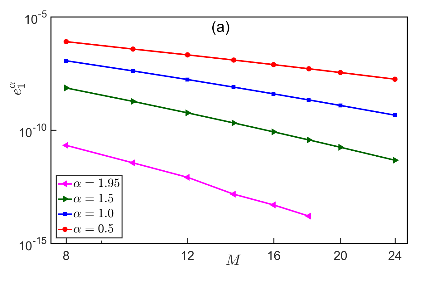
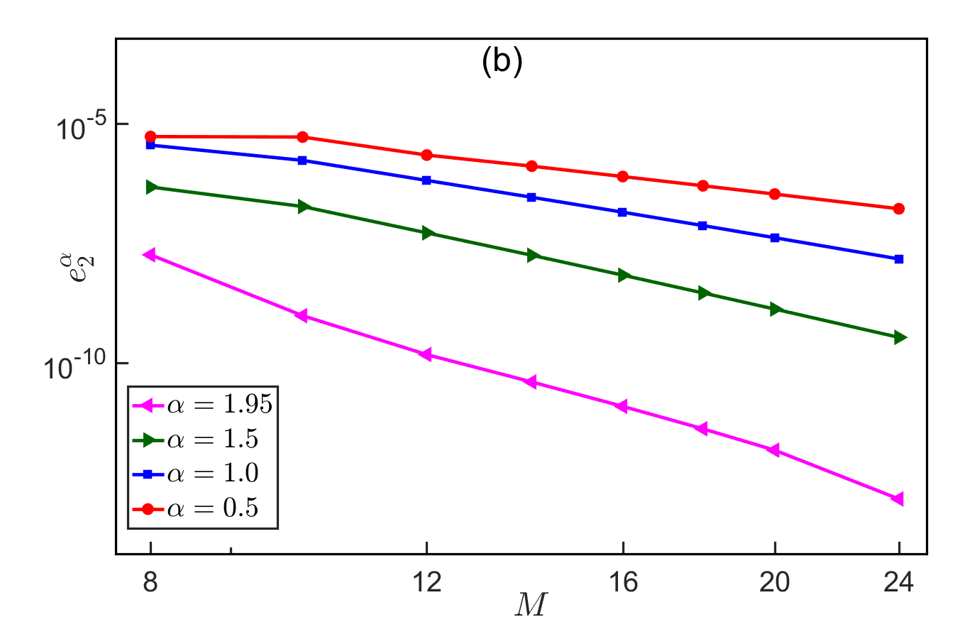
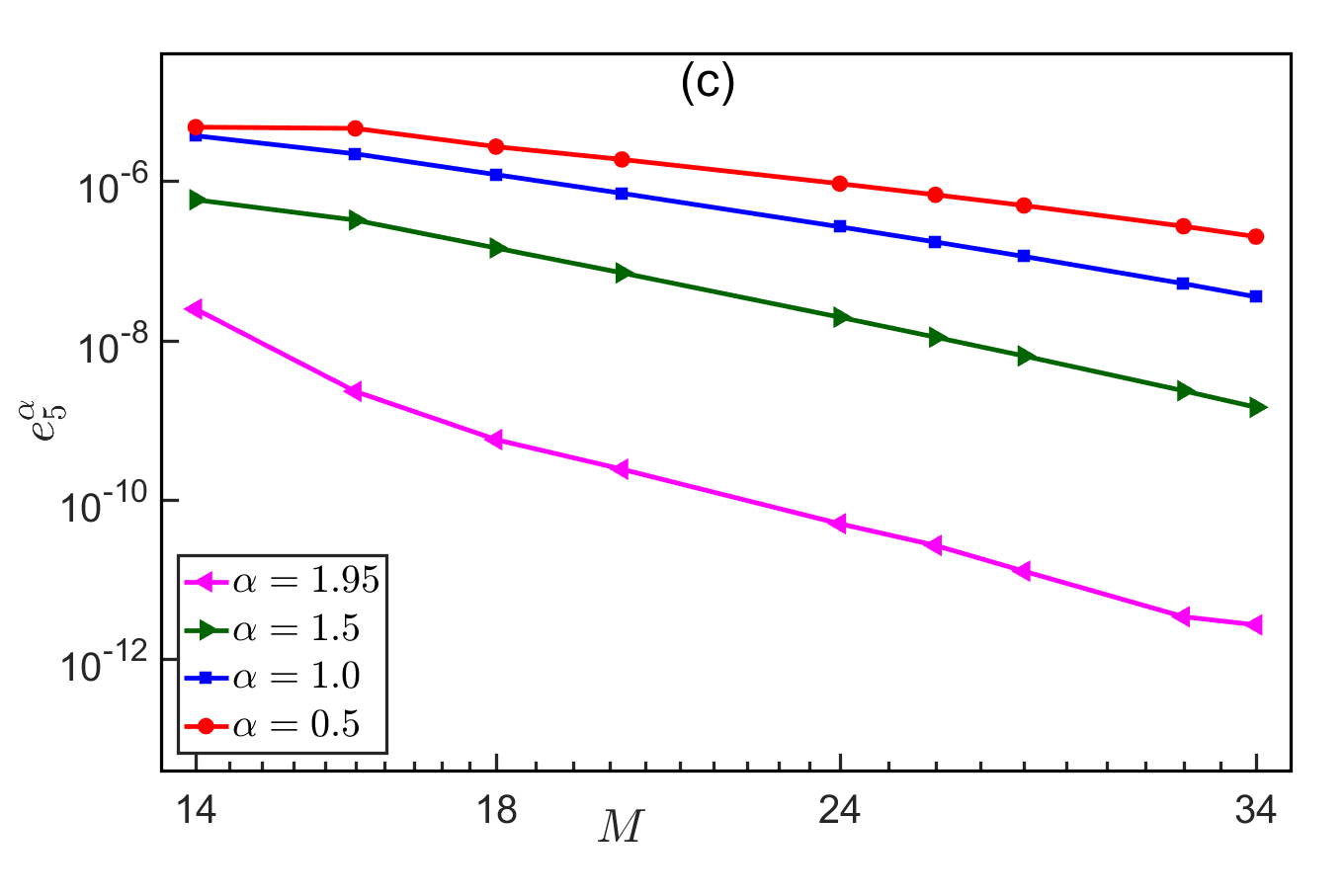
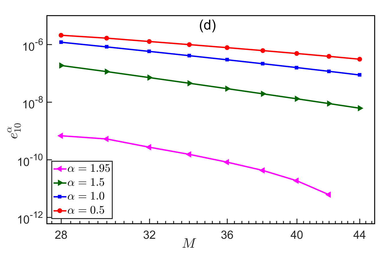
Figure 2: Convergence rates of computing different eigenvalues of (1.1) with $\Omega=(-1,1)$, $V(x)=\frac{x^{2}}{2}$ and different $\alpha$ by using our JSM (2.21) for: (a) the first eigenvalue $\lambda_{1}^{\alpha}$, (b) the second eigenvalue $\lambda_{2}^{\alpha}$, (c) the fifth eigenvalue $\lambda_{5}^{\alpha}$, and (d) the tenth eigenvalue $\lambda_{10}^{\alpha}$.

From Tabs. 1 & 2 and Figs. 1 & 2 and extensive additional results not shown here for brevity, we can draw the following conclusions: (i) For fixed DOF $M$ and $\alpha\in(0,2]$, the errors from our JSM (2.21) are significantly smaller than those from the FEM [35] and FDM [62, 19] (cf. Tabs. 1 & 2). (ii) Both the FEM [35] and FDM [62, 19] converge almost quadratically and linearly with respect to the DOF $M$ when $\alpha=2$ and $0<\alpha<2$, respectively (cf. Tabs. 1 & 2). (iii) Our JSM method (2.21) converges spectrally and super-linearly (or sub-spectrally) with respect to the DOF $M$ when $\alpha=2$ and $0<\alpha<2$, respectively (cf. Fig. 1 & 2). (iv) In Tab. 3, the numerical results reported by our JSM (2.21) have at least eight significant digits when the DOF $M\geq 160$, while the results by the asymptotic method in [63] have at most four significant digits even when the DOF $M=5000$! Thus our JSM method (2.21) is significantly accurate than those low-order numerical methods in the literatures for computing eigenvalues of the eigenvalue problem (1.1).

3.2 Resolution capacity (or trust region) test

In order to get reliable gaps and their distribution statistics, we have to calculate accurately and efficiently a very large number of eigenvalues, e.g. up to thousands or even millions eigenvalues. Specifically we need to make sure that the numerical errors are much smaller than the minimum gap of those gaps which are used to find numerically the distribution statistics. In general, to solve the eigenvalue problem (1.1) by a numerical method with a given DOF $M$, we can obtain $M$ approximate eigenvalues. A key question is that how many eigenvalues or what fraction among the $M$ approximate eigenvalues can be used to find numerically the distribution statistics, i.e. the errors to them are quite small. We remark here that for the Schrödinger operator, i.e. $\alpha=2$ in (1.1), by using a spectral method, it is proved that about $\frac{2}{\pi}$ fraction of the $M$ approximate eigenvalues is quite accurate (or the errors are quite small) [59]. To see whether this property is still valid for our JSM (2.21) for the FSO (1.1), Figure 3 displays the relative errors $e_{n,r}^{\alpha}$ ($n=1,2,\ldots,6400$) of (1.1) with $V(x)\equiv 0$ and different $\alpha$ by using our JSM (2.21), FEM [35] and FDM [62, 19] under the DOF $M=8192$.

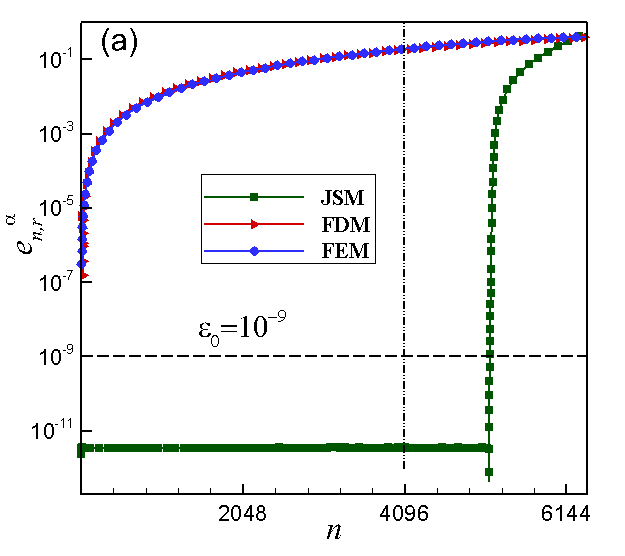
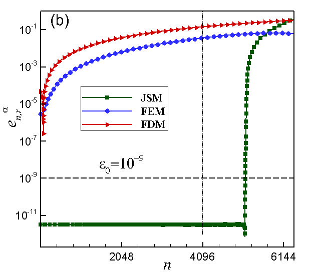
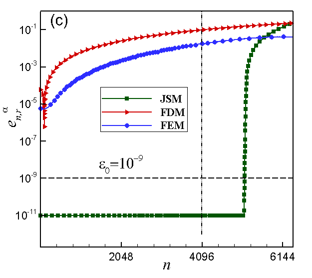
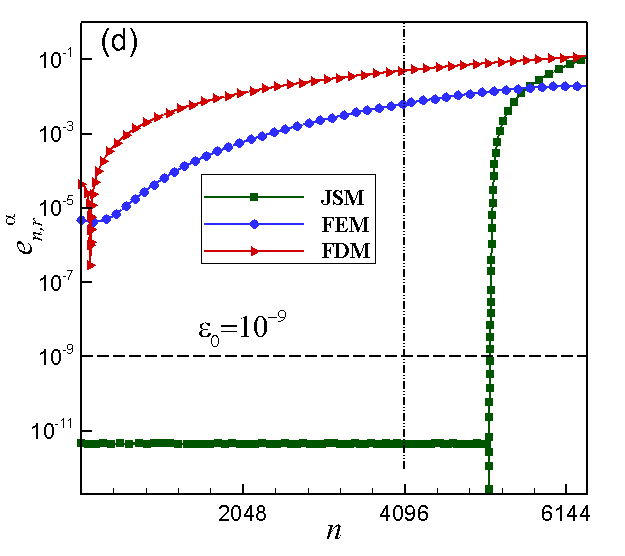
Figure 3: Relative errors of the first $6400$ eigenvalue, i.e. $e_{n,r}^{\alpha}$ ($n=1,2,\ldots,6400$) of (1.1) with $\Omega=(-1,1)$ and $V(x)\equiv 0$ by using our JSM (2.21), FEM [35] and FDM [62, 19] under the DOF $M=8192$ for: (a) $\alpha=1.95$, (b) $\alpha=1.5$, (c) $\alpha=1.0$, and (d) $\alpha=0.5$. A horizonal (dash) line with $\varepsilon_{0}:=10^{-9}$ and a vertical (dash) line with $n:=M/2$ are added in each sub-figure.

From Fig. 3, we can see that our JSM (2.21) is significantly better than FEM and FDM when a large number of eigenvalues are to be computed accurately. In fact, FEM and FDM can be used to compute the first a few eigenvalues of (1.1). However, when a large amount of eigenvalues are needed, one has to adapt a spectral method such as our JSM (2.21).

To quantify the resolution capacity of our JSM (2.21), Figure 4 displays the relative errors $e_{n,r}^{\alpha}$ ($n=1,2,\ldots,M$) of (1.1) with $V(x)\equiv 0$ and different $\alpha$ under different DOFs $M$, i.e. $M=512$, $2048$ and $8192$; and Figure 5 shows similar results when $V(x)=\frac{x^{2}}{2}$.

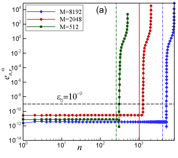
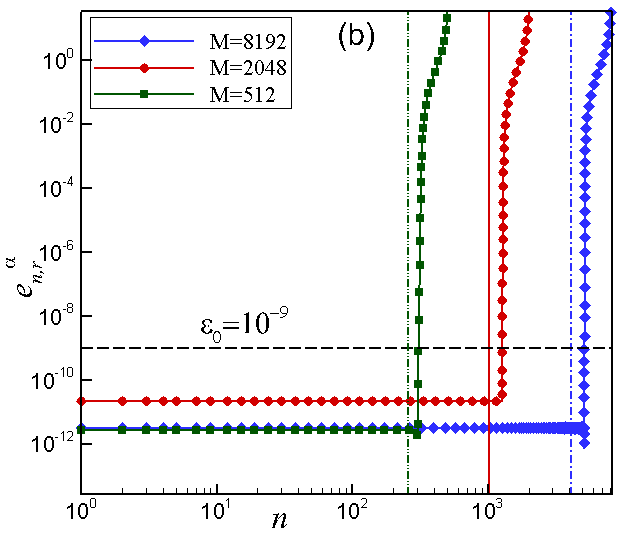
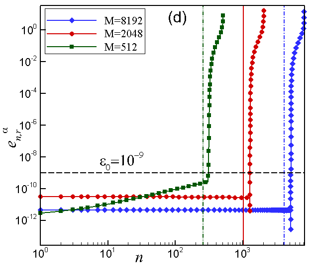
Figure 4: Relative errors of the eigenvalues of (1.1) with $\Omega=(-1,1)$ and $V(x)\equiv 0$ by using our JSM (2.21) under different DOFs $M$ for: (a) $\alpha=1.95$, (b) $\alpha=1.5$, (c) $\alpha=1.0$, and (d) $\alpha=0.5$. A horizonal (dash) line with $\varepsilon_{0}:=10^{-9}$ and vertical (dash) lines with $n:=M/2$ are added in each sub-figure.

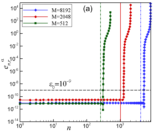
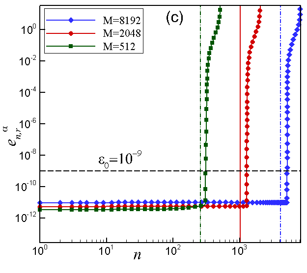
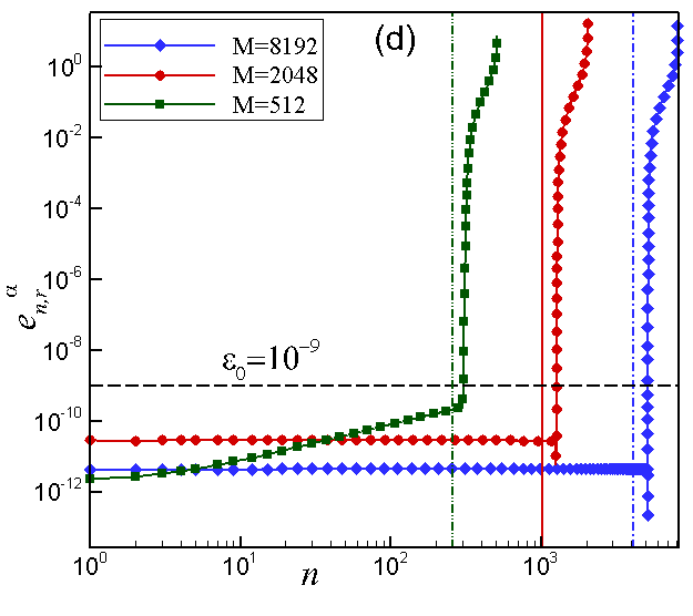
Figure 5: Relative errors of the eigenvalues of (1.1) with $\Omega=(-1,1)$ and $V(x)=\frac{x^{2}}{2}$ by using our JSM (2.21) under different DOFs $M$ for: (a) $\alpha=1.95$, (b) $\alpha=1.5$, (c) $\alpha=1.0$, and (d) $\alpha=0.5$. A horizonal (dash) line with $\varepsilon_{0}:=10^{-9}$ and vertical (dash) lines with $n:=M/2$ are added in each sub-figure.

From Figs. 4 & 5, we can see that our JSM (2.21) under a given DOF $M$ has the following resolution capacity (or trust region)

$$e_{n,r}^{\alpha}:=\frac{\left|\lambda_{n}^{\alpha}-\lambda_{n,M}^{\alpha}\right|}{\lambda_{n}^{\alpha}}\leq\varepsilon_{0}:=10^{-9},\qquad n=1,2,\ldots,c_{r}M,\qquad\hbox{with}\quad c_{r}\approx\frac{2}{\pi}>\frac{1}{2}.$$ (3.2)

4 Numerical results of FSO in 1D without potential

In this section, we report numerical results on eigenvalues of (1.1) with $\Omega=(-1,1)$ and $V(x)\equiv 0$ by using our JSM (2.21) under the DOF $M=8192$. All results are based on the first $4096$ eigenvalues, i.e. we use half of the eigenvalues obtained numerically to present the results and to calculate distribution statistics.

4.1 Eigenvalues and their approximations

Figure 6a plots eigenvalues $\lambda_{n}^{\alpha}$ ($n=1,2,\ldots$) and their leading order approximations as $\lambda_{n}^{\alpha}\approx\tilde{\lambda}_{n}^{\alpha}:=\left(\frac{n\pi}{2}\right)^{\alpha}$ ($n=1,2,\ldots$), while $\tilde{\lambda}_{n}^{\alpha}$ ($n=1,2,\ldots$) are the eigenvalues of the local fractional Laplacian operator on $\Omega=(-1,1)$ with homogeneous Dirichlet boundary condition [8]. Figure 6b displays the relative errors of the eigenvalues and their leading order approximations, i.e. $\tilde{e}_{n,r}^{\alpha}:=\left(\tilde{\lambda}_{n}^{\alpha}-\lambda_{n}^{\alpha}\right)/\tilde{\lambda}_{n}^{\alpha}$, which immediately suggests a high order approximation at $\lambda_{n}^{\alpha}\approx\hat{\lambda}_{n}^{\alpha}:=\tilde{\lambda}_{n}^{\alpha}\left(1-\frac{C_{3}^{\alpha}}{n}\right)$ ($n=1,2,\ldots$). By fitting our numerical results, we can obtain numerically $C_{3}^{\alpha}=\frac{\alpha(2-\alpha)}{4}$ which is plotted in Figure 6c. Finally Figure 6d displays the absolute errors of the eigenvalues and their high order approximations, i.e. $\tilde{e}_{n}^{\alpha}:=\left|\lambda_{n}^{\alpha}-\hat{\lambda}_{n}^{\alpha}\right|$.

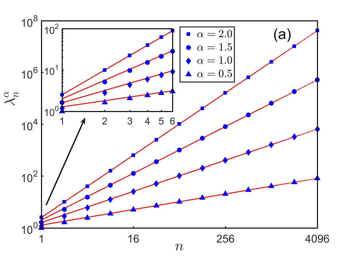
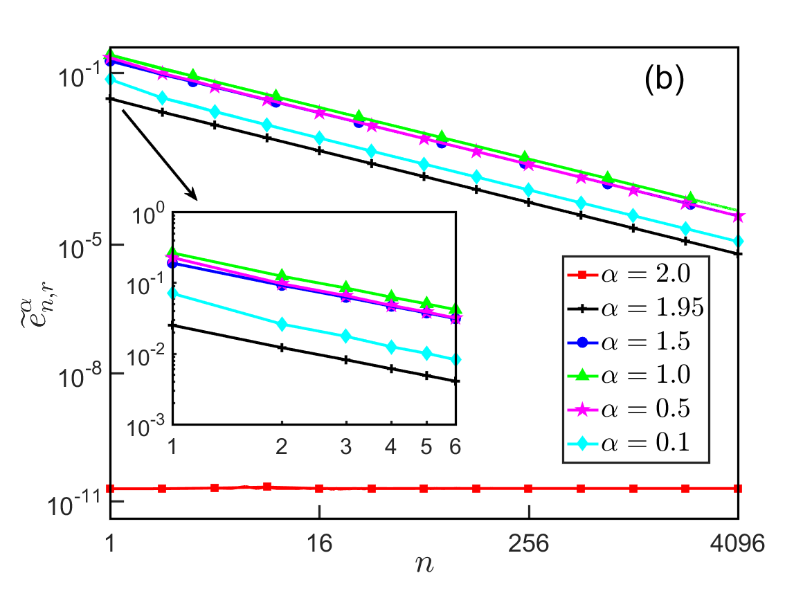
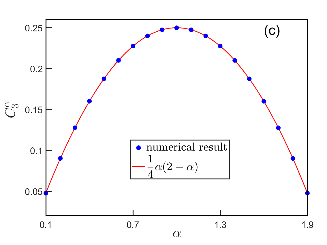
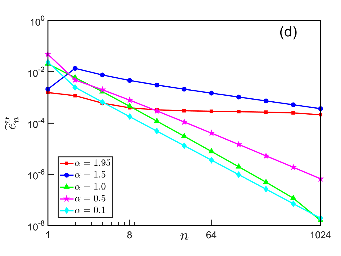
Figure 6: (a) Eigenvalues $\lambda_{n}^{\alpha}$ ($n=1,2,\ldots,4096$) of (1.1) with $\Omega=(-1,1)$ and $V(x)\equiv 0$ for different $\alpha$ (symbols denote numerical results and solids lines are from the leading order approximation $\tilde{\lambda}_{n}^{\alpha}=\left(\frac{n\pi}{2}\right)^{\alpha}$); (b) Relative errors $\tilde{e}_{n,r}^{\alpha}=\left(\tilde{\lambda}_{n}^{\alpha}-\lambda_{n}^{\alpha}\right)/\tilde{\lambda}_{n}^{\alpha}$ (symbols denote numerical results and solids lines are from fitting formula $C_{3}^{\alpha}n^{-1}$ when $n\gg 1$); (c) Fitting results for $C_{3}^{\alpha}$; and (d) absolute errors $\tilde{e}_{n}^{\alpha}=\left|\lambda_{n}^{\alpha}-\hat{\lambda}_{n}^{\alpha}\right|$ with $\hat{\lambda}_{n}^{\alpha}=\tilde{\lambda}_{n}^{\alpha}\left(1-C_{3}^{\alpha}\,n^{-1}\right)$.

From Fig. 6, we can obtain numerically the following approximations of the eigenvalues of (1.1) with $\Omega=(-1,1)$ and $V(x)\equiv 0$ as

$$\lambda_{n}^{\alpha}=\hat{\lambda}_{n}^{\alpha}+O(n^{\alpha-2})=\tilde{\lambda}_{n}^{\alpha}\left[1-\frac{\alpha(2-\alpha)}{4n}+O(n^{-2})\right],\quad n=1,2,\ldots\;,$$ (4.1)

where

$$\tilde{\lambda}_{n}^{\alpha}=\left(\frac{n\pi}{2}\right)^{\alpha},\quad\hat{\lambda}_{n}^{\alpha}=\left(\frac{n\pi}{2}\right)^{\alpha}-\left(\frac{\pi}{2}\right)^{\alpha}\frac{\alpha(2-\alpha)}{4}n^{\alpha-1}=\tilde{\lambda}_{n}^{\alpha}\left[1-\frac{\alpha(2-\alpha)}{4n}\right],\quad n\geq 1,\quad 0<\alpha\leq 2.\quad$$ (4.2)

Combining (4.1) and Lemma 2.1, we can immediately obtain the conclusion (1.16).

To demonstrate high accuracy of our numerical method, Table 4 lists eigenvalues of (1.1) with $\Omega=(-1,1)$ and $V(x)\equiv 0$ for different $\alpha$.

	$\alpha=0.1$	$\alpha=0.5$	$\alpha=1.0$	$\alpha=1.5$	$\alpha=1.95$	$\alpha=2.0$
$\lambda_{1}^{\alpha}$	0.9725944	0.9701654	1.157773883	1.5975035456	2.35198053244	2.4674011002
$\lambda_{2}^{\alpha}$	1.0921964	1.6015377	2.754754742	5.0597599283	9.20812426623	9.8696044010
$\lambda_{3}^{\alpha}$	1.1473224	2.0288210	4.316801066	9.5943057675	20.3833201062	22.206609902
$\lambda_{4}^{\alpha}$	1.1868395	2.3871563	5.892147470	15.018786212	35.7934316323	39.478417604
$\lambda_{5}^{\alpha}$	1.2165513	2.6947426	7.460175739	21.189425897	55.3737634238	61.685027506
$\lambda_{6}^{\alpha}$	1.2412799	2.9728959	9.032852690	28.035207791	79.0793754673	88.826439609
$\lambda_{7}^{\alpha}$	1.2619743	3.2256090	10.60229309	35.488011031	106.871259423	120.90265391
$\lambda_{8}^{\alpha}$	1.2801923	3.4610502	12.17411826	43.507108689	138.718756729	157.91367041
$\lambda_{9}^{\alpha}$	1.2961956	3.6805940	13.74410905	52.051027490	174.594065184	199.85948912
$\lambda_{10}^{\alpha}$	1.3107082	3.8884472	15.31555499	61.092457389	214.473975149	246.74011002
$\lambda_{20}^{\alpha}$	1.4082270	5.5522311	31.02330309	174.43784577	829.684155066	986.96044010
$\lambda_{40}^{\alpha}$	1.5111219	7.8894197	62.43917339	495.95713648	3207.64320222	3947.8417604
$\lambda_{60}^{\alpha}$	1.5742803	9.6777480	93.85508924	912.11187382	7073.79138904	8882.6439609

Table 4: Eigenvalues of (1.1) with $\Omega=(-1,1)$ and $V(x)\equiv 0$ for different $\alpha$.

4.2 Asymptotic behaviour of different gaps

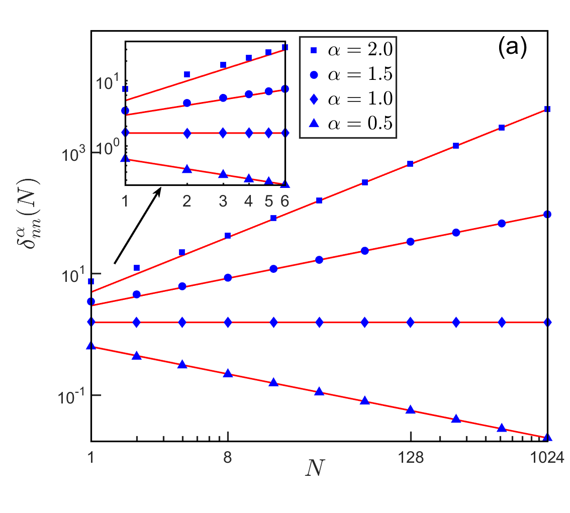
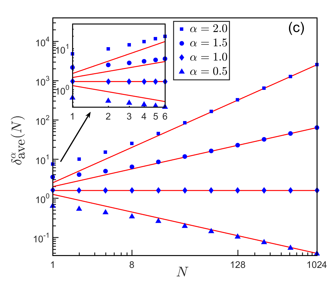
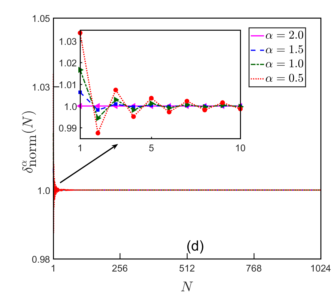
Figure 7: Different eigenvalue gaps of (1.1) with $\Omega=(-1,1)$, $V(x)\equiv 0$ and different $\alpha$ for (symbols denote numerical results and solids lines are from fitting formula when $N\gg 1$): (a) the nearest neighbour gaps $\delta_{\rm nn}^{\alpha}(N)$, (b) the minimum gaps $\delta_{\textrm{min}}^{\alpha}(N)$, (c) the average gaps $\delta_{\textrm{ave}}^{\alpha}(N)$, and (d) the normalized gaps $\delta_{\rm norm}^{\alpha}(N)$.

Figure 7 plots different eigenvalue gaps of (1.1) with $\Omega=(-1,1)$, $V(x)\equiv 0$ and different $\alpha$. From Fig. 7, we can draw the following conclusions based on our numerical results: (i) the nearest neighbour gaps $\delta_{\rm nn}^{\alpha}(N)$ increase and decrease with respect to $N$ when $1<\alpha\leq 2$ and $0<\alpha<1$, respectively; and they are almost constant when $\alpha=1$ (cf. Fig. 7a). (ii) The minimum gaps $\delta_{\textrm{min}}^{\alpha}(N)$ are almost constants and decrease with respect to $N$ when $1\leq\alpha\leq 2$ and $0<\alpha<1$, respectively (cf. Fig. 7b). (iii) The average gaps $\delta_{\textrm{ave}}^{\alpha}(N)$ increase and decrease with respect to $N$ when $1<\alpha\leq 2$ and $0<\alpha<1$, respectively; and they are almost constant when $\alpha=1$ (cf. Fig. 7c). (iv) The normalized gaps $\delta_{\rm norm}^{\alpha}(N)\approx 1$ when $N\gg 1$ (cf. Fig. 7d).

In fact, based on the numerical asymptotic approximation (4.1), we can formally obtain the following approximation of the nearest neighbour gaps as

$$\delta_{\rm nn}^{\alpha}(N) = \lambda_{N+1}^{\alpha}-\lambda_{N}^{\alpha}\approx\hat{\lambda}_{N+1}^{\alpha}-\hat{\lambda}_{N}^{\alpha}$$ (4.3)

$$= \left(\frac{(N+1)\pi}{2}\right)^{\alpha}-\left(\frac{\pi}{2}\right)^{\alpha}\frac{\alpha(2-\alpha)}{4}(N+1)^{\alpha-1}-\left(\frac{N\pi}{2}\right)^{\alpha}+\left(\frac{\pi}{2}\right)^{\alpha}\frac{\alpha(2-\alpha)}{4}N^{\alpha-1}$$

$$= \left(\frac{\pi}{2}\right)^{\alpha}\left[(N+1)^{\alpha}-N^{\alpha}-\frac{\alpha(2-\alpha)}{4}\left((N+1)^{\alpha-1}-N^{\alpha-1}\right)\right]$$

$$= \left(\frac{\pi}{2}\right)^{\alpha}\left[N^{\alpha}\left(\left(1+\frac{1}{N}\right)^{\alpha}-1\right)-\frac{\alpha(2-\alpha)}{4}N^{\alpha-1}\left(\left(1+\frac{1}{N}\right)^{\alpha-1}-1\right)\right]$$

$$= \left(\frac{\pi}{2}\right)^{\alpha}\left[N^{\alpha}\left(\frac{\alpha}{N}+\frac{\alpha(\alpha-1)}{N^{2}}+O(N^{-3})\right)-\frac{\alpha(2-\alpha)}{4}N^{\alpha-1}\left(\frac{\alpha-1}{N}+O(N^{-2})\right)\right]$$

$$= \left(\frac{\pi}{2}\right)^{\alpha}\left[\alpha N^{\alpha-1}+\frac{\alpha(\alpha-1)(2+\alpha)}{4}N^{\alpha-2}+O(N^{\alpha-3})\right],\qquad N=1,2,\ldots\;.$$

Again, this asymptotic results also confirm that the nearest neighbour gaps $\delta_{\rm nn}^{\alpha}(N)$ increase and decrease with respect to $N$ when $1<\alpha\leq 2$ and $0<\alpha<1$, respectively; and they are almost constant when $\alpha=1$.

Based on the asymptotic results (4.3) and the numerical results in Fig. 7b, we can conclude that

$$\delta_{\rm min}^{\alpha}(N)=\left\{\begin{array}[]{ll}\delta_{\rm nn}^{\alpha}(1)=\lambda_{2}^{\alpha}-\lambda_{1}^{\alpha},&1<\alpha<2,\\ \approx\delta_{\rm nn}^{\alpha}(1)=\lambda_{2}^{\alpha}-\lambda_{1}^{\alpha},&\alpha=1,\\ \delta_{\rm nn}^{\alpha}(N)\approx\alpha\left(\frac{\pi}{2}\right)^{\alpha}N^{\alpha-1},&0<\alpha<1.\\ \end{array}\right.\qquad N=1,2,\ldots\;.$$ (4.4)

Again, these asymptotic results suggest that the minimum gaps $\delta_{\textrm{min}}^{\alpha}(N)$ are almost constants and decrease with respect to $N$ when $1\leq\alpha\leq 2$ and $0<\alpha<1$, respectively.

Similarly, we have the asymptotic results for the average gaps as

$$\delta_{\rm ave}^{\alpha}(N) = \frac{\lambda_{N+1}^{\alpha}-\lambda_{1}^{\alpha}}{N}\approx\frac{\hat{\lambda}_{N+1}^{\alpha}-\lambda_{1}^{\alpha}}{N}$$ (4.5)

$$= \frac{1}{N}\left[\left(\frac{(N+1)\pi}{2}\right)^{\alpha}-\left(\frac{\pi}{2}\right)^{\alpha}\frac{\alpha(2-\alpha)}{4}(N+1)^{\alpha-1}-\lambda_{1}^{\alpha}\right]$$

$$= \left(\frac{\pi}{2}\right)^{\alpha}\left[N^{\alpha-1}\left(1+\frac{1}{N}\right)^{\alpha}-\frac{\alpha(2-\alpha)}{4}N^{\alpha-2}\left(1+\frac{1}{N}\right)^{\alpha-1}-\lambda_{1}^{\alpha}\left(\frac{2}{\pi}\right)^{\alpha}N^{-1}\right]$$

$$= \left(\frac{\pi}{2}\right)^{\alpha}\left[N^{\alpha-1}+\alpha N^{\alpha-2}-\frac{\alpha(2-\alpha)}{4}N^{\alpha-2}-\lambda_{1}^{\alpha}\left(\frac{2}{\pi}\right)^{\alpha}N^{-1}+O(N^{\alpha-3})\right]$$

$$= \left(\frac{\pi}{2}\right)^{\alpha}\left[N^{\alpha-1}+\frac{\alpha(2+\alpha)}{4}N^{\alpha-2}-\lambda_{1}^{\alpha}\left(\frac{2}{\pi}\right)^{\alpha}N^{-1}+O(N^{\alpha-3})\right],\qquad N=1,2,\ldots\;.$$

Thus when $1<\alpha<2$, we have

$$\delta_{\rm ave}^{\alpha}(N)=\left(\frac{\pi}{2}\right)^{\alpha}\left[N^{\alpha-1}+\frac{\alpha(2+\alpha)}{4}N^{\alpha-2}+O(N^{-1})\right],\qquad N=1,2,\ldots\;,$$ (4.6)

and when $0<\alpha<1$, we have

$$\delta_{\rm ave}^{\alpha}(N)=\left(\frac{\pi}{2}\right)^{\alpha}\left[N^{\alpha-1}-\lambda_{1}^{\alpha}\left(\frac{2}{\pi}\right)^{\alpha}N^{-1}+O(N^{\alpha-2})\right],\qquad N=1,2,\ldots\;,$$ (4.7)

and when $\alpha=1$, we get

$$\delta_{\rm ave}^{\alpha}(N)=\frac{\pi}{2}\left[1+\left(\frac{3}{4}-\frac{2}{\pi}\lambda_{1}^{\alpha=1}\right)N^{-1}+O(N^{-2})\right],\qquad N=1,2,\ldots\;.$$ (4.8)

Again, these asymptotic results suggest that the average gaps $\delta_{\textrm{ave}}^{\alpha}(N)$ increase and decrease with respect to $N$ when $1<\alpha\leq 2$ and $0<\alpha<1$, respectively; and they are almost constants when $\alpha=1$ (cf. Fig. 7c).

Based on the asymptotic results of the eigenvalue $\lambda_{n}^{\alpha}$ in (4.1), noticing (1.8)-(1.10), we can get the asymptotic results for the normalized gaps as

$$\delta_{\rm norm}^{\alpha}(N) = \frac{2}{\pi}\left[\left(\lambda_{N+1}^{\alpha}\right)^{1/\alpha}-\left(\lambda_{N}^{\alpha}\right)^{1/\alpha}\right]$$ (4.9)

$$= (N+1)\left(1-\frac{\alpha(2-\alpha)}{4(N+1)}+O((N+1)^{-2})\right)^{1/\alpha}-N\left(1-\frac{\alpha(2-\alpha)}{4N}+O(N^{-2})\right)^{1/\alpha}$$

$$= N+1-\frac{2-\alpha}{4}-\frac{\tilde{C}}{N+1}+O((N+1)^{-2})-N+\frac{2-\alpha}{4}+\frac{\tilde{C}}{N}-O(N^{-2})$$

$$= 1+\frac{\tilde{C}}{N(N+1)}+O(N^{-3}),\qquad N=1,2,\ldots\;,$$

where $\tilde{C}$ is a constant. Again, this asymptotic result suggests that the normalized gaps $\delta_{\textrm{norm}}^{\alpha}(N)\approx 1$ when $N\gg 1$ (cf. Fig. 7d).

Finally, combining (4.3), (4.4), (4.6), (4.7), (4.8), (4.9) and (2.3), we can get the conjecture (1.17) stated in Section 1.

4.3 The gap distribution statistics

Figure 8 displays the histogram of the normalized gaps $\{\delta_{\rm norm}^{\alpha}(n)\ |\ 1\leq n\leq N=4096\}$ defined in (4.9) for (1.1) with $\Omega=(-1,1)$, $V(x)\equiv 0$ and different $\alpha$.

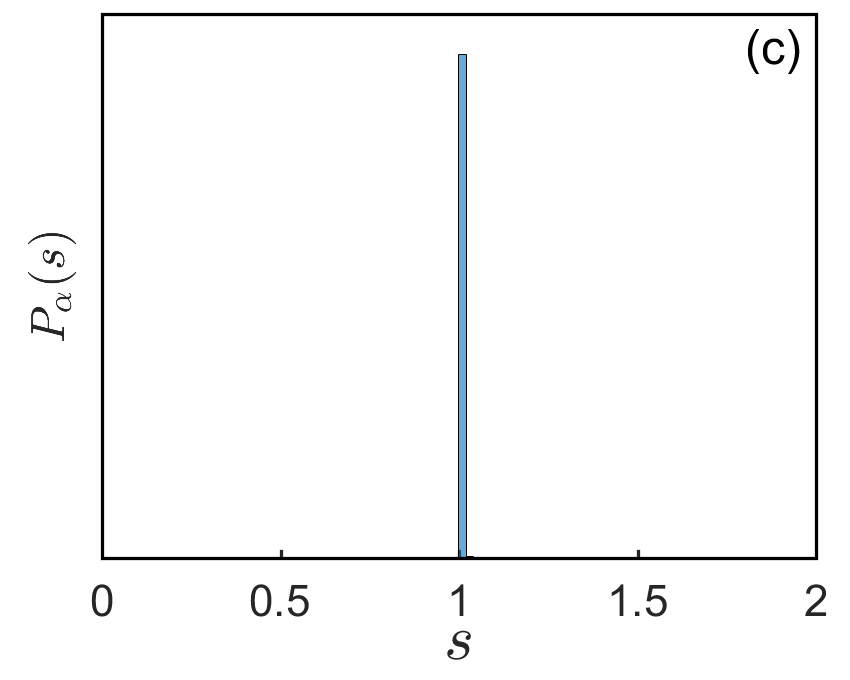
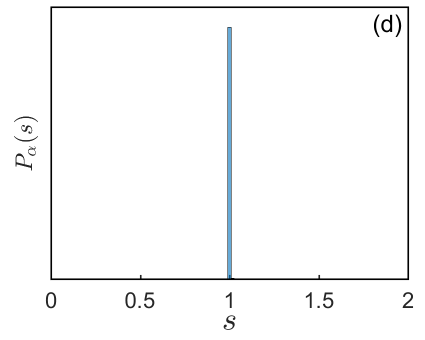
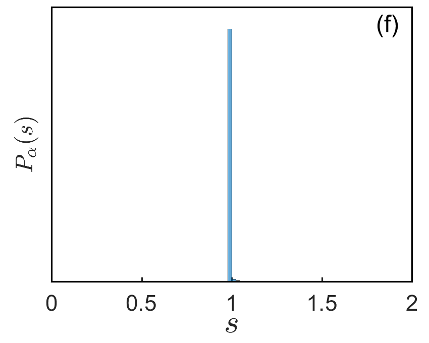
Figure 8: The histogram of the normalized gaps $\{\delta_{\rm norm}^{\alpha}(n)\ |\ 1\leq n\leq N=4096\}$ of (1.1) with $\Omega=(-1,1)$ and $V(x)\equiv 0$ for different $\alpha$: (a) $\alpha=2.0$, (b) $\alpha=1.9$, (c) $\alpha=\sqrt{3}$, (d) $\alpha=1.5$, (e) $\alpha=1.0$, and (f) $\alpha=0.5$.

From Fig. 8, we can conclude that the gaps distribution statistics of (1.1) with $V(x)\equiv 0$ is $P_{\alpha}(s)=\delta(s-1)$ for $0<\alpha\leq 2$.

4.4 Eigenfunctions and their singularity characteristics

  

  

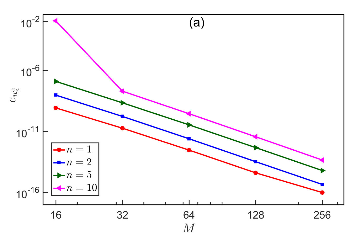
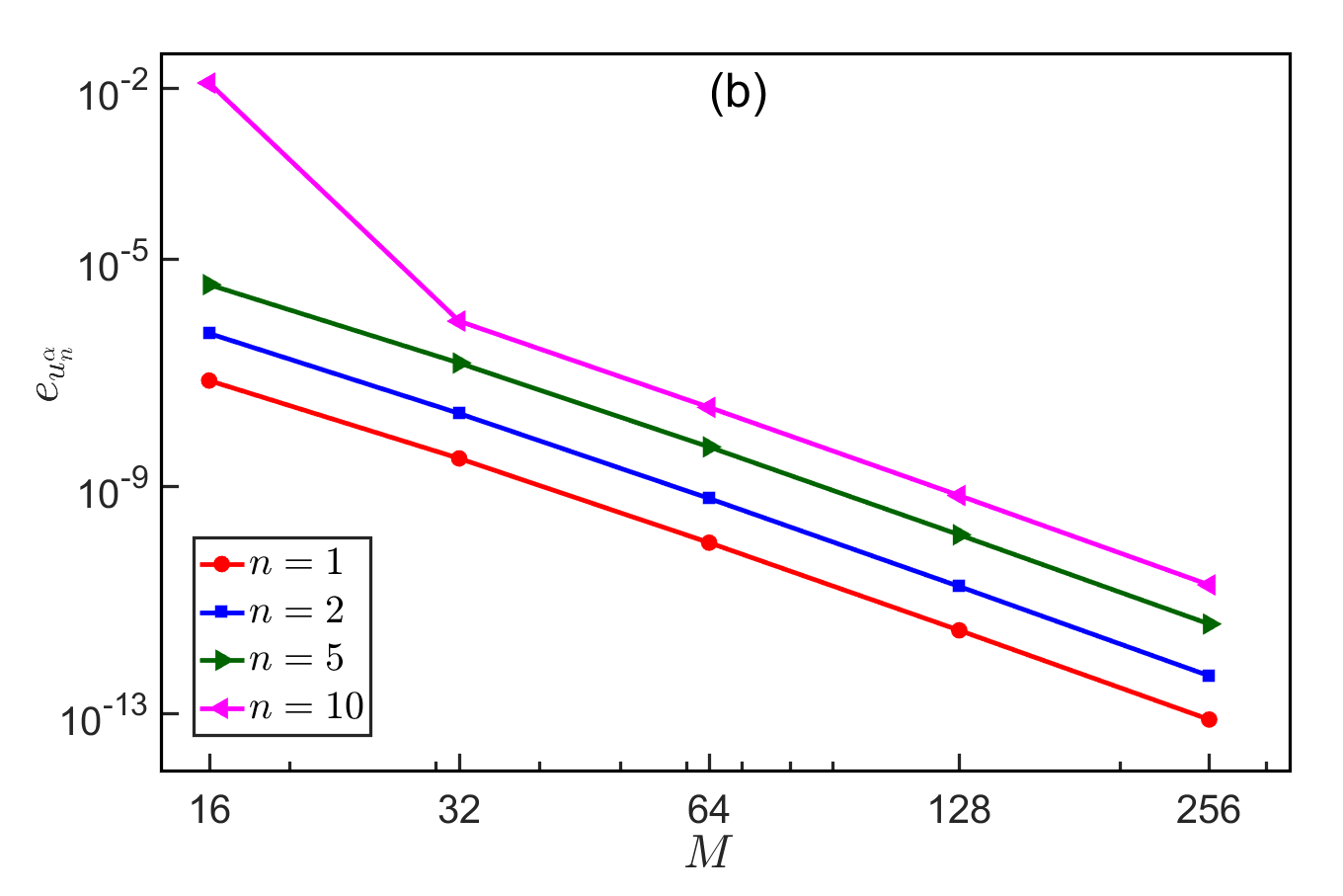
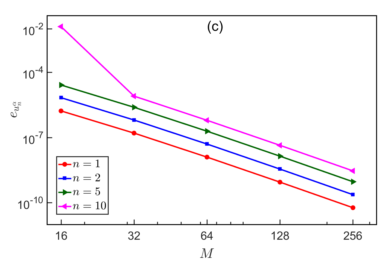
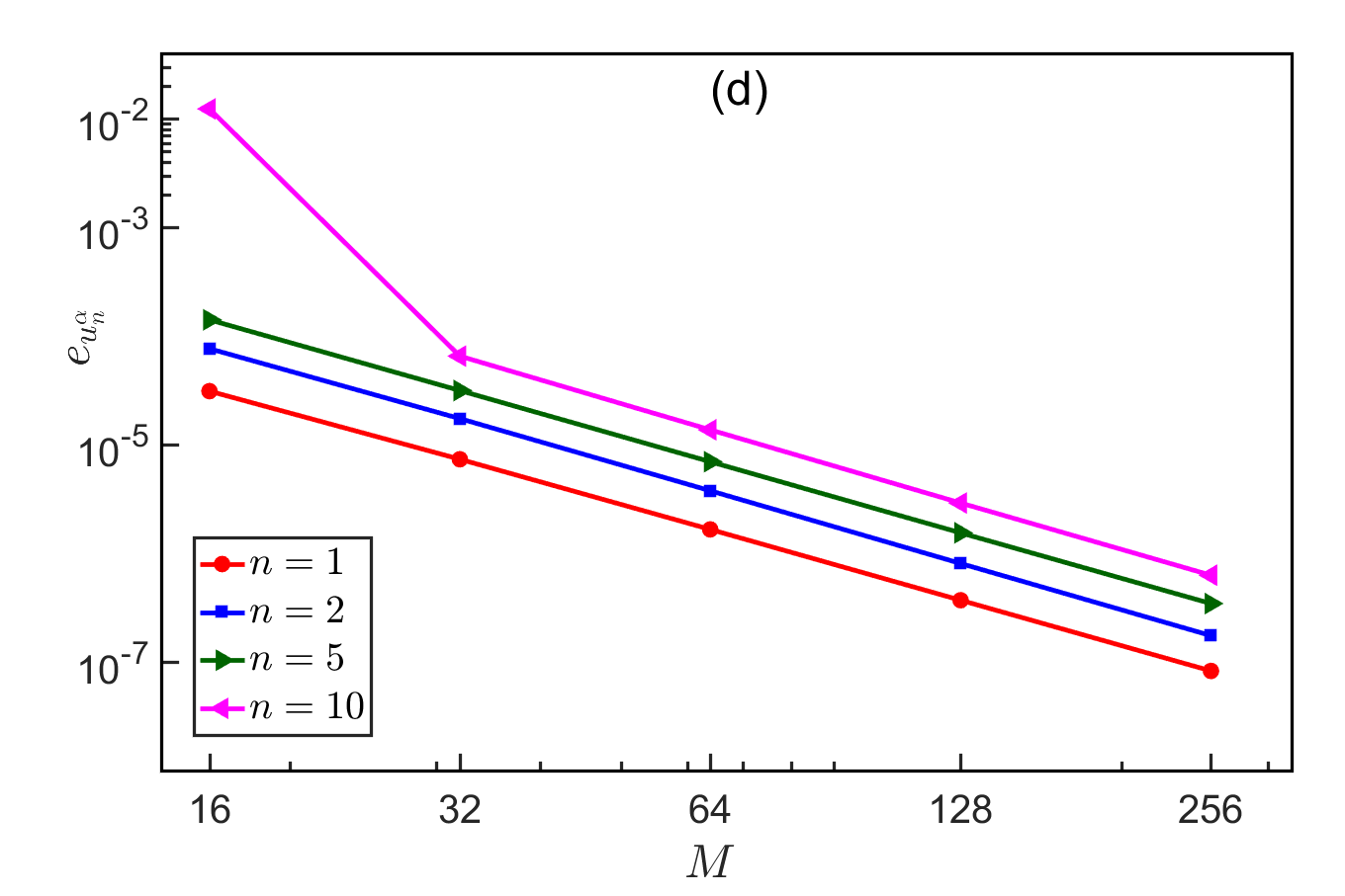
Figure 9: Convergence rates of computing different eigenfunctions of (1.1) with $\Omega=(-1,1)$, $V(x)\equiv 0$ and different $\alpha$ by using our JSM (2.21) for: (a) the first eigenfunction $u_{1}^{\alpha}$, (b) the second eigenfunction $u_{2}^{\alpha}$, (c) the fifth eigenfunction $u_{5}^{\alpha}$, and (d) the tenth eigenfunction $u_{10}^{\alpha}$.

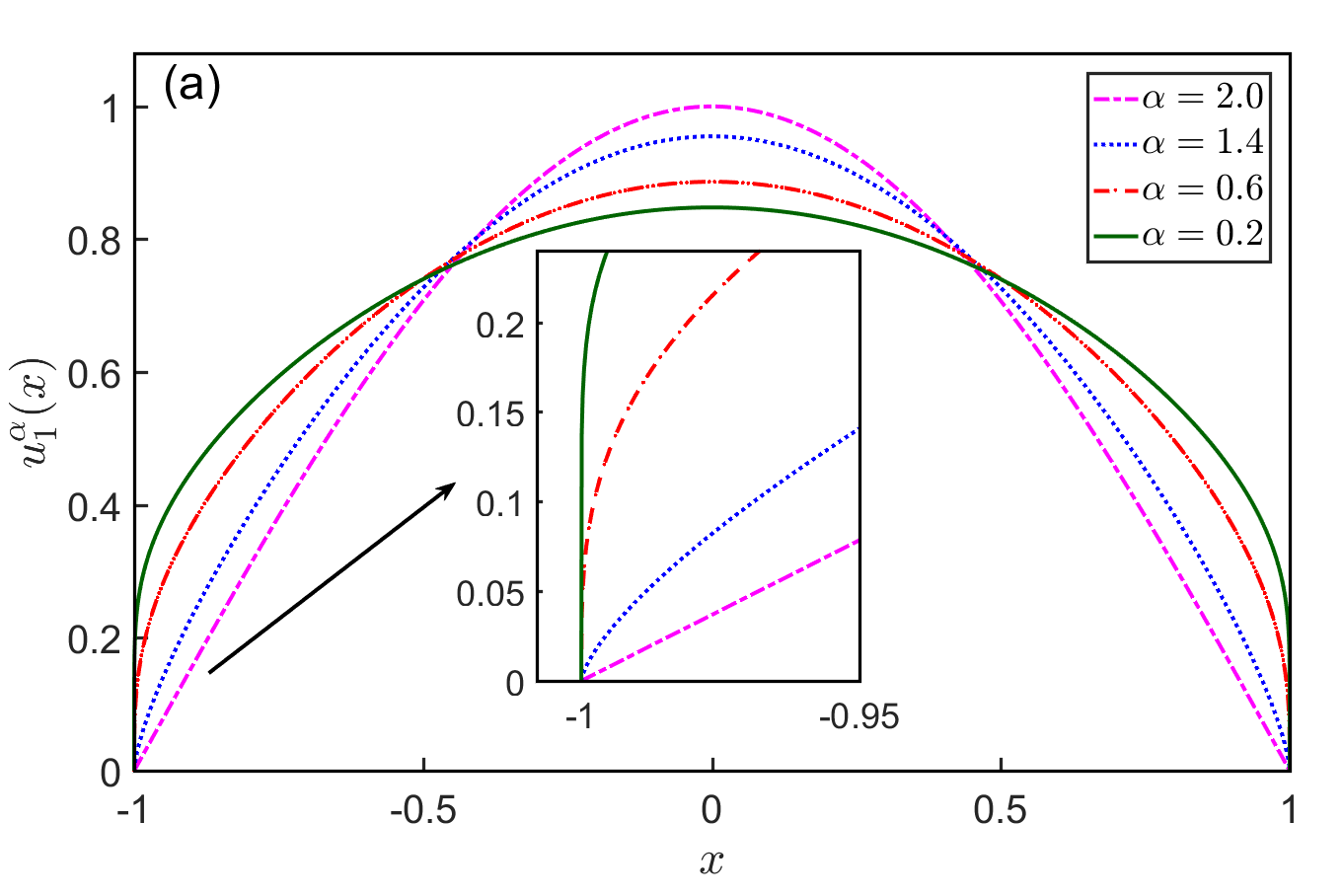
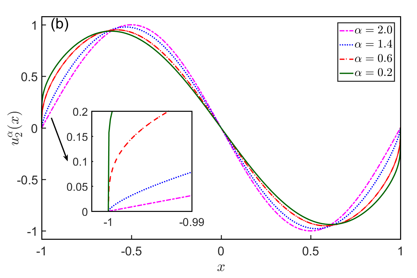
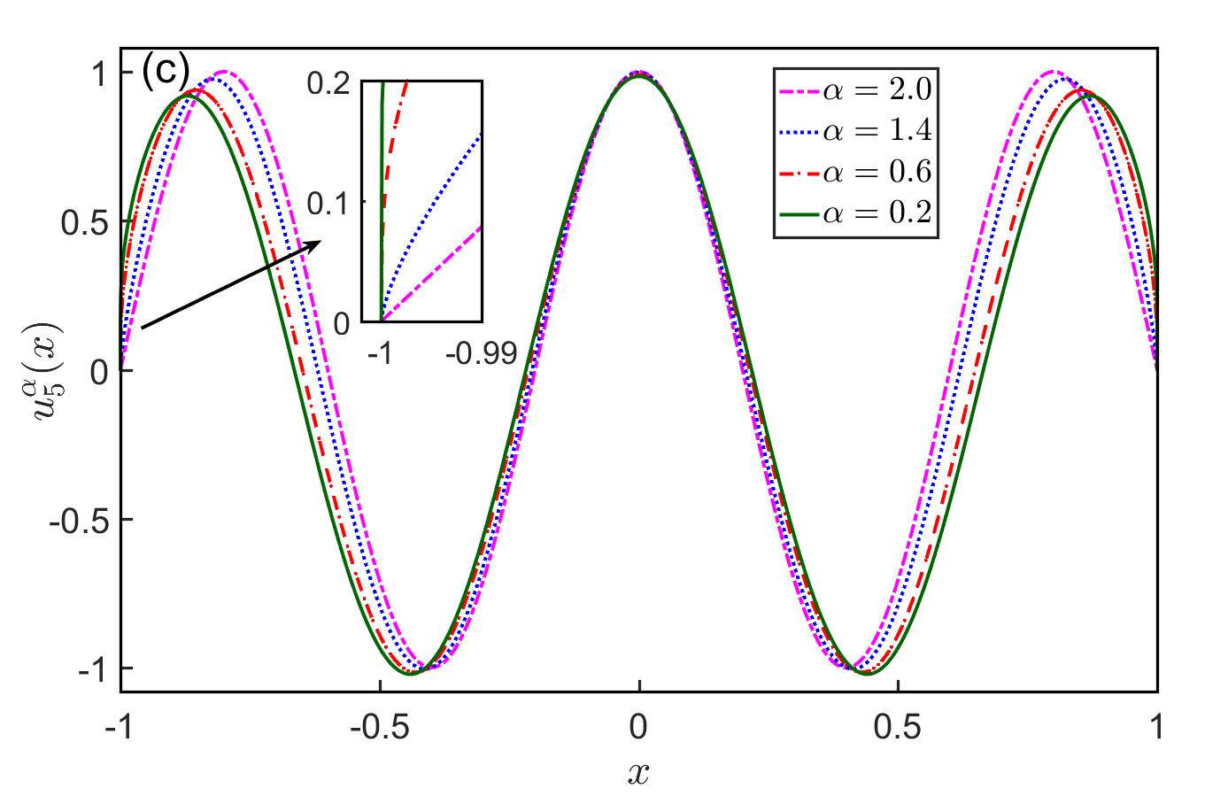
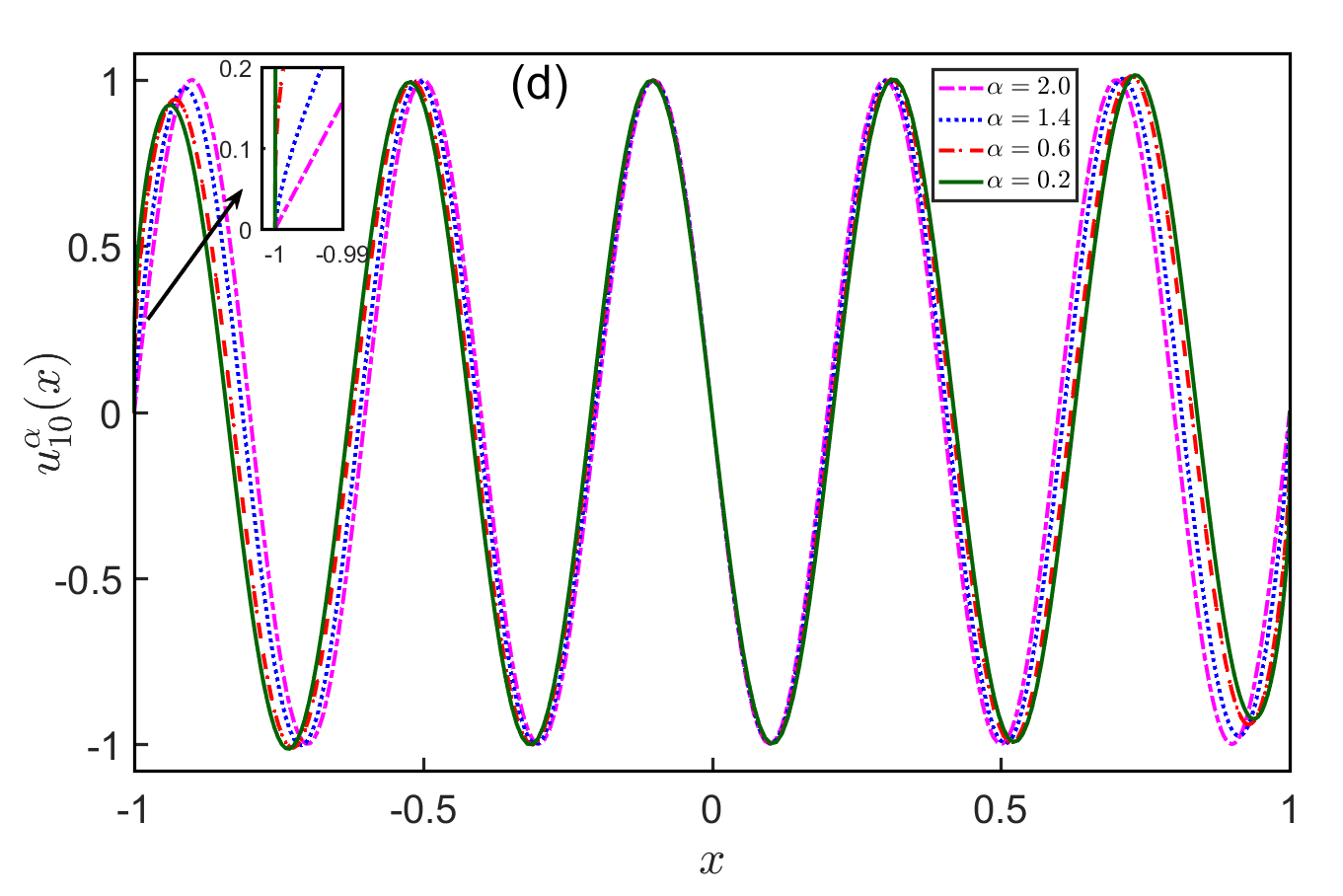
Figure 10: Plots of different eigenfunctions of (1.1) with $\Omega=(-1,1)$, $V(x)\equiv 0$ and different $\alpha$ for: (a) the first eigenfunction $u_{1}^{\alpha}(x)$, (b) the second eigenfunction $u_{2}^{\alpha}(x)$, (c) the fifth eigenfunction $u_{5}^{\alpha}(x)$, and (d) the tenth eigenfunction $u_{10}^{\alpha}(x)$.

Denote $u_{n}^{\alpha}(x)$ be the eigenfunction satisfying $\|u_{n}^{\alpha}\|_{L^{2}(\Omega)}=1$ and $\left.\frac{du_{n}^{\alpha}(x)}{dx}\right|_{x=-1}>0$, which corresponds to the eigenvalue $\lambda_{n}^{\alpha}$ ($n=1,2,\ldots$) of (1.1) with $\Omega=(-1,1)$ and $V(x)\equiv 0$. The ‘exact’ eigenfunctions $u_{n}^{\alpha}(x)$ ($n=1,2,\ldots$) are obtained numerically by using the JSM (2.21) under a very large DOF $M=M_{0}$, e.g. $M_{0}=512$. Let $u_{n,M}^{\alpha}$ be the numerical approximation of $u_{n}^{\alpha}$ ($n=1,2,\ldots,M$) obtained by a numerical method with the DOF chosen as $M$. Define the absolute errors of $u_{n}^{\alpha}$ as

$$e_{u_{n}^{\alpha}}:=\|u_{n}^{\alpha}-u_{n,M}^{\alpha}\|_{l^{2}},\qquad n=1,2,\ldots\;.$$ (4.10)

Figure 9 shows convergence rates of our JSM (2.21) for computing the first, second, fifth and tenth eigenfunctions of (1.1) with $\Omega=(-1,1)$, $V(x)\equiv 0$ and different $\alpha$. Figure 10 plots different eigenfunctions of (1.1) with $\Omega=(-1,1)$, $V(x)\equiv 0$ and different $\alpha$. Finally Figure 11 displays different eigenfunctions of (1.1) with $\Omega=(-1,1)$, $V(x)\equiv 0$ and different $\alpha$ near the boundary layer $0<\xi:=x+1\ll 1$ to show the singularity characteristics of the eigenfunctions $u_{n}^{\alpha}$ at the boundary $x=-1$.

  

  

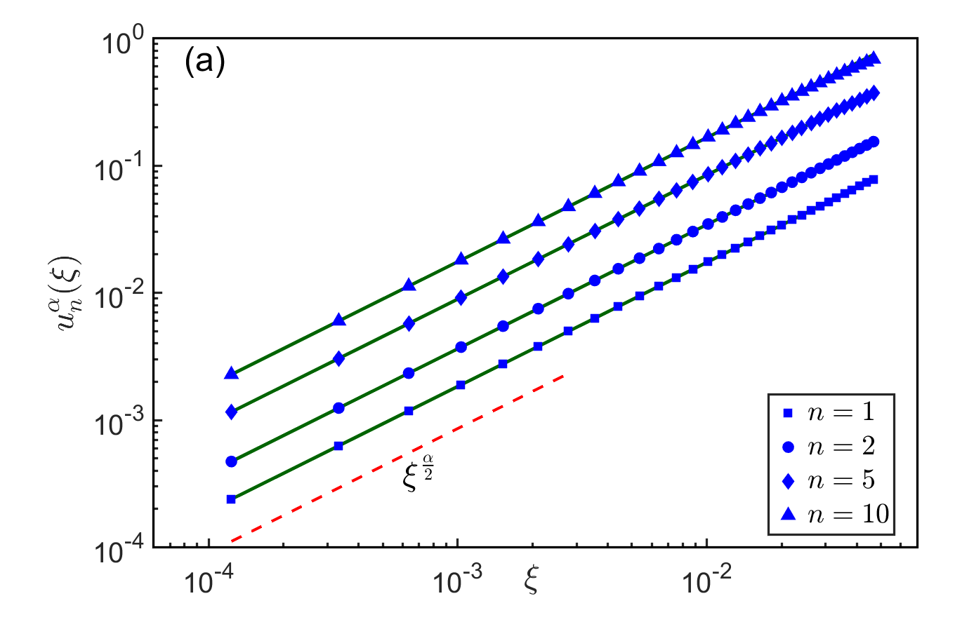
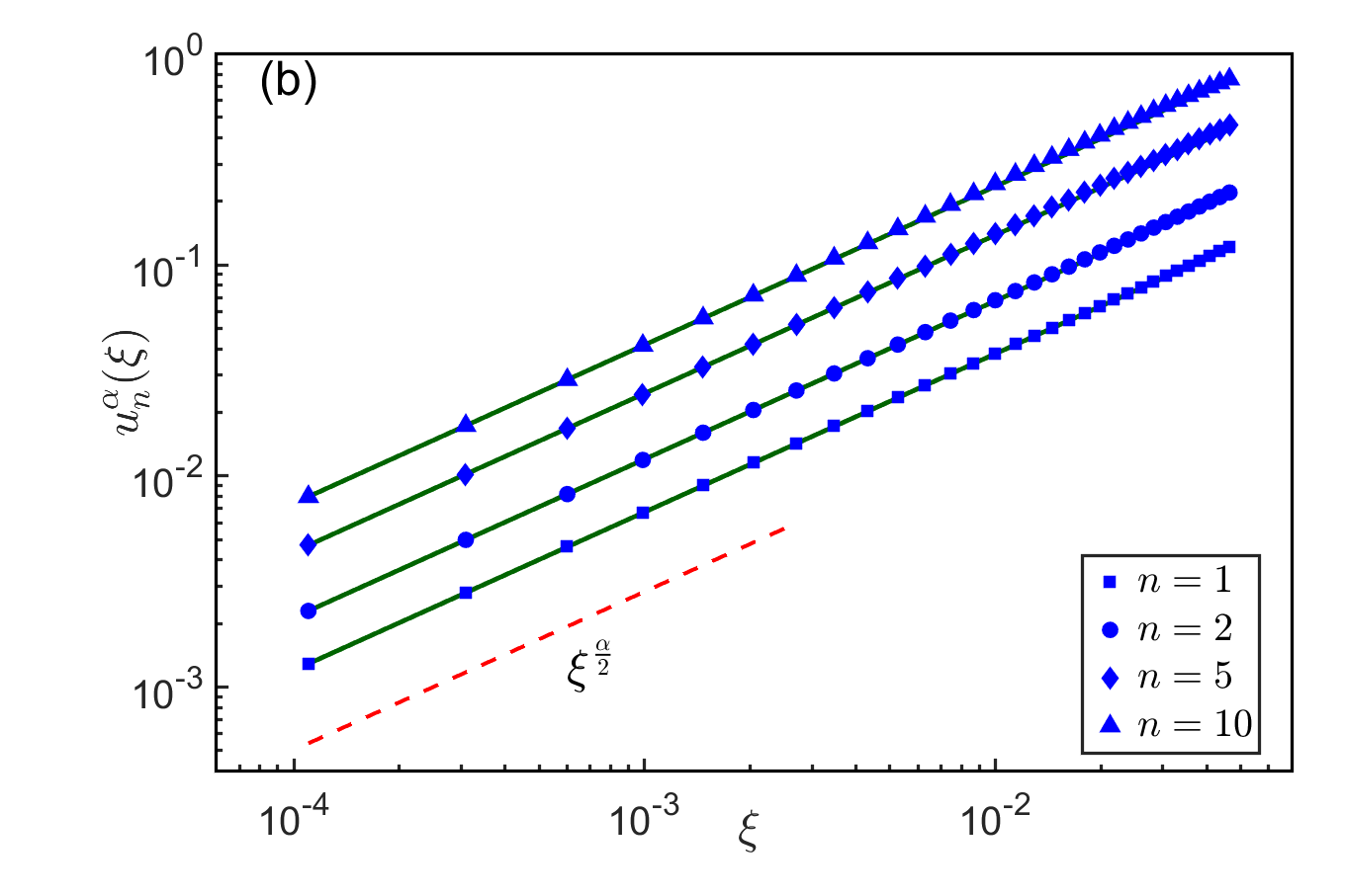
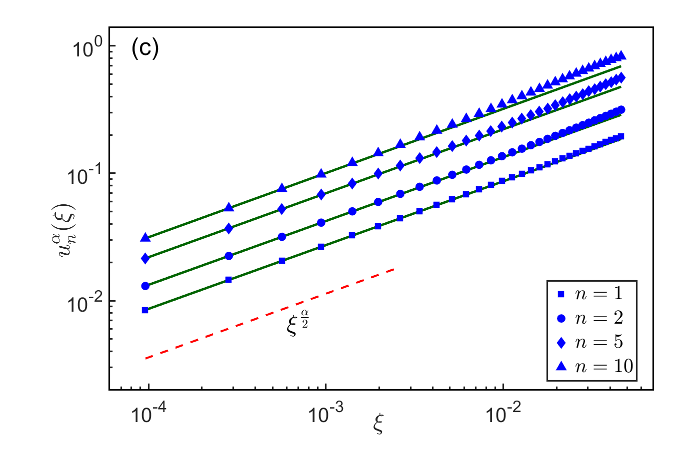
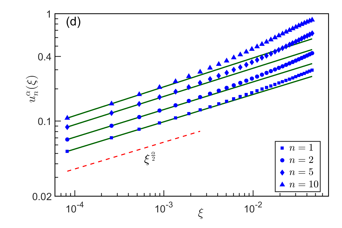
Figure 11: Singularity characteristics of different eigenfunctions of (1.1) with $\Omega=(-1,1)$, $V(x)\equiv 0$ and different $\alpha$ for (symbols denote numerical results and solids lines are from fitting formula $C\xi^{\alpha/2}$ when $0<\xi=x+1\ll 1$): (a) the first eigenfunction $u_{1}^{\alpha}$, (b) the second eigenfunction $u_{2}^{\alpha}$, (c) the fifth eigenfunction $u_{5}^{\alpha}$, and (d) the tenth eigenfunction $u_{10}^{\alpha}$.

From Figs. 9-11, we can draw the following conclusions: (i) Our JSM method (2.21) converges super-linearly with respect to the DOF $M$ for computing the eigenfunctions $u_{n}^{\alpha}$ (cf. Fig. 9). (ii) For fixed $0<\alpha<2$, the eigenfunctions $u_{n}^{\alpha}$ ($n=1,2,\ldots$) can be characterised as

$$u_{n}^{\alpha}(x)=(1-x^{2})^{\alpha/2}\,v_{n}^{\alpha}(x),\qquad-1\leq x\leq 1,$$ (4.11)

where $v_{n}^{\alpha}$ ($n=1,2,\ldots$) are smooth functions over the interval $\bar{\Omega}=[-1,1]$ (cf. Fig. 11). In addition, our numerical results indicate that, when $n\to\infty$ (cf. Fig. 10d), the eigenfunctions $u_{n}^{\alpha}$ ($0<\alpha<2$) of (1.1) with $\Omega=(-1,1)$ and $V(x)\equiv 0$ converge to the eigenfunction $u_{n}^{\alpha=2}=\sin(n\pi x)$ of (1.1) with $\alpha=2$, $\Omega=(-1,1)$ and $V(x)\equiv 0$, i.e.

$$u_{n}^{\alpha}(x)\to\sin\left(\frac{n\pi(x+1)}{2}\right)=u_{n}^{\alpha=2}(x),\qquad x\in\bar{\Omega},\qquad n\to\infty.$$ (4.12)

Based on the above results, for the eigenvalue problem of the FSO in high dimensions:

Find $\lambda\in\mathbb{R}$ and a nonzero real-valued function $u({\bf x})\neq 0$ such that

$$\begin{split}L_{\rm FSO}\;u({\bf x})&:=\left[(-\Delta)^{\alpha/2}+V({\bf x})\right]u({\bf x})=\lambda\;u({\bf x}),\qquad{\bf x}\in\Omega\subset{\mathbb{R}}^{d},\\ u({\bf x})&=0,\qquad{\bf x}\in\Omega^{c}:=\mathbb{R}^{d}\backslash\Omega,\end{split}$$ (4.13)

where $d\geq 2$, $0<\alpha<2$, $\Omega$ is a bounded domain and the fractional Laplacian $(-\Delta)^{\alpha/2}$ is defined via the Fourier transform [16, 47], we conjecture here that the eigenfunction $u({\bf x})$ can be written as

$$u({\bf x})=v({\bf x})\left({\rm dist}({\bf x},\partial\Omega)\right)^{\alpha/2},\qquad{\bf x}\in\bar{\Omega},$$ (4.14)

where $v({\bf x})$ is a smooth function over $\bar{\Omega}$ and ${\rm dist}({\bf x},\partial\Omega)$ represents the distance from ${\bf x}\in\Omega$ to $\partial\Omega$.

We remark here that the singularity characteristics of the eigenfunctions in (4.11) (or (4.14)) is quite different with the singularity characteristics given in [13] for fractional PDEs as

$$u({\bf x})\approx\left({\rm dist}({\bf x},\partial\Omega)\right)^{\alpha/2}+v({\bf x}),\qquad{\bf x}\in\bar{\Omega},$$ (4.15)

where $v({\bf x})$ is a smooth function over $\bar{\Omega}$. From our numerical results, we speculate that the correct singularity characteristics of the solution of fractional PDEs should be (4.14) instead of (4.15)!

5 Numerical results of FSO in 1D with potential

In this section, we report numerical results on eigenvalues of (1.1) with $\Omega=(-1,1)$ and $V(x)\neq 0$ by using our JSM (2.21) under the DOF $M=8192$. All results are based on the first $4096$ eigenvalues, i.e. we use half of the eigenvalues obtained numerically to present the results and to calculate distribution statistics. Here we consider four different external potentials given as:

Case I.   $V(x)=\frac{x^{2}}{2}$;

Case II.  $V(x)=4x^{2}$;

Case III. $V(x)=4x^{2}+\sin(\frac{\pi}{2}x)$;

Case IV. $V(x)=50x^{2}+\sin(2\pi x)$.

5.1 Eigenvalues and their asymptotics

	$\alpha=0.5$	$\alpha=1.0$	$\alpha=1.5$	$\alpha=1.9$	$\alpha=2.0$
$\lambda_{1}^{\alpha}$	1.0599238	1.240244372	1.6707307180	2.31063679348	2.53245197432
$\lambda_{2}^{\alpha}$	1.7684725	2.918074603	5.2120578091	8.73899699079	10.0106621605
$\lambda_{3}^{\alpha}$	2.1903345	4.481368142	9.7550085449	18.8734566366	22.3620761310
$\lambda_{4}^{\alpha}$	2.5518267	6.058660406	15.182580104	32.6230979973	39.6388288214
$\lambda_{5}^{\alpha}$	2.8580498	7.626501974	21.354271585	49.8832020720	61.8477048695
$\lambda_{6}^{\alpha}$	3.1370031	9.199495156	28.200700106	70.5802261928	88.9903414346
$\lambda_{7}^{\alpha}$	3.3893161	10.76885112	35.653816621	94.6494682651	121.067291745
$\lambda_{8}^{\alpha}$	3.6251388	12.34077821	43.673146060	122.040857583	158.078785000
$\lambda_{9}^{\alpha}$	3.8445549	13.91072820	52.217197374	152.708819987	200.024930128
$\lambda_{10}^{\alpha}$	4.0526430	15.48221913	61.258734930	186.615849002	246.905784303
$\lambda_{20}^{\alpha}$	5.5522311	31.02330310	174.43784577	697.513597025	986.960440109
$\lambda_{40}^{\alpha}$	7.8894197	62.43917340	495.71364899	2606.30876720	3947.84176043
$\lambda_{60}^{\alpha}$	9.6777480	93.85508927	912.11187382	5633.40862247	8882.64396098

Table 5: Different eigenvalues of (1.1) with $\Omega=(-1,1)$, $V(x)=\frac{x^{2}}{2}$ and different $\alpha$ obtained numerically by our JSM (2.21).

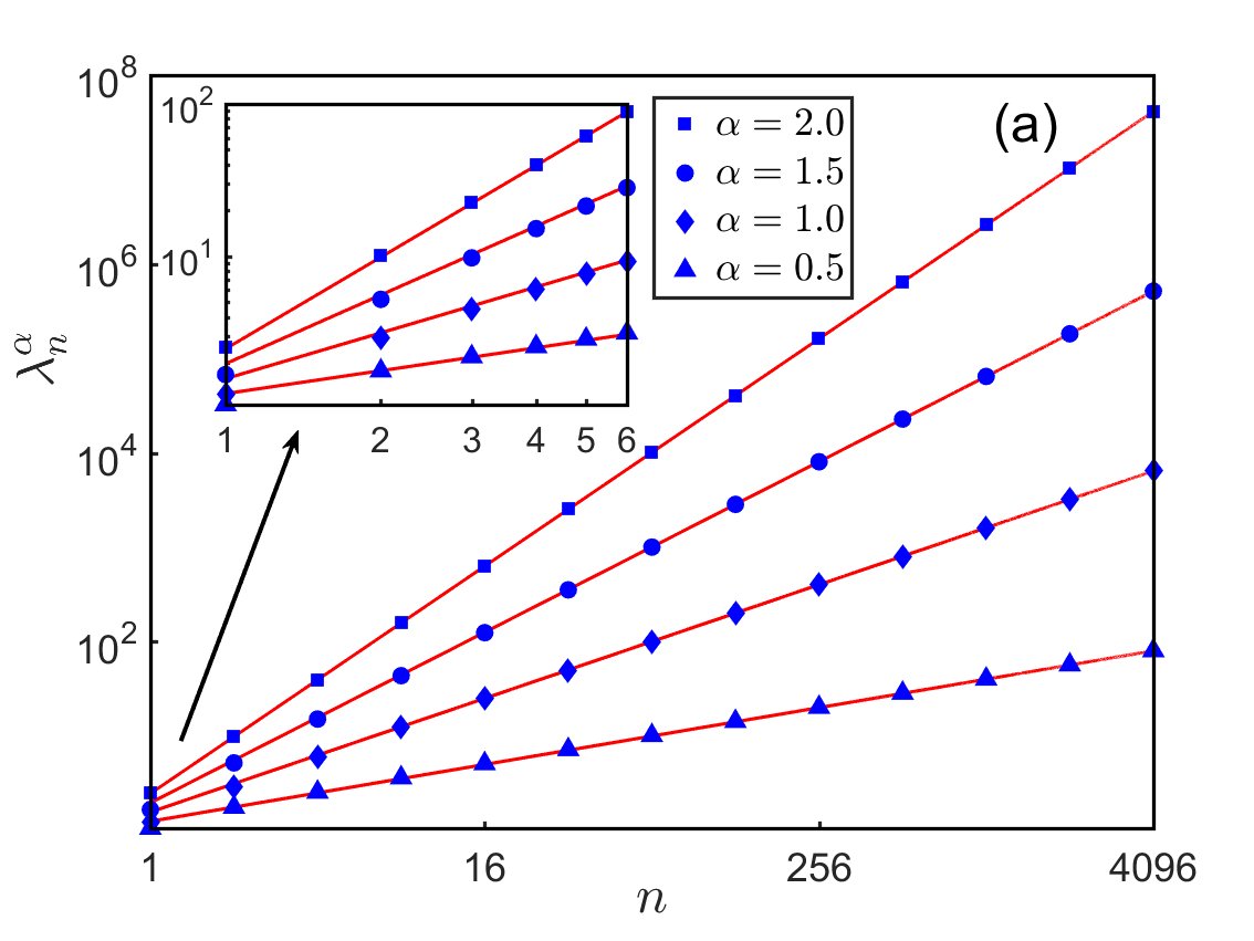
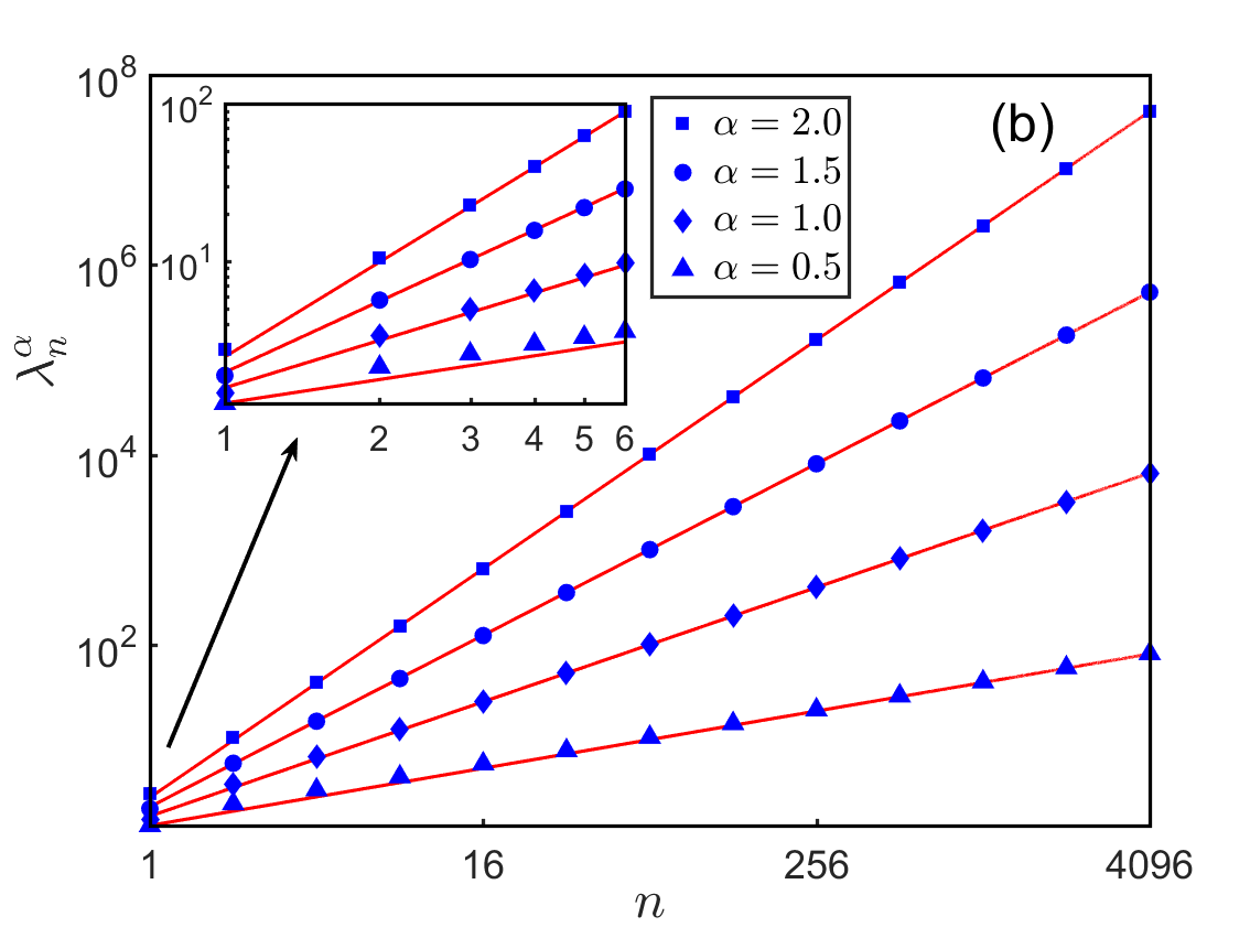
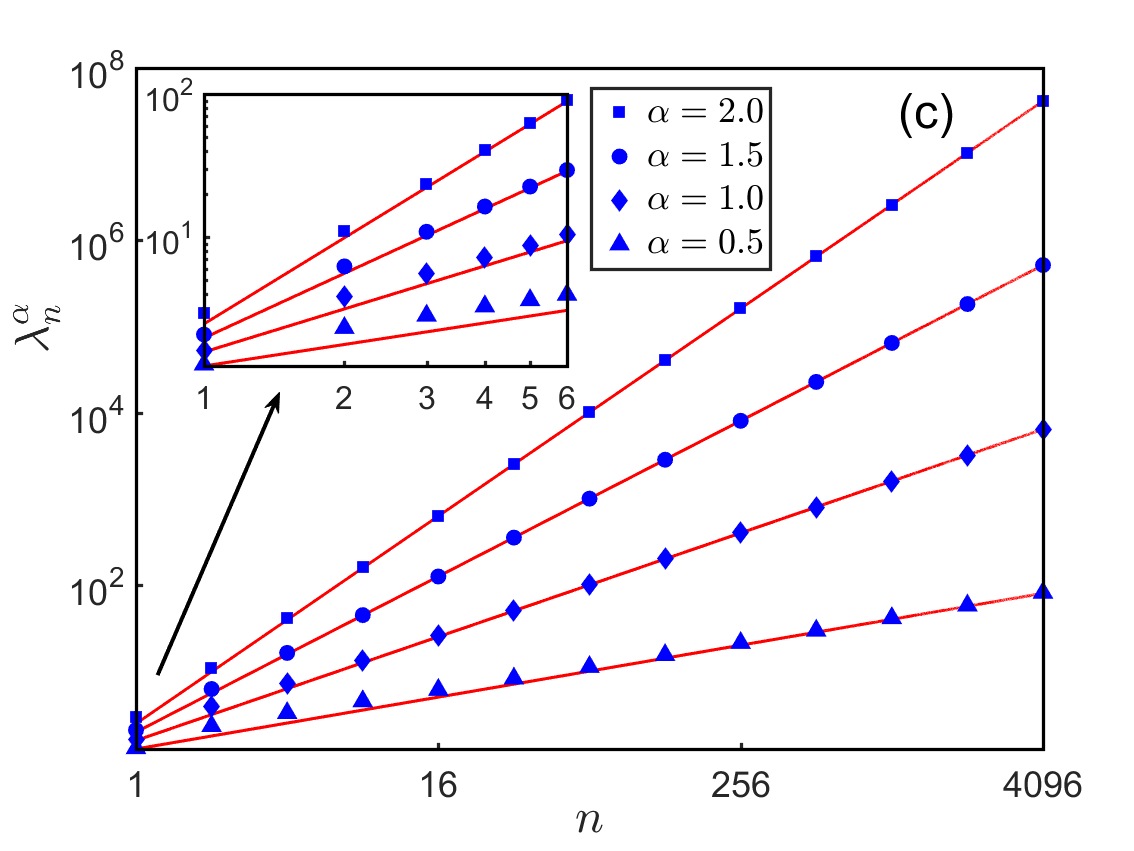
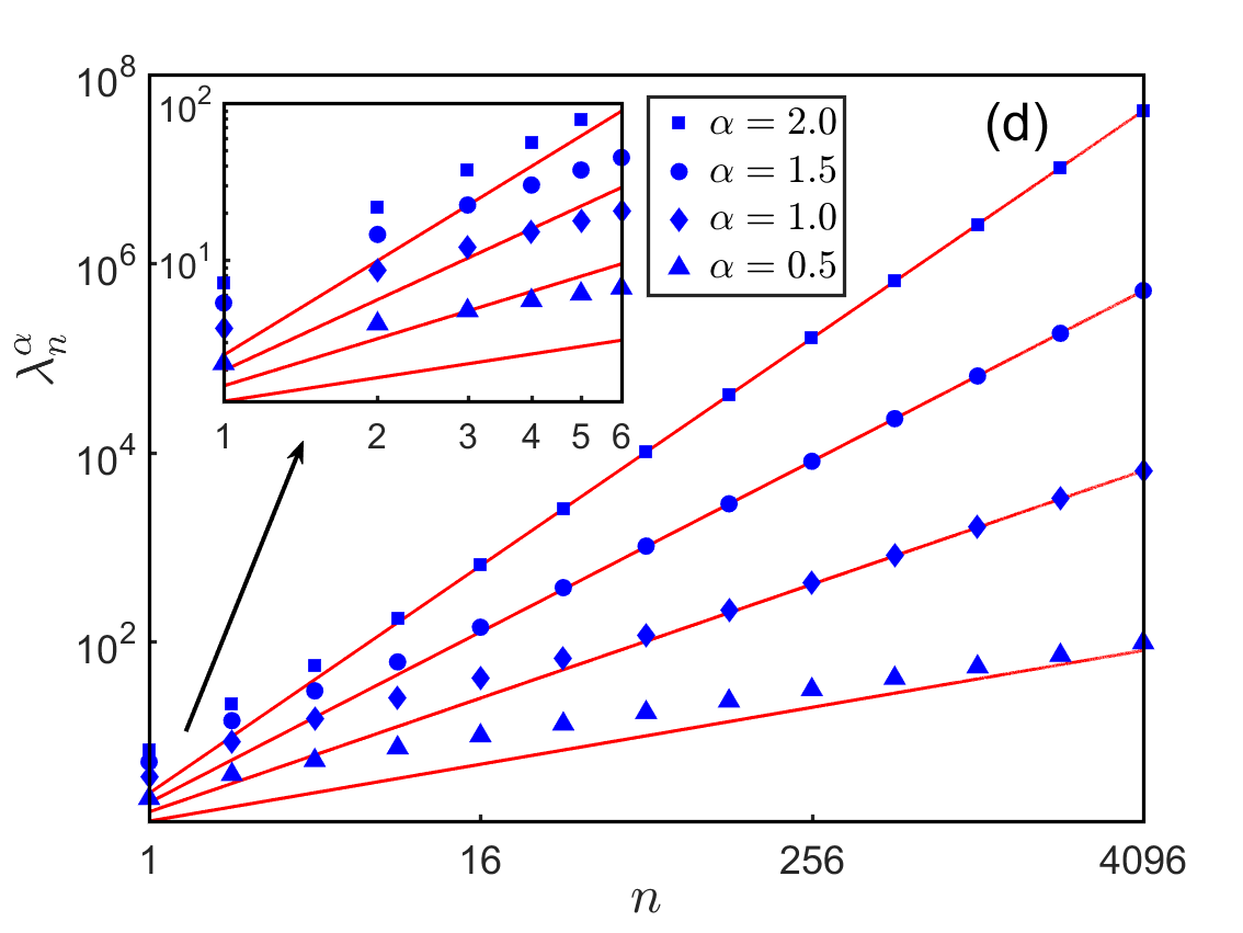
Figure 12: Eigenvalues $\lambda_{n}^{\alpha}$ ($n=1,2,\ldots,4096$) of (1.1) with $\Omega=(-1,1)$ and different $\alpha$ for differential external potentials (symbols denote numerical results and solids lines are from fitting formula when $n\gg 1$): (a) Case I, (b) Case II, (c) Case III, and (d) Case IV.

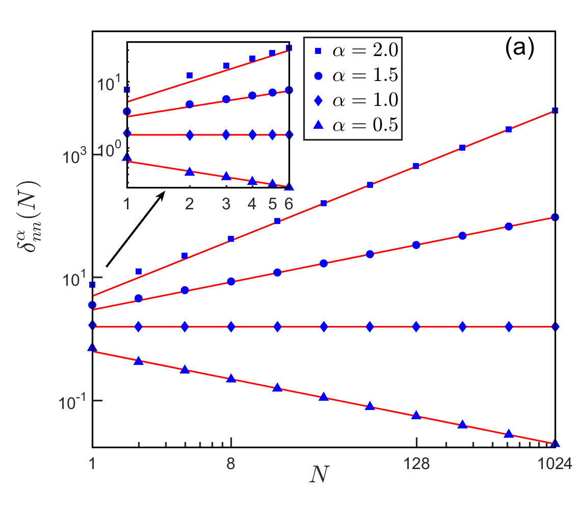
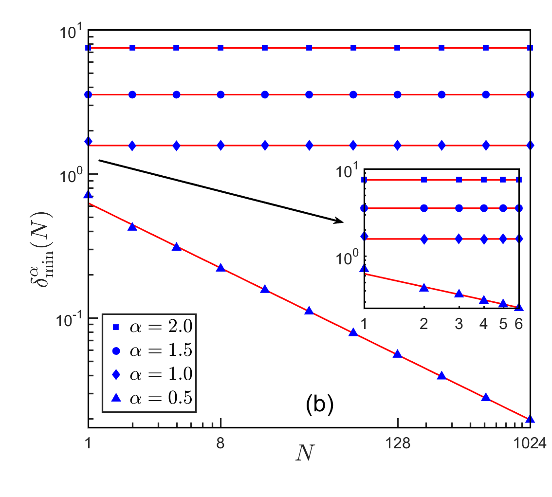
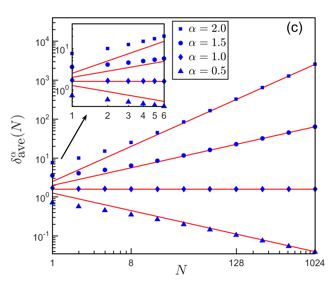
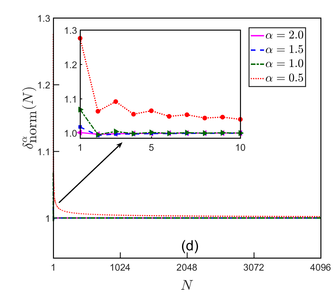
Figure 13: Different eigenvalue gaps of (1.1) with $\Omega=(-1,1)$, $V(x)=\frac{x^{2}}{2}$ and different $\alpha$ for (symbols denote numerical results and solids lines are from fitting formula when $N\gg 1$ in a-c): (a) the nearest neighbour gaps $\delta_{\rm nn}^{\alpha}(N)$, (b) the minimum gaps $\delta_{\textrm{min}}^{\alpha}(N)$, (c) the average gaps $\delta_{\textrm{ave}}^{\alpha}(N)$, and (d) the normalized gaps $\delta_{\textrm{norm}}^{\alpha}(N)$.

Table 5 lists the eigenvalues of (1.1) with $\Omega=(-1,1)$ and $V(x)=\frac{x^{2}}{2}$ for different $\alpha$. Figure 12 plots the eigenvalues of (1.1) with $\Omega=(-1,1)$, different external potentials $V(x)$ and different $\alpha$.

From Fig. 12, we can conclude that, when $n\gg 1$, the leading order asymptotics of the eigenvalues $\lambda_{n}^{\alpha}$ in (4.1) is still valid for the eigenvalue problem of FSO (1.1) with potential $V(x)$.

5.2 Gaps and their distribution statistics

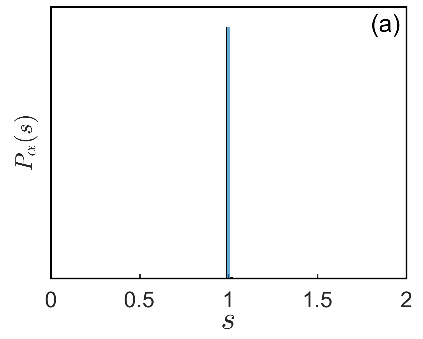
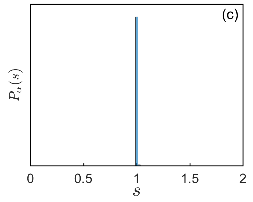
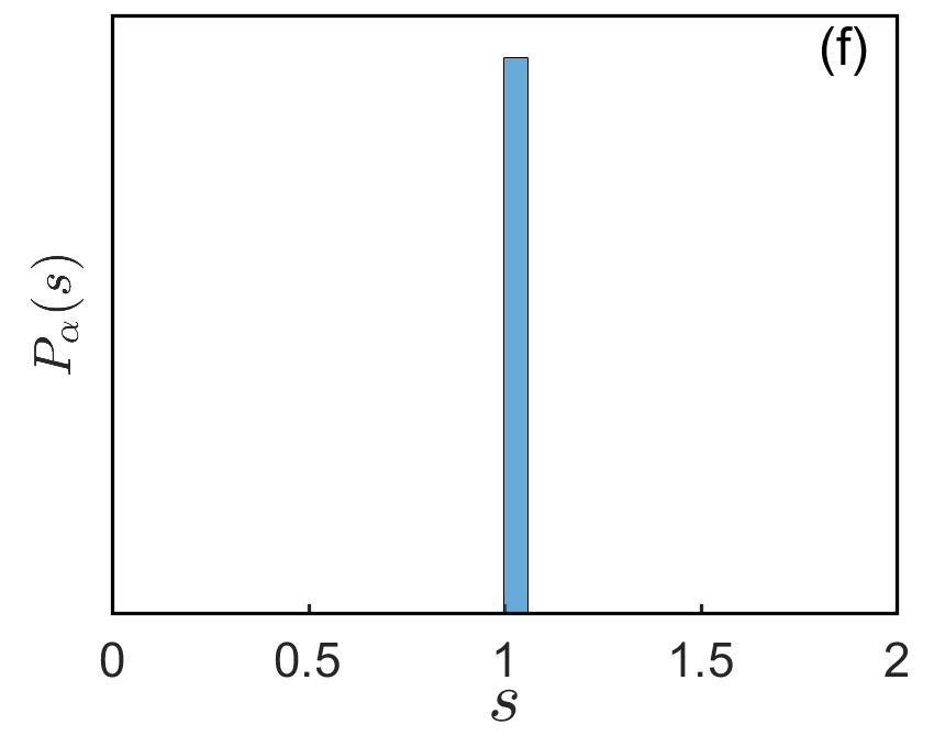
Figure 14: The histogram of the normalized gaps $\{\delta_{\rm norm}^{\alpha}(n)\ |\ 1\leq n\leq N=4096\}$ of (1.1) with $\Omega=(-1,1)$ and $V(x)=\frac{x^{2}}{2}$ for different $\alpha$: (a) $\alpha=2.0$, (b) $\alpha=1.9$, (c) $\alpha=\sqrt{3}$, (d) $\alpha=1.5$, (e) $\alpha=1.0$, and (f) $\alpha=0.5$.

Figure 13 plots different eigenvalue gaps of (1.1) with $\Omega=(-1,1)$, $V(x)=\frac{x^{2}}{2}$ and different $\alpha$. Figure 14 displays the histogram of the normalized gaps $\{\delta_{\rm norm}^{\alpha}(n)\ |\ 1\leq n\leq N=4096\}$ defined in (4.9) for (1.1) with $\Omega=(-1,1)$, $V(x)=\frac{x^{2}}{2}$ and different $\alpha$. For other potentials, our numerical results show similar behavior on eigenvalues and their gaps, which are omitted here for brevity.

Again, from Figs. 13 and 14, we can conclude that, when $n\gg 1$, the asymptotics of the eigenvalue gaps given in (4.3), (4.4), (4.6), (4.7), (4.8) and (4.9) are still valid for the eigenvalue problem of FSO (1.1) with potential $V(x)$. In addition, the gaps distribution statistics is still $P_{\alpha}(s)=\delta(s-1)$ for $0<\alpha\leq 2$ in this case.

5.3 Comparison on eigenvalues of (1.1) without and with potential

Let $0<\lambda_{1}^{\alpha,0}<\lambda_{2}^{\alpha,0}<\ldots<\lambda_{n}^{\alpha,0}<\ldots$ be all eigenvalues of (1.1) with $\Omega=(-1,1)$ and $V(x)\equiv 0$, and denote all eigenvalues of (1.1) with a potential $V$ as in (1.4). Figure 15 plots differences of the eigenvalues of (1.1) with a potential $V$ and without a potential, i.e. $\delta_{n}^{V}:=\lambda_{n}^{\alpha}-\lambda_{n}^{\alpha,0}-C_{V}$ ($1\leq n\leq N=4096$) for different potentials $V(x)$ and $\alpha$, where $C_{V}=\frac{1}{2}\int_{-1}^{1}V(x)dx$.

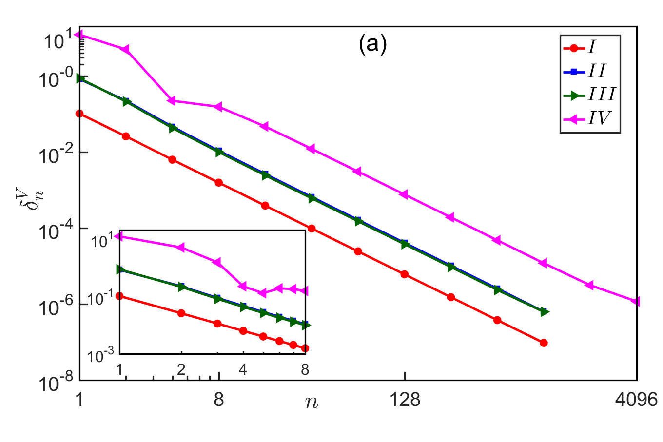
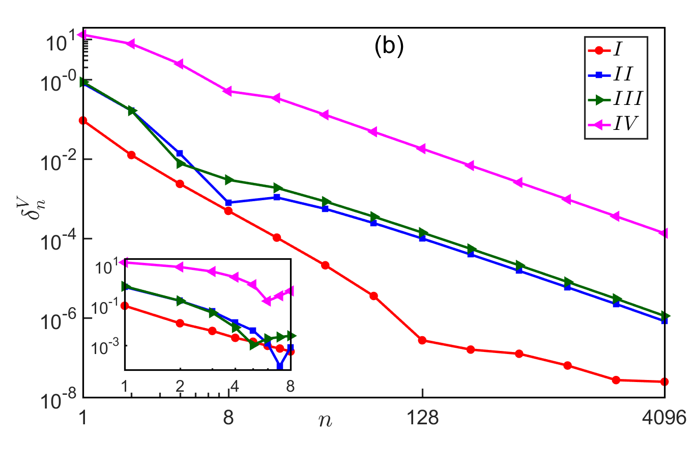
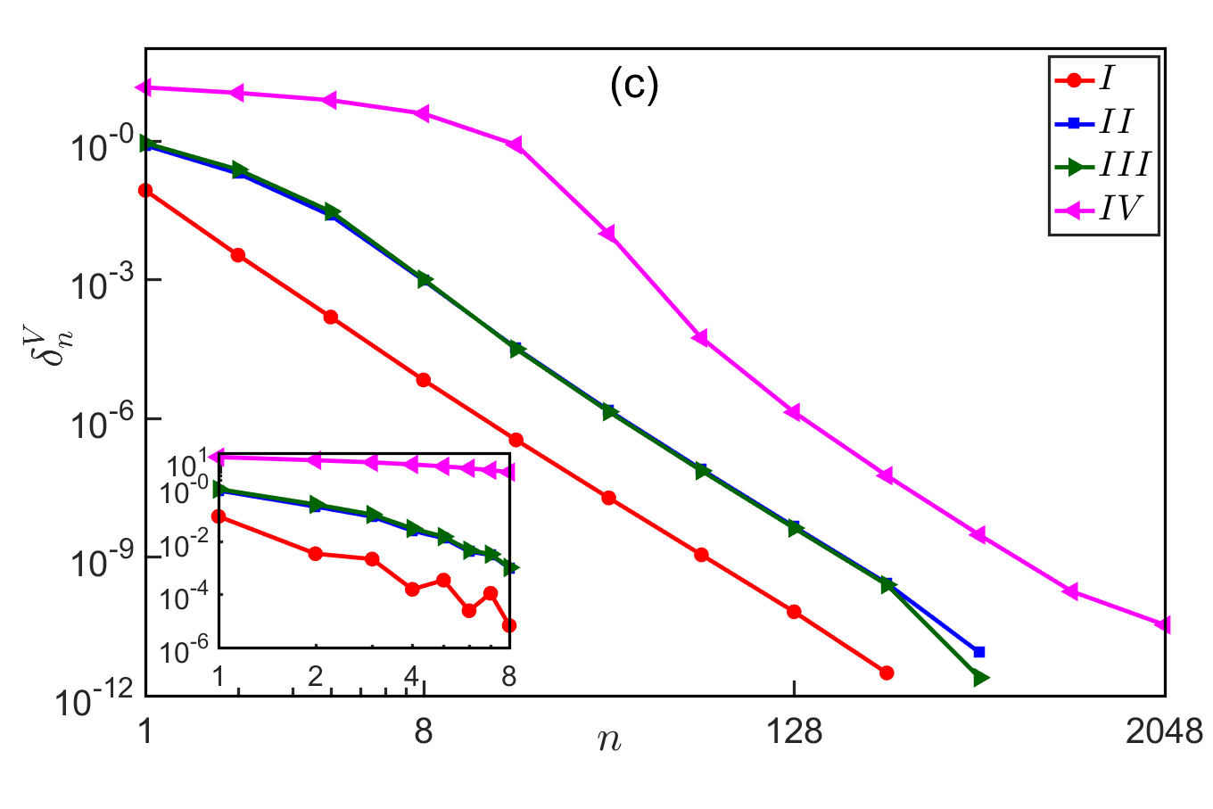
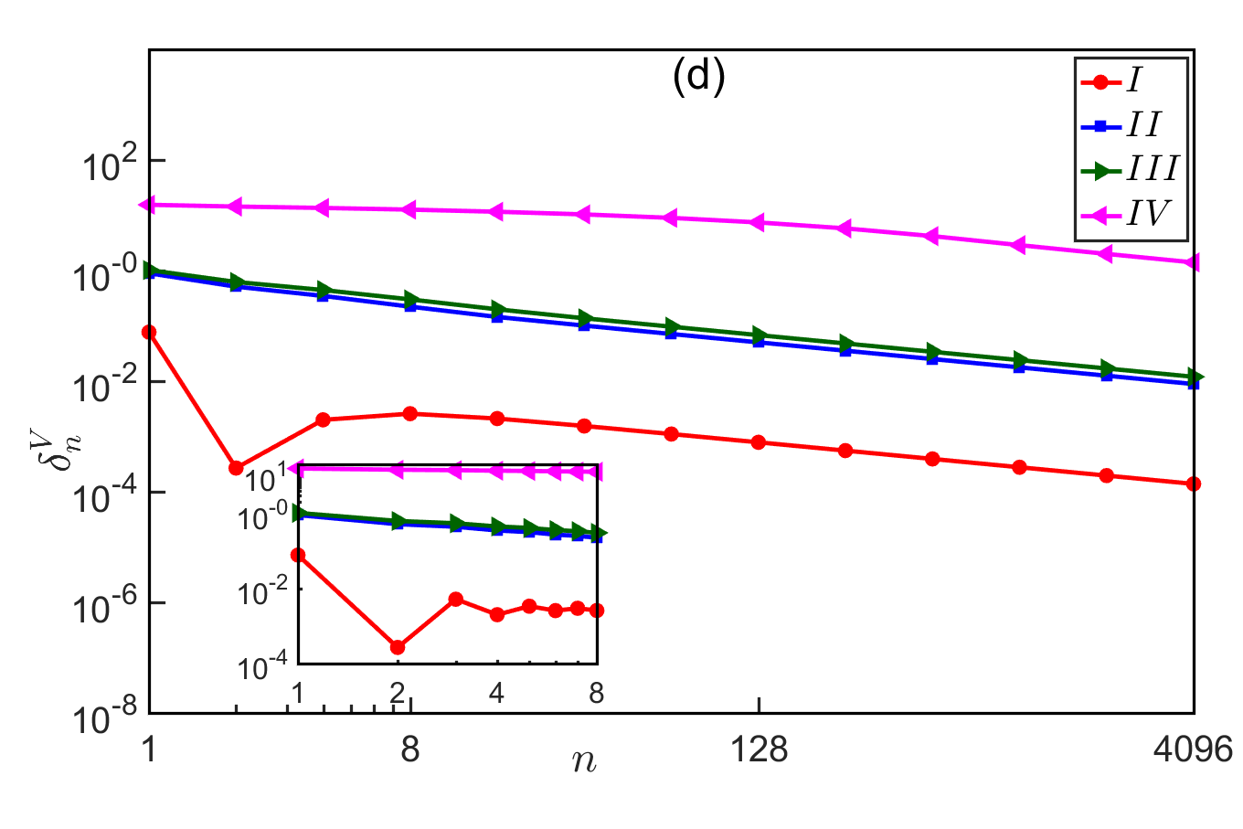
Figure 15: Differences of the eigenvalues of (1.1) with a potential $V$ and without a potential, i.e. $\delta_{n}^{V}:=\lambda_{n}^{\alpha}-\lambda_{n}^{\alpha,0}-C_{V}$ ($1\leq n\leq N=4096$) for different potentials $V(x)$ and $\alpha$: (a) $\alpha=2$, (b) $\alpha=\sqrt{2}$, (c) $\alpha=1$, and (d) $\alpha=0.5$.

From Fig. 15, we can draw the following conclusion for the eigenvalues of (1.1) with a potential $V$:

$$\lambda_{n}^{\alpha}=\lambda_{n}^{\alpha,0}+C_{V}+O\left(n^{-\tau_{1}(\alpha)}\right),\qquad n\gg 1,$$ (5.1)

where

$$\tau_{1}(\alpha)=\left\{\begin{array}[]{ll}\alpha&0<\alpha\leq 2\&\alpha\neq 1,\\ \approx 4.5&\alpha=1,\\ \end{array}\right.$$ (5.2)

5.4 Eigenfunctions

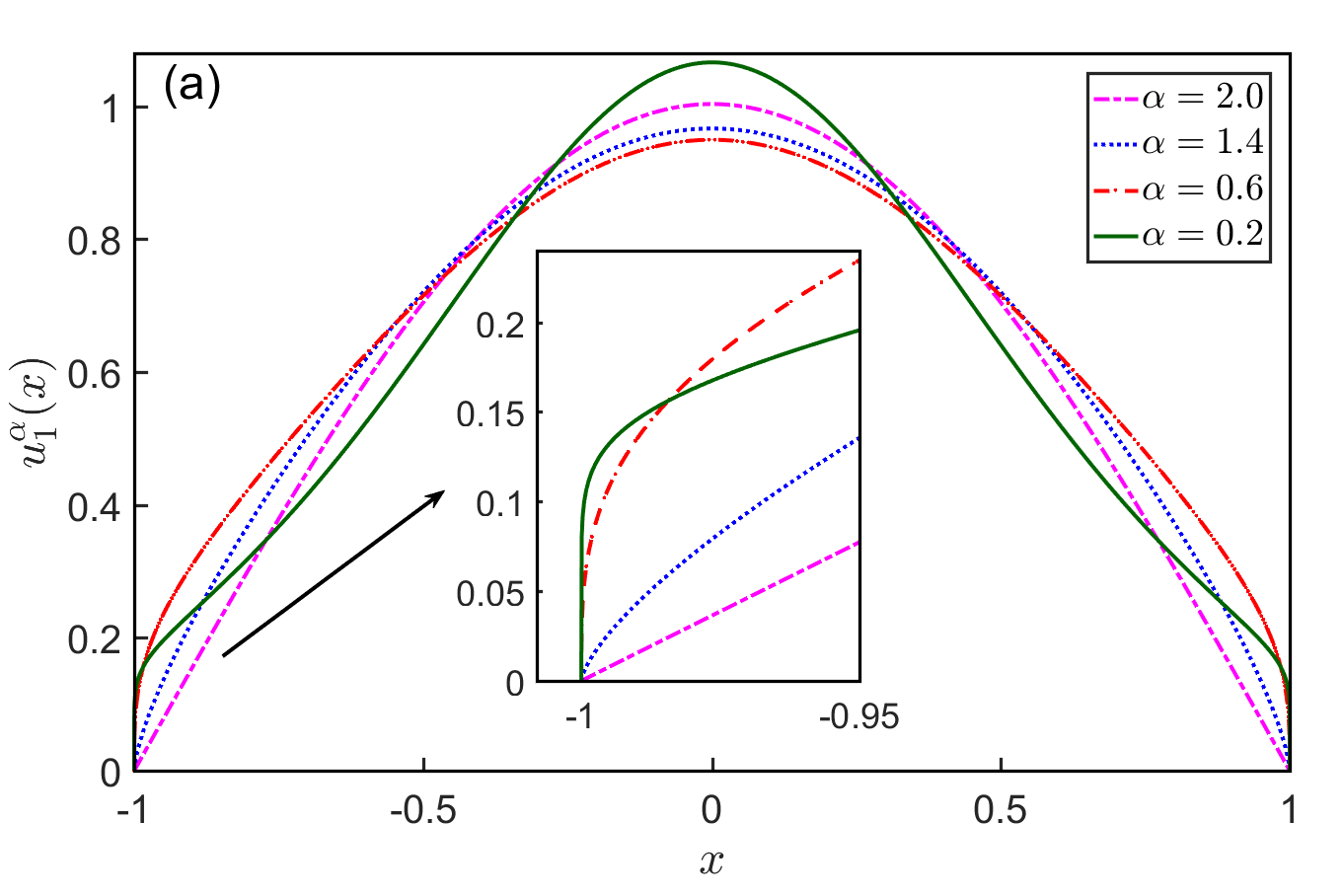
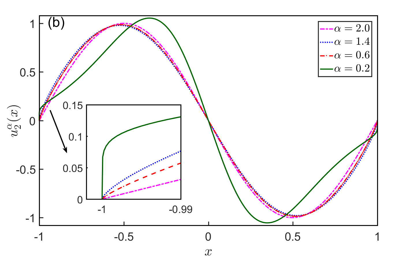
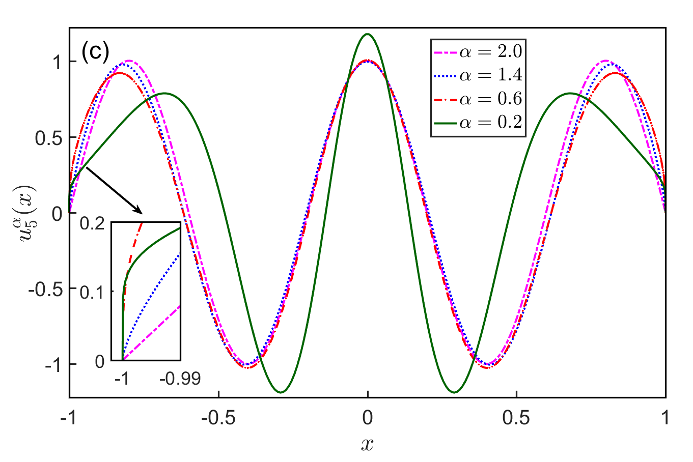
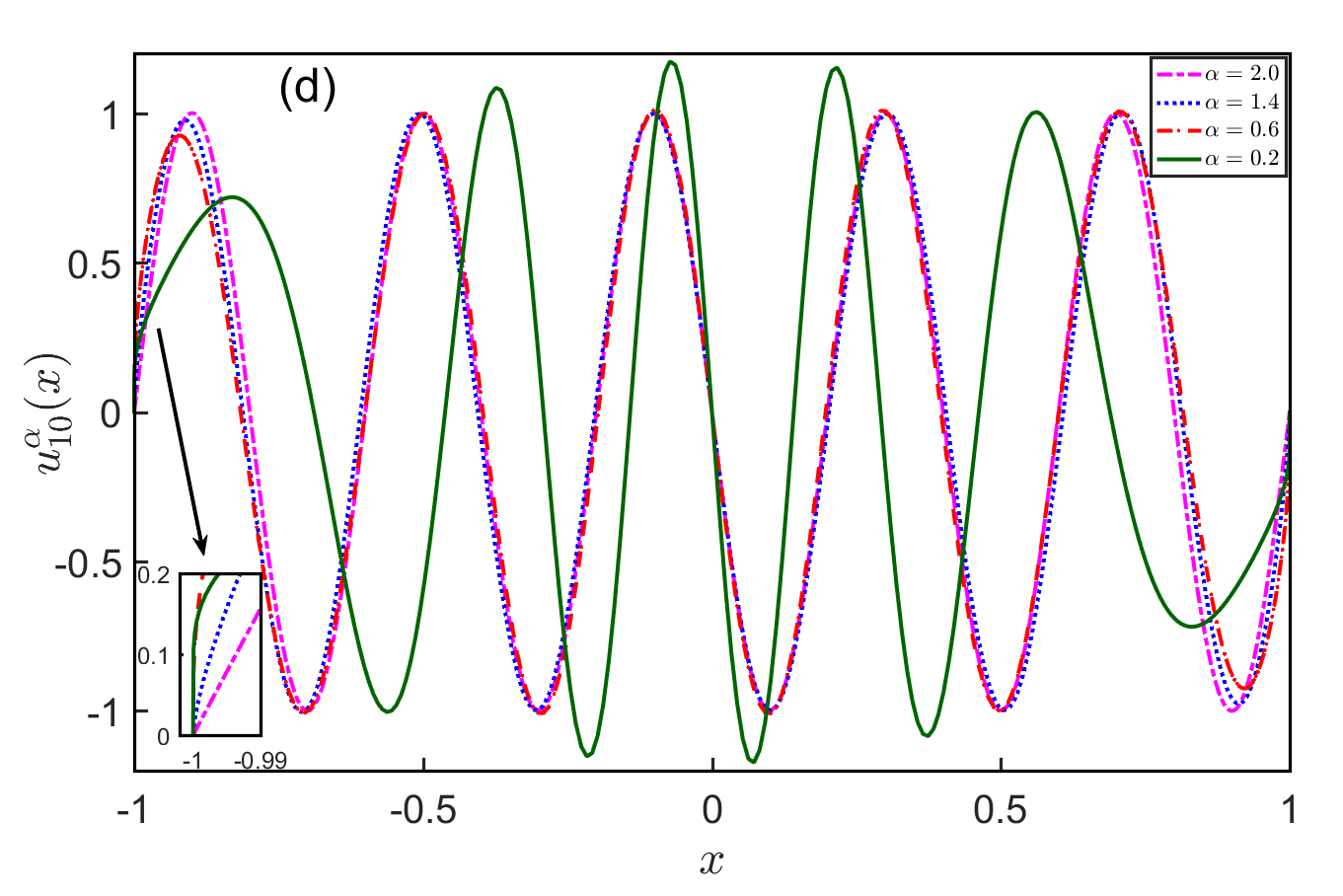
Figure 16: Plots of different eigenfunctions of (1.1) with $\Omega=(-1,1)$, $V(x)=\frac{x^{2}}{2}$ and different $\alpha$: (a) the first eigenfunction $u_{1}^{\alpha}(x)$, (b) the second eigenfunction $u_{2}^{\alpha}(x)$, (c) the fifth eigenfunction $u_{5}^{\alpha}(x)$, and (d) the tenth eigenfunction $u_{10}^{\alpha}(x)$.

Figure 16 plots different eigenfunctions $u_{n}^{\alpha}$ of (1.1) with $\Omega=(-1,1)$ and $V(x)=\frac{x^{2}}{2}$ for different $\alpha$.

From Fig. 16, the singularity characteristics of the eigenfunction given in (4.11) is still valid for the eigenvalue problem of FSO (1.1) with potential $V(x)$. In addition, our numerical results indicate that, when $n\to\infty$ (cf. Fig. 10d), the eigenfunctions $u_{n}^{\alpha}$ ($0<\alpha<2$) of (1.1) with a potential $V$ converge to the eigenfunction $u_{n}^{\alpha=2}=\sin\left(\frac{n\pi(x+1)}{2}\right)$ which is the eigenfunction of (1.1) with $\alpha=2$ and $V(x)\equiv 0$.

Finally, based on our extensive numerical results and observations, we speculate the following observation (or conjecture) for the FSO in (1.1) with potential:

Conjecture II (Gaps and their distribution statistics of FSO in (1.1) with potential) Assume $1<\alpha\leq 2$ and $V(x)\in C(\bar{\Omega})$ in (1.1), then we have the following asymptotics of its eigenvalues:

$$\lambda_{n}^{\alpha}=\left\{\begin{array}[]{ll}\left(\frac{n\pi}{b-a}\right)^{\alpha}-\left(\frac{\pi}{b-a}\right)^{\alpha}\frac{\alpha(2-\alpha)}{4}n^{\alpha-1}+C_{V}+O(n^{\alpha-2}),&1<\alpha\leq 2,\\ \frac{n\pi}{b-a}-\frac{\pi}{4(b-a)}+C_{V}+O(n^{-1}),&\alpha=1,\\ \left(\frac{n\pi}{b-a}\right)^{\alpha}+C_{V}-\left(\frac{\pi}{b-a}\right)^{\alpha}\frac{\alpha(2-\alpha)}{4}n^{\alpha-1}+O(n^{-\alpha}),&0<\alpha<1,\\ \end{array}\right.\qquad n\gg 1,$$ (5.3)

where

$$C_{V}=\frac{1}{|\Omega|}\int_{\Omega}V(x)dx=\frac{1}{b-a}\int_{a}^{b}V(x)dx.$$ (5.4)

In addition, we have the following asymptotics for different gaps:

$$\begin{split}&\delta_{\rm nn}^{\alpha}(N)\approx\left(\frac{\pi}{b-a}\right)^{\alpha}\left[\alpha N^{\alpha-1}+\frac{\alpha(\alpha-1)(2+\alpha)}{4}N^{\alpha-2}+O(N^{\alpha-3})\right],\qquad 0<\alpha\leq 2,\\ &\delta_{\rm min}^{\alpha}(N)=\lambda_{N+1}^{\alpha}-\lambda_{N}^{\alpha}\approx\alpha\left(\frac{\pi}{b-a}\right)^{\alpha}N^{\alpha-1},\qquad 0<\alpha<1,\\ &\delta_{\rm ave}^{\alpha}(N)\approx\left(\frac{\pi}{b-a}\right)^{\alpha}\left\{\begin{array}[]{ll}\vspace{2mm}\left[N^{\alpha-1}+\frac{\alpha(2+\alpha)}{4}N^{\alpha-2}+O(N^{-1})\right],&1<\alpha\leq 2,\\ \vspace{2mm}\left[1+\left(\frac{3}{4}-\frac{b-a}{\pi}\lambda_{1}^{\alpha=1}\right)N^{-1}+O(N^{-2})\right],&\alpha=1,\\ \left[N^{\alpha-1}-\left(\frac{b-a}{\pi}\right)^{\alpha}\lambda_{1}^{\alpha}N^{-1}+O(N^{\alpha-2})\right],&0<\alpha<1,\\ \end{array}\right.\\ &\delta_{\rm norm}^{\alpha}(N)\approx 1+O(N^{-2}),\qquad 0<\alpha\leq 2,\end{split}\qquad N\gg 1.$$ (5.5)

In addition, for the gaps distribution statistics defined in (1.11), we have

$$P_{\alpha}(s)=\delta(s-1),\qquad s\geq 0,\qquad 0<\alpha\leq 2.$$ (5.6)

6 Extension to directional fractional Schrödinger operator in high dimensions

In this section, we extend the Jacobi spectral method (JSM) presented in Section 2 to directional fractional Schrödinger operator (D-FSO) in high dimensions and apply it to study numerically its eigenvalues and their gaps as well as gap distribution statistics.

6.1 D-FSO in high dimensions

Consider the eigenvalue problem related to the directional fractional Schrödinger operator (D-FSO) in high dimensions:

Find $\lambda\in\mathbb{R}$ and a nonzero real-valued function $u({\bf x})\neq 0$ such that

$$\begin{split}L_{\hbox{D-FSO}}\;u({\bf x})&:=\left[\mathcal{D}^{\alpha}_{\mathbf{x}}+V({\bf x})\right]u({\bf x})=\lambda\;u({\bf x}),\qquad{\bf x}\in\Omega:=(-L_{1},L_{1})\times\ldots(-L_{d},L_{d})\subset{\mathbb{R}}^{d},\\ u({\bf x})&=0,\qquad{\bf x}\in\Omega^{c}:=\mathbb{R}^{d}\backslash\Omega,\end{split}$$ (6.1)

where $d\geq 2$, ${\bf x}=(x_{1},x_{2},\ldots,x_{d})^{T}$, $0<\alpha\leq 2$, $V({\bf x})\in L^{2}(\Omega)$ is a given real-valued function and the directional fractional Laplacian operator $\mathcal{D}^{\alpha}_{\mathbf{x}}:=\sum_{j=1}^{d}(-\partial_{x_{j}x_{j}})^{\alpha/2}$ is defined via the Fourier transform (see [16, 47, 40] and references therein) as

$$\mathcal{D}^{\alpha}_{\mathbf{x}}\;u({\bf x})={\mathcal{F}}^{-1}\left(\sum_{j=1}^{d}|\xi_{j}|^{\alpha}(\mathcal{F}u)(\boldsymbol{\xi})\right)\qquad{\bf x},\boldsymbol{\xi}\in\mathbb{R}^{d},$$ (6.2)

with $\boldsymbol{\xi}=(\xi_{1},\xi_{2},\ldots,\xi_{d})^{T}$, ${\mathcal{F}}$ and ${\mathcal{F}}^{-1}$ the Fourier transform and inverse Fourier transform over ${\mathbb{R}}^{d}$ [51, 57], respectively. We remark here that the directional fractional Laplacian operator $\mathcal{D}^{\alpha}_{\mathbf{x}}$ has been widely used in the literature for different fractional PDEs, see [41, 61, 45, 29, 40] and references therein. Without loss of generality, we assume that $L_{1}\geq L_{2}\geq\ldots\geq L_{d}>0$.

Again, since all eigenvalues of (6.1) are distinct (or all spectrum are discrete and no continuous spectrum), similar to (1.4) for (1.1), we can also rank (or order) all eigenvalues of (6.1) as (1.4), while again the times that an eigenvalue $\lambda$ of (6.1) appears in the sequence (1.4) is the same as its algebraic multiplicity. Under the order of all eigenvalues in (1.4) for (6.1), we define the fraction of repeated eigenvalues of (6.1) as

$$R^{\alpha}(N):=\frac{\#\{2\leq n\leq N\ |\ \lambda_{n}^{\alpha}=\lambda_{n-1}^{\alpha}\}}{N},\qquad N=2,3,\ldots\;.$$ (6.3)

In addition, let $0<\lambda_{1}^{\alpha,0}<\lambda_{2}^{\alpha,0}<\ldots<\lambda_{n}^{\alpha,0}<\ldots$ be all eigenvalues of (1.1) with $\Omega=(-1,1)$ and $V(x)\equiv 0$, and $u_{n}^{\alpha,0}(x)$ ($n=1,2,\ldots$) be the corresponding eigenfunctions. Then when $V({\bf x})\equiv 0$ in (6.1), all eigenvalues of the problem (6.1) can be given as

$$\lambda_{j_{1}\ldots j_{d}}^{\alpha}=\sum_{l=1}^{d}L_{l}^{-\alpha}\lambda_{j_{l}}^{\alpha,0},\qquad j_{1},\ldots,j_{d}=1,2,\ldots,$$ (6.4)

and their corresponding eigenfunctions can be given as

$$u_{j_{1}\ldots j_{d}}^{\alpha}({\bf x})=\Pi_{l=1}^{d}u_{j_{l}}^{\alpha,0}(x_{l}/L_{l}),\qquad{\bf x}\in\bar{\Omega},\qquad j_{1},\ldots,j_{d}=1,2,\ldots\;.$$ (6.5)

The above results immediately imply that the fundamental gap of (6.1) with $V({\bf x})\equiv 0$ can be obtained as

$$\delta_{\rm fg}(\alpha)=L_{1}^{-\alpha}\lambda_{2}^{\alpha,0}+\sum_{l=2}^{d}L_{l}^{-\alpha}\lambda_{1}^{\alpha,0}-\sum_{l=1}^{d}L_{l}^{-\alpha}\lambda_{1}^{\alpha,0}=L_{1}^{-\alpha}\left(\lambda_{2}^{\alpha,0}-\lambda_{1}^{\alpha,0}\right)\geq\frac{\lambda_{2}^{\alpha,0}-\lambda_{1}^{\alpha,0}}{(D/2)^{\alpha}},$$ (6.6)

where $D$ is the diameter of $\Omega$.

The JSM presented in Section 2 can be easily extended to solve the eigenvalue problem (6.1) by tensor product [45]. The details are omitted here for brevity.

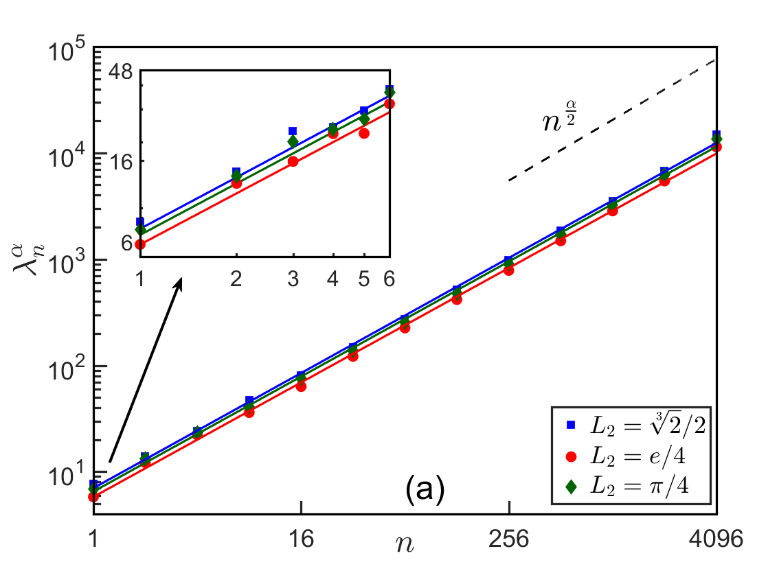
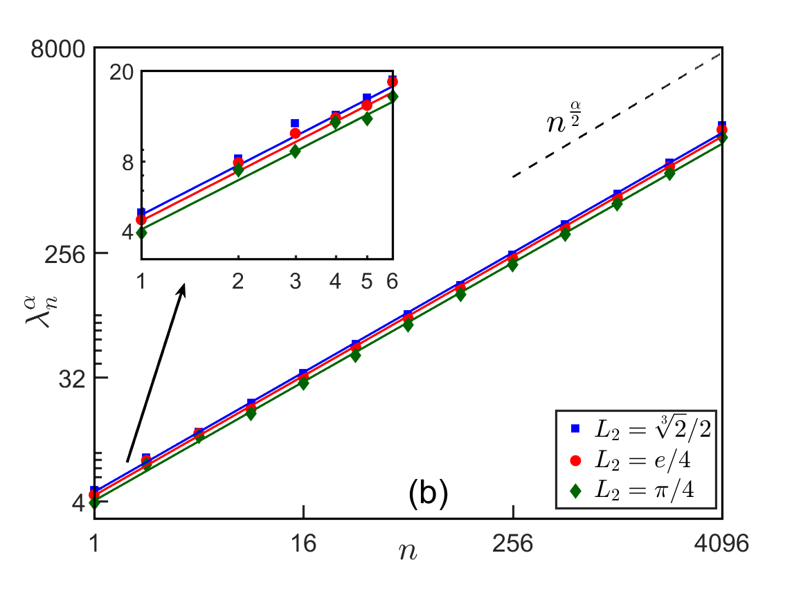
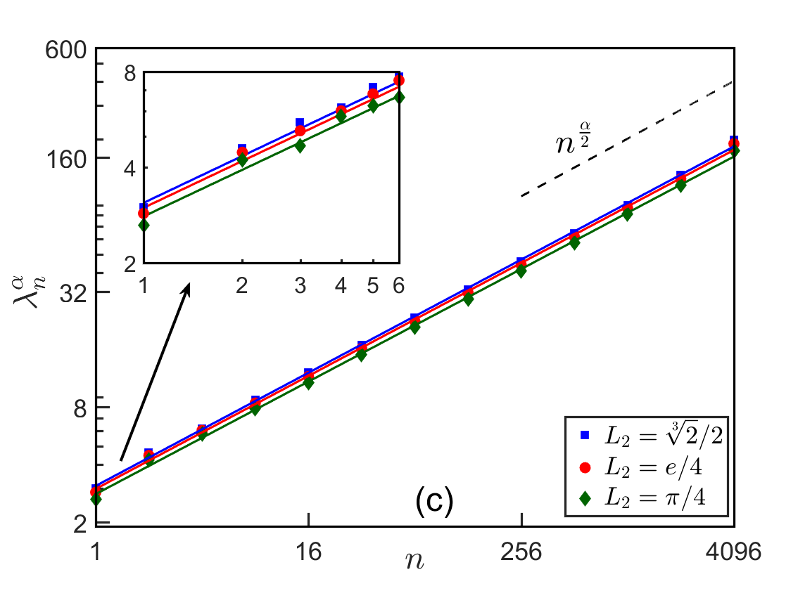
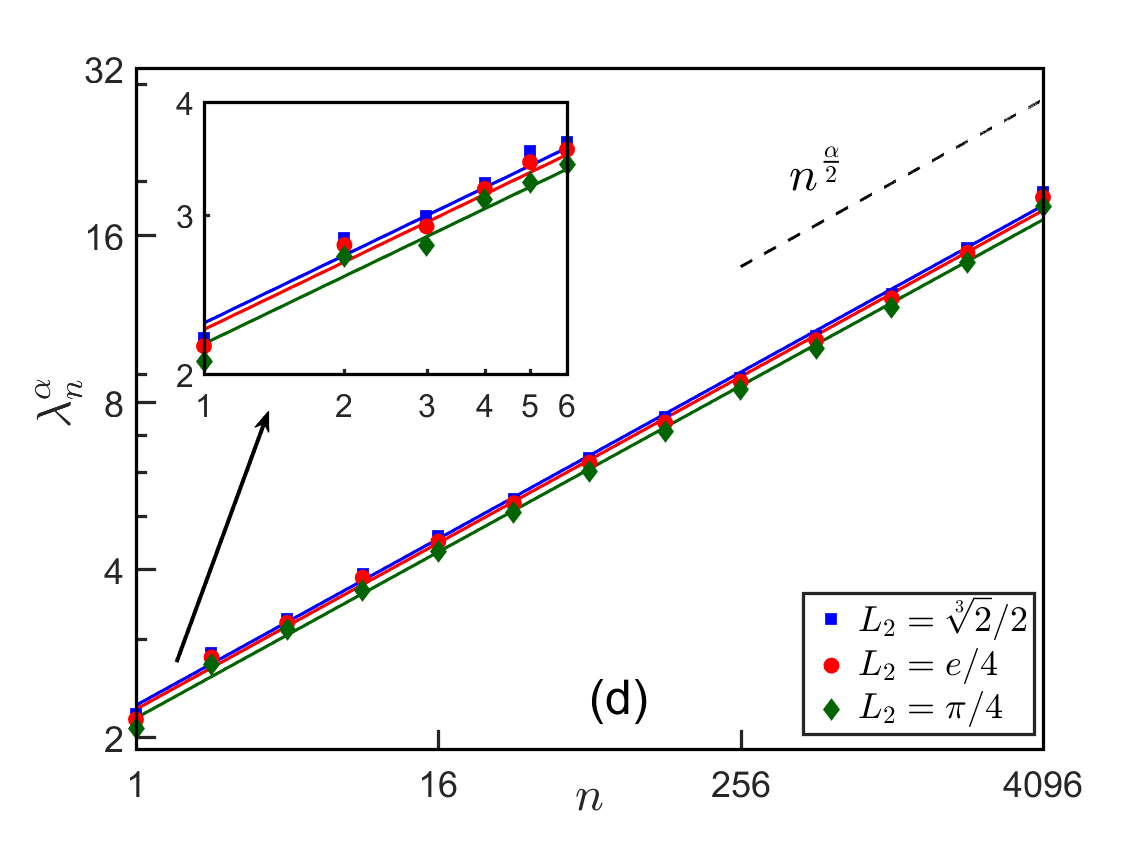
Figure 17: Eigenvalues of (6.1) with $d=2$, $L_{1}=1$, $V({\bf x})\equiv 0$ and different $L_{2}$ and $\alpha$ (symbols denote numerical results and solids lines are from fitting formula $C_{2}^{\alpha}n^{\alpha/2}$ when $n\gg 1$): (a) $\alpha=1.9$, (b) $\alpha=1.5$, (c) $\alpha=1.0$, and (d) $\alpha=0.5$.

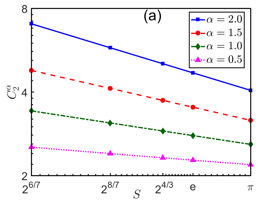
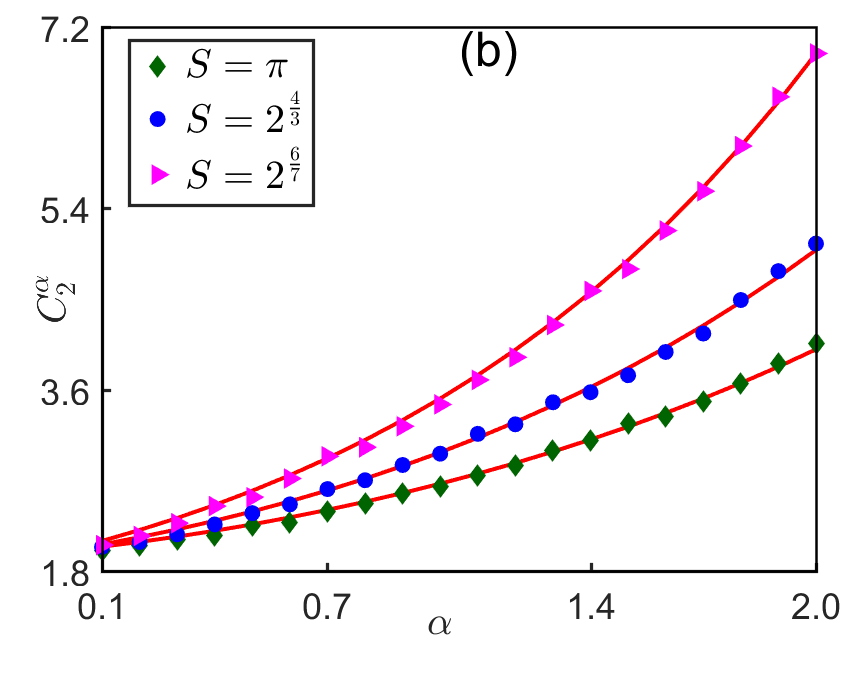
Figure 18: Numerical results of $C_{2}^{\alpha}$ (symbols denote numerical results and solids lines are from fitting formula) for different areas $S=|\Omega|=4L_{2}$ and $\alpha$: (a) plots of $C_{2}^{\alpha}$ as a function of $S$ for different $\alpha$, and (b) plots of $C_{2}^{\alpha}$ as a function of $\alpha$ for different $S$.

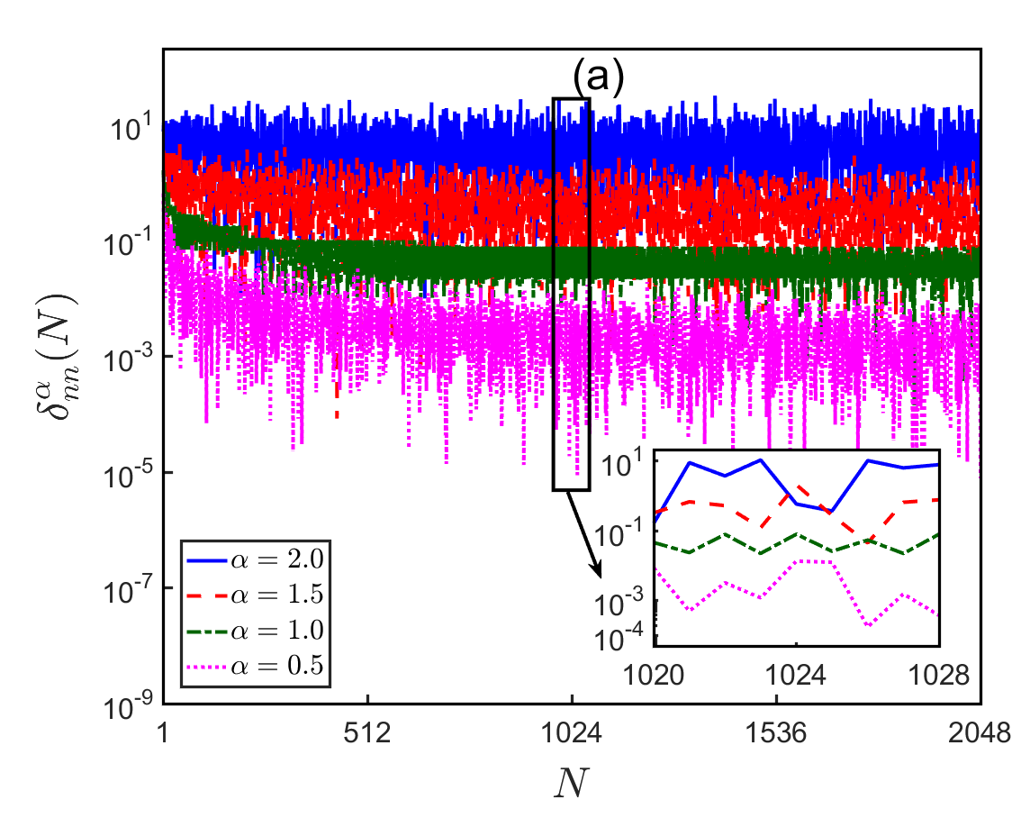
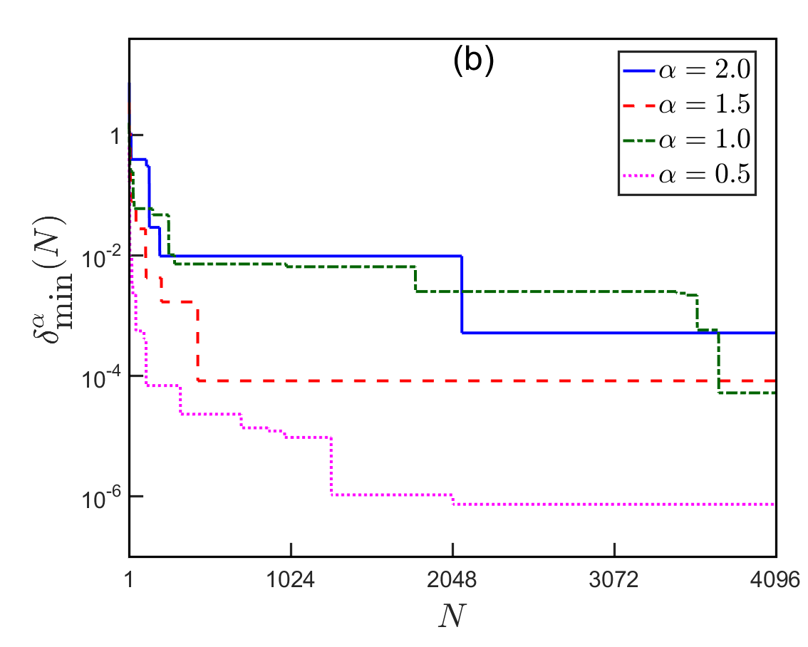
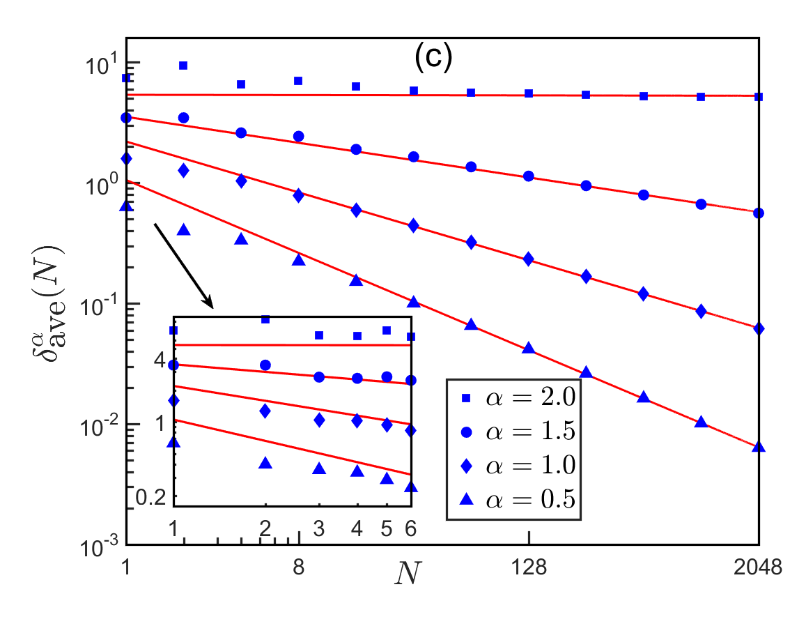
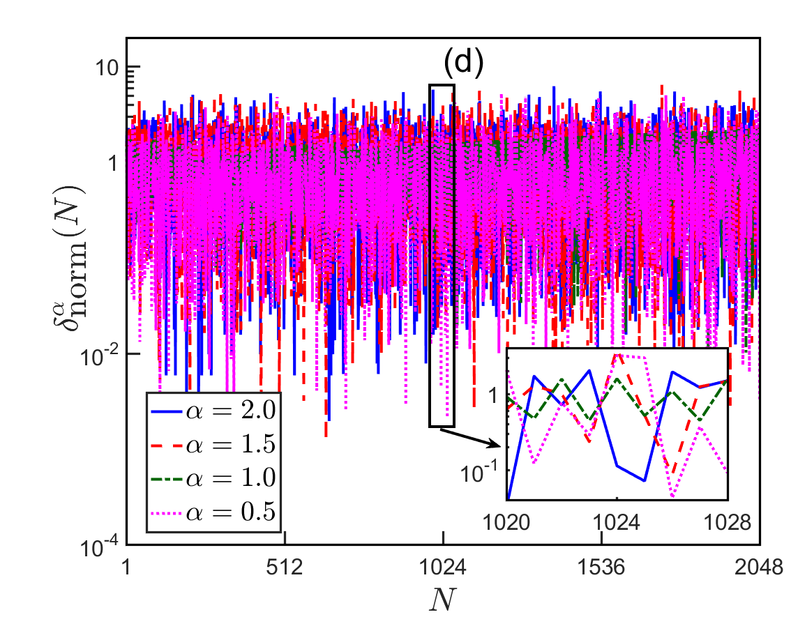
Figure 19: Different eigenvalue gaps of (6.1) with $d=2$, $L_{1}=1$, $V({\bf x})\equiv 0$, $L_{2}=\frac{\sqrt[3]{2}}{2}$ and different $\alpha$ for: (a) the nearest neighbour gaps $\delta_{\rm nn}^{\alpha}(N)$, (b) the minimum gaps $\delta_{\textrm{min}}^{\alpha}(N)$, (c) the average gaps $\delta_{\textrm{ave}}^{\alpha}(N)$ (symbols denote numerical results and solids lines are from fitting formula when $N\gg 1$), and (d) the normalized gaps $\delta_{\rm norm}^{\alpha}(N)$.

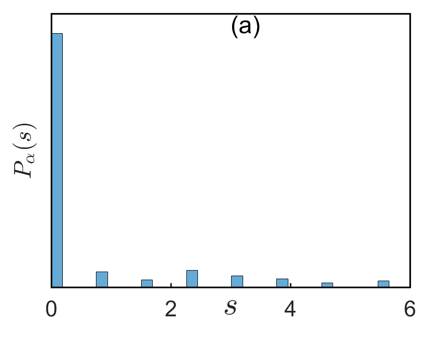
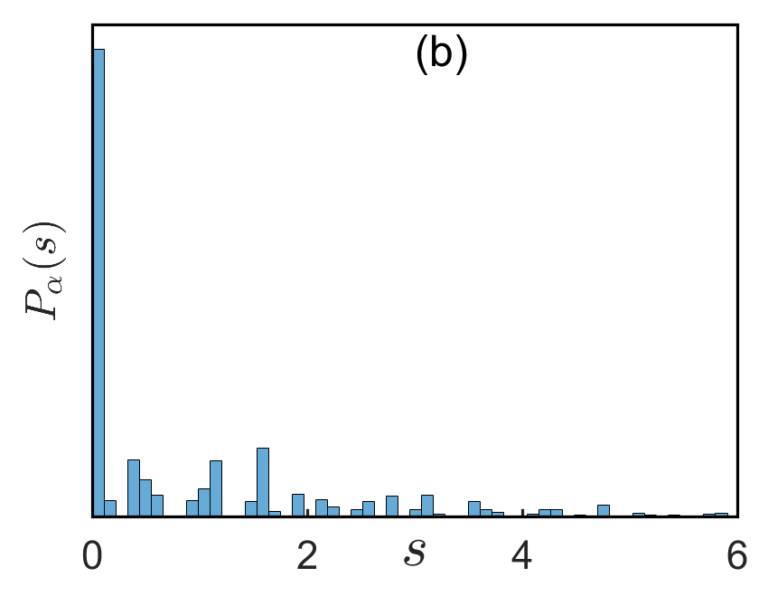
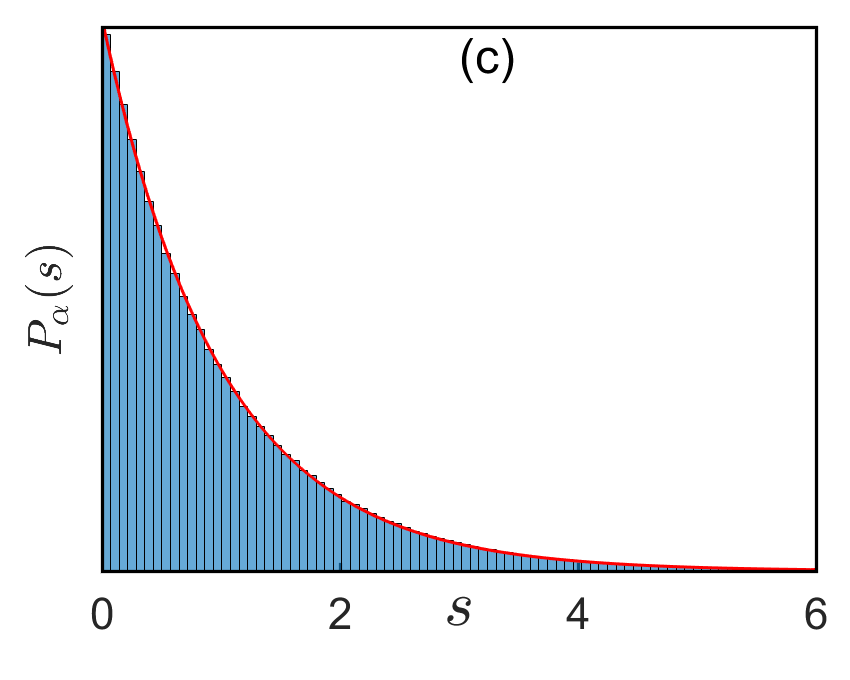
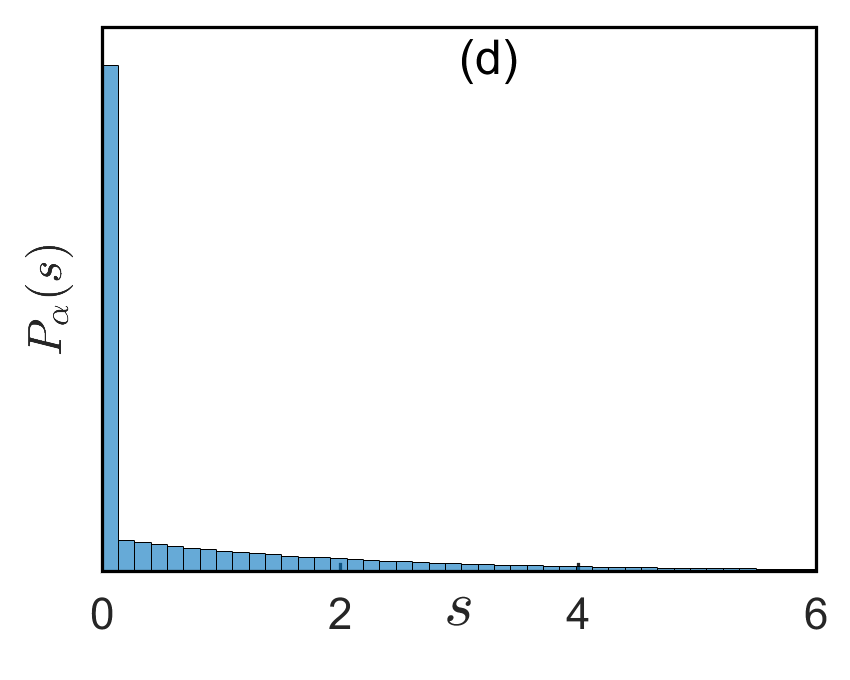
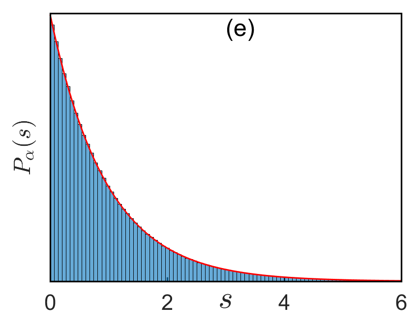
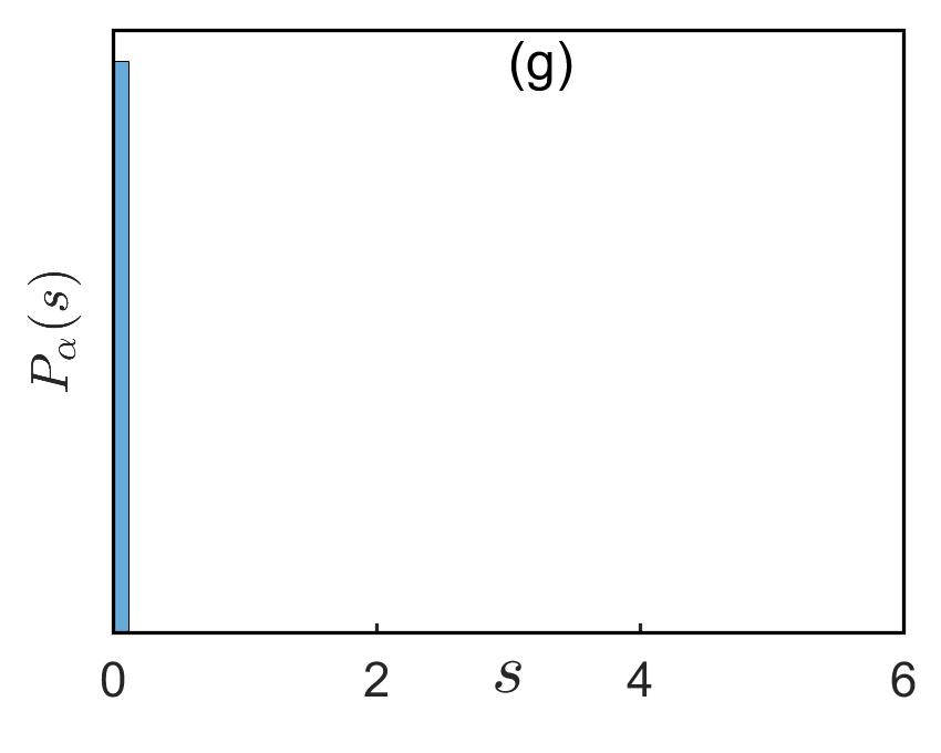
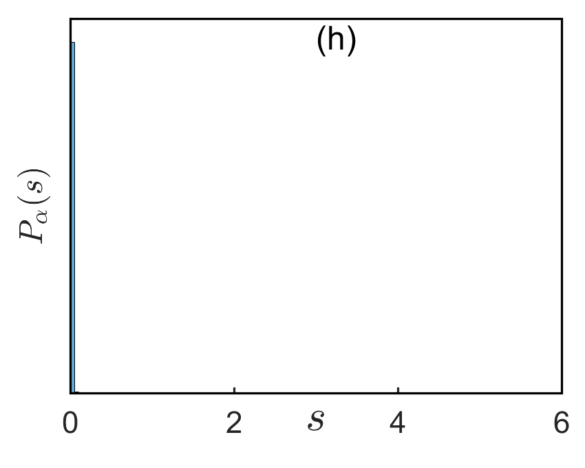
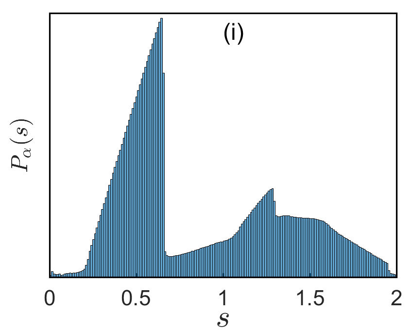
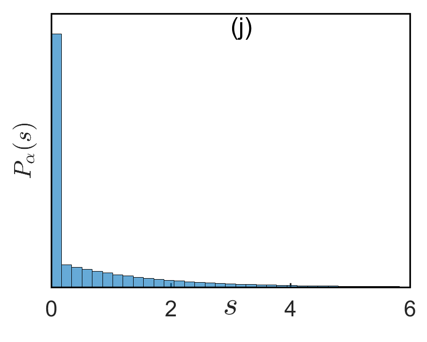
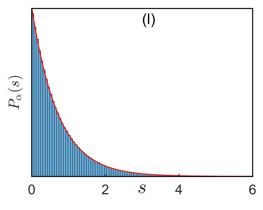
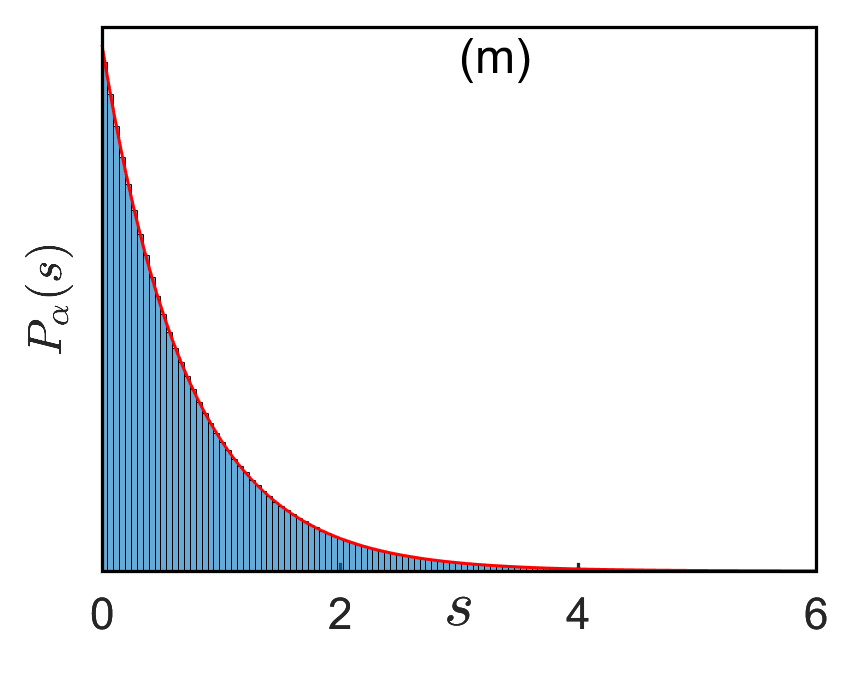
Figure 20: The histogram of the normalized gaps $\{\delta_{\rm norm}^{\alpha}(n)\ |\ 1\leq n\leq N=4000000\}$ of (6.1) with $d=2$, $L_{1}=1$ and $V({\bf x})\equiv 0$ for different $0<\alpha\leq 2$ and $0<L_{2}\leq 1$: (a) $\alpha=2.0$ and $L_{2}=1$, (b) $\alpha=2.0$ and $L_{2}=2/3$, (c) $\alpha=2.0$ and $L_{2}=\frac{\sqrt[3]{2}}{2}$; (d) $\alpha=1.5$ and $L_{2}=1$, (e) $\alpha=1.5$ and $L_{2}=2/3$, (f) $\alpha=1.5$ and $L_{2}=\frac{\sqrt[3]{2}}{2}$; (g) $\alpha=1.0$ and $L_{2}=1$, (h) $\alpha=1.0$ and $L_{2}=2/3$, (i) $\alpha=1.0$ and $L_{2}=\frac{\sqrt[3]{2}}{2}$; (j) $\alpha=0.5$ and $L_{2}=1$, (l) $\alpha=0.5$ and $L_{2}=2/3$, (m) $\alpha=0.5$ and $L_{2}=\frac{\sqrt[3]{2}}{2}$. Solid lines are fitting curves for the gaps distribution statistics $P_{\alpha}(s)$.

6.2 Numerical results in two dimensions (2D) without potential

We take $d=2$, $L_{1}=1$ and $V({\bf x})\equiv 0$ in (6.1). In this case, noting (6.4) and (6.5) with $d=2$, instead of using the JSM in 2D to compute eigenvalues and their corresponding eigenfunctions of (6.1), a simple and more efficient and accurate way is to first use the JSM in 1D to compute the eigenvalues and their corresponding eigenfunctions of (1.1) with $\Omega=(-1,1)$ and $V(x)\equiv 0$, and then to get the eigenvalues and their corresponding eigenfunctions of (6.1) with $d=2$ and $V({\bf x})\equiv 0$ via (6.4) and (6.5) with $d=2$.

In our computations, we first use the JSM in 1D with $M=8192$ to compute numerically the eigenvalues of (1.1) with $\Omega=(-1,1)$ and $V(x)\equiv 0$. Then we use the first $N=4096$ computed eigenvalues to get the eigenvalues of (6.1) with $d=2$ and $V({\bf x})\equiv 0$ via (6.4) with $d=2$ and then rank (or order) the total $4096\times 4096$ eigenvalues of (6.1) as (1.4). Finally, we take (up to) the first $N=4000000$ eigenvalues to compute the gaps and their distribution statistics.

Figure 17 displays eigenvalues (in increasing order) of (6.1) for different $L_{2}$ and $\alpha$, which suggests that $\lambda_{n}^{\alpha}\sim n^{\alpha/2}$ when $n\gg 1$ for $0<\alpha\leq 2$. Then we fit numerically $\lambda_{n}^{\alpha}$ when $n\gg 1$ by $C_{2}^{\alpha}n^{\alpha/2}$. Figure 18 displays the fitting results of $C_{2}^{\alpha}$ with respect to the area $S=4L_{2}$ of $\Omega$ and $\alpha$, which suggests that

$$C_{2}^{\alpha}=\frac{4}{2+\alpha}\left(\frac{4\pi}{S}\right)^{\alpha/2},\qquad 0<\alpha\leq 2,\qquad S=4L_{2}>0.$$ (6.7)

These results immediately suggest that

$$\lambda_{n}^{\alpha}=\frac{4}{2+\alpha}\left(\frac{4\pi}{S}\right)^{\alpha/2}\;n^{\alpha/2}+o(n^{\alpha/2}),\qquad n\gg 1.$$ (6.8)

Specifically, when $\alpha=2$, our numerical results suggest that

$$\lambda_{n}^{\alpha=2}=\frac{4\pi}{S}\left[n+C_{1}n^{1/2}+O(1)\right],\qquad n\gg 1,$$ (6.9)

where $C_{1}\approx 0.5943$ from our numerical results. In fact, (6.9) can be regarded as an improved Weyl law when $\alpha=2$ [60], and (6.8) can be regarded as an extension of the Weyl law for $\alpha=2$ [60] to $0<\alpha\leq 2$, and we call (6.8) as the generalized Weyl law on the asymptotics of the eigenvalues of the D-FSO in 2D.

In fact, combining (6.8) and (1.7), we can obtain the asymptotic of the average gaps of the D-FSO in (6.1) as

$$\delta_{\rm ave}^{\alpha}(N) = \frac{\lambda_{N+1}^{\alpha}-\lambda_{1}^{\alpha}}{N}$$ (6.10)

$$= \frac{1}{N}\left[\frac{4}{2+\alpha}\left(\frac{4\pi}{S}\right)^{\alpha/2}\;(N+1)^{\alpha/2}+o((N+1)^{\alpha/2})-\lambda_{1}^{\alpha}\right]$$

$$= \frac{4}{2+\alpha}\left(\frac{4\pi}{S}\right)^{\alpha/2}N^{(\alpha-2)/2}+o(N^{(\alpha-2)/2})$$

$$= O(N^{(\alpha-2)/2}),\qquad N\gg 1,$$

which immediately implies that, when $\alpha=2$, $\delta_{\rm ave}^{\alpha}(N)\sim 1$ (i.e. almost a constant) when $N\gg 1$, and respectively, when $0<\alpha<2$, $\delta_{\rm ave}^{\alpha}(N)\sim N^{(\alpha-2)/2}$ (decrease with respect to $N$) when $N\gg 1$.

In addition, Figure 19 plots different eigenvalue gaps of (6.1) with $d=2$, $L_{1}=1$, $V({\bf x})\equiv 0$, $L_{2}=\sqrt[3]{2}/2$ and different $\alpha$. Figure 20 displays the histogram of the normalized gaps $\{\delta_{\rm norm}^{\alpha}(n)\ |\ 1\leq n\leq N=4000000\}$ for different $\alpha$ and $L_{2}$. Figure 21 plots $1-R^{\alpha}(N)$ vs $N$ ($N\gg 1$) for different $\alpha$ and $L_{2}$.

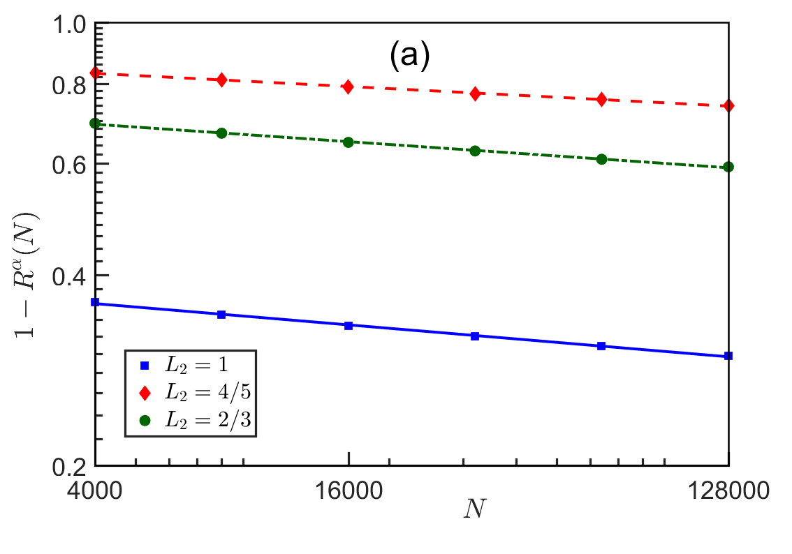
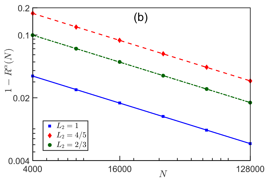
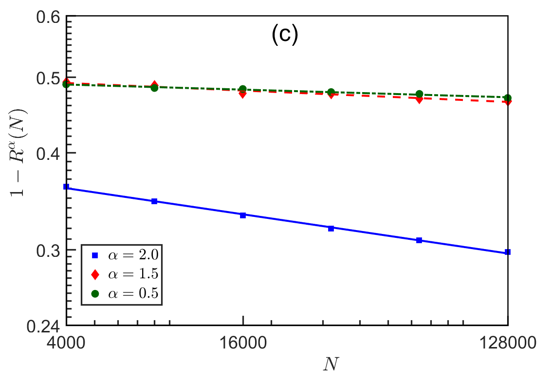
Figure 21: Plots of $1-R^{\alpha}(N)$ vs $N$ ($N\gg 1$) for different $\alpha$ and $L_{2}$: (a) $\alpha=2$ for different $L_{2}\in{\mathbb{Q}}$; (b) $\alpha=1$ for different $L_{2}\in{\mathbb{Q}}$; and (c) $L_{2}=1$ for different $0<\alpha\leq 2$.

From Figs. 19-21, we can draw the following conclusions:

(i) The minimum gaps $\delta_{\rm min}(N)\to 0$ when $N\to+\infty$ (cf. Fig. 19b); and the average gaps $\delta_{\rm ave}(N)\sim 1$ when $N\gg 1$ for $\alpha=2$, and respectively, $\delta_{\rm ave}(N)\sim N^{(\alpha-2)/2}$ when $N\gg 1$ for $0<\alpha<2$ (cf. Fig. 19c), which confirm the asymptotic results in (6.10).

(ii) When $L_{2}=1$ and $0<\alpha\leq 2$ or $\alpha=2$ and $L_{2}\in{\mathbb{Q}}$ or $\alpha=1$ and $L_{2}\in{\mathbb{Q}}$, the gaps distribution statistics $P_{\alpha}(s)=\delta(s)$ (cf. Fig. 20a,b,d,g,h,j and Fig. 21). In these cases, $R^{\alpha}(N)\to 1$ when $N\to\infty$ (cf. Fig. 21) and our numerical results suggest the following asymptotics: $R^{\alpha}(N)=1-N^{-\tau_{2}(L_{2})}$ when $\alpha=2$ for different $L_{2}\in{\mathbb{Q}}$ (cf. Fig. 21a); $R^{\alpha}(N)=1-N^{-1/2}$ when $\alpha=1$ for different $L_{2}\in{\mathbb{Q}}$ (cf. Fig. 21b); and $R^{\alpha}(N)=1-N^{-\tau_{3}(\alpha)}$ when $L_{2}=1$ for different $0<\alpha\leq 2$ (cf. Fig. 21c). In addition, Figure 22 plots $\tau_{2}(L_{2})$ and $\tau_{3}(\alpha)$ based on our numerical results.

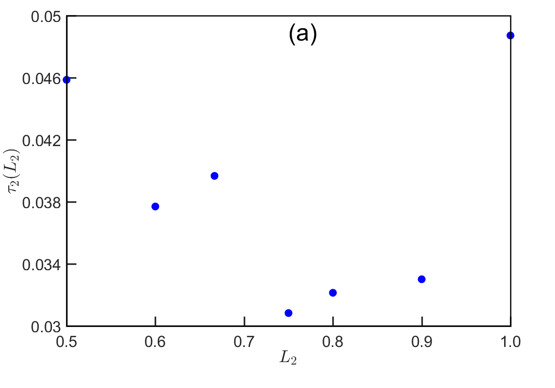
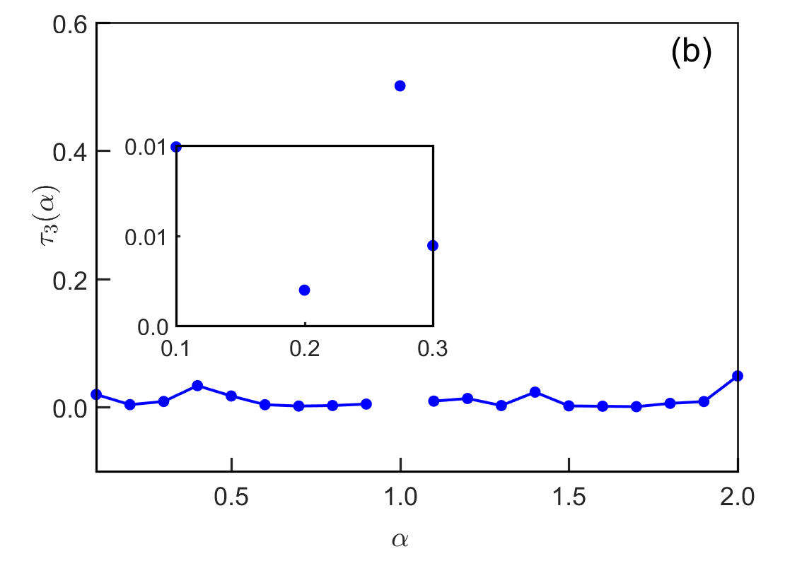
Figure 22: Fitting results of $\tau_{2}(L_{2})$ for different $L_{2}\in{\mathbb{Q}}$ (left) and $\tau_{3}(\alpha)$ for different $\alpha$ (right).

(iii) When $L_{2}\notin{\mathbb{Q}}$ and $0<\alpha<1$ or $1<\alpha\leq 2$, $P_{\alpha}(s)$ can be well approximated by a Poisson distribution (cf. Fig. 20c,e,f,l,m), i.e.

$$P_{\alpha}(s)=\tau(\alpha)e^{-\tau(\alpha)\,s},\qquad s\geq 0.$$ (6.11)

In addition, Figure 23 plots $\tau(\alpha)$, which suggests that

$$\tau(\alpha)\approx\left\{\begin{array}[]{ll}1,&1<\alpha\leq 2,\\ 1.057\alpha^{-0.385},&0<\alpha<1.\\ \end{array}\right.$$ (6.12)

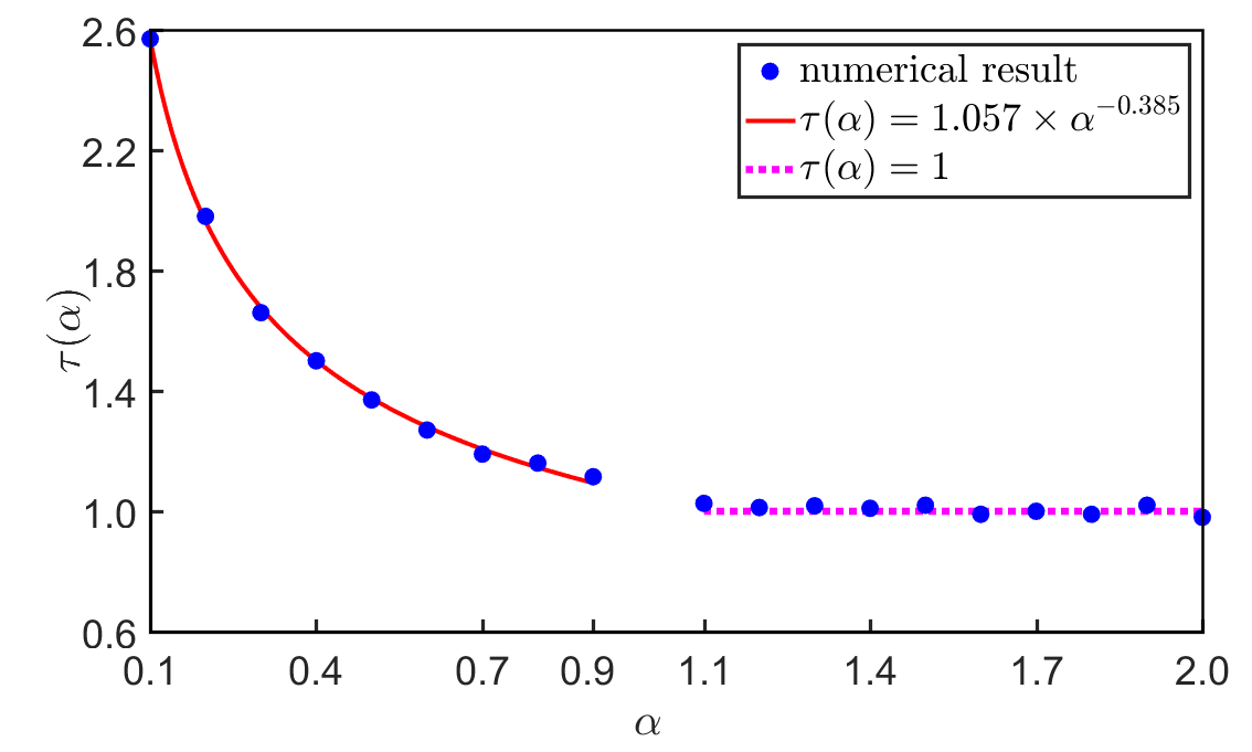
Figure 23: Fitting results of $\tau(\alpha)$ for different $\alpha$.

(iv) When $\alpha=1$ and $L_{2}\notin{\mathbb{Q}}$, $P_{\alpha}(s)$ can be well approximated by a bimodal distribution [48] (cf. Fig. 20i).

(v) The classification of the gaps distribution statistics $P_{\alpha}(s)$ for different $0<\alpha\leq 2$ and $L_{1}>0$ and $L_{2}>0$ is summarized in Table 6.

	$L_{2}/L_{1}=1$	$1\neq L_{2}/L_{1}\in{\mathbb{Q}}$	$1\neq L_{2}/L_{1}\notin{\mathbb{Q}}$
$\alpha=2$	$\delta(s)$	$\delta(s)$	Poisson
$1<\alpha<2$	$\delta(s)$	Poisson	Poisson
$\alpha=1$	$\delta(s)$	$\delta(s)$	Bimodal distribution
$0<\alpha<1$	$\delta(s)$	Poisson	Poisson

Table 6: Summary of the eigenvalue gap distribution statistics of (6.1) with $d=2$ and $V({\bf x})\equiv 0$ for different $0<\alpha\leq 2$ and $L_{1}>0$ and $L_{2}>0$.

6.3 Numerical results in 2D with potential

Here we use the JSM in 2D to compute numerically the eigenvalues and their corresponding eigenfunctions of (6.1) with $d=2$ and a non-zero potential $V(x,y)$. In our computations, we choose the total DOF $M=144\times 144$, i.e. with DOFs $M_{1}=144$ and $M_{2}=144$ in $x_{1}$ and $x_{2}$ directions, respectively. With the $M$ eigenvalues computed, we only use $M/4$ (or even less) numerical eigenvalues to compute gaps and their distribution statistics. We take $L_{1}=1$ and $V(x,y)=\frac{x^{2}+y^{2}}{2}$ in (6.1).

Figure 24 plots different eigenvalue gaps of (6.1) with $L_{2}=\sqrt[3]{2}/2$ for different $\alpha$, and Figure 25 displays the histogram of the normalized gaps $\{\delta_{\rm norm}^{\alpha}(n)\ |\ 1\leq n\leq N=4096\}$ for different $\alpha$ and $L_{2}$.

We also carry out numerical simulations on eigenvalues and their different gaps as well as their distribution statistics of (6.1) in 2D with different other potentials. Our numerical results suggest that the asymptotic behavior of the eigenvalue $\lambda_{n}^{\alpha}$ in (6.8) and (6.9) are still valid when (6.1) is with a potential $V({\bf x})\in C(\Omega)$. In addition, similar to the 1D case, the gaps and their distribution statistics of (6.1) with a potential are quite similar to those without potential, which are reported in Figs. 19&20. Those numerical results are omitted here for brevity.

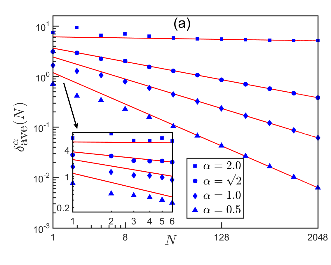
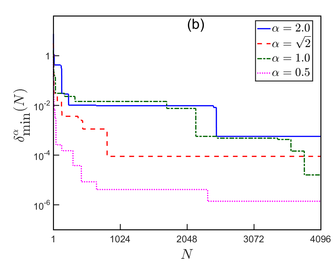
Figure 24: Different gaps of (6.1) with $d=2$, $L_{1}=1$, $L_{2}=\sqrt[3]{2}/2$ and $V(x,y)=\frac{x^{2}+y^{2}}{2}$: (a) the average gaps $\delta_{\textrm{ave}}^{\alpha}(N)$, and (b) the minimum gaps $\delta_{\textrm{min}}^{\alpha}(N)$ (symbols denote numerical results and solids lines are from fitting formula when $N\gg 1$).

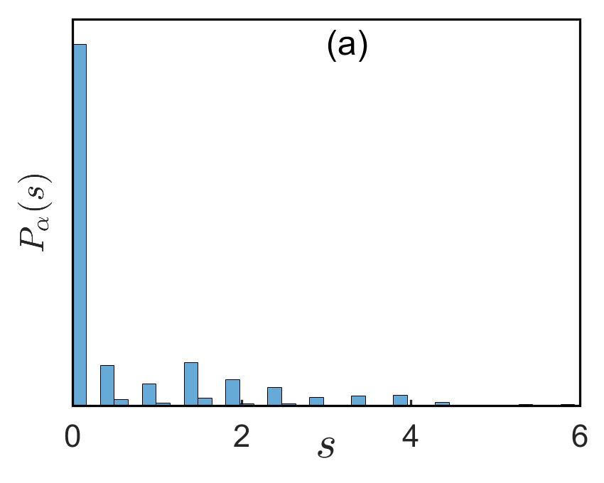
Figure 25: The histogram of the normalized gaps $\{\delta_{\rm norm}^{\alpha}(n)\ |\ 1\leq n\leq N=4096\}$ of (6.1) with $d=2$ and $V(x,y)=\frac{x^{2}+y^{2}}{2}$: (a) $\alpha=2$ and $L_{2}=1$; and (b) $\alpha=\sqrt{2}$ and $L_{2}=\sqrt[3]{2}/2$ (the solid line is a fitting curve by the Poisson distribution).

Finally, based on our extensive numerical results and observations, we speculate the following observation (or conjecture) for the D-FSO in (6.1) without/with potential:

Conjecture III (Gaps and their distribution statistics of D-FSO in (6.1) with $d=2$) Assume $0<\alpha\leq 2$ and $V(x)\in C(\bar{\Omega})$ in (6.1), then we have the following asymptotics of its eigenvalues:

$$\lambda_{n}^{\alpha}=\frac{4}{2+\alpha}\left(\frac{4\pi}{S}\right)^{\alpha/2}\;n^{\alpha/2}+o(n^{\alpha/2}),\qquad n\gg 1,$$ (6.13)

where $S$ is the area of $\Omega$. In addition, we have the following asymptotics of different gaps:

$$\begin{split}&\delta_{\rm min}^{\alpha}(N)\to 0,\qquad N\to+\infty,\\ &\delta_{\rm ave}^{\alpha}(N)=\frac{4}{2+\alpha}\left(\frac{4\pi}{S}\right)^{\alpha/2}N^{(\alpha-2)/2}+o(N^{(\alpha-2)/2}),\qquad N\gg 1.\end{split}$$ (6.14)

In addition, the gap distribution statistics summarized in Tab. 6 is also valid for (6.1) in 2D with the potential $V$.

7 Conclusion

We proposed a Jacobi-Galerkin spectral method for accurately computing a large amount of eigenvalues of the fractional Schrödinger operator (FSO). A very important advantage of the proposed numerical method is that, under a fixed number of degree of freedoms $M$, the Jacobi spectral method can calculate accurately a large number of eigenvalues with the number proportional to $M$. Based on the eigenvalues obtained numerically by the proposed method, we obtained several important and interesting results for the eigenvalues and their different gaps of FSO in 1D and directional FSO in 2D. Based on the gaps, the distribution statistics of the normalized gaps were obtained numerically for the FSO.

Acknowledgment

The first author thanks very stimulating discussion with Professor Zeev Rudnick. This work was partially support by the Ministry of Education of Singapore grant R-146-000-290-114 (W. Bao), the National Natural Science Foundation of China Grants 11671166 (L.Z. Chen), U1930402 (L.Z. Chen & Y. Ma) and 11771254 (X.Y. Jiang). Part of the work was done when the authors were visiting the Institute for Mathematical Sciences at the National University of Singapore in 2019 (W. Bao and Y. Ma).

References

References

- [1] B. Andrews, J. Clutterbuck, Proof of the fundamental gap conjecture, J. Am. Math. Soc. 24 (2010) 899–916.
- [2] X. Antoine, Q.L. Tang, Y. Zhang, On the ground states and dynamics of space fractional nonlinear Schrödinger/Gross-Pitaevskii equations with rotation term and nonlocal nonlinear interactions, J. Comput. Phys. 325 (2016) 74-97.
- [3] M.S. Ashbaugh, R. Benguria, Optimal lower bound for the gap between the first two eigenvalues of one-dimensional Schrödinger operators with symmetric single-well potentials, Proc. Amer. Math. Soc. 105 (1989) 419–424.
- [4] P. Bader, S. Blanes, F. Casas, Solving the Schrödinger eigenvalue problem by the imaginary time propagation technique using splitting methods with complex coefficients, J. Chem. Phys. 139 (2013) 124117.
- [5] W. Bao, N. Ben Abdallah, Y. Cai, Gross-Pitaevskii-Poisson equations for dipolar Bose-Einstein condensate with anisotropic confinement, SIAM J. Math. Anal. 44 (2012) 1713-1741.
- [6] W. Bao, X. Dong, Numerical methods for computing ground state and dynamics of nonlinear relativistic Hartree equation for boson stars, J. Comput. Phys. 230 (2011) 5449-5469.
- [7] W. Bao, H. Jian, N. J. Mauser, Y. Zhang, Dimension reduction of the Schrödinger equation with Coulomb and anisotropic confining potentials, SIAM J. Appl. Math. 73 (2013) 2100-2123.
- [8] W. Bao, X. Ruan, Fundamental gaps of the Gross-Pitaevskii equation with repulsive interaction, Asymptot. Anal. 110 (2018) 53-82.
- [9] W. Bao, X. Ruan, J. Shen, C. Sheng, Fundamental gaps of the fractional Schrödinger operator, Commun. Math. Sci. 17 (2019) 447-471.
- [10] M.V.D. Berg, On condensation in the free-boson gas and the spectrum of the Laplacian, J. Stat. Phys. 31 (1983) 623–637.
- [11] C. Bernardi, Y. Maday, Spectral methods, Handb. Numer. Anal. 5 (1997), 209-485.
- [12] D. Boffi, Finite element approximation of eigenvalue problems, Acta Numer. 19 (2010) 1-120.
- [13] A. Bonito, J.P. Borthagaray, R.H. Ricardo, E. Otárola, A.J. Abner, Fundamental gaps of the fractional Schrödinger operator, Comput. Visual. Sci. 19 (2018) 19-46.
- [14] J.P. Borthagaray, L.M. D. Pezzo, S. Mart nez, Finite element approximation for the fractional eigenvalue problem, J. Sci. Comput. 77 (2018) 308-329.
- [15] J. Bourgain, V. Blomerand, Z. Rudnick, Small gaps in the spectrum of the rectangular billiard, Ann. Sci. Éc. Norm. Supér. 50 (2017) 1283–1300.
- [16] L. Caffarelli, L. Silvestre, An extension problem related to the fractional Laplacian, Commun. Part. Differ. Eq. 32 (2007) 1245–1260.
- [17] Y. Cai, M. Rosenkranz, Z. Lei, W. Bao, Mean-field regime of trapped dipolar Bose-Einstein condensates in one and two dimensions, Phys. Rev. A 82 (2010) 043623.
- [18] L. Carusotto, C. Citui, Quantum fluids of lights, Rev. Mod. Phys., 85 (2013) 299.
- [19] C. Çelik, M. Duman, Crank-Nicolson method for the fractional diffusion equation with the Riesz fractional derivative, J. Comput. Phys. 231 (2012) 1743–1750.
- [20] S.L. Chang, C.S. Chien, B.W. Jeng, An efficient algorithm for the Schrödinger-Poisson eigenvalue problem, J. Comput. Appl. Math. 205 (2007) 509-532.
- [21] L.Z. Chen, Z.P. Mao, H.Y. Li, Jacobi-Galerkin spectral method for eigenvalue problems of Riesz fractional differential equations, arXiv:1803.03556.
- [22] Z.Q. Chen, R. Song, Two sided eigenvalue estimates for subordinate processes in domains. J. Funct. Anal. 226 (2005) 90–113.
- [23] S. Costiner, S. Ta’asan, Simultaneous multigrid techniques for nonlinear eigenvalue problems: Solutions of the nonlinear Schrödinger-Poisson eigenvalue problem in two and three dimensions, Phys. Rev. E 52 (1995) 1181.
- [24] M. D’Elia, M. Gunzburger, The fractional Laplacian operator on bounded domains as a special case of the nonlocal diffusion operator, Comput. Math. Appl. 66 (2013) 1245–1260.
- [25] Q. Du, M. Gunzburger, R.B. Lehoucq, K. Zhou, Analysis and approximation of nonlocal diffusion problems with volume constraints, SIAM Rev. 54 (2012) 667–696.
- [26] S.W. Duo, Y.Z. Zhang, Computing the ground and first excited states of the fractional Schrödinger equation in an infinite potential well, Commun. Comput. Phys. 18 (2015) 321–350.
- [27] B. Dyda, Fractional calculus for power functions and eigenvalues of the fractional Laplacian, Fract. Calc. Appl. Anal. 15 (2012) 536-555.
- [28] A. Elgart, B. Schlein, Mean field dynamics of boson stars, Commun. Pure Appl. Math. 60 (2007) 500-545.
- [29] W.P. Fan, F.W. Liu, X.Y. Jiang, I. Tumer, A novel unstructured mesh finite element method for solving the time-space fractional wave equation on a two-dimensional irregular convex domain, Fract. Calc. Appl. Anal. 20 (2017) 352–383.
- [30] P. Grisvard, Elliptic Problems in Nonsmooth Domains, Pitman Advanced Pub, Boston, 1985.
- [31] G. Grubb, Fractional Laplacians on domains, a development of Hörmander’s theory of -transmission pseudodifferential operators, Adv. Math. 268 (2015) 478-528.
- [32] E.M. Harrell, Commutators, eigenvalue gaps, and mean curvature in the theory of Schrödinger operators, Commun. Part. Diff. Eq. 32 (2007) 401-413.
- [33] D. Jakobson, S. Miller, I. Rivin, Z. Rudnick, Level spacings for regular graphs, IMA Math. Appl. 109 (1999) 317-329.
- [34] S. Jiang, L. Greengard, W. Bao, Fast and accurate evaluation of nonlocal Coulomb and dipole-dipole interactions via the nonuniform FFT, SIAM J. Sci. Comput. 36 (2014) B777-B794.
- [35] B.T. Jin, R. Lazarov, J. Pasciak, W. Rundell, A finite element method for the fractional Sturm-Liouville problem, arXiv: 1307.5114.
- [36] M. Kwaśnicki, Ten equivalent definitions of the fractional Laplace operator, Fract. Calc. Appl. Anal. 20 (2017) 7-51.
- [37] M. Kwaśnicki, Eigenvalues of the fractional Laplace operator in the interval, J. Funct. Anal. 262 (2012) 2379–2402.
- [38] P. Li, S.T. Yau, On the Schrödinger equation and the eigenvalue problem, Commun. Math. Phys. 88 (1983) 309-318.
- [39] J.L. Lions, E. Magenes, Non-homogeneous Boundary Value Problems and Applications, Springer-Verlag, 1972.
- [40] A. Lischke, G.F. Pang, M. Gulian, F.Y. Song, C. Glusa, X.N. Zheng, Z.P. Mao, W. Cai, M.M. Meerschaert, M. Ainsworth, What is the fractional Laplacian? arxiv: 1801.09767.
- [41] F.W Liu, S.P. Chen, I. Turner, K. Burrage, V. Anh, Numerical simulation for two-dimensional Riesz space fractional diffusion equations with a nonlinear reaction term, Cent. Eur. J. Phys. 11 (2013) 1221–1232.
- [42] O.E. Livne, A. Brandt, Multiscale Eigenbasis Calculations: Eigenfunctions in O(N log N), Springer Berlin Heidelberg, 2002.
- [43] Y. Luchko, Fractional Schrödinger equation for a particle moving in a potential well, J. Math. Phys. 54 (2013) 012111.
- [44] Z.P. Mao, S. Chen, J. Shen, Efficient and accurate spectral method using generalized Jacobi functions for solving Riesz fractional differential equations, Appl. Numer. Math. 106 (2016) 165-181.
- [45] Z.P. Mao, J. Shen, Efficient spectral-Galerkin methods for fractional partial differential equations with variable coefficients, J. Comput. Phys. 307 (2016) 243-261.
- [46] C. Mehl, S. Borm, Numerical Methods for Eigenvalue Problems, 2008.
- [47] E. Di Nezza, G. Palatucci, E. Valdinoci, Hitchhiker’s guide to the fractional Sobolev spaces, Bull. Sci. Math. 136 (2012) 521-573.
- [48] S. Offermanns, W. Rosenthal, Bimodal Distribution, Springer Berlin Heidelberg, 76 (2008) 259-259.
- [49] K.M. Owolabi, A. Atangana, Numerical solution of fractional-in-space nonlinear Schrödinger equation with the Riesz fractional derivative, Eur. Phys. J. Plus 131 (2016) 335.
- [50] F. Pinsker, W. Bao, Y. Zhang, H. Ohadi, A. Dreismann, J.J. Baumberg, Fractional quantum mechanics in polariton condensates with velocity dependent mass, Phys. Rev. B 92 (2015) 195310.
- [51] I. Podlubny, Fractional Differential Equations, Academic Press, San Diego, 1999.
- [52] A. Quarteroni, A. Valli, Numerical Approximation of Partial Differential Equations, Springer Berlin Heidelberg, 1994.
- [53] S.Y. Reutskiy, A new numerical method for solving high-order fractional eigenvalue problems, J. Comput. Appl. Math. 317 (2017) 603-623.
- [54] Z. Rudnick, A metric theory of minimal gaps, Numer. Algor. 64 (2018) 628-636.
- [55] Z. Rudnick, A. Zaharescu, The distribution of spacings between fractional parts of lacunary sequences, Forum Math. 14 (2002) 691-712.
- [56] S.G. Samko, A.A. Kilbas, O.I. Marichev, Fractional Integrals and Derivatives, Gordon and Breach Science Publishers, Yverdon, 1993.
- [57] J. Shen, T. Tang, L.L. Wang, Spectral Methods: Algorithms, Analysis and Applications, Springer Publishing Company, 2011.
- [58] E. Valdinoci, From the long jump random walk to the fractional Laplacian, Bol. Soc. Esp. Mat. Apl. SeMA 49 (2009) 33-44.
- [59] J.A.C. Weideman, L.N. Trefethen, The eigenvalues of second-order spectral differentiation matrices, SIAM J. Numer. Anal. 25 (1988) 1279-1298.
- [60] H.Weyl, Das asymptotische Verteilungsgesetz der Eigenwerte linearer partieller Differentialgleichungen. Mathh. Ann. 71(1912) 441-479.
- [61] F. Zeng, F. Liu, C. Li, K. Burrage, I. Turner, V. Anh, A Crank–Nicolson ADI spectral method for a two-dimensional Riesz space fractional nonlinear reaction-diffusion equation, SIAM J. Numer. Anal. 52 (2014) 2599-2622.
- [62] X. Zhao, Z. Sun, H.Z. Peng, A fourth-order compact ADI scheme for two-dimensional nonlinear space fractional Schrödinger equation, SIAM J. Sci. Comput. 36 (2014) A2865-A2886.
- [63] A. Zoia, A. Rosso, M. Kardar, Fractional Laplacian in bounded domains, Phys. Rev. E 76 (2007) 021116.