Region crossing change on spatial theta-curves
Abstract
A region crossing change at a region of a spatial-graph diagram is a transformation changing every crossing on the boundary of the region. In this paper, it is shown that every spatial graph consisting of theta-curves can be unknotted by region crossing changes.
1 Introduction
A knot is an embedding of a circle in , and a link is an embedding of some circles in . A spatial graph is an embedding of a graph in . A diagram of a knot, link or spatial graph is a projection of to with over/under information at each crossing, where each crossing is made of two arcs intersecting transversely. A knot, link or spatial graph is unknotted, or trivial, if has a diagram which has no crossings. It is well-known that any diagram of a knot or link can be transformed into a diagram of a trivial knot or link by a finite number of crossing changes, where a crossing change is a local transformation shown in Figure 1111Some spatial graphs cannot be unknotted by crossing changes, such as the complete graph . .
A region crossing change at a region of a diagram of a knot, link or spatial graph is a local transformation which yields crossing changes at all the crossings on the boundary of the region. For knots, the following theorem is shown:
Theorem 1.1 ([9]).
Any diagram of any knot can be transformed into a diagram of the trivial knot by a finite number of region crossing changes.
For links, the following is shown:
Theorem 1.2 ([2]).
Any diagram of a link can be transformed into a diagram of a trivial link by a finite number of region crossing changes if and only if is a proper link.
For knots and links, the unknottability on region crossing change does not depend on the choice of diagram.
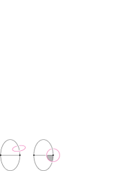
On the other hand, for spatial graphs, it depends on the choice of diagram.
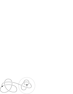
For the two diagrams representing the same spatial graph in Figure 2, the left one cannot be unlinked by region crossing changes at any set of regions, whereas the right one gets unlinked by a region crossing change at the shaded region.
For a spatial graph with a single component, i.e., an embedding of a connected graph, region crossing change is studied in [5]. In this paper, we study region crossing change on a spatial graph with some components, and show the following theorems.
Theorem 1.3.
Let be a two-component spatial graph consisting of a spatial -curve222Spatial -curve is explained in Section 2. and a knot. There exists a diagram of such that can be unknotted by a finite number of region crossing changes.
Theorem 1.4.
Let be a positive integer. Let be an -component spatial graph whose components are all spatial -curves. There exists a diagram of such that can be unknotted by a finite number of region crossing changes.
The rest of the paper is organized as follows: In Section 2, we review the study of region crossing change on spatial graphs. In Section 3, we prove Theorems 2 and 1.4. In Section 4, we also consider spatial handcuff graphs. In Section 5, we study incidence matrices for spatial--curve diagrams. In Section 6, we consider ineffective sets for spatial--curve diagrams.
2 Spatial-graph diagrams
In this section, we prepare some terms of spatial-graph diagrams regarding that knots and links are included by spatial graphs, and review some results on region crossing change.
A graph is a pair of sets of vertices and edges.
Each connected graph which has at least one vertex has a maximal tree, where a maximal tree is a connected subgraph of which includes no cycles and includes all the vertices of .
Since a spatial graph is an embedding of a graph, every connected spatial graph which has a vertex has a maximal tree.
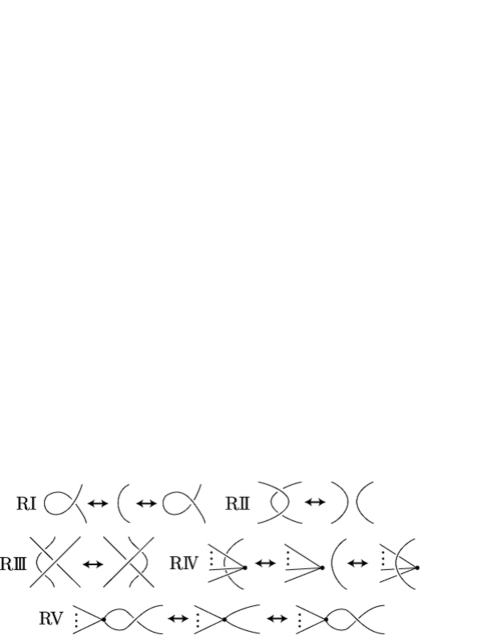
It is known that two diagrams represent the same spatial graph if and only if they are equivalent up to the Riedemeister moves shown in Figure 3.
A crossing of a spatial-graph diagram is reducible if one can draw a circle on such that intersects only transversely as shown in Figure 4. A diagram is said to be reducible if has a reducible crossing. Otherwise, is said to be reduced, or irreducible.
A cutting circle of a diagram is a circle on intersecting an edge transversely at exactly one point as shown in Figure 5. We call such an edge a cutting edge.
For spatial graphs of one component, the following is shown:
Theorem 2.1 ([5]).
Let be a spatial graph of one component, and let be a diagram of without cutting edges. Any crossing change on is realized by a finite number of region crossing changes.
A -curve is a connected graph consisting of two vertices and and three edges which are adjacent to both and . A spatial -curve is an embedding of a -curve in . Since any diagram of a spatial -curve does not have a cutting edge, we have the following:
Lemma 2.2 ([5]).
Any crossing change on any diagram of a spatial -curve is realized by a finite number of region crossing changes.
Theorem 2.1 is a generalization of the following:
Lemma 2.3 ([9]).
Any crossing change on any knot diagram is realized by a finite number of region crossing changes.
3 Proofs of Theorems 2 and 1.4
Proof of Theorem 2. For a spatial graph consisting of a spatial -curve and a knot, take a maximal tree of the -curve component.
Then has a diagram such that the corresponding part of has no crossings (see, for example, [8]).
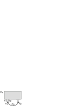
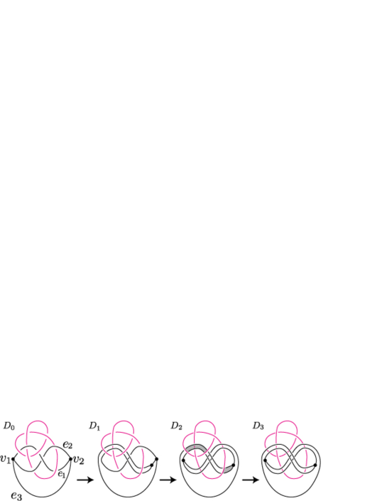
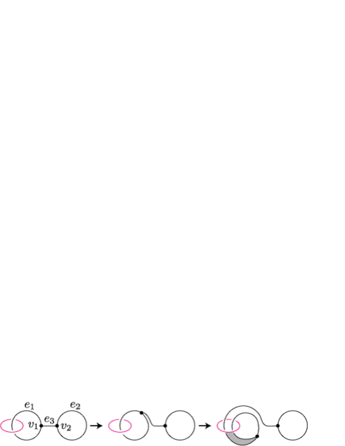
We call the vertices , and edges , and of the -curve component as indicated on in Figure 6.
We note that the maximal tree consists of , and without crossings, and that and may have crossings.
Shrink so that moves to the right side, near , and that and follow making a sufficiently narrow wheel track.
We call the result .
Next, similarly shrink so that moves to the left side, and that and follow making a wheel track, and obtain .
On , the -curve component and the knot component make pairwise crossings at the wheel tracks.
We can change any such crossing pair by region crossing changes as follows:
Let be a crossing pair.
Let be the wheel track where belongs, and let be the adjacent vertex of .
Apply region crossing changes at the regions in the wheel track in order from to .
Then only the crossing pair changes.
Apply region crossing changes on so that the -curve component is over than the knot component at every crossing between them.
An example is shown in Figure 7.
We call the result .
Let be the -curve component diagram in .
Recall that has a set of regions such that is transformed into a diagram of the trivial -curve by region crossing changes at (Lemma 2.2).
Apply region crossing changes on at the regions of corresponding to the regions in .
Then, the -curve component gets unknotted, while crossings between the components are unchanged because there are disjoint four regions around each crossing between them, and an even number of them belongs to .
Thus we obtain a diagram , representing a splittable spatial graph with the -curve component unknotted. Let be the knot component diagram in . Recall that has a set of regions such that is transformed into a diagram of the trivial knot by region crossing changes at (Lemma 2.3). Apply region crossing changes to at the regions of corresponding to the regions in . Then gets unknotted, and crossings between the components are unchanged. Remark that some reducible crossings of may be different from after the region crossing changes while non-reducible crossings are the same. This does not matter since the unknottedness is unchanged even if a reducible crossing is changed. Similarly, the unknottedness of the -curve component is also unchanged. Thus, we obtain a diagram of an unknotted spatial graph by a finite number of region crossing changes from a diagram of .
Next, we prove Theorem 1.4 in a similar way.
Proof of Theorem 1.4. Let be a spatial graph consisting of spatial -curves, and let be a diagram of .
Take a maximal tree for each -curve component.
Gather the maximal trees to the same place in the following way.
Choose a region of .
Take a small part of an edge of each maximal tree, and move it into by Reidemeister moves.
Then move the adjacent vertices into along the edge, by Reidemeister moves.
We call the result , and name the components , vertices and edges as shown in Figure 8.
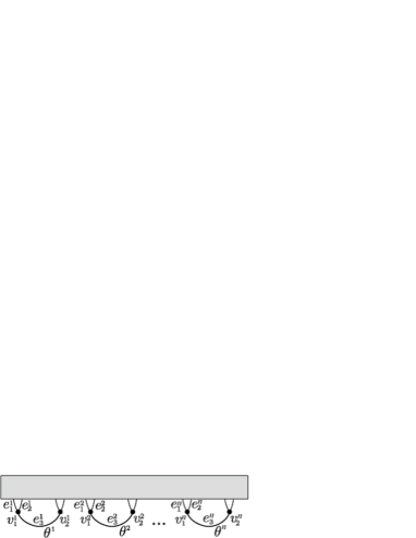
Move to another side near by shrinking for each with an order, where and follow making a wheel track, and we obtain a diagram . Then move to another side by shrinking for each , where and follow making a wheel track. Thus, we obtain a diagram of , and this is the diagram we required.
We can transform into a diagram such that is over than () at each crossing between them by region crossing changes using the wheel-track method of the proof of Theorem 2. We call such a diagram . Each diagram of has a set of regions such that gets unknotted by the region crossing changes by Lemma 2.2. Apply region crossing changes at the corresponding regions in order from to . Then we obtain a diagram of the unknotted spatial graph.
Corollary 3.1.
Let be a spatial graph consisting of some spatial -curves and a proper link. There exists a diagram of such that can be unknotted by a finite number of region crossing changes.
4 Spatial handcuff graphs
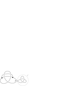
A handcuff graph is a connected graph consisting of two vertices , and two loops based on and , and an edge connecting and . A spatial handcuff graph is an embedding of a handcuff graph in . Similarly to spatial -curve, we can unknot a spatial graph consisting of a spatial handcuff graph and a knot by region crossing change by taking a suitable diagram as shown in Figure 9.
We have the following corollary:
Corollary 4.1.
Let be a two-component spatial graph consisting of a spatial handcuff graph and a knot. There exists a diagram of such that can be unknotted by a finite number of region crossing changes.
Proof.
Let , be the loop edge based on , , respectively, and let be the non-loop edge of the handcuff component. Then , and form a maximal tree of the handcuff component. Take a diagram of such that has no crossings. If the handcuff component in has a cutting edge, apply Reidemeister moves to so that there are no cutting edges, and call the result . Move along until it backs to the initial position, where and makes a wheel track, and we call the result . Similarly, move along and obtain a diagram , and this is the diagram we required. The rest steps are same to the proof of Theorem 2. ∎
We also have the following corollary:
Corollary 4.2.
Let be a spatial graph consisting of some spatial -curves, some spatial handcuff graphs and a proper link. There exists a diagram of such that can be unknotted by a finite number of region crossing changes.
5 Incidence matrices
In this section, we consider incidence matrices, and show the following:
Proposition 5.1.
Let be a diagram of a spatial -curve, and let be a diagram obtained from by crossing changes at some crossings. There exist exactly eight sets of regions of such that is transformed into by region crossing changes at the regions.
We show an example:
Example 5.2.
For the diagram in Figure 10, if one wants to change the crossing , one should solve the following simultaneous equations (see [1] for knots):
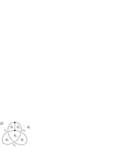
The first equation implies that one should choose an odd number of regions from , , and to change . The second equation implies that one should choose an even number of regions from , , and not to change . For the simultaneous equations, we have eight solutions, and then we have eight sets of regions , , , , , , , to change only by region crossing changes.
Let be a spatial graph, and let be a diagram of . For crossings and regions of , the region choice matrix of is a matrix defined by the following:
We note that the region choice matrix for knots is introduced in [1] not only for modulo 2. We also note that the region choice matrix of modulo 2 is the transposed matrix of the incidence matrix introduced in [3]. The region choice matrix of the diagram in Figure 10 is
and this is equivalent to the coefficient matrix of the simultaneous equation in Example 5.2.
For knots, the size of a region choice matrix of a knot diagram with crossings is , and then it is shown in [3] that the rank is using Lemma 2.3, and the knot version of Proposition 5.1 is shown in [7] and [4] as the number of sets is four. We show Proposition 5.1 in the same way. First, we show the following:
Lemma 5.3.
Let be a diagram of a spatial -curve with crossings. The size of a region choice matrix of is .
Since crossings correspond to the rows, and regions correspond to the columns, Lemma 5.3 follows from the following lemma:
Lemma 5.4.
Every diagram of a spatial -curve has the number of regions three more than the number of crossings.
Proof.
Let be a diagram of a spatial -curve with crossings, and let be a graph obtained from by regarding each crossing to be a vertex. That is, is a graph on with vertices. Looking locally at each vertex of which corresponds to a crossing on , there are four edges around it, and looking at each vertex of which corresponds to a vertex on , there are three edges around it. Hence, the number of total endpoints of edges of is . Since each edge has two endpoints, the number of edges of is . By substituting to the equation of Euler’s characteristic of , we have the number of the regions, . ∎
Secondary, we show the following lemma:
Lemma 5.5.
Let be a diagram of a spatial -curve with crossings, and let be a region choice matrix of . Then, the rank of is , namely, is full-rank.
Proof.
Let and be the crossings of . By Lemma 2.2, we can change only by region crossing changes at some regions. In terms of matrices, we can create the column vector such that the th element is and the others are by a linear combination of some columns of , for any . This means the rank of is . ∎
Then we prove Proposition 5.1.
Proof of Proposition 5.1. Consider a simultaneous equations whose coefficient matrix is . Since the degree of freedom of the solution is obtained by subtracting the rank of from the number of columns of , in this case the degree is by Lemmas 5.3 and 5.5. Since we work on modulo 2, the number of the solutions is .
6 Ineffective sets
In this section we consider the diagramatical implications of Proposition 5.1. A set of regions of a diagram is said to be ineffective when the region crossing changes at all the regions in do not change the diagram [6]. The following is shown for knots:
Lemma 6.1 ([9]).
Let be a reduced knot diagram with a checkerboard coloring. Then the set of the black-colored regions of is ineffective.
For reducible diagrams, we may need a modification to at some reducible crossings to get ineffective (see Figure 11 in [9]). For spatial -curves, we have the following:
Corollary 6.2.
Let be a spatial -curve consisting of vertices and edges and . Let be a reduced diagram of , and let be the knot diagram obtained by removing . The set of regions of which are black-colored on a checkerboard coloring on is ineffective.
Proof.
If we choose such black regions, diagonal two regions are chosen around each crossing of , four or no regions are chosen at each crossing of because is ignored on , and adjoining two regions are chosen around each crossing between and for the same reason. Hence, all the crossings are unchanged by the region crossing changes. ∎
For reducible diagrams, we may need a modification at some reducible crossings (see Figure 12 in [5]). Let be a reduced diagram of a spatial -curve on . Let be the knot diagram as mentioned in Corollary 6.2. Give checkerboard coloring to each so that the outer region is colored white. We call the set of regions of which are black-colored (resp. white-colored) (resp. ) on the checkerboard coloring to . We have the following:
Lemma 6.3.
The equality holds, where is a permutation of .
Proof.
For each region of with the above checkerboard coloring, give the value (resp. ) if the region is colored black (resp. white), for each .
And then, for each region of , give the value which is the sum of the values of the corresponding regions for , and .
An example is shown in Figure 11.
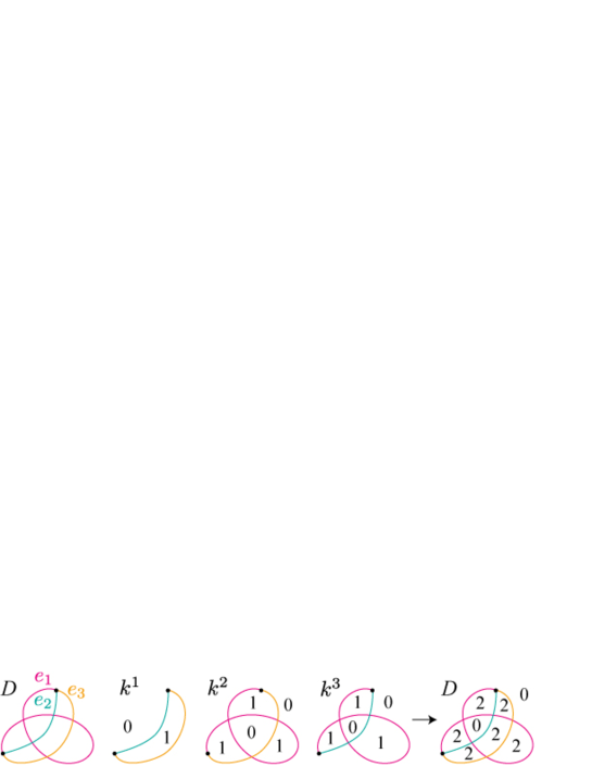
Now we show that each region of has or . Let and be regions sharing an edge . Then and take different values on both and because exists on and . And they take the same value on because and belongs to the same region on . Hence, for each pair of regions and sharing an edge, the difference between and is or . Since the outer region has , and the value of can be at most , every region has or , with the breakdown or . Therefore, is obtained by . ∎
Let be a set of regions of a reduced diagram . Let be an ineffective set for . We can obtain the same result of region crossing changes at the regions in by retaking the regions to (see [9] for knots). For a reduced diagram of a spatial -curve, by taking , and as and the above retaking, we can obtain eight sets of regions whose effects by region crossing changes are the same. We remark that , and are independent; Looking around a vertex, we can see that neither , nor can be obtained by a combination of the others. See Figure 12.

Acknowledgments
The authors thank Kota Koashi, Atsushi Oya, Hiroaki Saito, Shunta Saito and Mao Totsuka for valuable discussions in the seminars in Gunma College. They are also very grateful to Yoshiro Yaguchi for valuable discussions and helpful comments.
References
- [1] K. Ahara and M. Suzuki, An integral region choice problem on knot projection, J. Knot Theory Ramifications 21 (2012), 1250119 [20 pages].
- [2] Z. Cheng, When is region crossing change an unknotting operation?, Mathematical Proceedings of the Cambridge Philosophical Society, 155 (2013), 257–269.
- [3] Z. Cheng and H. Gao, On region crossing change and incidence matrix, Science China Mathematics 55 (2012), 1487–1495.
- [4] M. Hashizume, On the image and the cokernel of homomorphism induced by region crossing change, JP J. Geom. Topol. 18 (2015), 133–162.
- [5] K. Hayano, A. Shimizu and R. Shinjo, Region crossing change on spatial-graph diagrams, J. Knot Theory Ramifications 24 (2015), 1550045 [12 pages].
- [6] A. Inoue and R. Shimizu, A subspecies of region crossing change, region freeze crossing change, J. Knot Theory Ramifications 25 (2016), 1650075.
- [7] A. Kawauchi, On a trial of early childhood education of mathematics by a knot (in Japanese), in: Chapter one of: Introduction to Mathematical Education on Knots for primary school children, junior high students, and the high school students, No.4 (ed. A. Kawauchi and T. Yanagimoto), 2014.
- [8] A. Kawauchi, A. Shimizu and Y. Yaguchi, Cross-index of a graph, to appear in Kyungpook Math. J.
- [9] A. Shimizu, Region crossing change is an unknotting operation, J. Math. Soc. Japan 66 (2014), 693–708.