Distribution of extreme first passage times of diffusion

Abstract

Many events in biology are triggered when a diffusing searcher finds a target, which is called a first passage time (FPT). The overwhelming majority of FPT studies have analyzed the time it takes a single searcher to find a target. However, the more relevant timescale in many biological systems is the time it takes the fastest searcher(s) out of many searchers to find a target, which is called an extreme FPT. In this paper, we apply extreme value theory to find a tractable approximation for the full probability distribution of extreme FPTs of diffusion. This approximation can be easily applied in many diverse scenarios, as it depends on only a few properties of the short time behavior of the survival probability of a single FPT. We find this distribution by proving that a careful rescaling of extreme FPTs converges in distribution as the number of searchers grows. This limiting distribution is a type of Gumbel distribution and involves the LambertW function. This analysis yields new explicit formulas for approximations of statistics of extreme FPTs (mean, variance, moments, etc.) which are highly accurate and are accompanied by rigorous error estimates.

1 Introduction

Events in biological systems are often triggered when a diffusing searcher finds a target (Chou and D’Orsogna, 2014; Holcman and Schuss, 2014b; Bressloff and Newby, 2013). Examples range from the initiation of the immune response when a searching T cell finds a cognate antigen (Delgado et al., 2015), to the triggering of calcium release by diffusing IP₃ molecules that reach IP₃ receptors (Wang et al., 1995), to gene activation by the arrival of a diffusing transcription factor to a certain gene (Larson et al., 2011), to animals foraging for food (McKenzie et al., 2009; Kurella et al., 2015). In such systems, the activation timescale is determined by the first passage time (FPT) of a searcher to a target.

The vast majority of FPT studies have focused on the time it takes a given single searcher to find a target. However, several recent works and commentaries have shown that the relevant timescale in many biological systems is actually the time it takes the fastest searcher(s) to find a target out of a large group of searchers (Schuss et al., 2019; Basnayake et al., 2019b; Coombs, 2019; Redner and Meerson, 2019; Sokolov, 2019; Rusakov and Savtchenko, 2019; Martyushev, 2019; Tamm, 2019; Basnayake et al., 2018; Guerrier and Holcman, 2018). For example, approximately $N=10^{8}$ sperm cells search for an egg in human reproduction, but fertilization occurs as soon as a single sperm cell finds the egg (Meerson and Redner, 2015; Reynaud et al., 2015; Barlow, 2016; Yang et al., 2016).

Importantly, the time it takes the fastest searcher(s) out of many searchers to find a target is typically much less than the time it takes a given single searcher to find a target. In fact, Schuss et al. (2019) postulated that this is a general mechanism that operates across many biological systems and called it the redundancy principle. In particular, these authors claimed that many seemingly redundant copies of a searcher (molecule, protein, cell, animal, etc.) are not superfluous, but rather have the specific functions of accelerating activation rates. That is, the apparently “extra” copies are in fact necessary for biological function.

Indeed, the review by Schuss et al. (2019) highlights many examples of signal transduction triggered by the fastest molecules to find a target. We now explain one example recently studied by Basnayake et al. (2019a) that involves calcium-induced calcium release in dendritic spines. While the geometry can vary greatly, a dendritic spine consists roughly of a bulbous head connected to a thin neck. It has been observed that calcium ions entering at the head of the spine can diffuse to and then bind small Ryanodyne receptors at the base of the spine neck which then induces an avalanche of calcium release from internal spine apparatus stores. This calcium avalanche at the base occurs only a few milliseconds after calcium ions enter at the head, which is perplexing because the time it takes a given single calcium ion to diffuse from the head to a Ryanodyne receptor at the base is approximately $\tau=120$ milliseconds. However, through a close integration of experiments and numerical simulations, Basnayake et al. (2019a) explained this phenomenon by showing that approximately $N=10^{3}$ ions enter at the head and that the fastest ions out of this group take only a few milliseconds to reach the receptors at the base. Similar processes occur in the photoresponse of a fly to the absorption of a single photon (Katz et al., 2017; Schuss et al., 2019).

Another similar example concerns the random production of antibodies by genetic recombination inside a B cell during somatic hypermutation (Schuss et al., 2019; Coombs, 2019). In this scenario, while several gene segment copies are produced, only the first segment to find and bind a certain macromolecular complex will be used for producing antibodies. Additional examples include the IP3 pathway, in which the first IP3 molecules which find small IP3 receptors induce calcium release, and synaptic transmission, in which the pre-synaptic signal is transmitted by the first of many neurotransmitters which diffuse to and bind small post-synaptic receptors (Schuss et al., 2019).

To investigate how the number of searchers affects the time it takes the fastest searcher(s) to find a target, consider $N\gg 1$ independent and identical diffusive searchers. Let $\tau_{1},\dots,\tau_{N}$ be their independent and identically distributed (iid) FPTs to reach some target. The first time one of these searchers finds the target is

$$T_{N}:=\min\{\tau_{1},\dots,\tau_{N}\}.$$ (1)

More generally, the $k$th fastest searcher finds the target at time

$$T_{k,N}:=\min\big{\{}\{\tau_{1},\dots,\tau_{N}\}\backslash\cup_{j=1}^{k-1}\{T_{j,N}\}\big{\}},\quad k\in\{1,\dots,N\},$$ (2)

where $T_{1,N}:=T_{N}$.

The mean of a single FPT, $\mathbb{E}[\tau_{1}]$, is well understood in a variety of scenarios (Benichou et al., 2010; Cheviakov et al., 2010; Bressloff and Lawley, 2015; Lindsay et al., 2017; Lawley and Miles, 2019), and important progress has been made recently in understanding the distribution of a single FPT (Rupprecht et al., 2015; Grebenkov et al., 2018a, b, 2019). However, studying the so-called extreme FPTs, $T_{k,N}$, is notoriously difficult, both analytically and numerically (Weiss et al., 1983; Yuste and Lindenberg, 1996; Basnayake et al., 2019b; Schuss et al., 2019; Lawley and Madrid, 2020; Lawley, 2020). An essential difficulty is that extreme FPTs depend on very rare events. Indeed, while a typical searcher tends to wander around before finding the target, the fastest searchers move almost deterministically along the shortest geodesic path to the target (Godec and Metzler, 2016a, b; Grebenkov and Rupprecht, 2017; Basnayake et al., 2018; Lawley, 2020). This phenomenon is illustrated in Figure 1.

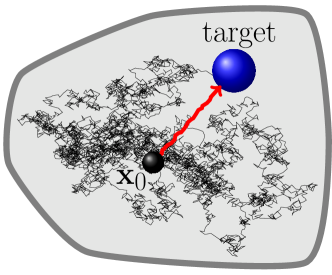
Figure 1: The fastest diffusive searcher out of $N\gg 1$ searchers moves almost deterministically (red trajectory) along the shortest path from the starting location $\mathbf{x}_{0}$ to the target (blue ball), while a typical searcher wanders around (black trajectory) before finding the target.

Another significant challenge in understanding extreme FPTs in biological applications is that the targets are often very small (Holcman and Schuss, 2014a). For example, this is the case in the application to calcium-induced calcium release in dendritic spines discussed above, as a Ryanodyne receptor can be modeled as a disk of radius $r=0.01\,\mu\text{m}$ whereas the distance from the spine head to the base of the spine neck is roughly $L=3\,\mu\text{m}$ (Basnayake et al., 2019a), and thus a dimensionless measure of the target size is

$$\varepsilon:=r/L\approx 0.003\ll 1.$$

This is a challenge because the mean fastest FPT, $\mathbb{E}[T_{N}]$, diverges for small targets ($\varepsilon\ll 1$) but vanishes for many searchers ($N\gg 1$). That is, if we fix the number of searchers $N$ and take the target size $\varepsilon$ sufficiently small, then

$$\tfrac{D}{L^{2}}\mathbb{E}[T_{N}]\gg 1,$$ (3)

where $\tfrac{L^{2}}{D}$ is the diffusion timescale. On the other hand, if we fix the target size $\varepsilon$ and take the number of searchers $N$ sufficiently large, then

$$\tfrac{D}{L^{2}}\mathbb{E}[T_{N}]\ll 1.$$ (4)

Hence, as a first step in any specific biological application involving extreme FPTs with small targets ($\varepsilon\ll 1$) and many searchers ($N\gg 1$), one needs to determine if the extreme FPTs are in the regime represented by either (3) or (4). For example, in the dendritic spine application described above, it is not a priori clear that $N=10^{3}$ is sufficiently large to overcome the small Ryanodyne receptors ($\varepsilon\approx 0.003$) and make the extreme FPT on the order of only 2-3 milliseconds (which is much less than the diffusion timescale in this problem, $\tfrac{L^{2}}{D}\approx 15$ milliseconds). Indeed, Basnayake et al. (2019a) developed detailed numerical Monte Carlo simulations to reach this conclusion.

Importantly, analytical approximations of statistics of extreme FPTs for small targets in general 3-dimensional domains are lacking. Basnayake et al. (2019b) derived a formal approximation, but this was proven to be false (Lawley and Madrid, 2020). Recent work found the leading order large $N$ behavior of all the moments of $T_{k,N}$, but it turns out this leading order behavior is independent of the target size (Lawley, 2020). Hence, these results cannot determine if a particular application is in the regime represented by (3) or (4).

In this paper, we apply the theory of extreme statistics to find a tractable approximation for the full probability distribution of extreme FPTs of diffusion. This rigorous approximation can be applied in many scenarios as it depends on only a few properties of the short time behavior of the survival probability of a single FPT. Indeed, as long as this short time behavior is known, this approximation can be immediately applied to scenarios involving small targets and thus can determine the influence of the competing limits of small targets ($\varepsilon\ll 1$) and many searchers ($N\gg 1$).

We find this distribution by proving that a careful rescaling of extreme FPTs converges in distribution as the number of searchers grows. This limiting distribution is a type of Gumbel distribution and involves the so-called LambertW function (defined as the inverse of $f(z)=ze^{z}$ (Corless et al., 1996)). This analysis yields new explicit formulas for statistics of extreme FPTs (mean, variance, moments, etc.). These formulas are highly accurate and are accompanied by rigorous error estimates. Further, these formulas confirm and explain a conjecture by Yuste et al. (2001) that extreme FPT statistics can be approximated by a certain infinite series involving iterated logarithms.

The rest of the paper is organized as follows. We first summarize our main results in section 2. In section 3, we develop and state our precise mathematical results in more detail. We then illustrate these general results in a few examples in section 4. In the Discussion section, we describe relations to prior work and discuss applications of the theory. Finally, we collect all the mathematical proofs in an appendix.

2 Main results

Let $\{\tau_{n}\}_{n\geq 1}$ be an iid sequence of FPTs with survival probability

$$S(t):=\mathbb{P}(\tau_{1}>t).$$

Assume that $S(t)$ has the short time behavior,

$$1-S(t)\sim At^{p}e^{-C/t}\quad\text{as }t\to 0+,$$ (5)

for some constants $A>0$, $C>0$, and $p\in\mathbb{R}$. Throughout this work,

$$\text{``$f\sim g$'' means }f/g\to 1.$$

We emphasize that (5) is a generic behavior for diffusion processes that holds in many diverse scenarios (see the Discussion section for more details).

Letting $T_{N}$ denote the fastest FPT in (1), we prove the following convergence in distribution (Theorem 3.1),

$$\frac{T_{N}-b_{N}}{a_{N}}\to_{\textup{d}}X\quad\text{as }N\to\infty,$$ (6)

where $X$ has a standard Gumbel distribution, $\mathbb{P}(X>x)=\exp(-e^{x})$, and

$$\begin{split}a_{N}&=\frac{b_{N}}{\ln(AN)},\quad b_{N}=\frac{C}{\ln(AN)},\quad\text{if }p=0,\\ a_{N}&=\frac{b_{N}}{p(1+W)},\quad b_{N}=\frac{C}{pW},\quad\text{if }p\neq 0,\end{split}$$ (7)

and

$$W =\begin{cases}W_{0}\big{(}(C/p)(AN)^{1/p}\big{)}&\text{if }p>0,\\ W_{-1}\big{(}(C/p)(AN)^{1/p}\big{)}&\text{if }p<0,\end{cases}$$

where $W_{0}(z)$ denotes the principal branch of the LambertW function and $W_{-1}(z)$ denotes the lower branch (Corless et al., 1996). The LambertW function is a fairly standard function that is included in most modern computational software (it is sometimes called the product logarithm or the omega function). Theorem 3.2 gives the following alternative formulas for $a_{N}$ and $b_{N}$ which avoid the LambertW function,

$$a_{N}^{\prime} =\frac{C}{(\ln N)^{2}},\quad b_{N}^{\prime}=\frac{C}{\ln N}+\frac{Cp\ln(\ln(N))}{(\ln N)^{2}}-\frac{C\ln(AC^{p})}{(\ln N)^{2}}.$$ (8)

In particular, all the statements in this section hold with $a_{N},b_{N}$ replaced by $a_{N}^{\prime},b_{N}^{\prime}$.

The convergence in distribution in (6) means that if $N\gg 1$, then the distribution of the fastest FPT, $T_{N}$, is approximately Gumbel with shape parameter $b_{N}$ and scale parameter $a_{N}$. That is,

$$\mathbb{P}(T_{N}>t)\approx\exp\Big{[}-\exp\Big{(}\frac{t-b_{N}}{a_{N}}\Big{)}\Big{]}\quad\text{if }N\gg 1,$$

where $a_{N},b_{N}$ are in (7) (or are replaced by $a_{N}^{\prime},b_{N}^{\prime}$ in (8)). Note that essentially all the statistical information about a Gumbel distribution is immediately available (mean, median, mode, variance, moments, probability density function, etc., see Proposition 1 below). Therefore, this result provides all the statistical information for the fastest FPT (approximately for large $N$). For example, we prove that if $\mathbb{E}[T_{N}]<\infty$ for some $N\geq 1$, then (Theorem 3.3)

$$\mathbb{E}[T_{N}] =b_{N}-\gamma a_{N}+o(a_{N}),$$

$$\textup{Variance}(T_{N}) =\frac{\pi^{2}}{6}a_{N}^{2}+o(a_{N}^{2}),$$

where $\gamma\approx 0.5772$ is the Euler-Mascheroni constant and $f(N)=o(a_{N}^{m})$ means $\lim_{N\to\infty}a_{N}^{-m}f(N)=0$.

We prove similar results for the $k$th fastest FPT, $T_{k,N}$, defined in (2). In particular, we prove that the joint distribution of a rescaling of the $k$ fastest FPTs,

$$\left(\frac{T_{1,N}-b_{N}}{a_{N}},\dots,\frac{T_{k,N}-b_{N}}{a_{N}}\right),$$

converges as $N\to\infty$ to a distribution that we give explicitly (Theorem 3.4). This result provides explicit approximations for statistics of $T_{k,N}$, including (Theorem 3.5),

$$\mathbb{E}[T_{k,N}] =b_{N}+\psi(k)a_{N}+o(a_{N})=\mathbb{E}[T_{N}]+H_{k-1}a_{N}+o(a_{N}),$$

$$\textup{Variance}(T_{k,N}) =\psi^{\prime}(k)a_{N}^{2}+o(a_{N}^{2}),$$

where $\psi(x)$ is the digamma function and $H_{k-1}=\sum_{r=1}^{k-1}\tfrac{1}{r}$ is the $(k-1)$-th harmonic number.

3 Mathematical analysis

3.1 Fastest FPT

Let $\{\tau_{n}\}_{n\geq 1}$ be an iid sequence of FPTs with survival probability $S(t):=\mathbb{P}(\tau_{1}>t)$. Define the fastest FPT, $T_{N}$, as in (1). Since the sequence $\{\tau_{n}\}_{n\geq 1}$ is iid, it is immediate that the survival probability of $T_{N}$ is

$$\mathbb{P}(T_{N}>t)=(\mathbb{P}(\tau_{1}>t))^{N}=(S(t))^{N}.$$ (9)

While (9) is the exact distribution of $T_{N}$, this formula it is not particularly useful for understanding how the distribution depends on parameters or for calculating statistics of $T_{N}$. Furthermore, the full survival probability $S(t)$ of a single FPT is often unknown.

We thus seek a tractable approximation of (9) for large $N$, which will thus depend only on the short time behavior of $S(t)$. Now, (9) implies that the limiting distribution of $T_{N}$ for large $N$ is trivial,

$$\lim_{N\to\infty}\mathbb{P}(T_{N}>t)=\begin{cases}1&\text{if }t<t^{*},\\ 0&\text{if }t>t^{*},\end{cases}$$

where $t^{*}:=\inf\{t>0:S(t)<1\}$. For nontrivial diffusion processes, we typically have $t^{*}=0$. To ameliorate this problem, we study the distribution of $T_{N}$ by finding a rescaling of $T_{N}$ that has a nontrivial limiting distribution for large $N$. Specifically, we find sequences $\{a_{N}\}_{N\geq 1}$ and $\{b_{N}\}_{N\geq 1}$ so that

$$\frac{T_{N}-b_{N}}{a_{N}}\to_{\textup{d}}X\quad\text{as }N\to\infty,$$

for some random variable $X$. In this paper, $\to_{\textup{d}}$ denotes convergence in distribution (Billingsley, 2013), which means

$$\mathbb{P}\left(\frac{T_{N}-b_{N}}{a_{N}}>x\right)=(S(a_{N}x+b_{N}))^{N}\to G(x)\quad\text{as }N\to\infty,$$ (10)

for all $x\in\mathbb{R}$ where $G(x)=\mathbb{P}(X>x)$ is continuous.

Remarkably, the Fisher-Tippett-Gnedenko Theorem states that if (10) holds for a nondegenerate $G$, then $G$ must be either a Weibull, Frechet, or Gumbel distribution (Fisher and Tippett, 1928). This theorem is the cornerstone of extreme value theory, and applies to the minimum or maximum of any sequence of iid random variables (Coles, 2001; De Haan and Ferreira, 2007; Falk et al., 2010). Since the limiting distribution must be one of these three types, this classical theorem is an extreme value analog of the central limit theorem. We prove below that the typical short time behavior of $S(t)$ ensures that $G$ must be Gumbel. The following definition and proposition collects some facts about the Gumbel distribution.

Definition 1.

A random variable $X$ has a Gumbel distribution with location parameter $b\in\mathbb{R}$ and scale parameter $a>0$ if

$$\mathbb{P}(X>x)=\exp\Big{[}-\exp\Big{(}\frac{x-b}{a}\Big{)}\Big{]},\quad\text{for all }x\in\mathbb{R}.$$ (11)

If (11) holds, then we write

$$X=_{\textup{d}}\textup{Gumbel}(b,a).$$

Proposition 1.

If $X=_{\textup{d}}\textup{Gumbel}(b,a)$, then its survival probability is in (11), its probability density function is

$$f_{X}(x)=\frac{1}{a}\exp\Big{[}\frac{x-b}{a}-\exp\Big{(}\frac{x-b}{a}\Big{)}\Big{]},\quad x\in\mathbb{R},$$

and its moment generating function is

$$M_{X}(t):=\mathbb{E}[e^{tX}]=\Gamma(1+at)e^{bt},\quad t\in\mathbb{R},$$

where $\Gamma(\cdot)$ denotes the gamma function. Hence, the mean and variance are

$$\mathbb{E}[X]=b-\gamma a,\quad\textup{Variance}(X)=\frac{\pi^{2}}{6}a^{2},$$

where $\gamma\approx 0.5772$ is the Euler-Mascheroni constant. The mode and median are

$$\textup{Mode}(X)=b,\quad\textup{Median}(X)=b+a\ln(\ln(2))\approx b-0.3665a.$$

Now, it was recently proven that under very general assumptions, the survival probability of a single diffusive FPT has the following short time behavior,

$$\lim_{t\to 0+}t\ln(1-S(t))=-C<0,$$ (12)

where $C=L^{2}/(4D)>0$ and $D$ is a characteristic diffusivity and $L$ is a certain geodesic distance (Lawley, 2020), as long as the diffusive searchers cannot start arbitrarily close to the target. The next proposition shows that if (12) holds, then any nondegenerate limiting distribution $G$ in (10) must be Gumbel.

Proposition 2.

Let $\{\tau_{n}\}_{n\geq 1}$ be an iid sequence of nonnegative random variables with $S(t):=\mathbb{P}(\tau_{1}>t)$, define $T_{N}:=\min\{\tau_{1},\dots,\tau_{N}\}$, and suppose (12) holds. If there exists sequences $\{a_{N}\}_{N\geq 1}$ and $\{b_{N}\}_{N\geq 1}$ with $a_{N}>0$ and $b_{N}\in\mathbb{R}$ so that

$$\frac{T_{N}-b_{N}}{a_{N}}\to_{\textup{d}}X\quad\text{as }N\to\infty,$$

and $X$ has a nondegenerate distribution, then $X=_{\textup{d}}\textup{Gumbel}(b,a)$ for some $b\in\mathbb{R}$ and $a>0$.

The condition in (12) implies that

$$S(t)=1-e^{-C/t+h(t)},$$

where $h(t)$ is some function satisfying $th(t)\to 0$ as $t\to 0+$. The following proposition gives precise conditions on $h(t)$ which yield rescalings $\{a_{N}\}_{N\geq 1}$ and $\{b_{N}\}_{N\geq 1}$ so that $(T_{N}-b_{N})/a_{N}$ converges in distribution to a Gumbel random variable.

Proposition 3.

Let $\{\tau_{n}\}_{n\geq 1}$ be an iid sequence of nonnegative random variables with $S(t):=\mathbb{P}(\tau_{1}>t)$, define $T_{N}:=\min\{\tau_{1},\dots,\tau_{N}\}$, and assume

$$1-S(t)\sim 1-S_{0}(t)\quad\text{as }t\to 0+,$$

where

$$S_{0}(t)=1-e^{-C/t+h(t)},\quad\text{if }t>0,$$

for some constant $C>0$ and some function $h(t)$ that is twice-continuously differentiable for $t>0$ and satisfies

$$\lim_{t\to 0+}th(t)=\lim_{t\to 0+}t^{2}h^{\prime}(t)=\lim_{t\to 0+}t^{4}h^{\prime\prime}(t)=0.$$ (13)

Then

$$\frac{T_{N}-b_{N}}{a_{N}}\to_{\textup{d}}X=_{\textup{d}}\textup{Gumbel}(0,1)\quad\text{as }N\to\infty,$$

where

$$a_{N} :=\frac{-1}{NS_{0}^{\prime}(b_{N})}>0,\quad b_{N}:=S_{0}^{-1}(1-1/N)>0,\quad N\geq 1.$$ (14)

In (14), $S_{0}^{-1}(1-1/N)$ denotes the inverse of $S_{0}$, which must exist for large $N$ by the assumptions on $h(t)$. As we will see, it is typically the case that $h(t)=\ln(At^{p})$, which clearly satisfies (13). In this case, we work out the rescalings $\{a_{N}\}_{N\geq 1}$ and $\{b_{N}\}_{N\geq 1}$.

Theorem 3.1.

Let $\{\tau_{n}\}_{n\geq 1}$ be an iid sequence of nonnegative random variables with $S(t):=\mathbb{P}(\tau_{1}>t)$, define $T_{N}:=\min\{\tau_{1},\dots,\tau_{N}\}$, and assume there exists constants $C>0$, $A>0$, and $p\in\mathbb{R}$ so that

$$1-S(t)\sim At^{p}e^{-C/t}\quad\text{as }t\to 0+.$$

Then

$$\frac{T_{N}-b_{N}}{a_{N}}\to_{\textup{d}}X=_{\textup{d}}\textup{Gumbel}(0,1)\quad\text{as }N\to\infty,$$ (15)

where

$$\begin{split}a_{N}&=\frac{b_{N}}{\ln(AN)},\quad b_{N}=\frac{C}{\ln(AN)},\quad\text{if }p=0,\\ a_{N}&=\frac{b_{N}}{p(1+W)},\quad b_{N}=\frac{C}{pW},\quad\text{if }p\neq 0,\end{split}$$ (16)

and

$$W =\begin{cases}W_{0}\big{(}(C/p)(AN)^{1/p}\big{)}&\text{if }p>0,\\ W_{-1}\big{(}(C/p)(AN)^{1/p}\big{)}&\text{if }p<0,\end{cases}$$ (17)

where $W_{0}(z)$ denotes the principal branch of the LambertW function and $W_{-1}(z)$ denotes the lower branch (Corless et al., 1996).

If the convergence in distribution in (15) holds for some rescalings $\{a_{N}\}_{N\geq 1}$ and $\{b_{N}\}_{N\geq 1}$, then we also have that

$$\frac{T_{N}-b_{N}^{\prime}}{a_{N}^{\prime}}\to_{\textup{d}}X=_{\textup{d}}\textup{Gumbel}(0,1)\quad\text{as }N\to\infty,$$ (18)

for any rescalings $\{a_{N}^{\prime}\}_{N\geq 1}$ and $\{b_{N}^{\prime}\}_{N\geq 1}$ that satisfy (Peng and Nadarajah, 2012)

$$\lim_{N\to\infty}\frac{a_{N}^{\prime}}{a_{N}}=1,\quad\lim_{N\to\infty}\frac{b_{N}^{\prime}-b_{N}}{a_{N}}=0.$$ (19)

The following theorem gives rescalings which avoid the LambertW functions used in Theorem 3.1 and are valid for any $p\in\mathbb{R}$.

Theorem 3.2.

Under the assumptions of Theorem 3.1, we have that

$$\frac{T_{N}-b_{N}^{\prime}}{a_{N}^{\prime}}\to_{\textup{d}}X=_{\textup{d}}\textup{Gumbel}(0,1)\quad\text{as }N\to\infty,$$

where

$$\begin{split}a_{N}^{\prime}&=\frac{C}{(\ln N)^{2}},\quad b_{N}^{\prime}=\frac{C}{\ln N}+\frac{Cp\ln(\ln(N))}{(\ln N)^{2}}-\frac{C\ln(AC^{p})}{(\ln N)^{2}}.\end{split}$$ (20)

The conclusions of Propositions 2-3 and Theorems 3.1-3.2 concern convergence in distribution. In general, convergence in distribution does not imply moment convergence (Billingsley, 2013). That is, $X_{N}\to_{\textup{d}}X$ does not necessarily imply $\mathbb{E}[(X_{N})^{m}]\to\mathbb{E}[X^{m}]$ for $m>0$. However, Pickands (1968) proved that convergence in distribution does imply moment convergence for extreme values.

Theorem 3.3.

Under the assumptions of Theorem 3.1 with $\{a_{N}\}_{N\geq 1}$ and $\{b_{N}\}_{N\geq 1}$ given by either (16) or (20), assume further that $\mathbb{E}[T_{N}]<\infty$ for some $N\geq 1$. Then for each moment $m\in(0,\infty)$, we have that

$$\mathbb{E}\left[\left(\frac{T_{N}-b_{N}}{a_{N}}\right)^{m}\right]\to\mathbb{E}[X^{m}]\quad\text{as }N\to\infty,\quad\text{where }X=_{\textup{d}}\textup{Gumbel}(0,1).$$

Therefore,

$$\mathbb{E}[(T_{N}-b_{N})^{m}]=a_{N}^{m}\mathbb{E}[X^{m}]+o(a_{N}^{m}),$$

where $f(N)=o(a_{N}^{m})$ means $\lim_{N\to\infty}a_{N}^{-m}f(N)=0$. Further, if $m>0$ is an integer, then $\mathbb{E}[X^{m}]$ can be calculated explicitly by Proposition 1. For example, we have that

$$\mathbb{E}[T_{N}] =b_{N}-\gamma a_{N}+o(a_{N}),$$

$$\textup{Variance}(T_{N}) =\frac{\pi^{2}}{6}a_{N}^{2}+o(a_{N}^{2}),$$

where $\gamma\approx 0.5772$ is the Euler-Mascheroni constant.

3.2 $k$th fastest FPT

We now extend the results in the previous subsection on the fastest FPT to the $k$th fastest FPT,

$$T_{k,N}:=\min\big{\{}\{\tau_{1},\dots,\tau_{N}\}\backslash\cup_{j=1}^{k-1}\{T_{j,N}\}\big{\}},\quad k\in\{1,\dots,N\},$$

where $T_{1,N}:=T_{N}$.

Theorem 3.4.

Under the assumptions of Theorem 3.1 with $\{a_{N}\}_{N\geq 1}$ and $\{b_{N}\}_{N\geq 1}$ given by either (16) or (20), we have that for each fixed $k\geq 1$,

$$\frac{T_{k,N}-b_{N}}{a_{N}}\to_{\textup{d}}X_{k}\quad\text{as }N\to\infty,$$ (21)

where $X_{k}$ has the probability density function,

$$f_{X_{k}}(x)=\frac{\exp(kx-e^{x})}{(k-1)!},\quad\text{for all }x\in\mathbb{R}.$$ (22)

Furthermore, for each fixed $k\geq 1$, we have the following convergence in distribution for the joint random variables,

$$\left(\frac{T_{1,N}-b_{N}}{a_{N}},\dots,\frac{T_{k,N}-b_{N}}{a_{N}}\right)\to_{\textup{d}}\mathbf{X}^{(k)}=(X_{1},\dots,X_{k})\in\mathbb{R}^{k}\quad\text{as }N\to\infty,$$ (23)

where the joint probability density function of $\mathbf{X}^{(k)}\in\mathbb{R}^{k}$ is

$$f_{\mathbf{X}^{(k)}}(x_{1},\dots,x_{k}) =\begin{cases}\exp(-e^{x_{k}})\prod_{r=1}^{k}e^{x_{r}}&\text{if $x_{1}\leq\dots\leq x_{k}$},\\ 0&\text{otherwise}.\end{cases}$$

The following theorem ensures the convergence of the moments of the $k$th fastest FPT.

Theorem 3.5.

Under the assumptions of Theorem 3.3 with $\{a_{N}\}_{N\geq 1}$ and $\{b_{N}\}_{N\geq 1}$ given by either (16) or (20), we have that for each moment $m\in(0,\infty)$,

$$\mathbb{E}\left[\left(\frac{T_{k,N}-b_{N}}{a_{N}}\right)^{m}\right]\to\mathbb{E}[X_{k}^{m}]\quad\text{as }N\to\infty,$$ (24)

where $X_{k}$ has the probability density function in (22). Therefore,

$$\mathbb{E}[(T_{k,N}-b_{N})^{m}]=a_{N}^{m}\mathbb{E}[X_{k}^{m}]+o(a_{N}^{m}).$$

Further, if $m>0$ is an integer, then $\mathbb{E}[X_{k}^{m}]$ can be explicitly calculated. In particular,

$$\mathbb{E}[T_{k,N}] =b_{N}+\psi(k)a_{N}+o(a_{N})=\mathbb{E}[T_{1,N}]+H_{k-1}a_{N}+o(a_{N}),$$

$$\textup{Variance}(T_{k,N}) =\psi^{\prime}(k)a_{N}^{2}+o(a_{N}^{2}),$$

where $\psi(x)$ is the digamma function and $H_{k-1}=\sum_{r=1}^{k-1}\tfrac{1}{r}$ is the $(k-1)$-th harmonic number.

4 Numerical examples

We now apply our results to three specific examples.

4.1 One dimension

First consider the case of $N\geq 1$ independent searchers diffusing in one space dimension with diffusivity $D>0$. Suppose the searchers each start at ${L}>0$ and let $\tau_{n}$ be the first time the $n$th searcher reaches the origin. In this case,

$$S(t)=\mathbb{P}(\tau_{1}>t)=1-\text{erfc}\Big{(}\frac{{{L}}}{\sqrt{4Dt}}\Big{)},\quad t>0,$$

and thus

$$1-S(t)\sim\sqrt{\frac{4Dt}{\pi{L}^{2}}}e^{-{L}^{2}/(4Dt)}\quad\text{as }t\to 0+.$$

Therefore, Theorems 3.1-3.5 hold with

$$A=\sqrt{\frac{4D}{\pi{L}^{2}}},\quad p=\frac{1}{2},\quad C=\frac{{L}^{2}}{4D}.$$

In particular,

$$\frac{T_{N}-b_{N}}{a_{N}}\to_{\textup{d}}X=_{\textup{d}}\textup{Gumbel}(0,1)\quad\text{as }N\to\infty,$$

where $\{a_{N}\}_{N\geq 1}$ and $\{b_{N}\}_{N\geq 1}$ are given by either (16) or (20). Hence, the distribution of $T_{N}$ is approximately $\textup{Gumbel}(b_{N},a_{N})$.

In the left panel of Figure 2, we plot the error of various approximations of the mean fastest FPT, $\mathbb{E}[T_{N}]$, as functions of $N$. Specifically, we plot the relative error,

$$\Big{|}\frac{\mathbb{E}[T_{N}]-\mathcal{T}_{N}}{\mathbb{E}[T_{N}]}\Big{|},$$ (25)

where $\mathcal{T}_{N}$ is an approximation of $\mathbb{E}[T_{N}]$. The value of $\mathbb{E}[T_{N}]$ used in (25) is calculated by numerical approximation of the following integral,

$$\mathbb{E}[T_{N}]=\int_{0}^{\infty}(S(t))^{N}\,\text{d}t.$$

The red dotted curve in the left panel of Figure 2 is the error (25) for the approximation $\mathcal{T}_{N}=L^{2}/(4D\ln N)$ (this approximation dates back to Weiss et al. (1983)). The blue dashed curve is for the approximation $\mathcal{T}_{N}=b_{N}^{\prime}-\gamma a_{N}^{\prime}$ where $\{a_{N}^{\prime}\}_{N\geq 1}$ and $\{b_{N}^{\prime}\}_{N\geq 1}$ are given by (20). The black solid curve is for the approximation $\mathcal{T}_{N}=b_{N}-\gamma a_{N}$ where $\{a_{N}\}_{N\geq 1}$ and $\{b_{N}\}_{N\geq 1}$ are given by (16). This figure shows that our approximations, $b_{N}-\gamma a_{N}$ and $b_{N}^{\prime}-\gamma a_{N}^{\prime}$, to the mean fastest FPT are much more accurate than $L^{2}/(4D\ln N)$, and $b_{N}-\gamma a_{N}$ is more accurate than $b_{N}^{\prime}-\gamma a_{N}^{\prime}$.

In the left panel of Figure 3, we illustrate the convergence in distribution of $(T_{N}-b_{N})/a_{N}$ to $X=_{\textup{d}}\textup{Gumbel}(0,1)$ where $\{a_{N}\}_{N\geq 1}$ and $\{b_{N}\}_{N\geq 1}$ are given by (16). Specifically, we plot the probability density function of $(T_{N}-b_{N})/a_{N}$ for $N\in\{10^{2},10^{4},10^{6}\}$, which approaches the density of $X$ (namely, $f_{X}(x)=\exp(x-e^{x})$) as $N$ increases. In both Figures 2 and 3, we take $L=D=1$.

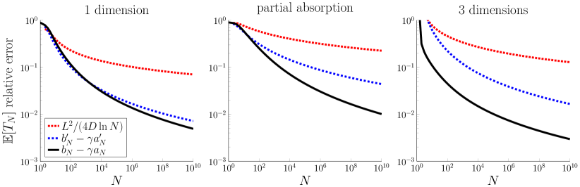
Figure 2: Accuracy of approximations to the mean fastest FPT. The left, middle, and right panels correspond respectively to the examples in sections 4.1, 4.2, and 4.3. In each panel, the red dotted curve is the relative error (25) for the approximation $L^{2}/(4D\ln N)$, the blue dashed curve is for $b_{N}^{\prime}-\gamma a_{N}^{\prime}$ where $a_{N}^{\prime},b_{N}^{\prime}$ are given by (20), and the black solid curve is for $b_{N}-\gamma a_{N}$ where $a_{N},b_{N}$ are given by (16).

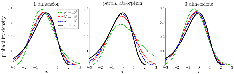
Figure 3: Convergence in distribution of rescaled fastest FPT. The left, middle, and right panels correspond respectively to the examples in sections 4.1, 4.2, and 4.3. In each panel, the green dashed, red dotted, and blue dashed-dotted curves give the probability density function of $(T_{N}-b_{N})/a_{N}$ for $N\in\{10^{2},10^{4},10^{6}\}$ where $\{a_{N}\}_{N\geq 1}$ and $\{b_{N}\}_{N\geq 1}$ are given by (16), and the black solid curve shows the limiting probability density function, $\exp(x-e^{x})$.

4.2 Partial absorption

Consider the example in the previous subsection, but now suppose the target at the origin is partially absorbing. This means that when a searcher hits the target, it is either absorbed or reflected, and the probabilities of these two events are described by a parameter $\kappa>0$ called the reactivity or absorption rate (Grebenkov, 2006). Mathematically, this means the Fokker-Planck equation describing the probability density for a searcher’s position has a Robin boundary condition at the origin involving the parameter $\kappa>0$ (Lawley and Keener, 2015).

In this case, the survival probability for a single searcher is (Carslaw and Jaeger, 1959)

$$S(t)=\mathbb{P}(\tau_{1}>t)=1-\text{erfc}\Big{(}\frac{{{L}}}{\sqrt{4Dt}}\Big{)}+e^{\frac{\kappa(\kappa t+{{L}})}{D}}\text{erfc}\Big{(}\frac{2\kappa t+{{L}}}{\sqrt{4Dt}}\Big{)},\quad t>0,$$

and thus

$$1-S(t)\sim\frac{4}{\sqrt{\pi}}\frac{\kappa{L}}{D}\Big{(}\frac{Dt}{{L}^{2}}\Big{)}^{3/2}e^{-{L}^{2}/(4Dt)}\quad\text{as }t\to 0+.$$

Therefore, Theorems 3.1-3.5 hold with

$$A=\frac{4}{\sqrt{\pi}}\frac{\kappa{L}}{D}\Big{(}\frac{D}{{L}^{2}}\Big{)}^{3/2},\quad p=\frac{3}{2},\quad C=\frac{{L}^{2}}{4D}.$$ (26)

The middle panel of Figure 2 shows the relative error (25) of approximations to $\mathbb{E}[T_{N}]$ in this case of a partially absorbing target. The red dotted curve is again the error for the approximation $\mathcal{T}_{N}=L^{2}/(4D\ln N)$ (this approximation was recently found and proven to have the correct large $N$ asymptotics (Lawley, 2020)). The blue dashed and black solid curves again correspond respectively to $\mathcal{T}_{N}=b_{N}^{\prime}-\gamma a_{N}^{\prime}$ and $\mathcal{T}_{N}=b_{N}-\gamma a_{N}$ where $a_{N}^{\prime},b_{N}^{\prime}$ are in (20) and $a_{N},b_{N}$ are in (16). Again, $b_{N}-\gamma a_{N}$ and $b_{N}^{\prime}-\gamma a_{N}^{\prime}$ are much more accurate than $L^{2}/(4D\ln N)$, and $b_{N}-\gamma a_{N}$ is more accurate than $b_{N}^{\prime}-\gamma a_{N}^{\prime}$.

The middle panel of Figure 3 illustrates the convergence in distribution of $(T_{N}-b_{N})/a_{N}$ to $X=_{\textup{d}}\textup{Gumbel}(0,1)$ in this case of a partially absorbing target (again, for $N\in\{10^{2},10^{4},10^{6}\}$ and where $\{a_{N}\}_{N\geq 1}$ and $\{b_{N}\}_{N\geq 1}$ are given by (16)). In both Figures 2 and 3, we take $L=D=\kappa=1$.

4.3 Three dimensions

Finally, consider the case where the $N\geq 1$ independent searchers diffuse in three dimensional space, and let $\tau_{n}$ be the first time the $n$th searcher leaves a sphere of radius $L>0$ centered at its starting location. In this case, the survival probability for a single searcher is (Carslaw and Jaeger, 1959)

$$S(t)=\mathbb{P}(\tau_{1}>t)=1-2\sqrt{\frac{L^{2}}{\pi Dt}}\sum_{j=0}^{\infty}e^{-(j+1/2)^{2}L^{2}/(Dt)},\quad t>0,$$

and thus

$$1-S(t)\sim 2\sqrt{\frac{L^{2}}{\pi Dt}}e^{-L^{2}/(4Dt)}\quad\text{as }t\to 0+.$$

Therefore, Theorems 3.1-3.5 hold with

$$A=2\sqrt{\frac{L^{2}}{\pi D}},\quad p=-\frac{1}{2},\quad C=\frac{{L}^{2}}{4D}.$$

The right panel of Figure 2 shows the relative error (25) of approximations to $\mathbb{E}[T_{N}]$ in this three dimensional example. The red dotted curve is again the error for the approximation $\mathcal{T}_{N}=L^{2}/(4D\ln N)$ (this approximation was found by Yuste et al. (2001)). The blue dashed and black solid curves again correspond respectively to $\mathcal{T}_{N}=b_{N}^{\prime}-\gamma a_{N}^{\prime}$ and $\mathcal{T}_{N}=b_{N}-\gamma a_{N}$ where $a_{N}^{\prime},b_{N}^{\prime}$ are in (20) and $a_{N},b_{N}$ are in (16). Further, the right panel of Figure 3 illustrates the convergence in distribution of $(T_{N}-b_{N})/a_{N}$ to $X=_{\textup{d}}\textup{Gumbel}(0,1)$ in this three dimensional example (again, for $N\in\{10^{2},10^{4},10^{6}\}$ and where $\{a_{N}\}_{N\geq 1}$ and $\{b_{N}\}_{N\geq 1}$ are given by (16)). In both Figures 2 and 3, we take $L=D=1$.

5 Discussion

In this work, we found tractable approximations for the full probability distribution of extreme FPTs of diffusion. These approximate distributions depend on only three parameters describing the short time behavior of the survival probability of a single searcher, and we proved that these approximations are exact in the many searcher limit. We used our approximate distributions to derive new formulas for statistics of extreme FPTs and prove rigorous error estimates.

Extreme FPTs of diffusion were first studied by Weiss, Shuler, and Lindenberg (1983), where they found approximations of $\mathbb{E}[T_{k,N}]$ for large $N$ in various one dimensional problems. Statistics of extreme FPTs of diffusion in one dimensional or spherically symmetric domains were further studied by Yuste and Lindenberg (1996), Yuste and Acedo (2000), Yuste et al. (2001), van Beijeren (2003), Redner and Meerson (2014), and Meerson and Redner (2015). Recently, approximate formulas for the moments of extreme FPTs of diffusion in more general two and three dimensional domains were derived by Ro and Kim (2017), Basnayake et al. (2019b), and Lawley and Madrid (2020). Even more recently, it was proven in significant generality that the $m$th moment of the $k$th fastest FPT has the large $N$ behavior,

$$\mathbb{E}[(T_{k,N})^{m}]\sim\Big{(}\frac{L^{2}}{4D\ln N}\Big{)}^{m}\quad\text{as }N\to\infty,$$ (27)

where $D$ is a characteristic diffusivity and $L$ is a certain geodesic distance (Lawley, 2020).

The moment formulas derived in the present work agree with (27) to leading order, but are much more accurate for finite $N$. In addition, the moment formulas in the present work explain and confirm a remarkable conjecture by Yuste and Acedo (2000). In that work, the authors conjectured that the mean fastest FPT to escape a ball of radius $L$ in dimension $d\geq 2$ has the following approximation,

$$\mathbb{E}[T_{1,N}]\approx\frac{L^{2}}{4D\ln N}\Big{[}1+\sum_{n=1}^{\infty}(\ln N)^{-n}\sum_{m=0}^{n}K_{m}^{(n)}(\ln\ln N)^{m}\Big{]},$$ (28)

for some unknown constants $\{\{K_{m}^{(n)}\}_{m=0}^{n}\}_{n\geq 1}$ (some of which were estimated numerically). To derive (28) from our results, first note that the principal branch of the LambertW function has the following expansion for $z\gg 1$ (Corless et al., 1996),

$$\begin{split}W_{0}(z)&=L_{1}-L_{2}+\sum_{i=0}^{\infty}\sum_{j=1}^{\infty}c_{ij}L_{1}^{-i-j}L_{2}^{j},\end{split}$$ (29)

where $L_{1}=\ln z$, $L_{2}=\ln\ln z$,

$$c_{ij}=\frac{(-1)^{i}}{j!}\left[\begin{matrix}i+j\\ i+1\end{matrix}\right],$$

and $\left[\begin{smallmatrix}i+j\\ i+1\end{smallmatrix}\right]$ are non-negative Stirling numbers of the first kind. Similarly, the lower branch, $W_{-1}(z)$, has the expansion in (29) for $-1\ll z<0$ if $L_{1}=\ln(-z)$ and $L_{2}=\ln(-\ln(-z))$ (Corless et al., 1996). Therefore, upon using the definitions in (16)-(17) and the expansion in (29), it follows that our formula $\mathbb{E}[T_{1,N}]\approx b_{N}-\gamma a_{N}$ is exactly of the form in the conjecture (28).

Finally, we emphasize that our results apply to any FPT problem where the survival probability $S(t)=\mathbb{P}(\tau_{1}>t)$ of a single searcher satisfies

$$1-S(t)\sim At^{p}e^{-C/t}\quad\text{as }t\to 0+,$$ (30)

for some constants $C>0$, $A>0$, and $p\in\mathbb{R}$. The behavior in (30) is very generic for diffusion processes and holds in many diverse scenarios. For example, Weiss et al. (1983) found (30) for one-dimensional drift-diffusion processes with a broad class of potential (drift) fields. Similarly, Yuste et al. (2001) found (30) for the first time a pure diffusion in dimension $d\geq 1$ moves any distance $L>0$ from its initial location (and referred to (30) as a “universal” form). Further, Ro and Kim (2017) formally derived (30) for a pure diffusion searching for an arbitrarily placed small target in a spherical domain in dimension $d=3$. It is also known that (30) holds for pure diffusion in dimension $d=1$ with a partially absorbing target (see section 4.2 above). Further, it was proven that under very general conditions (including (i) diffusions in $\mathbb{R}^{d}$ with space-dependent diffusivities and drift fields and (ii) diffusions on $d$-dimensional smooth Riemannian manifolds that may contain reflecting obstacles), the survival probability satisfies (Lawley, 2020)

$$\lim_{t\to 0+}t\ln(1-S(t))=-\frac{L^{2}}{4D}<0,$$ (31)

where $D>0$ is a characteristic diffusivity and $L>0$ is a certain geodesic distance that depends on any space-dependence or anisotropy in the diffusivity (if the diffusivity is constant in space, then $L$ is merely the shortest distance from the starting location to the target). Therefore, if (30) holds in a particular problem, then (31) implies that $C=L^{2}/(4D)$, and thus the only parameters to be found are $A$ and $p$.

Finally, we discuss how our results can be used to investigate the question posed in the Introduction section regarding the competing limits of small targets and many searchers, which is a ubiquitous feature of extreme FPTs in biological applications (Schuss et al., 2019). Consider a collection of small targets on an otherwise reflecting surface. Such a “patchy surface” arises in many applications (Brown and Escombe, 1900; Wolf et al., 2016; Keil, 1999), including the classic work of Berg and Purcell (1977) on cell sensing by membrane receptors. In this scenario, the heterogeneous surface is commonly replaced by a homogeneous partially absorbing surface with a reactivity parameter $\kappa>0$ which incorporates the size, number, and arrangement of targets (many methods have been developed for determining $\kappa$ (Berezhkovskii et al., 2004; Muratov and Shvartsman, 2008; Cheviakov et al., 2012; Dagdug et al., 2016; Bernoff et al., 2018; Lawley, 2019)). We thus cast this scenario into the setup of Section 4.2 above. If the targets are small, then the trapping rate is small, $\kappa L/D\ll 1$ (Bernoff et al., 2018). Hence, the mean fastest FPT will be large compared to the diffusion timescale unless the number of searchers is very large. How large does the number of searchers $N$ need to be in order for the mean fastest FPT to be small compared to the diffusion timescale? That is, (i) how large does $N$ need to be so that $\frac{D}{L^{2}}\mathbb{E}[T_{N}]\ll 1$ and (ii) what is an approximation of $\mathbb{E}[T_{N}]$ in this regime?

To answer questions (i) and (ii), notice that Theorems 3.2 and 3.3 imply that

$$\mathbb{E}[T_{N}] =b_{N}-\gamma a_{N}+o(a_{N})$$

$$=\frac{C}{\ln N}\Big{[}1+\frac{p\ln(\ln(N))}{\ln N}-\frac{\ln(AC^{p})+\gamma}{\ln N}+o(1/\ln N)\Big{]}\quad\text{as }N\to\infty,$$

where are $A$, $p$, and $C$ are given in (26). Hence, this approximation is accurate if $N$ is sufficiently large so that

$$|\ln(AC^{p})|\ll\ln N.$$ (32)

Using the values in (26), the relation (32) becomes $\ln\tfrac{D}{\kappa L}\ll\ln N$. Therefore, in this scenario we have that

$$\mathbb{E}[T_{N}]\approx b_{N}-\gamma a_{N}\ll\tfrac{L^{2}}{D}\quad\text{as long as }{\color[rgb]{0,0,0}\ln\tfrac{D}{\kappa L}\ll\ln N},$$

which answers questions (i) and (ii) above.

6 Appendix

In this appendix, we collect the proofs of the propositions and theorems of section 3.

Proof of Proposition 1.

This proposition merely collects basic results on Gumbel random variables, all of which follow directly from (11). ∎

Proof of Proposition 2.

Since most results in extreme value theory are formulated in terms of the maximum of a set of random variables, define

$$M_{N}:=\max\{-\tau_{1},\dots,-\tau_{N}\}=-T_{N},$$

and $F(x)=\mathbb{P}(-\tau_{1}<x)=S(-x)$. If there exists normalizing constants $\{a_{N}\}_{N\geq 1}$ and $\{b_{N}\}_{N\geq 1}$ so that $(M_{N}-b_{N})/a_{N}$ converges in distribution as $N\to\infty$ to a nontrivial random variable, then the distribution of that random variable can only be Frechet, Weibull, or Gumbel (Fisher and Tippett, 1928). Since

$$x^{*}:=\sup\{x:F(x)<1\}=0<\infty,$$

Theorem 1.2.1 in the book by De Haan and Ferreira (2007) ensures that the limiting distribution cannot be Frechet.

Furthermore, if the limiting distribution is Weibull, then Theorem 1.2.1 in (De Haan and Ferreira, 2007) guarantees that there exists some $\gamma<0$ so that

$$\lim_{t\to 0+}\frac{1-F(-tx)}{1-F(-t)}=\lim_{t\to 0+}\frac{1-S(tx)}{1-S(t)}=x^{-1/\gamma}\quad\text{for all }x>0.$$ (33)

Now, it follows directly from (12) that $S(t)=1-e^{-C/t+h(t)}$ for some function $h(t)$ satisfying

$$\lim_{t\to 0+}th(t)=0.$$ (34)

Therefore, we claim that (33) is violated with, for example, $x=2$. To see this, note that

$$\lim_{t\to 0+}\frac{1-S(2t)}{1-S(t)}=\lim_{t\to 0+}e^{C/t+h(2t)-h(t)}.$$

By (34), we are assured that

$$-\frac{C}{2t}\leq h(t)\leq\frac{C}{2t}\quad\text{for sufficiently small }t.$$

Hence,

$$\lim_{t\to 0+}e^{C/t+h(2t)-h(t)}\geq\lim_{t\to 0+}e^{3C/(4t)}=+\infty,$$

which indeed violates (33). Therefore, if the limiting distribution is nondegenerate, it must be Gumbel. ∎

Proof of Proposition 3.

Using the assumptions on $h(t)$ in (13), a direct calculation shows that

$$\lim_{t\to 0+}\frac{\text{d}}{\text{d}t}\left(\frac{1-S_{0}(t)}{S_{0}^{\prime}(t)}\right)=0.$$

Therefore, Theorem 2.1.2 in (Falk et al., 2010) ensures that

$$\lim_{N\to\infty}(S_{0}(a_{N}x+b_{N}))^{N}=\exp(-e^{x}),\quad\text{for all }x\in\mathbb{R},$$ (35)

for some choice of normalizing constants $\{(a_{N},b_{N})\}_{N\geq 1}$. Remark 1.1.9 in the book by De Haan and Ferreira (2007) implies we can take $a_{N}$ and $b_{N}$ as in (14).

Now, (35) is equivalent to

$$\lim_{N\to\infty}N\ln(S_{0}(a_{N}x+b_{N}))=-e^{x},\quad\text{for all }x\in\mathbb{R}.$$

Hence, it must be the case that $S_{0}(a_{N}x+b_{N})\to 1$ as $N\to\infty$, and thus a straightforward application of L’Hospital’s rule gives

$$-\ln(S_{0}(a_{N}x+b_{N}))\sim 1-S_{0}(a_{N}x+b_{N})\quad\text{as }N\to\infty.$$

Therefore, (35) is equivalent to

$$\lim_{N\to\infty}N(1-S_{0}(a_{N}x+b_{N}))=e^{x},\quad\text{for all }x\in\mathbb{R}.$$ (36)

Now, $1-S_{0}(t)\sim 1-S_{0}(t)$ as $t\to 0+$ by assumption. Hence, (36) holds with $S_{0}$ replaced by $S$, which then implies that (35) holds with $S_{0}$ replaced by $S$, which completes the proof. ∎

Proof of Theorem 3.1.

The theorem follows from Proposition 3 upon calculating $\{a_{N}\}_{N\geq 1}$ and $\{b_{N}\}_{N\geq 1}$ in (16) for $h(t)=\ln(At^{p})$ and using properties of the LambertW function (Corless et al., 1996). ∎

Proof of Theorem 3.2.

The theorem follows immediately from Theorem 3.1 and (18)-(19). ∎

Proof of Theorem 3.3.

By assumption, $\mathbb{E}[T_{N}]<\infty$ for some $N\geq 1$. Hence, if $m\in(0,1)$, then $\mathbb{E}[(T_{N})^{m}]\leq 1+\mathbb{E}[T_{N}]<\infty$. If $m\geq 1$, then it is straightforward to check that (see the proof of Proposition 2 in the work by Lawley (2020))

$$\mathbb{E}[(T_{2^{m-1}N})^{m}]<\infty.$$

Since $\mathbb{E}[X^{m}]<\infty$, applying Theorem 2.1 in (Pickands, 1968) completes the proof. ∎

Proof of Theorem 3.4.

The convergence in distribution in (21) and (23) follows immediately from Theorem 3.1 above and Theorem 3.5 in the book by Coles (2001). ∎

Proof of Theorem 3.5.

While convergence in distribution does not necessarily imply convergence of moments, it does imply convergence of moments if the sequence of random variables is uniformly integrable (Billingsley, 2013). Hence, it is sufficient to prove that

$$\sup_{N}\mathbb{E}\Big{[}\Big{(}\frac{T_{k,N}-b_{N}}{a_{N}}\Big{)}^{2}\Big{]}<\infty$$ (37)

since (37) ensures that $\{\frac{T_{k,N}-b_{N}}{a_{N}}\}_{N\geq 1}$ is uniformly integrable (Billingsley, 2013).

By assumption, $1-S(t)\sim At^{p}e^{-C/t}$ as $t\to 0+$. Hence, there exists a $\delta>0$ so that

$$1-A_{1}t^{p}e^{-C/t}\leq 1-S(t)\leq 1-A_{0}t^{p}e^{-C/t},\quad\text{if }t\in(0,\delta],$$

where $0<A_{0}<A<A_{1}$. Define the survival probability

$$S_{+}(t)=\begin{cases}1&t\leq 0,\\ 1-A_{0}t^{p}e^{-C/t}&t\in(0,\delta],\\ S(t)&t>\delta.\end{cases}$$

Define $S_{-}(t)$ similarly with $A_{0}$ replaced by $A_{1}$. Hence, $S_{-}(t)\leq S(t)\leq S_{+}(t)$ for all $t\in\mathbb{R}$. Let $\{U_{n}\}_{n\geq 1}$ be an iid sequence of random variables, each with a uniform distribution on $[0,1]$. Define

$$\tau_{n} :=S^{-1}(U_{n}),$$

$$\tau_{n}^{-} :=S_{-}^{-1}(U_{n}),$$

$$\tau_{n}^{+} :=S_{+}^{-1}(U_{n}),$$

and

$$T_{k,N} :=\min\big{\{}\{\tau_{1},\dots,\tau_{N}\}\backslash\cup_{j=1}^{k-1}\{T_{j,N}\}\big{\}},\quad k\in\{1,\dots,N\},$$

$$T_{k,N}^{\pm} :=\min\big{\{}\{\tau_{1}^{\pm},\dots,\tau_{N}^{\pm}\}\backslash\cup_{j=1}^{k-1}\{T_{j,N}^{\pm}\}\big{\}},\quad k\in\{1,\dots,N\},$$

where $T_{1,N}:=\min\{\tau_{1},\dots,\tau_{N}\}$ and $T_{1,N}^{\pm}:=\min\{\tau_{1}^{\pm},\dots,\tau_{N}^{\pm}\}$. By construction, we have that

$$T_{k,N}^{-}\leq T_{k,N}\leq T_{k,N}^{+}\quad\text{almost surely}.$$

Therefore, if $1_{\mathcal{A}}$ denotes the indicator function on an event $\mathcal{A}$, then

$$\mathbb{E}\Big{[}\Big{(}\frac{T_{k,N}-b_{N}}{a_{N}}\Big{)}^{2}\Big{]} =\mathbb{E}\Big{[}\Big{(}\frac{T_{k,N}-b_{N}}{a_{N}}\Big{)}^{2}1_{T_{k,N}>b_{N}}\Big{]}+\mathbb{E}\Big{[}\Big{(}\frac{T_{k,N}-b_{N}}{a_{N}}\Big{)}^{2}1_{T_{k,N}<b_{N}}\Big{]}$$

$$\leq\mathbb{E}\Big{[}\Big{(}\frac{T_{k,N}^{+}-b_{N}}{a_{N}}\Big{)}^{2}1_{T_{k,N}^{+}>b_{N}}\Big{]}+\mathbb{E}\Big{[}\Big{(}\frac{T_{k,N}^{-}-b_{N}}{a_{N}}\Big{)}^{2}1_{T_{k,N}^{-}<b_{N}}\Big{]}$$

$$\leq\mathbb{E}\Big{[}\Big{(}\frac{T_{k,N}^{+}-b_{N}}{a_{N}}\Big{)}^{2}\Big{]}+\mathbb{E}\Big{[}\Big{(}\frac{T_{k,N}^{-}-b_{N}}{a_{N}}\Big{)}^{2}\Big{]}.$$

Hence, it remains to show that

$$\sup_{N}\mathbb{E}\Big{[}\Big{(}\frac{T_{k,N}^{\pm}-b_{N}}{a_{N}}\Big{)}^{2}\Big{]}<\infty.$$

Now,

$$\mathbb{E}\Big{[}\Big{(}\frac{T_{k,N}^{\pm}-b_{N}}{a_{N}}\Big{)}^{2}\Big{]} =\int_{0}^{\infty}\mathbb{P}\Big{(}\Big{(}\frac{T_{k,N}^{\pm}-b_{N}}{a_{N}}\Big{)}^{2}>t\Big{)}\,\text{d}t$$

$$=\int_{0}^{\infty}\mathbb{P}(T_{k,N}^{\pm}-b_{N}>a_{N}\sqrt{t})\,\text{d}t+\int_{0}^{\infty}\mathbb{P}(b_{N}-T_{k,N}^{\pm}>a_{N}\sqrt{t})\,\text{d}t$$

$$=:I_{1}+I_{2}.$$

Since $T_{1,N}^{\pm}\leq T_{k,N}^{\pm}$ almost surely for any $k\in\{1,\dots,n\}$, we have that

$$I_{2}\leq\int_{0}^{\infty}\mathbb{P}(b_{N}-T_{1,N}^{\pm}>a_{N}\sqrt{t})\,\text{d}t \leq\int_{0}^{\infty}\mathbb{P}\Big{(}\Big{(}\frac{T_{1,N}^{\pm}-b_{N}}{a_{N}}\Big{)}^{2}>t\Big{)}\,\text{d}t$$

$$=\mathbb{E}\Big{[}\Big{(}\frac{T_{1,N}^{\pm}-b_{N}}{a_{N}}\Big{)}^{2}\Big{]}.$$

Now, Theorem 3.3 implies that

$$\mathbb{E}\Big{[}\Big{(}\frac{T_{1,N}^{\pm}-b_{N}^{\pm}}{a_{N}^{\pm}}\Big{)}^{2}\Big{]}\to\mathbb{E}[X^{2}]<\infty\quad\text{as }N\to\infty,$$

where $\{a_{N}^{\pm}\}_{N\geq 1}$ and $\{b_{N}^{\pm}\}_{N\geq 1}$ are given by (16) with $A$ replaced by $A_{0}$ or $A_{1}$. Now, it is straightforward to check that there exists $\alpha^{\pm}>0$ and $\beta^{\pm}\in\mathbb{R}$ so that

$$\frac{a_{N}^{\pm}}{a_{N}}\to\alpha^{\pm}\quad\text{and}\quad\frac{b_{N}-b_{N}^{\pm}}{a_{N}}\to\beta^{\pm}\quad\text{as }N\to\infty.$$

Therefore, Proposition 1.1 and Remark 1 in the work by Peng and Nadarajah (2012) imply that $\mathbb{E}[(\frac{T_{1,N}^{\pm}-b_{N}^{\pm}}{a_{N}^{\pm}})^{2}]$ converges to some finite constant as $N\to\infty$. Hence,

$$\sup_{N}I_{2}<\infty.$$

Moving to $I_{1}$, note first that

$$\mathbb{P}(T_{k,N}^{\pm}>x)=\mathbb{P}(T_{1,N}^{\pm}>x)+\sum_{j=1}^{k-1}\mathbb{P}(T_{j,N}^{\pm}<x<T_{j+1,N}^{\pm}).$$

Hence,

$$I_{1} =\int_{0}^{\infty}\mathbb{P}(T_{1,N}^{\pm}>a_{N}\sqrt{t}+b_{N})\,\text{d}t+\sum_{j=1}^{k-1}\int_{0}^{\infty}\mathbb{P}(T_{j,N}^{\pm}<a_{N}\sqrt{t}+b_{N}<T_{j+1,N}^{\pm})\,\text{d}t$$

$$=:I_{3}+I_{4}.$$

Now, $I_{3}$ can be handled similarly to $I_{2}$ to obtain

$$\sup_{N}I_{3}<\infty.$$

Hence, it remains to show that $\sup_{N}I_{4}<\infty$. Now, since $\{\tau_{n}^{\pm}\}_{n\geq 1}$ are iid, it follows that

$$\mathbb{P}(T_{j,N}^{\pm}<x<T_{j+1,N}^{\pm})={N\choose j}(1-S_{\pm}(x))^{j}(S_{\pm}(x))^{N-j},\;\text{if }j\in\{1,\dots,k-1\}.$$

Hence,

$$I_{4}=\sum_{j=1}^{k-1}{N\choose j}\int_{0}^{\infty}(1-S_{\pm}(a_{N}\sqrt{t}+b_{N}))^{j}(S_{\pm}(a_{N}\sqrt{t}+b_{N}))^{N-j}\,\text{d}t.$$

An application of Laplace’s method with a movable maximum (see, for example, section 6.4 in the book by Bender and Orszag (2013)) shows that each term in this sum is bounded in $N$, and so the proof is complete. ∎

References

- Barlow (2016) Barlow PW (2016) Why so many sperm cells? Not only a possible means of mitigating the hazards inherent to human reproduction but also an indicator of an exaptation. Communicative & Integrative Biology 9(4):e1204499
- Basnayake et al. (2018) Basnayake K, Hubl A, Schuss Z, Holcman D (2018) Extreme Narrow Escape: Shortest paths for the first particles among to reach a target window. Physics Letters A 382(48):3449–3454, DOI 10.1016/j.physleta.2018.09.040
- Basnayake et al. (2019a) Basnayake K, Mazaud D, Bemelmans A, Rouach N, Korkotian E, Holcman D (2019a) Fast calcium transients in dendritic spines driven by extreme statistics. PLOS Biology 17(6):e2006202, DOI 10.1371/journal.pbio.2006202
- Basnayake et al. (2019b) Basnayake K, Schuss Z, Holcman D (2019b) Asymptotic formulas for extreme statistics of escape times in 1, 2 and 3-dimensions. J Nonlinear Sci 29(2):461–499
- van Beijeren (2003) van Beijeren H (2003) The uphill turtle race; on short time nucleation probabilities. J Stat Phys 110(3-6):1397–1410
- Bender and Orszag (2013) Bender C, Orszag S (2013) Advanced mathematical methods for scientists and engineers I: Asymptotic methods and perturbation theory. Springer Science & Business Media
- Benichou et al. (2010) Benichou O, Grebenkov D, Levitz P, Loverdo C, Voituriez R (2010) Optimal Reaction Time for Surface-Mediated Diffusion. Phys Rev Lett 105(15):150606, DOI 10.1103/PhysRevLett.105.150606
- Berezhkovskii et al. (2004) Berezhkovskii A, Makhnovskii Y, Monine M, Zitserman V, Shvartsman S (2004) Boundary homogenization for trapping by patchy surfaces. J Chem Phys 121(22):11390–11394
- Berg and Purcell (1977) Berg HC, Purcell EM (1977) Physics of chemoreception. Biophys J 20(2):193–219
- Bernoff et al. (2018) Bernoff A, Lindsay A, Schmidt D (2018) Boundary homogenization and capture time distributions of semipermeable membranes with periodic patterns of reactive sites. Multiscale Model Simul 16(3):1411–1447, DOI 10.1137/17M1162512, URL http://epubs.siam.org/doi/abs/10.1137/17M1162512
- Billingsley (2013) Billingsley P (2013) Convergence of probability measures. John Wiley & Sons
- Bressloff and Lawley (2015) Bressloff PC, Lawley SD (2015) Escape from subcellular domains with randomly switching boundaries. Multiscale Model Sim 13(4):1420–1445
- Bressloff and Newby (2013) Bressloff PC, Newby JM (2013) Stochastic models of intracellular transport. Reviews of Modern Physics 85(1):135–196, DOI 10.1103/RevModPhys.85.135
- Brown and Escombe (1900) Brown HT, Escombe F (1900) Static diffusion of gases and liquids in relation to the assimilation of carbon and translocation in plants. Philosophical Transactions of the Royal Society of London Series B, Containing Papers of a Biological Character 193(185-193):223–291
- Carslaw and Jaeger (1959) Carslaw HS, Jaeger JC (1959) Conduction of heat in solids, 2nd edn. Oxford: Clarendon Press
- Cheviakov et al. (2010) Cheviakov AF, Ward MJ, Straube R (2010) An asymptotic analysis of the mean first passage time for narrow escape problems: Part II: The sphere. Multiscale Model Simul 8(3):836–870
- Cheviakov et al. (2012) Cheviakov AF, Reimer AS, Ward MJ (2012) Mathematical modeling and numerical computation of narrow escape problems. Phys Rev E 85(2):021131
- Chou and D’Orsogna (2014) Chou T, D’Orsogna MR (2014) First passage problems in biology. In: First-Passage Phenomena and Their Applications, World Scientific, pp 306–345
- Coles (2001) Coles S (2001) An introduction to statistical modeling of extreme values, vol 208. Springer
- Coombs (2019) Coombs D (2019) First among equals: Comment on “Redundancy principle and the role of extreme statistics in molecular and cellular biology” by Z. Schuss, K. Basnayake and D. Holcman. Physics of life reviews 28:92–93, DOI 10.1016/j.plrev.2019.03.002
- Corless et al. (1996) Corless R, Gonnet G, Hare D, Jeffrey D, Knuth D (1996) On the LambertW function. Advances in Computational mathematics 5(1):329–359
- Dagdug et al. (2016) Dagdug L, Vázquez M, Berezhkovskii A, Zitserman V (2016) Boundary homogenization for a sphere with an absorbing cap of arbitrary size. J Chem Phys 145(21):214101
- De Haan and Ferreira (2007) De Haan L, Ferreira A (2007) Extreme value theory: an introduction. Springer Science & Business Media
- Delgado et al. (2015) Delgado MI, Ward MJ, Coombs D (2015) Conditional mean first passage times to small traps in a 3-D domain with a sticky boundary: Applications to T cell searching behavior in lymph nodes. Multiscale Modeling & Simulation 13(4):1224–1258
- Falk et al. (2010) Falk M, Hüsler J, Reiss R (2010) Laws of small numbers: extremes and rare events. Springer Science & Business Media
- Fisher and Tippett (1928) Fisher R, Tippett L (1928) Limiting forms of the frequency distribution of the largest or smallest member of a sample. In: Mathematical Proceedings of the Cambridge Philosophical Society, Cambridge University Press, vol 24, pp 180–190
- Godec and Metzler (2016a) Godec A, Metzler R (2016a) First passage time distribution in heterogeneity controlled kinetics: going beyond the mean first passage time. Sci Rep 6:20349
- Godec and Metzler (2016b) Godec A, Metzler R (2016b) Universal proximity effect in target search kinetics in the few-encounter limit. Phys Rev X 6(4):041037
- Grebenkov and Rupprecht (2017) Grebenkov D, Rupprecht JF (2017) The escape problem for mortal walkers. Journal Chem Phys 146(8):084106
- Grebenkov (2006) Grebenkov DS (2006) Partially reflected brownian motion: a stochastic approach to transport phenomena. Focus on probability theory pp 135–169
- Grebenkov et al. (2018a) Grebenkov DS, Metzler R, Oshanin G (2018a) Strong defocusing of molecular reaction times results from an interplay of geometry and reaction control. Communications Chemistry 1(1):1–12
- Grebenkov et al. (2018b) Grebenkov DS, Metzler R, Oshanin G (2018b) Towards a full quantitative description of single-molecule reaction kinetics in biological cells. Physical Chemistry Chemical Physics 20(24):16393–16401
- Grebenkov et al. (2019) Grebenkov DS, Metzler R, Oshanin G (2019) Full distribution of first exit times in the narrow escape problem. New Journal of Physics 21(12):122001
- Guerrier and Holcman (2018) Guerrier C, Holcman D (2018) The First 100 nm Inside the Pre-synaptic Terminal Where Calcium Diffusion Triggers Vesicular Release. Frontiers in Synaptic Neuroscience 10, DOI 10.3389/fnsyn.2018.00023
- Holcman and Schuss (2014a) Holcman D, Schuss Z (2014a) The narrow escape problem. SIAM Rev 56(2):213–257, DOI 10.1137/120898395
- Holcman and Schuss (2014b) Holcman D, Schuss Z (2014b) Time scale of diffusion in molecular and cellular biology. Journal of Physics A: Mathematical and Theoretical 47(17):173001, DOI 10.1088/1751-8113/47/17/173001
- Katz et al. (2017) Katz B, Voolstra O, Tzadok H, Yasin B, Rhodes-Modrov E, Bartels JP, Strauch L, Huber A, Minke B (2017) The latency of the light response is modulated by the phosphorylation state of drosophila trp at a specific site. Channels 11(6):678–685
- Keil (1999) Keil FJ (1999) Diffusion and reaction in porous networks. Catal Today 53(2):245–258
- Kurella et al. (2015) Kurella V, Tzou JC, Coombs D, Ward MJ (2015) Asymptotic analysis of first passage time problems inspired by ecology. Bull Math Biol 77(1):83–125
- Larson et al. (2011) Larson DR, Zenklusen D, Wu B, Chao JA, Singer RH (2011) Real-time observation of transcription initiation and elongation on an endogenous yeast gene. Science 332(6028):475–478
- Lawley (2019) Lawley SD (2019) Boundary homogenization for trapping patchy particles. Phys Rev E 100(3):032601
- Lawley (2020) Lawley SD (2020) Universal formula for extreme first passage statistics of diffusion. Phys Rev E 101(1):012413
- Lawley and Keener (2015) Lawley SD, Keener JP (2015) A new derivation of robin boundary conditions through homogenization of a stochastically switching boundary. SIAM J Appl Dyn Syst 14(4)
- Lawley and Madrid (2020) Lawley SD, Madrid JB (2020) A probabilistic approach to extreme statistics of brownian escape times in dimensions 1, 2, and 3. Journal of Nonlinear Science pp 1–21
- Lawley and Miles (2019) Lawley SD, Miles CE (2019) Diffusive search for diffusing targets with fluctuating diffusivity and gating. Journal of Nonlinear Science DOI 10.1007/s00332-019-09564-1
- Lindsay et al. (2017) Lindsay AE, Bernoff AJ, Ward MJ (2017) First passage statistics for the capture of a brownian particle by a structured spherical target with multiple surface traps. Multiscale Model Simul 15(1):74–109
- Martyushev (2019) Martyushev LM (2019) Minimal time, weibull distribution and maximum entropy production principle. comment on “Redundancy principle and the role of extreme statistics in molecular and cellular biology” by Z. Schuss et al. Physics of life reviews 28:83–84, DOI 10.1016/j.plrev.2019.02.002
- McKenzie et al. (2009) McKenzie H, Lewis M, Merrill E (2009) First passage time analysis of animal movement and insights into the functional response. Bull Math Biol 71(1):107–129
- Meerson and Redner (2015) Meerson B, Redner S (2015) Mortality, redundancy, and diversity in stochastic search. Phys Rev Lett 114(19):198101
- Muratov and Shvartsman (2008) Muratov C, Shvartsman S (2008) Boundary homogenization for periodic arrays of absorbers. Multiscale Model Simul 7(1):44–61
- Peng and Nadarajah (2012) Peng Z, Nadarajah S (2012) Convergence rates for the moments of extremes. Bulletin of the Korean Mathematical Society 49(3):495–510
- Pickands (1968) Pickands J (1968) Moment convergence of sample extremes. The Annals of Mathematical Statistics 39(3):881–889
- Redner and Meerson (2014) Redner S, Meerson B (2014) First invader dynamics in diffusion-controlled absorption. J Stat Mech 2014(6):P06019
- Redner and Meerson (2019) Redner S, Meerson B (2019) Redundancy, extreme statistics and geometrical optics of brownian motion. comment on “Redundancy principle and the role of extreme statistics in molecular and cellular biology” by Z. Schuss et al. Physics of life reviews 28:80–82, DOI 10.1016/j.plrev.2019.01.020
- Reynaud et al. (2015) Reynaud K, Schuss Z, Rouach N, Holcman D (2015) Why so many sperm cells? Communicative & Integrative Biology 8(3):e1017156, DOI 10.1080/19420889.2015.1017156
- Ro and Kim (2017) Ro S, Kim YW (2017) Parallel random target searches in a confined space. Phys Rev E 96(1):012143
- Rupprecht et al. (2015) Rupprecht JF, Bénichou O, Grebenkov D, Voituriez R (2015) Exit time distribution in spherically symmetric two-dimensional domains. Journal of Statistical Physics 158(1):192–230
- Rusakov and Savtchenko (2019) Rusakov DA, Savtchenko LP (2019) Extreme statistics may govern avalanche-type biological reactions: Comment on “Redundancy principle and the role of extreme statistics in molecular and cellular biology” by Z. Schuss, K. Basnayake, D. Holcman. Physics of life reviews DOI 10.1016/j.plrev.2019.02.001
- Schuss et al. (2019) Schuss Z, Basnayake K, Holcman D (2019) Redundancy principle and the role of extreme statistics in molecular and cellular biology. Physics of Life Reviews DOI 10.1016/j.plrev.2019.01.001
- Sokolov (2019) Sokolov IM (2019) Extreme fluctuation dominance in biology: On the usefulness of wastefulness: Comment on “Redundancy principle and the role of extreme statistics in molecular and cellular biology” by Z. Schuss, K. Basnayake and D. Holcman. Physics of life reviews DOI 10.1016/j.plrev.2019.03.003
- Tamm (2019) Tamm MV (2019) Importance of extreme value statistics in biophysical contexts: Comment on “Redundancy principle and the role of extreme statistics in molecular and cellular biology.”. Physics of life reviews DOI 10.1016/j.plrev.2019.03.001
- Wang et al. (1995) Wang SS, Alousi AA, Thompson SH (1995) The lifetime of inositol 1, 4, 5-trisphosphate in single cells. The Journal of General Physiology 105(1):149–171
- Weiss et al. (1983) Weiss GH, Shuler KE, Lindenberg K (1983) Order statistics for first passage times in diffusion processes. J Stat Phys 31(2):255–278
- Wolf et al. (2016) Wolf A, Anderegg WRL, Pacala SW (2016) Optimal stomatal behavior with competition for water and risk of hydraulic impairment. Proc Natl Acad Sci 113(46):E7222–E7230
- Yang et al. (2016) Yang J, Kupka I, Schuss Z, Holcman D (2016) Search for a small egg by spermatozoa in restricted geometries. Journal of Mathematical Biology 73(2):423–446
- Yuste and Acedo (2000) Yuste S, Acedo L (2000) Diffusion of a set of random walkers in euclidean media. first passage times. J Phys A 33(3):507
- Yuste and Lindenberg (1996) Yuste SB, Lindenberg K (1996) Order statistics for first passage times in one-dimensional diffusion processes. J Stat Phys 85(3-4):501–512
- Yuste et al. (2001) Yuste SB, Acedo L, Lindenberg K (2001) Order statistics for -dimensional diffusion processes. Phys Rev E 64(5):052102