Improved Zeroth-Order Variance Reduced Algorithms and Analysis for Nonconvex Optimization

Abstract

Two types of zeroth-order stochastic algorithms have recently been designed for nonconvex optimization respectively based on the first-order techniques SVRG and SARAH/SPIDER. This paper addresses several important issues that are still open in these methods. First, all existing SVRG-type zeroth-order algorithms suffer from worse function query complexities than either zeroth-order gradient descent (ZO-GD) or stochastic gradient descent (ZO-SGD). In this paper, we propose a new algorithm ZO-SVRG-Coord-Rand and develop a new analysis for an existing ZO-SVRG-Coord algorithm proposed in Liu et al. 2018b, and show that both ZO-SVRG-Coord-Rand and ZO-SVRG-Coord (under our new analysis) outperform other exiting SVRG-type zeroth-order methods as well as ZO-GD and ZO-SGD. Second, the existing SPIDER-type algorithm SPIDER-SZO (Fang et al., 2018) has superior theoretical performance, but suffers from the generation of a large number of Gaussian random variables as well as a $\sqrt{\epsilon}$-level stepsize in practice. In this paper, we develop a new algorithm ZO-SPIDER-Coord, which is free from Gaussian variable generation and allows a large constant stepsize while maintaining the same convergence rate and query complexity, and we further show that ZO-SPIDER-Coord automatically achieves a linear convergence rate as the iterate enters into a local PL region without restart and algorithmic modification.

1 Introduction

Zeroth-order optimization has recently gained increasing attention due to its wide usage in many applications where the explicit expressions of gradients of the objective function are expensive or infeasible to obtain and only function evaluations are accessible. Such a class of applications include black-box adversarial attacks on deep neural networks (DNNs) (Papernot et al., 2017; Chen et al., 2017; Kurakin et al., 2016), structured prediction (Taskar et al., 2005) and reinforcement learning (Choromanski et al., 2018).

Various zeroth-order algorithms have been developed to solve the following general finite-sum optimization problem

$$\underset{x\in\mathbb{R}^{d}}{\min}\;f(\mathbf{x}):=\frac{1}{n}\sum_{i=1}^{n}f_{i}(\mathbf{x})$$ (1)

where $d$ denotes the input dimension and $\{f_{i}(\cdot)\}_{i=1}^{n}$ denote smooth and nonconvex individual loss functions. Nesterov & Spokoiny 2011 introduced a zeroth-order gradient descent (ZO-GD) algorithm using a two-point Gaussian random gradient estimator, which yields a convergence rate of $\mathcal{O}(d/K)$ (where $K$ is the number of iterations) and a function query complexity (i.e., the number of queried function values) of $\mathcal{O}(dn/\epsilon)$, to attain a stationary point $\mathbf{x}^{\zeta}$ such that $\mathbb{E}\|\nabla f(\mathbf{x}^{\zeta})\|^{2}\leq\epsilon$.  Ghadimi & Lan 2013 proposed a zeroth-order stochastic gradient descent (ZO-SGD) algorithm using the same gradient estimation technique as in Nesterov & Spokoiny 2011, which has a convergence rate of $\mathcal{O}(\sqrt{d/K})$ and a function query complexity of $\mathcal{O}(d/\epsilon^{2})$.

Furthermore, two types of zeroth-order stochastic variance reduced algorithms have been developed to further improve the convergence rate of ZO-SGD. The first type refers to the SVRG-based algorithm, which replaces the gradient in SVRG (Johnson & Zhang, 2013) by zeroth-order gradient estimators. In particular, Liu et al. 2018b proposed three zeroth-order SVRG-based algorithms, namely, ZO-SVRG based on a two-point random gradient estimator, ZO-SVRG-Ave based on an average random gradient estimator, and ZO-SVRG-Coord based on a coordinate-wise gradient estimator. The performances of the aforementioned algorithms are summarized in Table 1. Though existing studies appear comprehensive, two important questions are still left open and require conclusive answers.

Table 1: Comparison of zeroth-order SVRG-based algorithms in terms of convergence rate and function query complexity for nonconvex optimization. ^♣: ZO-SVRG, ZO-SVRG-Ave and ZO-SVRG-Coord in Liu et al. 2018b have no single-sample versions. ^♠: $p$ denotes the number of i.i.d. smoothing vectors for constructing the average random gradient estimator. ^★: batch size $|\mathcal{S}_{1}|=\min\big{\{}n,\big{\lceil}(K/d)^{3/5}\big{\rceil}\big{\}}$.

Algorithms	Stepsize $\eta$	Convergence rate	Function query complexity
ZO-GD (Nesterov & Spokoiny, 2011)	$\mathcal{O}\left(\frac{1}{d}\right)$	$\mathcal{O}\left(\frac{d}{K}\right)$	$\mathcal{O}\left(\frac{dn}{\epsilon}\right)$
ZO-SGD (Ghadimi & Lan, 2013)	$\mathcal{O}\left(\frac{1}{d}\right)$	$\mathcal{O}\left(\sqrt{\frac{d}{K}}\right)$	$\mathcal{O}\left(\frac{d}{\epsilon^{2}}\right)$
ZO-SVRG (mini-batch) (Liu et al., 2018b)♣	$\mathcal{O}\left(\frac{1}{d}\right)$	$\mathcal{O}\left(\frac{d}{K}+\frac{1}{|\mathcal{S}_{2}|}\right)$	$\mathcal{O}\left(\frac{n}{\epsilon}+\frac{d}{\epsilon^{2}}\right)$
ZO-SVRG-Ave (mini-batch) (Liu et al., 2018b)	$\mathcal{O}\left(\frac{1}{d}\right)$	$\mathcal{O}\left(\frac{d}{K}+\frac{1}{|\mathcal{S}_{2}|\min\{d,p\}}\right)$	$\mathcal{O}\left(\frac{pn}{\epsilon}+\max\big{\{}1,\frac{p}{d}\big{\}}\frac{d}{\epsilon^{2}}\right)^{\spadesuit}$
ZO-SVRG-Coord (mini-batch) (Liu et al., 2018b)	$\mathcal{O}\left(\frac{1}{d}\right)$	$\mathcal{O}\left(\frac{d}{K}\right)$	$\mathcal{O}\left(dn+\frac{d^{2}}{\epsilon}+\frac{dn}{\epsilon}\right)$
ZO-SVRG-Coord (mini-batch) (our new analysis)	$\mathcal{O}(1)$	$\mathcal{O}\left(\frac{1}{K}\right)$	$\mathcal{O}\left(\min\left\{\frac{dn^{2/3}}{\epsilon},\,\frac{d}{\epsilon^{5/3}}\right\}\right)$
ZO-SVRG-Coord-Rand (mini-batch)	$\mathcal{O}(1)$	$\mathcal{O}\left(\frac{1}{K}\right)$	$\mathcal{O}\left(\min\left\{\frac{dn^{2/3}}{\epsilon},\,\frac{d}{\epsilon^{5/3}}\right\}\right)$
ZO-SVRG-Coord-Rand (single-sample)	$\mathcal{O}\left(\frac{1}{d|\mathcal{S}_{1}|^{2/3}}\right)^{\bigstar}$	$\mathcal{O}\left(\frac{d|\mathcal{S}_{1}|^{2/3}}{K}\right)$	$\mathcal{O}\left(\min\left\{\frac{dn^{2/3}}{\epsilon},\,\frac{d}{\epsilon^{5/3}}\right\}\right)$

Table 2: Comparison of zeroth-order SPIDER-based algorithms in terms of function query complexity and Gaussian sample complexity for nonconvex optimization. ^♣: SPIDER-SZO in Fang et al. 2018 has no single-sample version. ^♠: Gaussian sample complexity refers to the total number of generated Gaussian random samples for constructing gradient estimators. ^★: The epoch length $q=\min\big{\{}n,\big{\lceil}K^{2/3}\big{\rceil}\big{\}}$.

Algorithms	Stepsize $\eta$	Function query complexity	Gaussian sample complexity♠
SPIDER-SZO (mini-batch) (Fang et al., 2018)♣	${\color[rgb]{1,0,0}\mathcal{O}(\sqrt{\epsilon})}$	$\mathcal{O}\left(\min\left\{\frac{dn^{1/2}}{\epsilon},\,\frac{d}{\epsilon^{3/2}}\right\}\right)$	$\mathcal{O}\left(\frac{d^{2}n^{1/2}}{\epsilon}\right)$
ZO-SPIDER-Coord (mini-batch)	${\color[rgb]{1,0,0}\mathcal{O}(1)}$	$\mathcal{O}\left(\min\left\{\frac{dn^{1/2}}{\epsilon},\,\frac{d}{\epsilon^{3/2}}\right\}\right)$	None
ZO-SPIDER-Coord (single-sample)	$\mathcal{O}\left(\frac{1}{\sqrt{q}}\right)^{\bigstar}$	$\mathcal{O}\left(\min\left\{\frac{dn^{1/2}}{\epsilon},\,\frac{d}{\epsilon^{3/2}}\right\}\right)$	None

• Although the existing zeroth-order SVRG-based algorithms have improved iteration rate of convergence (i.e., the dependence on $K$), their function query complexities are all larger than either ZO-GD or ZO-SGD. Whether there exist zeroth-order SVRG-based algorithms that outperform ZO-GD and ZO-SGD in terms of both the function query complexity and the convergence rate is an intriguing open question.

• As shown in Liu et al. 2018b (see Table 1), ZO-SVRG-Coord suffers from approximately $\mathcal{O}(d)$ time more function queries than ZO-SVRG and ZO-SVRG-Ave. However, such inferior performance may be due to bounding technicality rather than algorithm itself. Intuitively, coordinate-wise estimator used in ZO-SVRG-Coord can estimate the gradient more accurately, and hence should require fewer iterations to convergence, so that its overall complexity can be comparable or superior than ZO-SVRG and ZO-SVRG-Ave. Thus, a refined convergence analysis is needed.

The second type of zeroth-order variance-reduced algorithms was proposed in Fang et al. 2018, named SPIDER-SZO, which replaces gradients in the SPIDER algorithm with zeroth-order gradient estimators. Differently from SVRG, SPIDER (Fang et al., 2018) and an earlier version SARAH (Nguyen et al., 2017a, b) are first-order stochastic variance-reduced algorithms whose inner-loop iterations recursively incorporate the fresh gradients to update the gradient estimator (see (10)). Fang et al. 2018 showed that SPIDER-SZO achieves an improved query complexity over SVRG-based zeroth-order algorithms. However, SPIDER-SZO requires the generation of a large number $\mathcal{O}(n^{1/2}d^{2})$ of i.i.d. Gaussian random variables at each inner-loop iteration, and requires a very small stepsize $\eta=\mathcal{O}(\sqrt{\epsilon}/(\|\mathbf{v}^{k}\|L))$ (where $\mathbf{v}^{k}$ is an estimate of gradient $\nabla f(\mathbf{x}^{k})$) to guarantee the convergence. Such two requirements can substantially restrict the performance of SPIDER-SZO in practice. Thus, the following two important questions arise.

• Whether using coordinate-wise estimator for both inner and outer loops and at the same time enlarging the stepsize to the constant level provide competitive query complexity? If so, such a new zeroth-order SPIDER-based algorithm eliminates the aforementioned two restrictive requirements in SPIDER-SZO.

• The existing study of zeroth-order SPIDER-based algorithms is only for smooth nonconvex optimization, which is far from comprehensive. We further want to understand their performance under specific geometries such as the Polyak-Łojasiewicz (PL) condition, convexity and for nonconvex nonsmooth composite optimization. Can SPIDER-based algorithms still outperform other existing zeroth-order algorithms for these cases?

In this paper, we provide comprehensive answers to the above questions.

1.1 Summary of Contributions

For SVRG-based algorithms, we provide affirmative answers to the questions Q1.1 and Q1.2. First, we propose a new zeroth-order SVRG-based algorithm ZO-SVRG-Coord-Rand and show that it achieves the function query complexity of $\mathcal{O}\big{(}\min\big{\{}dn^{2/3}\epsilon^{-1},\,d\epsilon^{-5/3}\big{\}}\big{)}$ for nonconvex optimization, which order-wisely improves the performance of not only all existing zeroth-order SVRG-based algorithms (see Table 1) but also ZO-GD and ZO-SGD. This for the first time establishes the order-wise complexity advantage of zeroth-order SVRG-based algorithms over the zeroth-order GD and SGD-based algorithms, and thus answers Q1.1. Furthermore, we provide a new convergence and complexity analysis for ZO-SVRG-Coord (Liu et al., 2018b) with order-wise tighter bound, and show that it achieves the same fantastic function query complexity as ZO-SVRG-Coord-Rand, which answers Q1.2. Furthermore, our new analysis allows a much larger stepsize for performance guarantee.

For SPIDER-based algorithms, we provide affirmative answers to the questions Q2.1 and Q2.2. To answer Q2.1, we first propose a novel zeroth-order algorithm ZO-SPIDER-Coord fully using coordinate-wise gradient estimators, and show that it achieves the same superior function query complexity as SPIDER-SZO (Fang et al., 2018). ZO-SPIDER-Coord is advantageous over SPIDER-SZO (Fang et al., 2018) by fully eliminating the cost of Gaussian random variable generation and allowing a much larger stepsize $\eta=\mathcal{O}(1)$ to enable a faster convergence in practice. Such two advantages are both due to a new convergence analysis we develop for ZO-SPIDER-Coord. To answer Q2.2, under the PL condition, we show that ZO-SPIDER-Coord achieves a linear convergence rate without restart and algorithmic modification. As a result, ZO-SPIDER-Coord automatically achieves a much faster convergence rate when the iterate enters a local region where the PL condition is satisfied.

Due to the space limitations, we relegate our results on zeroth-order nonconvex nonsmooth composite optimization and zeroth-order convex optimization to the supplementary materials, both of which outperform the corresponding existing algorithms with order-level improvement.

Our analysis reveals that for zero-order variance-reduced algorithms, although the coordinate-wise gradient estimator requires more queries than the two-point gradient estimator, it guarantees much higher estimation accuracy, which leads to a larger stepsize and a faster convergence rate.

1.2 Related Work

Zeroth-order convex optimization. Nemirovsky & Yudin 1983 first proposed a one-point random sampling scheme to estimate the gradient $\nabla f(\mathbf{x})$ by querying $f(\cdot)$ at a random location close to $\mathbf{x}$. Such a technique was then used in many other areas, e.g., bandit optimization (Flaxman et al., 2005; Shamir, 2013) . Multi-point gradient estimation approach was then proposed by Agarwal et al. 2010; Nesterov & Spokoiny 2011, and further explored in Wainwright et al. 2008; Duchi et al. 2015; Ghadimi & Lan 2013; Wang et al. 2017. For example, based on a two-point Gaussian gradient estimator,  Ghadimi & Lan 2013 developed a ZO-SGD type of method and Balasubramanian & Ghadimi 2018 proposed a zeroth-order conditional gradient type of algorithm.

Zeroth-order nonconvex optimization. Ghadimi & Lan 2013 and Nesterov & Spokoiny 2011 proposed ZO-GD and its stochastic counterpart ZO-SGD, respectively. In Lian et al. 2016, an asynchronous zeroth-order stochastic gradient (ASZO) algorithm was proposed for parallel optimization. Gu et al. 2018 further improved the convergence rate of ASZO by combining SVRG technique with coordinate-wise gradient estimators. Liu et al. 2018a proposed a stochastic zeroth-order method with variance reduction under Gaussian smoothing. More recently, Liu et al. 2018b provided a comprehensive analysis on SVRG-based zeroth-order algorithms under three different gradient estimators. Fang et al. 2018 further proposed a SPIDER-based zeroth-order method named SPIDER-SZO. Our study falls into this category, where we propose new algorithms that improve the performance of existing algorithms and develop new complexity bounds that improve existing analysis.

Stochastic first-order algorithms. Since zeroth-order algorithms have been developed based on various first-order algorithms, we briefly summarizes some of them, which include but not limited to SGD (Robbins & Monro, 1951), SAG (Roux et al., 2012), SAGA (Defazio et al., 2014), SVRG (Johnson & Zhang, 2013; Allen-Zhu & Hazan, 2016), SARAH (Nguyen et al., 2017a, b), SNVRG (Zhou et al., 2018), SPIDER (Fang et al., 2018), SpiderBoost (Wang et al., 2018) and AbaSPIDER (Ji et al., 2019). If the objective function further satisfies the PL condition, Reddi et al. 2016a proved the linear convergence for SVRG and its proximal version ProxSVRG by incorporating a restart step. Li & Li 2018 proposed ProxSVRG+ as an improved version of ProxSVRG and proved its linear convergence without restart. This paper studies a zeroth-order SPIDER-based algorithm under the PL condition without restart.

Notations. We use $\mathcal{O}(\cdot)$ to hide absolute constants that are independent of problem parameters, and $\|\cdot\|$ to denote the Euclidean norm of a vector or the spectral norm of a matrix. We use $[n]$ to denote the set $\{1,2,....,n\}$, $|\mathcal{S}|$ to denote the cardinality of a given set $\mathcal{S}$, and $\mathbf{e}_{i}$ to denote the vector that has only one non-zero entry $1$ at its $i^{th}$ coordinate. Given a set $\mathcal{S}$ whose elements are drawn from $[n]$, define $f_{\mathcal{S}}(\cdot):=\frac{1}{|\mathcal{S}|}\sum_{i\in\mathcal{S}}f_{i}(\cdot)$ and $\nabla f_{\mathcal{S}}(\cdot):=\frac{1}{|\mathcal{S}|}\sum_{i\in\mathcal{S}}\nabla f_{i}(\cdot)$.

2 SVRG-based Zeroth-order Algorithms for Nonconvex Optimization

In this section, we first propose a novel zeroth-order stochastic algorithm named ZO-SVRG-Coord-Rand, and analyze its convergence and complexity performance. We then provide an improved analysis for the existing ZO-SVRG-Coord algorithm proposed by Liu et al. 2018b.

2.1 ZO-SVRG-Coord-Rand Algorithm

We propose a new SVRG-based zeroth-order algorithm ZO-SVRG-Coord-Rand in Algorithm 1, which is conducted in a multi-epoch way. At the beginning of each epoch (i.e., each outer-loop iteration), we estimate the gradient $\nabla f_{\mathcal{S}_{1}}(\mathbf{x}^{k})$ over a batch set $\mathcal{S}_{1}$ of data samples based on a deterministic coordinate-wise gradient estimator $\hat{\nabla}_{\text{coord}}f_{\mathcal{S}_{1}}(\mathbf{x}^{k})=\sum_{i=1}^{d}\frac{(f_{\mathcal{S}_{1}}(\mathbf{x}^{k}+\delta\mathbf{e}_{i})-f_{\mathcal{S}_{1}}(\mathbf{x}^{k}-\delta\mathbf{e}_{i}))\mathbf{e}_{i}}{2\delta}.$ In the following inner-loop iterations, we construct the stochastic gradient estimator $\mathbf{v}^{k}$ based on a mini-batch $\mathcal{S}_{2}$ of data samples as

$$\mathbf{v}^{k}= \frac{1}{|\mathcal{S}_{2}|}\sum_{j=1}^{|\mathcal{S}_{2}|}\big{(}\hat{\nabla}_{\text{rand}}f_{a_{j}}\big{(}\mathbf{x}^{k};\mathbf{u}_{j}^{k}\big{)}-\hat{\nabla}_{\text{rand}}f_{a_{j}}\big{(}\mathbf{x}^{qk_{0}};\mathbf{u}_{j}^{k}\big{)}\big{)}$$

$$+\hat{\nabla}_{\text{coord}}f_{\mathcal{S}_{1}}(\mathbf{x}^{qk_{0}}),$$ (2)

where $\hat{\nabla}_{\text{rand}}f_{a_{j}}(\mathbf{x};\mathbf{u}_{j}^{k})=\frac{d(f_{a_{j}}(\mathbf{x}+\beta\mathbf{u}_{j}^{k})-f_{a_{j}}(\mathbf{x}))}{\beta}\mathbf{u}_{j}^{k}$ is a two-point random gradient estimate of $\nabla f_{a_{j}}(\mathbf{x})$ using a smoothing vector $\mathbf{u}_{j}^{k}$ and $k_{0}=\lfloor k/q\rfloor$. The above construction of $\mathbf{v}^{k}$ is the core of our Algorithm 1, which isdifferent from the following estimator in ZO-SVRG (Liu et al., 2018b)

$$\mathbf{v}^{k}= \frac{1}{|\mathcal{S}_{2}|}\sum_{j=1}^{|\mathcal{S}_{2}|}\big{(}\hat{\nabla}_{\text{rand}}f_{a_{j}}(\mathbf{x}^{k};\mathbf{u}^{k})-\hat{\nabla}_{\text{rand}}f_{a_{j}}(\mathbf{x}^{qk_{0}};\mathbf{u}^{qk_{0}})\big{)}$$

$$+\hat{\nabla}_{\text{rand}}f(\mathbf{x}^{qk_{0}};\mathbf{u}^{qk_{0}}),$$

where $\mathbf{u}^{k}$ is generated from the uniform distribution over the unit sphere at the $k^{th}$ iteration.

Algorithm 1 ZO-SVRG-Coord-Rand

1:  Input: $q$, $K=qh,h\in\mathbb{N}$, $|\mathcal{S}_{1}|,|\mathcal{S}_{2}|,\mathbf{x}^{0},\delta,\beta>0$, $\eta$

2:  for $k=0$ to $K$ do

3:     if  $k\mod q=0$  then

4:        Sample $\mathcal{S}_{1}$ from $[n]$ without replacement Compute $\mathbf{v}^{k}=\hat{\nabla}_{\text{coord}}f_{\mathcal{S}_{1}}(\mathbf{x}^{k})$

5:     else

6:         Sample $\mathcal{S}_{2}=\{a_{1},a_{2},...,a_{|\mathcal{S}_{2}|}\}$ from $[n]$ with replacement Draw i.i.d. $\mathbf{u}_{1}^{k},...,\mathbf{u}_{|\mathcal{S}_{2}|}^{k}$ from uniform distribution over unit sphere Compute $\mathbf{v}^{k}$ according to (2.1)

7:     end if

8:     $\mathbf{x}^{k+1}=\mathbf{x}^{k}-\eta\mathbf{v}^{k}$

9:  end for

10:  Output: $\mathbf{x}_{\zeta}$ from $\{\mathbf{x}_{0},...,\mathbf{x}_{K}\}$ uniformly at random

There are two key differences between our construction of $\mathbf{v}^{k}$ and the one in Liu et al. 2018b. First, our construction of $\mathbf{v}^{k}$ introduces $|\mathcal{S}_{2}|$ i.i.d. smoothing vectors $\{\mathbf{u}_{j}^{k}\}_{j=1}^{|\mathcal{S}_{2}|}$ in each inner-loop iteration to estimate both $\nabla f_{\mathcal{S}_{2}}(\mathbf{x}^{k})$ and $\nabla f_{\mathcal{S}_{2}}(\mathbf{x}^{qk_{0}})$, whereas Liu et al. 2018b uses a single smoothing vector $\mathbf{u}^{k}$ to estimate $\nabla f_{\mathcal{S}_{2}}(\mathbf{x}^{k})$ and a single vector $\mathbf{u}^{qk_{0}}$ to estimate $\nabla f_{\mathcal{S}_{2}}(\mathbf{x}^{qk_{0}})$. Second, we adopt a coordinate-wise gradient estimator in each outer-loop iteration, whereas Liu et al. 2018b use a two-point random gradient estimator. As shown in the next subsection, our treatment does not introduce extra function query cost but achieves a much tighter estimation of $\nabla f(\mathbf{x}^{k})$ by $\mathbf{v}^{k}$.

2.2 Complexity and Convergence Analysis

Throughout this paper, we adopt the following standard assumption for the objective function (Nesterov & Spokoiny, 2011; Lian et al., 2016; Gu et al., 2018; Liu et al., 2018b).

Assumption 1.

We assume that $f(\cdot)$ in (1) satisfies:

• $0<f(\mathbf{x}^{0})-f(\mathbf{x}^{*})<\infty$, where $\mathbf{x}^{*}=\arg\min_{\mathbf{x}}f(\mathbf{x})$.

• Each $f_{i}(\cdot),i=1,...,n$ has a $L$-Lipschitz gradient, i.e., for any $\mathbf{x},\mathbf{y}\in\mathbb{R}^{d}$, $\|\nabla f_{i}(\mathbf{x})-\nabla f_{i}(\mathbf{y})\|\leq L\|\mathbf{x}-\mathbf{y}\|$.

• Assume that stochastic gradient $\nabla f_{i}(\cdot)$ has bounded variance, i.e., there exists a constant $\sigma>0$ such that $\frac{1}{n}\sum_{i=1}^{n}\|\nabla f_{i}(\mathbf{x})-\nabla f(\mathbf{x})\|^{2}\leq\sigma^{2}$.

The item (3) of the variance boundedness assumption is only needed for the online case with $|S_{1}|<n$. For the finite-sum case (i.e., $|S_{1}|=n$), the the variance boundedness assumption is not needed.

The following lemma provides a tighter upper bound on the estimation variance $\mathbb{E}\|\mathbf{v}^{k}-\nabla f_{\beta}(\mathbf{x}^{k})\|^{2}$.

Lemma 1.

Under Assumption 1, we have, for any $qk_{0}\leq k\leq\min\{q(k_{0}+1)-1,qh\},\,k_{0}=0,...,h,$

$$\mathbb{E}\|\mathbf{v}^{k}-\nabla f_{\beta}(\mathbf{x}^{k})\|^{2}\leq\frac{6dL^{2}\|\mathbf{x}^{k}-\mathbf{x}^{qk_{0}}\|^{2}}{|\mathcal{S}_{2}|}+\frac{3L^{2}\beta^{2}d^{2}}{|\mathcal{S}_{2}|}$$

$$+\frac{18I(|\mathcal{S}_{1}|<n)}{|\mathcal{S}_{1}|}\left(2L^{2}d\delta^{2}+\sigma^{2}\right)+6L^{2}d\delta^{2}+\frac{3\beta^{2}L^{2}d^{2}}{2}$$

where $f_{\beta}(\mathbf{x})=\mathbb{E}_{\mathbf{u}}\left(f(\mathbf{x}+\beta\mathbf{u})\right)$ with $\mathbf{u}$ drawn from the uniform distribution over the $d$-dimensional unit Euclidean ball, and $I(A)=1$ if the event $A$ occurs and $0$ otherwise.

The bound in Lemma 1 improves that in Proposition 1 of ZO-SVRG (Liu et al., 2018b) by eliminating its two additional error terms $\mathcal{O}(d\,\mathbb{E}\|\nabla f(\mathbf{x}^{k})\|^{2})$ and $\mathcal{O}(d/|\mathcal{S}_{2}|)$. Such an improvement is due to our development of a novel and tight inequality $\mathbb{E}_{k}\left\|\hat{\nabla}_{\text{rand}}f_{a_{j}}(\mathbf{x}^{k};\mathbf{u}_{j}^{k})-\hat{\nabla}_{\text{rand}}f_{a_{j}}(\mathbf{x}^{qk_{0}};\mathbf{u}_{j}^{k})\right\|^{2}\leq 3d\|\nabla f_{a_{j}}(\mathbf{x}^{k})-\nabla f_{a_{j}}(\mathbf{x}^{qk_{0}})\|^{2}+\frac{3L^{2}d^{2}\beta^{2}}{2}\leq 3dL^{2}\|\mathbf{x}^{k}-\mathbf{x}^{qk_{0}}\|^{2}+\frac{3L^{2}d^{2}\beta^{2}}{2}$ (See Lemma 5 in the supplementary materials), which can be of independent interest for analyzing other zeroth-order methods. Based on Lemma 1, we show that ZO-SVRG-Coord-Rand algorithm achieves significant improvements both in the convergence rate and the function query complexity, as shown in the subsequent analysis.

Theorem 1.

Let Assumptions 1 hold, and define

$$\lambda =\frac{\eta}{4}-\frac{4c\eta}{g}-\frac{3L\eta^{2}}{2},\rho=\left(6\eta^{2}L+\frac{c\eta}{g}\right)L^{2}d^{2}\beta^{2},$$

$$\chi =\beta^{2}L^{2}d^{2}+\frac{9I(|\mathcal{S}_{1}|<n)}{|\mathcal{S}_{1}|}\left(2L^{2}d\delta^{2}+\sigma^{2}\right)+3L^{2}d\delta^{2},$$

$$\tau =\left(\frac{\eta}{2}+\frac{2c\eta}{g}+4c\eta^{2}+3L\eta^{2}\right)\chi+\rho,$$ (3)

where $g$ is a positive parameter and $c$ is a constant such that

$$0<c=\frac{9dL^{3}\eta^{2}}{|\mathcal{S}_{2}|}\frac{(1+\eta g+12\eta^{2}dL^{2}/|\mathcal{S}_{2}|)^{q}-1}{\eta g+12\eta^{2}dL^{2}/|\mathcal{S}_{2}|}.$$ (4)

Then, the output $\mathbf{x}^{\zeta}$ of Algorithm 1 satisfies

$$\mathbb{E}\|\nabla f(\mathbf{x}^{\zeta})\|^{2}\leq\frac{f_{\beta}(\mathbf{x}^{0})-f_{\beta}(\mathbf{x}_{\beta}^{*})}{\lambda}\frac{1}{K+1}+\frac{\tau}{\lambda}$$ (5)

where $\mathbf{x}_{\beta}^{*}=\arg\min_{\mathbf{x}}f_{\beta}(\mathbf{x})$.

Compared with the standard SVRG analysis (Theorem 2 in Reddi et al. 2016a), Theorem 1 involves an additional term $\tau/\lambda$ in the upper bound on $\mathbb{E}\|\nabla f(\mathbf{x}^{\zeta})\|^{2}$. By choosing sufficiently small smoothing parameters as well as a large mini-batch size $|\mathcal{S}_{1}|$, we guarantee that such an error term is dominated by the first term in (5), as shown below.

Corollary 1 (mini-batch, $|\mathcal{S}_{2}|>1$).

Under the setting of Theorem 1, let $g=4000d\eta^{2}L^{3}q/|\mathcal{S}_{2}|$ and choose

$$\eta=\frac{1}{20L},|\mathcal{S}_{1}|=\min\{n,K\},q=\big{\lceil}|\mathcal{S}_{1}|^{1/3}\big{\rceil}$$

$$|\mathcal{S}_{2}|=dq^{2},\beta=\frac{1}{Ld\sqrt{K}},\delta=\frac{1}{L\sqrt{dK}},$$ (6)

where $e$ is the Euler’s number. Then, Algorithm 1 satisfies $\mathbb{E}\|\nabla f(\mathbf{x}^{\zeta})\|^{2}\leq\mathcal{O}(1/K)$

To achieve an $\epsilon$-stationary point, i.e., $\mathbb{E}\|\nabla f(\mathbf{x}^{\zeta})\|^{2}\leq\epsilon$, the number of function queries required by Algorithm 1 is at most $\mathcal{O}\left(\min\left\{n^{2/3}d\epsilon^{-1},d\epsilon^{-5/3}\right\}\right)$.

Corollary 1 implies that mini-batch ZO-SVRG-Coord-Rand achieves a convergence rate of $\mathcal{O}(1/K)$, which improves the best rate of existing zeroth-order algorithms for nonconvex optimization by a factor of $\mathcal{O}(d)$. In particular, the function query complexity of our ZO-SVRG-Coord-Rand algorithm improves upon that of ZO-SGD by a factor of $\mathcal{O}(\epsilon^{-1/3})$, and that of ZO-GD by a factor of $\mathcal{O}(n^{1/3})$. As far as we know, this is the first SVRG-based zeroth-order algorithm that outperforms both ZO-GD and ZO-SGD in terms of the function query complexity.

The mini-batching strategy in Corollary 1 may require a parallel computation of $\mathbf{v}^{k}$. For nonparallel scenarios, we provide the following single-sample ZO-SVRG-Coord-Rand, which achieves the same function query complexity as mini-batch ZO-SVRG-Coord-Rand.

Corollary 2 (Single-sample, $|\mathcal{S}_{2}|=1$).

Under the setting of Theorem 1, let $g=4000dq\eta^{2}L^{3}$ and

$$|\mathcal{S}_{1}|=\min\big{\{}n,\big{\lceil}(K/d)^{3/5}\big{\rceil}\big{\}},q=|\mathcal{S}_{1}|d,\,\beta=\frac{|\mathcal{S}_{1}|^{1/3}}{L\sqrt{dK}}$$

$$\eta=\frac{1}{20d^{1/3}q^{2/3}L},\delta=\frac{|\mathcal{S}_{1}|^{1/3}}{L\sqrt{K}},$$ (7)

where $e$ is the Euler’s number. Then, Algorithm 1 satisfies $\mathbb{E}\|\nabla f(\mathbf{x}^{\zeta})\|^{2}\leq\mathcal{O}\left(d|\mathcal{S}_{1}|^{2/3}/K\right)$.

To achieve an $\epsilon$-stationary point, i.e., $\mathbb{E}\|\nabla f(\mathbf{x}^{\zeta})\|^{2}\leq\epsilon$, the number of function queries required by Algorithm 1 is at most $\mathcal{O}\left(\min\left\{n^{2/3}d\epsilon^{-1},d\epsilon^{-5/3}\right\}\right)$.

2.3 New Analysis for ZO-SVRG-Coord

In this subsection, we provide an improved analysis for the ZO-SVRG-Coord algorithm proposed by Liu et al. 2018b, which adopts the same outer-loop iteration as mini-batch ZO-SVRG-Coord-Rand, i.e., Algorithm 1, but updates the inner-loop estimator $\mathbf{v}^{k}$ coordinate-wisely by

$$\mathbf{v}^{k}= \frac{1}{|\mathcal{S}_{2}|}\sum_{j=1}^{|\mathcal{S}_{2}|}\hat{\nabla}_{\text{coord}}f_{a_{j}}(\mathbf{x}^{k})-\frac{1}{|\mathcal{S}_{2}|}\sum_{j=1}^{|\mathcal{S}_{2}|}\hat{\nabla}_{\text{coord}}f_{a_{j}}(\mathbf{x}^{qk_{0}})$$

$$+\hat{\nabla}_{\text{coord}}f_{\mathcal{S}_{1}}(\mathbf{x}^{qk_{0}}).$$ (8)

We first show that although the coordinate-wise gradient estimator in (2.3) requires $d$ times more function queries than the two-point random gradient estimator at each inner-loop iteration, it achieves more accurate gradient estimation, as stated in the following lemma.

Lemma 2.

Under Assumption 1, we have, for any $qk_{0}\leq k\leq\min\{q(k_{0}+1)-1,qh\},\,k_{0}=0,...,h,$

$$\mathbb{E}\|\mathbf{v}^{k} -\hat{\nabla}_{\text{coord}}f(\mathbf{x}^{k})\|^{2}\leq\frac{12L^{2}d\delta^{2}}{|\mathcal{S}_{2}|}+\frac{6L^{2}}{|\mathcal{S}_{2}|}\|\mathbf{x}^{k}-\mathbf{x}^{qk_{0}}\|^{2}$$

$$+\frac{6I(|\mathcal{S}_{1}|<n)}{|\mathcal{S}_{1}|}\left(2L^{2}d\delta^{2}+\sigma^{2}\right).$$

It can be seen that the above bound in Lemma 2 contains a tighter error term $\frac{6L^{2}}{|\mathcal{S}_{2}|}\|\mathbf{x}^{k}-\mathbf{x}^{qk_{0}}\|^{2}$ than that in Lemma 1 by a factor of $\mathcal{O}(d)$. More importantly, this bound is tighter than that in Theorem 3 in Liu et al. 2018b for ZO-SVRG-Coord by a factor of $\mathcal{O}(d)$. Based on Lemma 2, we have the following theorem.

Theorem 2.

Let Assumption 1 hold, and select

$$\eta=\frac{1}{15L},|\mathcal{S}_{1}|=\min\{n,K\},q=\left\lceil|\mathcal{S}_{1}|^{1/3}\right\rceil$$

$$|\mathcal{S}_{2}|=q^{2},\delta=\frac{1}{L\sqrt{dK}},$$ (9)

where $e$ is the Euler’s number. Then, ZO-SVRG-Coord satisfies $\mathbb{E}\|\nabla f(\mathbf{x}^{\zeta})\|^{2}\leq\mathcal{O}(1/K).$

To achieve an $\epsilon$-stationary point, i.e., $\mathbb{E}\|\nabla f(\mathbf{x}^{\zeta})\|^{2}\leq\epsilon$, the number of function queries required by ZO-SVRG-Coord is at most $\mathcal{O}\left(\min\left\{n^{2/3}d\epsilon^{-1},d\epsilon^{-5/3}\right\}\right)$.

Theorem 2 order-wisely improves the complexity bound in Liu et al. 2018b by a factor of $\mathcal{O}(\max\{n^{1/3},dn^{-2/3}\})$ due to our new analysis. Furthermore, Theorem 2 shows that ZO-SVRG-Coord achieves the same performance as ZO-SVRG-Coord-Rand, both of which order-wisely improves ZO-GD and ZO-SGD in the convergence rate as well as the function query complexity for nonconvex optimization. Moreover, both ZO-SVRG-Coord-Rand and ZO-SVRG-Coord (under our new analysis) allows a much larger stepsize $\mathcal{O}(1)$ than $\eta=\mathcal{O}(1/d)$ used in ZO-SGD and all zeroth-order SVRG-based algorithms in Liu et al. 2018b, and hence converges much faster in practice, as demonstrated in our experiments.

3 ZO-SPIDER-Coord Algorithm for Nonconvex Optimization

Recently, Nguyen et al. 2017a, b and Fang et al. 2018 proposed a new first-order variance-reduced stochastic gradient estimator named SARAH and SPIDER respectively, which estimates stochastic gradients in a recursive way as

$$\mathbf{v}^{k}=\nabla f_{\mathcal{S}_{2}}(\mathbf{x}^{k})-\nabla f_{\mathcal{S}_{2}}(\mathbf{x}^{k-1})+\mathbf{v}^{k-1}.$$ (10)

In this section, we explore the performance of this estimator in zeroth-order nonconvex optimization. Motivated by our new analysis for ZO-SVRG-Coord, we propose a zeroth-order SPIDER-based algorithm ZO-SPIDER-Coord, as shown in Algorithm 2. Our ZO-SPIDER-Coord extends the estimator (10) for zeroth-order optimization by

$$\mathbf{v}^{k}=\hat{\nabla}_{\text{coord}}f_{\mathcal{S}_{2}}(\mathbf{x}^{k})-\hat{\nabla}_{\text{coord}}f_{\mathcal{S}_{2}}(\mathbf{x}^{k-1})+\mathbf{v}^{k-1}.$$ (11)

where $\hat{\nabla}_{\text{coord}}f_{\mathcal{S}_{2}}(\mathbf{x})=\sum_{i=1}^{d}\frac{(f_{\mathcal{S}_{2}}(\mathbf{x}+\delta\mathbf{e}_{i})-f_{\mathcal{S}_{2}}(\mathbf{x}-\delta\mathbf{e}_{i}))\mathbf{e}_{i}}{2\delta}$. Differently from the existing SPIDER-based zeroth-order algorithm SPIDER-SZO proposed in Fang et al. 2018, which requires to generate totally $\mathcal{O}(d^{2}\sqrt{n}\epsilon^{-1})$ Gaussian random variables (see Theorem 8 in Fang et al. 2018), our ZO-SPIDER-Coord eliminates Gaussian variable generation due to the utilization of coordinate-wise gradient estimator, and still achieves the same complexity performance as SPIDER-SZO, as shown in the next subsection. In addition, mini-batch ZO-SPIDER-Coord allows a large constant stepsize (see Corollary 3), as apposed to the small stepsize $\mathcal{O}(\sqrt{\epsilon}/\|\mathbf{v}^{k}\|)$ used in SPIDER-SZO for guaranteeing the convergence. Similar idea has also been used in SpiderBoost (Wang et al., 2018) to enhance the stepsize of SPIDER (Fang et al., 2018).

3.1 Convergence and Complexity Analysis

The following theorem provides the convergence guarantee for ZO-SPIDER-Coord.

Algorithm 2 ZO-SPIDER-Coord

1:  Input: $K$, $q$, $|\mathcal{S}_{1}|\leq n$, $|\mathcal{S}_{2}|$, $\mathbf{x}^{0}$, $\delta>0$, $\eta>0$.

2:  for $k=0$ to $K$ do

3:     if $k\mod q=0$  then

4:        Sample $\mathcal{S}_{1}$ from $[n]$ without replacement Compute $\mathbf{v}^{k}=\hat{\nabla}_{\text{coord}}f_{\mathcal{S}_{1}}(\mathbf{x}^{k})$

5:     else

6:         Sample $\mathcal{S}_{2}=\big{\{}a_{1},a_{2}....,a_{|\mathcal{S}_{2}|}\big{\}}$ from $[n]$ with replacement Compute $\mathbf{v}^{k}$ according to (11)

7:     end if

8:     $\mathbf{x}^{k+1}=\mathbf{x}^{k}-\eta\mathbf{v}^{k}$

9:  end for

10:  Output: $\mathbf{x}_{\zeta}$ from $\{\mathbf{x}_{0},...,\mathbf{x}_{K}\}$ uniformly at random.

Theorem 3.

Let Assumption 1 hold, and define

$$\phi=\frac{\eta}{2}-\frac{\eta^{2}L}{2}-\frac{3L^{2}\eta^{3}q}{|\mathcal{S}_{2}|},$$

$$\theta=\frac{3qL^{2}d\delta^{2}}{|\mathcal{S}_{2}|}+\frac{3I(|\mathcal{S}_{1}|<n)}{|\mathcal{S}_{1}|}\left(2L^{2}d\delta^{2}+\sigma^{2}\right).$$ (12)

Then, the output $\mathbf{x}^{\zeta}$ of Algorithm 2 satisfies

$$\mathbb{E} \|f(\mathbf{x}^{\zeta})\|^{2}\leq 3L^{2}d\delta^{2}+3\theta$$

$$+\left(\frac{9q\eta^{2}L^{2}}{\phi|\mathcal{S}_{2}|}+\frac{3}{\phi}\right)\left(\frac{\Delta}{K}+\eta\big{(}\theta+L^{2}d\delta^{2}\big{)}\right),$$ (13)

where $\Delta:=f(\mathbf{x}^{0})-f(\mathbf{x}^{*})$ with $\mathbf{x}^{*}:=\arg\min_{\mathbf{x}}f(\mathbf{x})$.

Based on Theorem 3, we provide an analysis on mini-batch ZO-SPIDER-Coord.

Corollary 3 (Mini-batch, $|\mathcal{S}_{2}|>1$).

Under the setting of Theorem 3, we choose stepsize $\eta=\frac{1}{4L}$ and

$$|\mathcal{S}_{1}|=\min\{n,K\},|\mathcal{S}_{2}|=q=\lceil|\mathcal{S}_{1}|^{1/2}\rceil,\delta=\frac{1}{\sqrt{Kd}L}.$$ (14)

Then, Algorithm 2 satisfies $\mathbb{E}\|\nabla f(\mathbf{x}^{\zeta})\|^{2}\leq\mathcal{O}(1/K)$.

To achieve an $\epsilon$-stationary point, i.e., $\mathbb{E}\|\nabla f(\mathbf{x}^{\zeta})\|^{2}\leq\epsilon$, the number of function queries required by Algorithm 2 is $\mathcal{O}\left(\min\left\{n^{1/2}d\epsilon^{-1},d\epsilon^{-3/2}\right\}\right)$.

As shown in Corollary 3, mini-batch ZO-SPIDER-Coord achieves the convergence rate of $\mathcal{O}(1/K)$, and improves the function query complexity of ZO-SVRG-Coord-Rand by a factor of $\min\{\epsilon^{-1/6},n^{1/6}\}$. The following corollary analyzes single-sample ZO-SPIDER-Coord, which achieves the same query complexity as mini-batch ZO-SPIDER-Coord.

Corollary 4 (Single-sample, $|\mathcal{S}_{2}|=1$).

Under the setting of Theorem 3, we choose $\eta=\frac{1}{4L\sqrt{q}},\delta=\frac{1}{\sqrt{qKd}L},q=|\mathcal{S}_{1}|=\min\left\{n,\big{\lceil}K^{2/3}\big{\rceil}\right\}$. Then, Algorithm 2 satisfies $\mathbb{E}\|\nabla f(\mathbf{x}^{\zeta})\|^{2}\leq\mathcal{O}(\sqrt{|\mathcal{S}_{1}|}/K)$.

To achieve an $\epsilon$-stationary point, i.e., $\mathbb{E}\|\nabla f(\mathbf{x}^{\zeta})\|^{2}\leq\epsilon<1$, the number of function queries required by Algorithm 2 is $\mathcal{O}\left(\min\left\{n^{1/2}d\epsilon^{-1},d\epsilon^{-3/2}\right\}\right)$.

3.2 ZO-SPIDER-Coord under PL without Restart

Many nonconvex machine learning and deep learning problems satisfy the following Polyak-Łojasiewicz (PL) (i.e., gradient dominance) condition in local regions around global minimizers (Zhou et al., 2016; Zhong et al., 2017).

Definition 1 ((Polyak, 1963)).

Let $\mathbf{x}^{*}=\arg\min_{\mathbf{x}\in\mathbb{R}^{d}}f(\mathbf{x})$. Then, the function $f$ is said to be $\gamma$-gradient dominated if for any $\mathbf{x}\in\mathbb{R}^{d}$, $f(\mathbf{x})-f(\mathbf{x}^{*})\leq\gamma\|\nabla f(\mathbf{x})\|^{2}.$

In this subsection, we explore whether ZO-SPIDER-Coord algorithm achieves a faster convergence rate when it enters the local areas where the loss function satisfies the PL condition. The following theorem provides an affirmative answer. For the simplicity of presentation, we choose $|\mathcal{S}_{1}|=n$.

Theorem 4.

Under the parameters selected in Corollary 3, we take $|\mathcal{S}_{2}|=\lceil\gamma LB_{\gamma}\rceil$ and $\delta=\mathcal{O}(\sqrt{\epsilon}/(L\sqrt{\gamma d}))$. We further assume that $\gamma>q/(b_{\gamma}L)$, where $b_{\gamma}$ and $B_{\gamma}$ are two positive constants satisfying $\frac{1}{8}\left(1-\frac{b_{\gamma}}{16q}\right)^{q}-\frac{3}{B_{\gamma}}>0$. Then, ZO-SPIDER-Coord satisfies

$$\mathbb{E}(f(\mathbf{x}^{K})-f(\mathbf{x}^{*}))\leq \left(1-\frac{1}{16L\gamma}\right)^{K}(f(\mathbf{x}^{0})-f(\mathbf{x}^{*}))+\epsilon,$$

and requires $\mathcal{O}\left(d(\gamma n^{1/2}+\gamma^{2})\log\left(\frac{1}{\epsilon}\right)\right)$ function queries.

The assumption that $\gamma>q/(b_{\gamma}L)=\mathcal{O}(n^{1/2}/L)$ has been widely adopted in optimization under the PL condition, e.g., in Reddi et al. 2016a; Li & Li 2018. In contrast to the restart technique commonly used in the first-order algorithms, e.g., GD-SVRG (Reddi et al., 2016a), for proving the convergence under the PL condition, our proof of the linear convergence rate for ZO-SPIDER-Coord does not require restart and algorithmic modification. This implies that ZO-SPIDER-Coord can be initialized in a general nonconvex landscape and then automatically achieves a faster convergence rate as it enters a PL landscape. In addition, unlike SPIDER (Fang et al., 2018) and SpiderBoost (Wang et al., 2018), our proof of Theorem 4 does not need to upper-bound $\sum_{k=1}^{K}\mathbb{E}\|\mathbf{v}^{k}\|^{2}$, which is much simpler and can also be applied to both SPIDER and SpiderBoost for first-order nonconvex optimization under the PL condition.

4 Experiments

In this section, we compare the empirical performance of our proposed ZO-SVRG-Coord-Rand, ZO-SPIDER-Coord and ZO-SVRG-Coord (for which we provide improved analysis that allows a larger stepsize) with ZO-SGD (Ghadimi & Lan, 2013), ZO-SVRG-Ave (p=10) (Liu et al., 2018b) and SPIDER-SZO (Fang et al., 2018). We conduct two experiments, i.e., generation of black-box adversarial examples and nonconvex logistic regression. The parameter settings for these algorithms are further specified in the supplementary materials due to the space limitations.

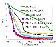
(a) Loss vs iterations: $n=10$

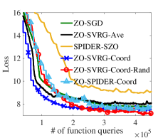
(b) Loss vs queries: $n=10$

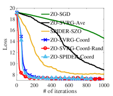
(c) Loss vs iterations: $n=100$

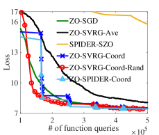
(d) Loss vs queries: $n=100$

Figure 1: Comparison of different zeroth-order algorithms for generating black-box adversarial examples for digit “1” class

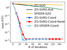
(a) Loss vs iterations: german

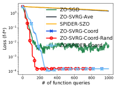
(b) Loss vs queries: german

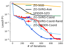
(c) Loss vs iterations: ijcnn1

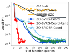
(d) Loss vs queries: ijcnn1

Figure 2: Comparison of different zeroth-order algorithms for logistic regression problem with a nonconvex regularizer

4.1 Generation of Black-Box Adversarial Examples

In image classification, adversary attack crafts input images with imperceptive perturbation to mislead a trained classifier. The resulting perturbed images are called adversarial examples, which are commonly used to understand the robustness of learning models. In the black-box setting, the attacker can access only the model evaluations, and hence the problem falls into the framework of zeroth-order optimization.

We use a well-trained DNN $F(\cdot)=[F_{1}(\cdot),...,F_{K}(\cdot)]$ for the MNIST handwritten digit classification as the target black-box model, where $F_{k}(\cdot)$ returns the prediction score of the $k^{th}$ class. We attack a batch of $n$ correctly-classified images $\{\mathbf{a}_{i}\}_{i=1}^{n}$ from the same class, and adopt the same black-box attacking loss as in Chen et al. 2017; Liu et al. 2018b. The $i^{th}$ individual loss function $f_{i}(\mathbf{x})$ is given by

$$f_{i}(\mathbf{x})= \max\big{\{}\log F_{y_{i}}\left(\mathbf{a}^{adv}_{i}\right)-\max_{t\neq y_{i}}\log F_{t}\left(\mathbf{a}_{i}^{adv}\right),0\big{\}}$$

$$+\lambda\|\mathbf{a}^{adv}_{i}-\mathbf{a}_{i}\|^{2},$$

where $\mathbf{a}^{adv}_{i}=0.5\tanh\left(\tanh^{-1}\left(2\mathbf{a}_{i}\right)+\mathbf{x}\right)$ is the adversarial example of the $i^{th}$ natural image $\mathbf{a}_{i}$, and $y_{i}$ is the true label of image $\mathbf{a}_{i}$. In our experiment, we set the regularization parameter $\lambda=1$ for digit “1” image class, and set $\lambda=0.1$ for digit “4” class.

Fig. 1 and Fig. 3 (in the supplementary materials) provide comparison of the performance for the algorithms of interest. Two major observations can be made. First, our proposed two algorithms ZO-SVRG-Coord-Rand and ZO-SPIDER-Coord as well as ZO-SVRG-Coord (with the large stepsize due to our improved analysis) have much better performance both in convergence rate (iteration complexity) and function query complexity than ZO-SGD, ZO-SVRG-Ave and SPIDER-SZO. Among them, ZO-SVRG-Coord-Rand achieves the best performance. Second, our ZO-SPIDER-Coord algorithm converges much faster than SPIDER-SZO in the initial optimization stage, and more importantly, has much lower function query complexity, which is largely due to the $\epsilon$-level stepsize required by SPIDER-SZO. In addition, we present the generated adversarial examples for attacking digit “4” class in Table 3 in the supplementary materials, where our ZO-SVRG-Coord-Rand achieves the lowest image distortion.

Interestingly, though SPIDER-based algorithms have been shown to outperfom SVRG-based algorithms in theory, our experiments suggest that SVRG-based algorithms in fact achieve comparable and sometimes even better performance in practice. The same observations have also been made in Fang et al. 2018 and Nguyen et al. 2017a, b.

4.2 Nonconvex Logistic Regression

In this subsection, we consider the following zeroth-order nonconvex logistic regression problem with two classes $\min_{\mathbf{w}\in\mathbb{R}^{d}}\frac{1}{n}\sum_{i=1}^{n}\ell(\mathbf{w}^{T}\mathbf{x}_{i},y_{i})+\alpha\sum_{i=1}^{d}\frac{w_{i}^{2}}{1+w_{i}^{2}}$, where $\mathbf{x}_{i}\in\mathbb{R}^{d}$ denote the features, $y_{i}\in\{\pm 1\}$ are the classification labels, $\ell$ is the cross-entropy loss, and we set $\alpha=0.1$. For this problem, we use two datasets from LIBSVM (Chang & Lin, 2011): the german dataset ($n=1000,d=24$) and the ijcnn1 dataset ($n=49990,d=22$).

As shown in Fig. 2, ZO-SVRG-Coord-Rand, ZO-SVRG-Coord and ZO-SPIDER-Coord converges much faster than ZO-SGD , ZO-SVRG-Ave and SPIDER-SZO in terms of number of iterations for both datasets. In terms of function query complexity, ZO-SVRG-Coord converges much faster than ZO-SVRG-Ave for both datasets and slightly faster than ZO-SGD for ijcnn1 dataset, which corroborates our new complexity analysis for ZO-SVRG-Coord. The convergence and complexity performance of ZO-SPIDER-Coord is similar to ZO-SVRG-Coord. Among these algorithms, ZO-SVRG-Coord-Rand has the best function query complexity for both datasets.

5 Conclusion

In this paper, we developed two novel zeroth-order variance-reduced algorithms named ZO-SVRG-Coord-Rand and ZO-SPIDER-Coord as well as an improved analysis on ZO-SVRG-Coord proposed by Liu et al. 2018b. We showed that ZO-SVRG-Coord-Rand and ZO-SVRG-Coord (under our new analysis) outperform ZO-GD, ZO-SGD and all other existing SVRG-based zeroth-order algorithms. Furthermore, compared with SPIDER-SZO (Fang et al., 2018), our ZO-SPIDER-Coord allows a much larger constant stepsize and is free from the generation of a large number of Gaussian random variables while maintaining the same function query complexity. Our experiments demonstrate the superior performance of our proposed algorithms.

Supplementary Materials

Appendix A Further Specification of Experiments and Additional Results

A.1 Generation of Black-Box Adversarial Examples

Parameter selection for algorithms under comparison. For ZO-SGD and ZO-SVRG-Ave, we adopt the implementations from Liu et al. 2018b. As recommended by Liu et al. 2018b, we set the epoch length $q=10$ for ZO-SVRG-Ave, and select the mini-batch size $|\mathcal{S}_{2}|$ from $\{5,10,50\}$ and the stepsize $\eta$ from $\{1,10,20,30,40\}/d$ for both ZO-SGD and ZO-SVRG-Ave, and we present the best performance among these parameters, where $d=28\times 28$ is the input dimension. For SPIDER-SZO, we set the parameters by Theorem 8 in Fang et al. 2018. Namely, we choose the epoch length $q$ from $\{30,50,80\}$, mini-batch size $|\mathcal{S}_{2}|$ from $\{5,80,700\}$, and $\eta$ from $\{0.1,0.01\}/\|\mathbf{v}^{k}\|$, and we present the best performance among these parameters. The parameters chosen for our ZO-SVRG-Coord-Rand, ZO-SVRG-Coord (based on our new analysis, which allows a larger stepsize with performance guarantee) and ZO-SPIDER-Coord are listed in Table 4. For all algorithms, we choose $|\mathcal{S}_{1}|=n$, and set the smoothing parameters $\beta=0.01$ and $\delta=0.001$.

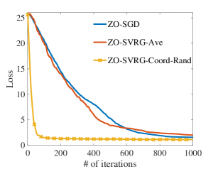
(a) Loss vs iterations: $n=10$

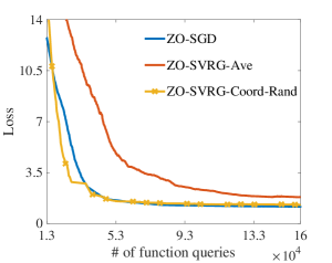
(b) Loss vs queries: $n=10$

Figure 3: Comparison of different zeroth-order algorithms for generating black-box adversarial examples for digit “4” class

Table 3: Generated adversarial examples for digit “4” class, where image distortion is defined as $\frac{1}{n}\sum_{i=1}^{n}\|\mathbf{a}^{adv}_{i}-\mathbf{a}_{i}\|^{2}$.

Image ID $4$ $6$ $19$ $24$ $27$ $33$ $42$ $48$ $49$ $56$ Image distortion ZO-SGD $11.46$ Classified as $\bf 9$ $\bf 8$ $\bf 1$ $\bf 3$ $\bf 2$ $\bf 2$ $\bf 9$ $\bf 9$ $\bf 9$ $\bf 9$ ZO-SVRG-Ave $13.85$ Classified as $\bf 9$ $\bf 8$ $\bf 2$ $\bf 3$ $\bf 2$ $\bf 2$ $\bf 9$ $\bf 9$ $\bf 9$ $\bf 3$ ZO-SVRG-Coord-Rand $11.21$ Classified as $\bf 9$ $\bf 8$ $\bf 2$ $\bf 3$ $\bf 2$ $\bf 2$ $\bf 9$ $\bf 9$ $\bf 9$ $\bf 9$

Table 4: Parameter settings for ZO-SVRG-Coord-Rand (left), ZO-SVRG-Coord (middle) and ZO-SPIDER-Coord (right).

Parameters	$n=10$	$n=100$
$q$	$50$	$80$
$|\mathcal{S}_{2}|$	$80$	$700$
$\eta$	$0.102$	$0.663$

Parameters	$n=10$	$n=100$
$q$	$30$	$50$
$|\mathcal{S}_{2}|$	$5$	$70$
$\eta$	$0.102$	$0.255$

Parameters	$n=10$	$n=100$
$q$	$30$	$50$
$|\mathcal{S}_{2}|$	$5$	$70$
$\eta$	$0.064$	$0.255$

A.2 Nonconvex logistic regression

Parameter selection for algorithms under comparison. For all algorithms, we choose fixed mini-batch sizes $|\mathcal{S}_{1}|=n$ and $|\mathcal{S}_{2}|=128$, the epoch length $q=n/128$ for german dataset, and choose fixed mini-batch sizes $|\mathcal{S}_{1}|=50*256$ and $|\mathcal{S}_{2}|=256$, the epoch length $q=n/256$ for ijcnn1 dataset. In addition, we set the learning rate for all algorithms according to their convergence guarantee. In specific, we choose $\eta=0.8$ for ZO-SVRG-Coord-Rand, ZO-SPIDER-Coord, ZO-SVRG-Coord, and choose $\eta=0.8/d$ for ZO-SGD, ZO-SVRG-Ave, and set $\eta=0.8\sqrt{\epsilon}/\|v_{k}\|$ for SPIDER-SZO, as specified in Fang et al. 2018.

Appendix B Zeroth-Order Nonconvex Nonsmooth Composite Optimization

Zeroth-order optimization has been studied for nonconvex and nonsmooth objective function in (Ghadimi et al., 2016), where a zeroth-order stochastic algorithm named RSPGF has been proposed. Here, we propose a zeroth-order stochastic variance-reduced algorithm for the same objective function, and show that it order-wisely outperforms RSPGF.

B.1 PROX-ZO-SPIDER-Coord for Composite Optimization

In this subsection, we extend our study of ZO-SPIDER-Coord to the following nonconvex and nonsmooth composite problem

$$\min_{\mathbf{x}\in\mathbb{R}^{d}}\Psi(\mathbf{x})=f(\mathbf{x})+h(\mathbf{x}),f(x)=\frac{1}{n}\sum_{i=1}^{n}f_{i}(\mathbf{x}),$$ (15)

where each $f_{i}(\mathbf{x})$ is smooth and nonconvex, $h(\mathbf{x})$ is a nonsmooth convex function ( e.g., $h(\mathbf{x})=\lambda\|\mathbf{x}\|_{1},\lambda>0$). To address the nonsmooth term $h(\mathbf{x})$ in the objective function (15), we propose PROX-ZO-SPIDER-Coord algorithm, which replaces line 8 in Algorithm 2 by a proximal gradient step

$$\quad\mathbf{x}^{k+1}=\arg\min_{\mathbf{x}\in\mathbb{R}^{d}}\big{\{}\langle\mathbf{v}^{k},\mathbf{x}\rangle+\frac{1}{2\eta}\|\mathbf{x}-\mathbf{x}^{k}\|^{2}+h(\mathbf{x})\big{\}}.$$

Similarly to Ghadimi et al. 2016, we define

$$G(\mathbf{x},\nabla f(\mathbf{x}),\eta)=\frac{1}{\eta}\left(\mathbf{x}-\mathbf{x}^{+}\right)$$ (16)

as a generalized projected gradient of $\Psi(\cdot)$ at the point $\mathbf{x}$ and use it to characterize the convergence criterion, where the point $\mathbf{x}^{+}$ is given by the proximal mapping

$$\mathbf{x}^{+}=\arg\min_{\mathbf{z}\in\mathbb{R}^{d}}\left\{\langle\nabla f(\mathbf{x}),\mathbf{z}\rangle+\frac{1}{2\eta}\|\mathbf{z}-\mathbf{x}\|^{2}+h(\mathbf{z})\right\}.$$

Based on the above notations, we provide the following convergence guarantee for PROX-ZO-SPIDER-Coord.

Theorem 5.

Let Assumption 1 hold, and we choose the same parameters as in Corollary 3. Then our PROX-ZO-SPIDER-Coord satisfies $\mathbb{E}\|G(\mathbf{x}^{\zeta},\nabla f(\mathbf{x}^{\zeta}),\eta)\|^{2}\leq(60\Delta_{\psi}L+80+69\sigma^{2})/K+138/K^{2}$, where $0<\Delta_{\psi}=\psi(\mathbf{x}^{0})-\psi(\mathbf{x}^{*})<\infty$ and $\mathbf{x}^{*}=\arg\min_{\mathbf{x}\in\mathbb{R}^{d}}\psi(\mathbf{x})$.

To achieve $\mathbb{E}\|G(\mathbf{x}^{\zeta},\nabla f(\mathbf{x}^{\zeta}),\eta)\|^{2}\leq\epsilon$, the number of function queries is at most $\mathcal{O}\left(\min\left\{n^{1/2}d\epsilon^{-1},d\epsilon^{-3/2}\right\}\right)$.

Let us compare our PROX-ZO-SPIDER-Coord algorithm with the randomized stochastic projected gradient free algorithm RSPGF, introduced by Ghadimi et al. 2016. Casting Corollary 8 in Ghadimi et al. 2016 to the setting of our Theorem 5 yields $\mathbb{E}\|G(\mathbf{x}^{\zeta},\nabla f(\mathbf{x}^{\zeta}),\eta)\|^{2}\leq\mathcal{O}\left(\frac{d}{\widetilde{K}}+\frac{\sqrt{d}}{\sqrt{\widetilde{K}}}\right)$, where $\widetilde{K}$ is the total number of function queries. Thus, RSPGF requires at most $\mathcal{O}(d/\epsilon^{2})$ function queries to achieve $\mathbb{E}\|G(\mathbf{x}^{\zeta},\nabla f(\mathbf{x}^{\zeta}),\eta)\|^{2}\leq\epsilon<1$. As a comparison, the function query complexity of PROX-ZO-SPIDER-Coord outperforms that of RSPGF (Ghadimi et al., 2016) by a factor of $\mathcal{O}(\max\{\epsilon^{-1}n^{-1/2},\epsilon^{-1/2}\})$.

Appendix C Zeroth-Order Variance-Reduced Algorithms for Convex Optimization

In this paper, we have proposed two new zeroth-order variance-reduced algorithms ZO-SVRG-Coord-Rand and ZO-SPIDER-Coord, and have studied their performance for nonconvex optimization. In this section, we study the performance of these two algorithms for convex optimization, where each individual function $f_{i}(\cdot)$ is convex. We note that there was no proven convergence guarantee for previously proposed zeroth-order SVRG-based and SPIDER-based algorithms for convex optimization.

C.1 ZO-SVRG-Coord-Rand-C Algorithm

In this subsection, we explore the convergence performance of ZO-SVRG-Coord-Rand for convex optimization. To fully utilize the convexity of the objective function, we propose a variant of our ZO-SVRG-Coord-Rand, which we refer to as ZO-SVRG-Coord-Rand-C. Differently from ZO-SVRG-Coord-Rand, the outer-loop iteration (i.e., $k\mod q=0$) of ZO-SVRG-Coord-Rand-C chooses $\mathbf{x}^{k}$ from $\{\mathbf{x}^{k-q},...,\mathbf{x}^{k-1}\}$ uniformly at random, which is a typical treatment used in convex first-order optimization (Reddi et al., 2016a; Nguyen et al., 2017a). In the meanwhile, the inner-loop iteration of ZO-SVRG-Coord-Rand-C is the same as single-sample ZO-SVRG-Coord-Rand, which computes $\mathbf{v}^{k}=\hat{\nabla}_{\text{rand}}f_{i_{k}}(\mathbf{x}^{k};\mathbf{u}^{k})-\hat{\nabla}_{\text{rand}}f_{i_{k}}(\mathbf{x}^{qk_{0}};\mathbf{u}^{k})+\mathbf{v}^{qk_{0}}$ with a single sample $i_{k}$ drawn from $[n]$ and a smoothing vector $\mathbf{u}^{k}$ drawn from the uniform distribution over the unit sphere. .

The following theorem provides the function query complexity for ZO-SVRG-Coord-Rand-C.

Theorem 6.

Under Assumption 1, let $\eta=1/(27dL),\beta=\epsilon/(c_{\beta}dL),\delta=\epsilon/(c_{\delta}\sqrt{d}L),q=c_{q}d/\epsilon$, $h=\log_{2}(c_{h}/\epsilon))$ and $|\mathcal{S}|=\min\{n,\lceil c_{s}/\epsilon\rceil\}$, where $c_{q},c_{h},c_{\beta},c_{\delta}$ and $c_{s}$ are sufficiently large positive constants. Then, to achieve an $\epsilon$-accuracy solution, i.e., $\mathbb{E}(f(\mathbf{x}^{K})-f(\mathbf{x}^{*}))\leq\epsilon$, the number of function queries required by ZO-SVRG-Coord-Rand-C algorithm is at most $\mathcal{O}(d\min\{n,1/\epsilon\}\log(1/\epsilon))$.

Let us compare our result with that of ZO-SGD given by Ghadimi & Lan 2013. Casting Corollary 3.3 in Ghadimi & Lan 2013 under the setting of our Corollary 6 implies that the function query complexity of ZO-SGD is $\mathcal{O}(d/\epsilon^{2})$, which is worse than that of our ZO-SVRG-Coord-Rand-C by a factor of $\mathcal{\widetilde{O}}(\max\{\epsilon^{-2}n^{-1},\epsilon^{-1}\})$.

C.2 ZO-SPIDER-Coord-C Algorithm

In this subsection, we generalize our ZO-SPIDER-Coord to solving convex optimization problem, and proposes the ZO-SPIDER-Coord-C algorithm. ZO-SPIDER-Coord-C has the same outer-loop iteration as ZO-SVRG-Coord-Rand-C, but updates $\mathbf{v}^{k}$ in a different way by $\mathbf{v}^{k}=\hat{\nabla}_{\text{coord}}f_{i_{k}}(\mathbf{x}^{k})-\hat{\nabla}_{\text{coord}}f_{i_{k}}(\mathbf{x}^{k-1})+\mathbf{v}^{k-1}$ at each inner-loop iteration.

Based on Lemma 6, we obtain the following complexity result for ZO-SPIDER-Coord-C.

Theorem 7.

Under Assumption 1, let $\eta=1/(24L),q=c_{q}/\epsilon$, $h=\log_{2}(c_{h}/\epsilon)),\delta=\epsilon/(c_{q}\sqrt{d}L)$ and $|\mathcal{S}|=\min\{n,\lceil c_{s}/\epsilon\rceil\}$, where $c_{q},c_{h}$ and $c_{s}$ are sufficiently large positive constants. Then, to achieve an $\epsilon$-accuracy solution, i.e., $\mathbb{E}\|\nabla f(\mathbf{x}^{K})\|^{2}\leq\epsilon$, the number of function queries required by ZO-SPIDER-Coord-C is at most $\mathcal{O}(d\min\{n,1/\epsilon\}\log(1/\epsilon))$

Note that ZO-SPIDER-Coord-C achieves the same function query complexity as that of ZO-SVRG-Coord-Rand-C, and improves that of ZO-SGD (Ghadimi & Lan, 2013) by a factor of $\mathcal{\widetilde{O}}(\max\{\epsilon^{-2}n^{-1},\epsilon^{-1}\})$ w.r.t. stationary gap $\mathbb{E}\|\nabla f(\mathbf{x}^{K})\|^{2}$. The detailed comparison among our algorithms and other exiting algorithms is summarized in Table 5.

Table 5: Comparison of zeroth-order algorithms in terms of the function query complexity for convex optimization.

Algorithms		Function query complexity	Function value convergence
ZO-SGD	(Ghadimi & Lan, 2013)	$\mathcal{O}\left(\frac{d}{\epsilon^{2}}\right)$	✓
ZSCG	(Balasubramanian & Ghadimi, 2018)	$\mathcal{O}\left(\frac{d}{\epsilon^{3}}\right)$	✓
M-ZSCG	(Balasubramanian & Ghadimi, 2018)	$\mathcal{O}\left(\frac{d}{\epsilon^{2}}\right)$	✓
ZO-SPIDER-Coord-C	(This work)	$\mathcal{O}(\min\{dn,\frac{d}{\epsilon}\}\log\left(\frac{1}{\epsilon}\right))$	✗
ZO-SVRG-Coord-Rand-C	(This work)	$\mathcal{O}(\min\{dn,\frac{d}{\epsilon}\}\log\left(\frac{1}{\epsilon}\right))$	✓

Technical Proofs

Appendix D Proof for ZO-SVRG-Coord-Rand

D.1 Auxiliary Lemmas

Before proving our main results, we first establish three useful lemmas.

Lemma 3.

For any given smoothing parameter $\delta>0$ and any $\mathbf{x}\in\mathbb{R}^{d}$, we have

$$\|\hat{\nabla}_{\text{coord}}f(\mathbf{x})-\nabla f(\mathbf{x})\|^{2}\leq L^{2}d\delta^{2}.$$

Proof.

Applying the mean value theorem (MVT) to the gradient $\nabla f(\mathbf{x})$, we have, for any given $\delta>0$,

$$\|\hat{\nabla}_{\text{coord}}f(\mathbf{x})-\nabla f(\mathbf{x})\|^{2} =\Big{\|}\frac{1}{2\delta}\sum_{i=1}^{d}(2\delta\mathbf{e}_{i}\mathbf{e}_{i}^{T}\nabla f(\mathbf{x}+(2t_{i}-1)\delta\mathbf{e}_{i}))-\nabla f(\mathbf{x})\Big{\|}^{2},\;\text{for }\,0<t_{i}<1,$$

$$\overset{\text{(i)}}{=}\sum_{i=1}^{d}\Big{\|}\mathbf{e}_{i}\mathbf{e}_{i}^{T}(\nabla f(\mathbf{x}+(2t_{i}-1)\delta\mathbf{e}_{i})-\nabla f(\mathbf{x}))\Big{\|}^{2}$$

$$\leq\sum_{i=1}^{d}\Big{\|}\nabla f(\mathbf{x}+(2t_{i}-1)\delta\mathbf{e}_{i})-\nabla f(\mathbf{x})\Big{\|}^{2}\overset{\text{(ii)}}{\leq}L^{2}\sum_{i=1}^{d}\|(2t_{i}-1)\delta\mathbf{e}^{i}\|^{2}\leq L^{2}d\delta^{2}$$

where (i) follows from the definition of $\mathbf{e}_{i}$ and Euclidean norm, and (ii) follows from Assumption 1. ∎

Lemma 4.

For any given $k_{0}\leq\lfloor K/q\rfloor$, we have

$$\mathbb{E}\|\mathbf{v}^{qk_{0}}-\hat{\nabla}_{\text{coord}}f(\mathbf{x}^{qk_{0}})\|^{2}\leq\frac{3I(|\mathcal{S}_{1}|<n)}{|\mathcal{S}_{1}|}\left(2L^{2}d\delta^{2}+\sigma^{2}\right),$$

where $I(\cdot)$ is the indicator function.

Proof.

To simplify notation, we let $\mathbf{z}_{j}=\hat{\nabla}_{\text{coord}}f_{j}(\mathbf{x}^{qk_{0}})-\hat{\nabla}_{\text{coord}}f(\mathbf{x}^{qk_{0}})$ and $I_{j}=I(j\in\mathcal{S}_{1})$, where $I(\cdot)$ is the indicator function. First note that $\mathbb{E}(I^{2}_{j})=\frac{|\mathcal{S}_{1}|}{n}\;\;\text{and}\;\;\mathbb{E}I_{i}I_{j}=C^{2}_{|\mathcal{S}_{1}|}/C_{n}^{2}=\frac{|\mathcal{S}_{1}|(|\mathcal{S}_{1}|-1)}{n(n-1)},i\neq j$. Then, based on the above equalities, we have

$$\mathbb{E}\|\mathbf{v}^{qk_{0}}-\hat{\nabla}_{\text{coord}}f(\mathbf{x}^{qk_{0}})\|^{2}=\frac{1}{|\mathcal{S}_{1}|^{2}}\left(\sum_{j=1}^{n}\mathbb{E}I_{j}^{2}\Big{\|}\mathbf{z}_{j}\Big{\|}^{2}+\sum_{i\neq j}\mathbb{E}I_{i}I_{j}\big{\langle}\mathbf{z}_{i},\mathbf{z}_{j}\big{\rangle}\right)$$

$$=\frac{1}{|\mathcal{S}_{1}|^{2}}\left(\frac{|\mathcal{S}_{1}|}{n}\sum_{j=1}^{n}\Big{\|}\mathbf{z}_{j}\Big{\|}^{2}+\frac{|\mathcal{S}_{1}|(|\mathcal{S}_{1}|-1)}{n(n-1)}\sum_{i\neq j}\big{\langle}\mathbf{z}_{i},\mathbf{z}_{j}\big{\rangle}\right)$$

$$=\frac{1}{|\mathcal{S}_{1}|^{2}}\left(\left(\frac{|\mathcal{S}_{1}|}{n}-\frac{|\mathcal{S}_{1}|(|\mathcal{S}_{1}|-1)}{n(n-1)}\right)\sum_{j=1}^{n}\Big{\|}\mathbf{z}_{j}\Big{\|}^{2}+\frac{|\mathcal{S}_{1}|(|\mathcal{S}_{1}|-1)}{n(n-1)}\left\|\sum_{j=1}^{n}\mathbf{z}_{j}\right\|^{2}\right)$$

$$=\frac{n-|\mathcal{S}_{1}|}{(n-1)|\mathcal{S}_{1}|}\frac{1}{n}\sum_{j=1}^{n}\Big{\|}\mathbf{z}_{j}\Big{\|}^{2}+\frac{(|\mathcal{S}_{1}|-1)}{n(n-1)|\mathcal{S}_{1}|}\left\|\sum_{j=1}^{n}\mathbf{z}_{j}\right\|^{2}$$

$$\leq\frac{I(|\mathcal{S}_{1}|<n)}{|\mathcal{S}_{1}|}\frac{1}{n}\sum_{j=1}^{n}\Big{\|}\mathbf{z}_{j}\Big{\|}^{2}+\frac{1}{n^{2}}\left\|\sum_{j=1}^{n}\mathbf{z}_{j}\right\|^{2}$$

$$=\frac{I(|\mathcal{S}_{1}|<n)}{|\mathcal{S}_{1}|}\frac{1}{n}\sum_{j=1}^{n}\Big{\|}\hat{\nabla}_{\text{coord}}f_{j}(\mathbf{x}^{qk_{0}})-\hat{\nabla}_{\text{coord}}f(\mathbf{x}^{qk_{0}})\Big{\|}^{2}$$

$$\leq\frac{3I(|\mathcal{S}_{1}|<n)}{|\mathcal{S}_{1}|}\frac{1}{n}\sum_{j=1}^{n}\Big{(}\|\hat{\nabla}_{\text{coord}}f_{j}(\mathbf{x}^{qk_{0}})-\nabla f_{j}(\mathbf{x}^{qk_{0}})\|^{2}+\|\nabla f_{j}(\mathbf{x}^{qk_{0}})-\nabla f(\mathbf{x}^{qk_{0}})\|^{2}$$

$$\quad+\|\hat{\nabla}_{\text{coord}}f(\mathbf{x}^{qk_{0}})-\nabla f(\mathbf{x}^{qk_{0}})\|^{2}\Big{)}\leq\frac{3I(|\mathcal{S}_{1}|<n)}{|\mathcal{S}_{1}|}\left(2L^{2}d\delta^{2}+\sigma^{2}\right),$$

where the last inequality follows from Assumption 1 and Lemma 3. Then, the proof is complete. ∎

Lemma 5.

Let $f_{\beta}(\mathbf{x})=\mathbb{E}_{\mathbf{u}\sim\text{U}_{B}}\left(f(\mathbf{x}+\beta\mathbf{u})\right)$ be a smooth approximation of $f(\mathbf{x})$, where $\text{U}_{B}$ is the uniform distribution over the $d$-dimensional unit Euclidean ball $B$. Then,

1. $|f_{\beta}(\mathbf{x})-f(\mathbf{x})|\leq\frac{\beta^{2}L}{2}$ and $\|\nabla f_{\beta}(\mathbf{x})-\nabla f(\mathbf{x})\|\leq\frac{\beta Ld}{2}\,$ for any $\mathbf{x}\in\mathbb{R}^{d}$

2. $\mathbb{E}_{k}\left(\frac{1}{|\mathcal{S}_{2}|}\sum_{j=1}^{|\mathcal{S}_{2}|}\hat{\nabla}_{\text{rand}}f_{a_{j}}(\mathbf{x};\mathbf{u}_{j}^{k})\right)=\nabla f_{\beta}(\mathbf{x})$, where $\mathbf{x}$ is either $\mathbf{x}^{k}\text{ or }\mathbf{x}^{qk_{0}}$

3. $\mathbb{E}_{k}\left\|\hat{\nabla}_{\text{rand}}f_{a_{j}}(\mathbf{x}^{k};\mathbf{u}_{j}^{k})-\hat{\nabla}_{\text{rand}}f_{a_{j}}(\mathbf{x}^{qk_{0}};\mathbf{u}_{j}^{k})\right\|^{2}\\ \leq 3d^{2}\mathbb{E}_{k}\langle\nabla f_{a_{j}}(\mathbf{x}^{k})-\nabla f_{a_{j}}(\mathbf{x}^{qk_{0}}),\mathbf{u}_{j}^{k}\rangle^{2}+\frac{3L^{2}d^{2}\beta^{2}}{2}\\ \leq 3dL^{2}\|\mathbf{x}^{k}-\mathbf{x}^{qk_{0}}\|^{2}+\frac{3L^{2}d^{2}\beta^{2}}{2}$,

where the shorthand $\mathbb{E}_{k}(\cdot)=\mathbb{E}(\cdot\;|\mathbf{x}^{0},....,\mathbf{x}^{k}\;)$.

Proof.

The proof of item (1) directly follows from Lemma 4.1 in Gao et al. 2014.

We next prove item (2). Based on the equation (3.4) in Gao et al. 2014, we have

$$\nabla f_{\beta}(\mathbf{x}^{k})= \mathbb{E}_{\mathbf{u}\sim{\text{ U}}_{S_{p}}}\Big{(}\frac{d}{\beta}f(\mathbf{x}^{k}+\beta\mathbf{u})\mathbf{u}\Big{)}\overset{\text{(i)}}{=}\mathbb{E}_{\mathbf{u}\sim{\text{ U}}_{S_{p}}}\left(\frac{d}{\beta}\Big{(}f(\mathbf{x}^{k}+\beta\mathbf{u})-f(\mathbf{x}^{k})\Big{)}\mathbf{u}\right)$$

$$= \mathbb{E}_{\mathbf{u}\sim{\text{ U}}_{S_{p}}}\Big{(}\frac{1}{n}\sum_{i=1}^{n}\frac{d}{\beta}\left(f_{i}(\mathbf{x}^{k}+\beta\mathbf{u})-f_{i}(\mathbf{x}^{k})\right)\mathbf{u}\Big{)}=\frac{1}{n}\sum_{i=1}^{n}\mathbb{E}_{\mathbf{u}\sim{\text{ U}}_{S_{p}}}\Big{(}\frac{d}{\beta}\left(f_{i}(\mathbf{x}^{k}+\beta\mathbf{u})-f_{i}(\mathbf{x}^{k})\right)\mathbf{u}\Big{)},$$ (17)

where the random vector $\mathbf{u}$ is independent of $\mathbf{x}^{k}$, $\text{U}_{S_{p}}$ is the uniform distribution over the unit sphere $S_{p}$ and (i) follows from the fact that $\mathbb{E}_{\mathbf{u}\sim{\text{ U}}_{S_{p}}}\left(f(\mathbf{x}^{k})\mathbf{u}\right)=0$. To simplify notation, we let $\mathbb{E}_{k}(\cdot)=\mathbb{E}(\cdot|\mathbf{x}^{1},...,\mathbf{x}^{k})$. Conditioned on $\mathbf{x}^{0},....,\mathbf{x}^{k}$ and noting that the random samples in $\mathcal{S}_{2}$ and $\mathbf{u}_{j}^{k},j=1,...,|\mathcal{S}_{2}|$ generated at the $k^{th}$ iteration are independent of $\mathbf{x}^{0},....,\mathbf{x}^{k}$, we have

$$\mathbb{E}_{k} \bigg{(}\frac{d}{\beta|\mathcal{S}_{2}|}\sum_{j=1}^{|\mathcal{S}_{2}|}(f_{a_{j}}(\mathbf{x}^{k}+\beta\mathbf{u}_{j}^{k})-f_{a_{j}}(\mathbf{x}^{k}))\mathbf{u}_{j}^{k}\bigg{)}=\frac{1}{|\mathcal{S}_{2}|}\sum_{j=1}^{|\mathcal{S}_{2}|}\mathbb{E}_{k}\bigg{(}\frac{d}{\beta}(f_{a_{j}}(\mathbf{x}^{k}+\beta\mathbf{u}_{j}^{k})-f_{a_{j}}(\mathbf{x}^{k}))\mathbf{u}_{j}^{k}\bigg{)}$$

$$=\frac{1}{|\mathcal{S}_{2}|}\sum_{j=1}^{|\mathcal{S}_{2}|}\mathbb{E}_{k}\bigg{(}\mathbb{E}_{a_{j}}\Big{(}\frac{d}{\beta}(f_{a_{j}}(\mathbf{x}^{k}+\beta\mathbf{u}_{j}^{k})-f_{a_{j}}(\mathbf{x}^{k}))\mathbf{u}_{j}^{k}\,\Big{|}\,\mathbf{u}_{j}^{k}\Big{)}\bigg{)}$$

$$\overset{\text{(i)}}{=}\frac{1}{|\mathcal{S}_{2}|}\sum_{j=1}^{|\mathcal{S}_{2}|}\mathbb{E}_{k}\bigg{(}\frac{1}{n}\sum_{i=1}^{n}\frac{d}{\beta}(f_{i}(\mathbf{x}^{k}+\beta\mathbf{u}_{j}^{k})-f_{i}(\mathbf{x}^{k}))\mathbf{u}_{j}^{k}\bigg{)}$$

$$\overset{\text{(ii)}}{=}\frac{1}{|\mathcal{S}_{2}|}\sum_{j=1}^{|\mathcal{S}_{2}|}\left(\nabla f_{\beta}(\mathbf{x}^{k})\right)=\nabla f_{\beta}(\mathbf{x}^{k}),$$ (18)

where (i) follows from the definition of the set $\mathcal{S}_{1}$ and (ii) follows from (D.1). Taking steps similar to (D.1) and conditioning on $\mathbf{x}^{0},...,\mathbf{x}^{k}$, we have

$$\mathbb{E}_{k} \bigg{(}\frac{d}{\beta|\mathcal{S}_{2}|}\sum_{j=1}^{|\mathcal{S}_{2}|}(f_{a_{j}}(\mathbf{x}^{qk_{0}}+\beta\mathbf{u}_{j}^{k})-f_{a_{j}}(\mathbf{x}^{k}))\mathbf{u}_{j}^{k}\bigg{)}=\nabla f_{\beta}(\mathbf{x}^{qk_{0}}).$$ (19)

Our final step is to prove item (3). Note that

$$\mathbb{E}\bigg{\|} \frac{d(f_{a_{j}}(\mathbf{x}^{k}+\beta\mathbf{u}_{j}^{k})-f_{a_{j}}(\mathbf{x}^{k}))}{\beta}\mathbf{u}_{j}^{k}-\frac{d(f_{a_{j}}(\mathbf{x}^{qk_{0}}+\beta\mathbf{u}_{j}^{k})-f_{a_{j}}(\mathbf{x}^{qk_{0}}))}{\beta}\mathbf{u}_{j}^{k}\bigg{\|}^{2}$$

$$= d^{2}\mathbb{E}_{k}\bigg{\|}\frac{(f_{a_{j}}(\mathbf{x}^{k}+\beta\mathbf{u}_{j}^{k})-f_{a_{j}}(\mathbf{x}^{k})-\langle\nabla f_{a_{j}}(\mathbf{x}^{k}),\beta\mathbf{u}_{j}^{k}\rangle)\mathbf{u}_{j}^{k}}{\beta}+\left(\langle\nabla f_{a_{j}}(\mathbf{x}^{k}),\mathbf{u}_{j}^{k}\rangle\mathbf{u}_{j}^{k}-\langle\nabla f_{a_{j}}(\mathbf{x}^{qk_{0}}),\mathbf{u}_{j}^{k}\rangle\mathbf{u}_{j}^{k}\right)$$

$$-\frac{(f_{a_{j}}(\mathbf{x}^{qk_{0}}+\beta\mathbf{u}_{j}^{k})-f_{a_{j}}(\mathbf{x}^{qk_{0}})-\langle\nabla f_{a_{j}}(\mathbf{x}^{qk_{0}}),\beta\mathbf{u}_{j}^{k}\rangle)\mathbf{u}_{j}^{k}}{\beta}\bigg{\|}^{2}$$ (20)

Then, using the inequality that $f_{a_{j}}(\mathbf{y})-f_{a_{j}}(\mathbf{x})-\langle\nabla f_{a_{j}}(\mathbf{x}),\mathbf{y-x}\rangle\leq\frac{L}{2}\|\mathbf{y-x}\|^{2}$ in (D.1) yields

$$\mathbb{E}\bigg{\|} \frac{d(f_{a_{j}}(\mathbf{x}^{k}+\beta\mathbf{u}_{j}^{k})-f_{a_{j}}(\mathbf{x}^{k}))}{\beta}\mathbf{u}_{j}^{k}-\frac{d(f_{a_{j}}(\mathbf{x}^{qk_{0}}+\beta\mathbf{u}_{j}^{k})-f_{a_{j}}(\mathbf{x}^{qk_{0}}))}{\beta}\mathbf{u}_{j}^{k}\bigg{\|}^{2}$$

$$\leq 3d^{2}\mathbb{E}_{k}\|\langle\nabla f_{a_{j}}(\mathbf{x}^{k}),\mathbf{u}_{j}^{k}\rangle\mathbf{u}_{j}^{k}-\langle\nabla f_{a_{j}}(\mathbf{x}^{qk_{0}}),\mathbf{u}_{j}^{k}\rangle\mathbf{u}_{j}^{k}\|^{2}+\frac{3L^{2}d^{2}\beta^{2}}{2}$$

$$\overset{\text{(i)}}{=} 3d^{2}\mathbb{E}_{k}\langle\nabla f_{a_{j}}(\mathbf{x}^{k})-\nabla f_{a_{j}}(\mathbf{x}^{qk_{0}}),\mathbf{u}_{j}^{k}\rangle^{2}+\frac{3L^{2}d^{2}\beta^{2}}{2}$$

$$= 3d^{2}\left(\nabla f_{a_{j}}(\mathbf{x}^{k})-\nabla f_{a_{j}}(\mathbf{x}^{qk_{0}})\right)^{T}\mathbb{E}(\mathbf{u}_{j}^{k}(\mathbf{u}_{j}^{k})^{T})\left(\nabla f_{a_{j}}(\mathbf{x}^{k})-\nabla f_{a_{j}}(\mathbf{x}^{qk_{0}})\right)+\frac{3L^{2}d^{2}\beta^{2}}{2}$$ (21)

where (i) follows from the fact that $\|\mathbf{u}_{j}^{k}\|=1$. Based on the definition of $\mathbf{u}_{j}^{k}$ , we rewrite $\mathbf{u}_{j}^{k}=\mathbf{r}/\|\mathbf{r}\|$ and define a matrix $\mathbf{U}=\mathbb{E}(\mathbf{u}_{j}^{k}(\mathbf{u}_{j}^{k})^{T})$, where $\mathbf{r}$ is a $d$-dimensional Gaussian standard random vector. Let $\mathbf{r}(i)$ denote the $i^{th}$ entry of $\mathbf{r}$, and $\mathbf{U}(i,j)$ denote $(i,j)^{th}$ entry of $\mathbf{U}$. Then, we have, for $i=1,...,d$

$$\mathbf{U}(i,i)=\int\frac{\mathbf{r}(i)^{2}}{\sum_{t=1}^{d}\mathbf{r}(t)^{2}}e^{-\frac{\sum_{t=1}^{d}\mathbf{r}(t)^{2}}{2}}d\mathbf{r}(1)\cdots d.\mathbf{r}(d)$$ (22)

Since $\mathbf{r}(i),i=1,...,d$ are i.i.d. standard Gaussian random variables, we have

$$\mathbf{U}(1,1)=\cdots\mathbf{U}(d,d),\text{ and }\sum_{i=1}^{d}\mathbf{U}(i,i)=\int e^{-\frac{\sum_{t=1}^{d}\mathbf{r}(t)^{2}}{2}}d\mathbf{r}(1)\cdots d\mathbf{r}(d)=1,$$

which implies that $\mathbf{U}(i,i)=1/d$ for all $i=1,...,d$. In addition, for any $i\neq j$, we have

$$\mathbf{U}(i,j)=\int\frac{\mathbf{r}(i)\mathbf{r}(j)}{\sum_{t=1}^{d}\mathbf{r}(t)^{2}}e^{-\frac{\sum_{t=1}^{d}\mathbf{r}(t)^{2}}{2}}d\mathbf{r}(1)\cdots d\mathbf{r}(d),$$

which, noting the symmetry between $\mathbf{r}(i)$ and $\mathbf{r}(j)$, implies that $\mathbf{U}(i,j)=0$. Combining the above two results yields that $\mathbf{U}=\frac{1}{d}\mathbf{I}_{d}$, where $\mathbf{I}_{d}$ is a $d$-dimensional identity matrix. Thus, plugging $\mathbb{E}(\mathbf{u}_{j}^{k}(\mathbf{u}_{j}^{k})^{T})=\mathbf{U}=\frac{1}{d}\mathbf{I}_{d}$ in (D.1) yields

$$\mathbb{E}\bigg{\|} \frac{d(f_{a_{j}}(\mathbf{x}^{k}+\beta\mathbf{u}_{j}^{k})-f_{a_{j}}(\mathbf{x}^{k}))}{\beta}\mathbf{u}_{j}^{k}-\frac{d(f_{a_{j}}(\mathbf{x}^{qk_{0}}+\beta\mathbf{u}_{j}^{k})-f_{a_{j}}(\mathbf{x}^{qk_{0}}))}{\beta}\mathbf{u}_{j}^{k}\bigg{\|}^{2}$$

$$\leq 3d\|\nabla f_{a_{j}}(\mathbf{x}^{k})-\nabla f_{a_{j}}(\mathbf{x}^{qk_{0}})\|^{2}+\frac{3L^{2}d^{2}\beta^{2}}{2}\leq 3dL^{2}\|\mathbf{x}^{k}-\mathbf{x}^{qk_{0}}\|^{2}+\frac{3L^{2}d^{2}\beta^{2}}{2},$$ (23)

which finishes the proof. ∎

D.2 Proof of Lemma 1

Using Lemmas 3, 4, 5, we now prove Lemma 1. Based on the updating step of Algorithm 1, we obtain

$$\mathbf{v}^{k}-\nabla f_{\beta}(\mathbf{x}^{k})= \frac{d}{\beta|\mathcal{S}_{2}|}\sum_{j=1}^{|\mathcal{S}_{2}|}(f_{a_{j}}(\mathbf{x}^{k}+\beta\mathbf{u}_{j}^{k})-f_{a_{j}}(\mathbf{x}^{k}))\mathbf{u}_{j}^{k}-\nabla f_{\beta}(\mathbf{x}^{k})$$

$$-\frac{d}{\beta|\mathcal{S}_{2}|}\sum_{j=1}^{|\mathcal{S}_{2}|}(f_{a_{j}}(\mathbf{x}^{qk_{0}}+\beta\mathbf{u}_{j}^{k})-f_{a_{j}}(\mathbf{x}^{qk_{0}}))\mathbf{u}_{j}^{k}+\nabla f_{\beta}(\mathbf{x}^{qk_{0}})+\mathbf{v}^{qk_{0}}-\nabla f_{\beta}(\mathbf{x}^{qk_{0}}).$$ (24)

To simplify notation, we define

$$H_{j}(\mathbf{x})=\frac{d}{\beta}(f_{a_{j}}(\mathbf{x}+\beta\mathbf{u}_{j}^{k})-f_{a_{j}}(\mathbf{x}))\mathbf{u}_{j}^{k},\,\mathbf{x}=\mathbf{x}^{k}\text{ or }\,\mathbf{x}^{qk_{0}},$$

and use the shorthand $\mathbb{E}_{k}(\cdot)$ to denote $\mathbb{E}(\cdot\,|\,\mathbf{x}^{0},...,\mathbf{x}^{k})$. Then, using (D.2), we obtain

$$\mathbb{E}_{k}\|\mathbf{v}^{k}-\nabla f_{\beta}(\mathbf{x}^{k})\|^{2}\leq \frac{2}{|\mathcal{S}_{2}|}\mathbb{E}_{k}\|H_{j}(\mathbf{x}^{k})-H_{j}(\mathbf{x}^{qk_{0}})-(\nabla f_{\beta}(\mathbf{x}^{k})-\nabla f_{\beta}(\mathbf{x}^{qk_{0}}))\|^{2}$$

$$+2\sum_{i\neq j}\mathbb{E}_{k}\langle H_{i}(\mathbf{x}^{k})-H_{i}(\mathbf{x}^{qk_{0}})-(\nabla f_{\beta}(\mathbf{x}^{k})-\nabla f_{\beta}(\mathbf{x}^{qk_{0}})),H_{j}(\mathbf{x}^{k})-H_{j}(\mathbf{x}^{qk_{0}})$$

$$\quad-(\nabla f_{\beta}(\mathbf{x}^{k})-\nabla f_{\beta}(\mathbf{x}^{qk_{0}}))\rangle+2\|\mathbf{v}^{qk_{0}}-\nabla f_{\beta}(\mathbf{x}^{qk_{0}})\|^{2}$$

$$\overset{\text{(i)}}{=} \frac{2}{|\mathcal{S}_{2}|}\mathbb{E}_{k}\|H_{j}(\mathbf{x}^{k})-H_{j}(\mathbf{x}^{qk_{0}})-(\nabla f_{\beta}(\mathbf{x}^{k})-\nabla f_{\beta}(\mathbf{x}^{qk_{0}}))\|^{2}$$

$$+2\|\mathbf{v}^{qk_{0}}-\nabla f_{\beta}(\mathbf{x}^{qk_{0}})\|^{2}$$ (25)

where (i) follows from the fact that $a_{i}$ and $\mathbf{u}_{i}^{k}$ are independent of $a_{j}$ and $\mathbf{u}_{j}^{k}$ for any $i\neq j$, and from the following equalities

$$\mathbb{E}_{k}(H_{j}(\mathbf{x}^{k})) =\mathbb{E}_{\mathbf{u}_{j}^{k}}\Big{(}\frac{d}{\beta}f(\mathbf{x}^{k}+\beta\mathbf{u}_{j}^{k})\mathbf{u}_{j}^{k}\Big{)}=\nabla f_{\beta}(\mathbf{x}^{k})$$

$$\mathbb{E}_{k}(H_{j}(\mathbf{x}^{qk_{0}})) =\mathbb{E}_{\mathbf{u}_{j}^{k}}\Big{(}\frac{d}{\beta}f(\mathbf{x}^{qk_{0}}+\beta\mathbf{u}_{j}^{k})\mathbf{u}_{j}^{k}\Big{)}=\nabla f_{\beta}(\mathbf{x}^{qk_{0}}).$$ (26)

Then, we further simplify (D.2) to obtain

$$\mathbb{E}_{k}\|\mathbf{v}^{k}-\nabla f_{\beta}(\mathbf{x}^{k})\|^{2}\leq \frac{2}{|\mathcal{S}_{2}|}\left(\mathbb{E}_{k}\|H_{j}(\mathbf{x}^{k})-H_{j}(\mathbf{x}^{qk_{0}})\|^{2}+\mathbb{E}_{k}\|\nabla f_{\beta}(\mathbf{x}^{k})-\nabla f_{\beta}(\mathbf{x}^{qk_{0}})\|^{2}\right)$$

$$-\frac{4}{|\mathcal{S}_{2}|}\mathbb{E}_{k}\left\langle H_{j}(\mathbf{x}^{k})-H_{j}(\mathbf{x}^{qk_{0}}),\nabla f_{\beta}(\mathbf{x}^{k})-\nabla f_{\beta}(\mathbf{x}^{qk_{0}})\right\rangle$$

$$+2\|\mathbf{v}^{qk_{0}}-\nabla f_{\beta}(\mathbf{x}^{qk_{0}})\|^{2}$$

$$\overset{\text{(i)}}{\leq} \frac{2}{|\mathcal{S}_{2}|}\mathbb{E}_{k}\|H_{j}(\mathbf{x}^{k})-H_{j}(\mathbf{x}^{qk_{0}})\|^{2}+2\|\mathbf{v}^{qk_{0}}-\nabla f_{\beta}(\mathbf{x}^{qk_{0}})\|^{2}$$

$$\leq \frac{2}{|\mathcal{S}_{2}|}\mathbb{E}_{k}\|H_{j}(\mathbf{x}^{k})-H_{j}(\mathbf{x}^{qk_{0}})\|^{2}+6\|\mathbf{v}^{qk_{0}}-\hat{\nabla}_{\text{coord}}f(\mathbf{x}^{qk_{0}})\|^{2}$$

$$+6\|\nabla f_{\beta}(\mathbf{x}^{qk_{0}})-\nabla f(\mathbf{x}^{qk_{0}})\|^{2}+6\|\nabla f(\mathbf{x}^{qk_{0}})-\hat{\nabla}_{\text{coord}}f(\mathbf{x}^{qk_{0}})\|^{2}$$

$$\overset{\text{(ii)}}{\leq} \frac{2}{|\mathcal{S}_{2}|}\mathbb{E}_{k}\|H_{j}(\mathbf{x}^{k})-H_{j}(\mathbf{x}^{qk_{0}})\|^{2}+\frac{18I(|\mathcal{S}_{1}|<n)}{|\mathcal{S}_{1}|}\left(2L^{2}d\delta^{2}+\sigma^{2}\right)$$

$$+6L^{2}d\delta^{2}+\frac{3\beta^{2}L^{2}d^{2}}{2}$$ (27)

where (i) follows from (D.2) and (ii) follows from Lemmas 5, 3 and 4. Then, based on item (3) in Lemma 5, we obtain

$$\mathbb{E}_{k}\|H_{j}(\mathbf{x}^{k})-H_{j}(\mathbf{x}^{qk_{0}})\|^{2} =\mathbb{E}_{k}\left\|\frac{d(f_{a_{j}}(\mathbf{x}^{k}+\beta\mathbf{u}_{j}^{k})-f_{a_{j}}(\mathbf{x}^{k}))}{\beta}\mathbf{u}_{j}^{k}-\frac{d(f_{a_{j}}(\mathbf{x}^{qk_{0}}+\beta\mathbf{u}_{j}^{k})-f_{a_{j}}(\mathbf{x}^{qk_{0}}))}{\beta}\mathbf{u}_{j}^{k}\right\|^{2}$$

$$\leq 3dL^{2}\|\mathbf{x}^{k}-\mathbf{x}^{qk_{0}}\|^{2}+\frac{3L^{2}d^{2}\beta^{2}}{2}.$$ (28)

Combining (D.2) and (D.2) finishes the proof.

D.3 Proof of Theorem 1

Since $K=qh$ and $\nabla f_{\beta}(\mathbf{x})$ is $L$-Lipschitz, we have, for $qm\leq k\leq q(m+1)-1,m=0,...,h-1$

$$f_{\beta}(\mathbf{x}^{k+1}) \leq f_{\beta}(\mathbf{x}^{k})+\langle\nabla f_{\beta}(\mathbf{x}^{k}),\mathbf{x}^{k+1}-\mathbf{x}^{k}\rangle+\frac{L\eta^{2}}{2}\|\mathbf{v}^{k}\|^{2}=f_{\beta}(\mathbf{x}^{k})-\eta\langle\nabla f_{\beta}(\mathbf{x}^{k}),\mathbf{v}^{k}\rangle+\frac{L\eta^{2}}{2}\|\mathbf{v}^{k}\|^{2}.$$

Taking the expectation over the above inequality and noting from Lemma 5 that $\mathbb{E}(\mathbf{v}^{k}\,|\,\mathbf{x}^{0},...,\mathbf{x}^{k})=\nabla f_{\beta}(\mathbf{x}^{k})-\nabla f_{\beta}(\mathbf{x}^{qm})+\mathbf{v}^{qm}$, we have

$$\mathbb{E}f_{\beta}(\mathbf{x}^{k+1})\leq \mathbb{E}f_{\beta}(\mathbf{x}^{k})-\eta\mathbb{E}\langle\nabla f_{\beta}(\mathbf{x}^{k})-\nabla f_{\beta}(\mathbf{x}^{qm})+\mathbf{v}^{qm},\nabla f_{\beta}(\mathbf{x}^{k})\rangle+\frac{L\eta^{2}}{2}\mathbb{E}\|\mathbf{v}^{k}\|^{2}$$

$$\leq \mathbb{E}f_{\beta}(\mathbf{x}^{k})-\eta\mathbb{E}\|\nabla f_{\beta}(\mathbf{x}^{k})\|^{2}+\eta\mathbb{E}\langle\nabla f_{\beta}(\mathbf{x}^{qm})-\mathbf{v}^{qm},\nabla f_{\beta}(\mathbf{x}^{k})\rangle+\frac{L\eta^{2}}{2}\mathbb{E}\|\mathbf{v}^{k}\|^{2}$$

$$\leq \mathbb{E}f_{\beta}(\mathbf{x}^{k})-\eta\mathbb{E}\|\nabla f_{\beta}(\mathbf{x}^{k})\|^{2}+\frac{\eta}{2}\mathbb{E}\|\nabla f_{\beta}(\mathbf{x}^{qm})-\mathbf{v}^{qm}\|^{2}+\frac{\eta}{2}\mathbb{E}\|\nabla f_{\beta}(\mathbf{x}^{k})\|^{2}+\frac{L\eta^{2}}{2}\mathbb{E}\|\mathbf{v}^{k}\|^{2}$$

$$\leq \mathbb{E}f_{\beta}(\mathbf{x}^{k})-\frac{\eta}{2}\mathbb{E}\|\nabla f_{\beta}(\mathbf{x}^{k})\|^{2}+\frac{\eta}{2}\mathbb{E}\|\nabla f_{\beta}(\mathbf{x}^{qm})-\mathbf{v}^{qm}\|^{2}+\frac{L\eta^{2}}{2}\mathbb{E}\|\mathbf{v}^{k}\|^{2}$$

$$\overset{\text{(i)}}{\leq} \mathbb{E}f_{\beta}(\mathbf{x}^{k})-\frac{\eta}{2}\left(\frac{1}{2}\|\nabla f(\mathbf{x}^{k})\|^{2}-\frac{\beta^{2}L^{2}d^{2}}{4}\right)+\frac{\eta}{2}\mathbb{E}\|\nabla f_{\beta}(\mathbf{x}^{qm})-\mathbf{v}^{qm}\|^{2}+\frac{L\eta^{2}}{2}\mathbb{E}\|\mathbf{v}^{k}\|^{2}$$ (29)

where (i) follows from the inequality that $\|\mathbf{a}\|^{2}\geq\frac{1}{2}\|\mathbf{b}\|^{2}-\|\mathbf{b-a}\|^{2}$. Using an approach similar to (D.2), we obtain

$$\mathbb{E}\|\nabla f_{\beta}(\mathbf{x}^{qm})-\mathbf{v}^{qm}\|^{2}\leq 3\|\mathbf{v}^{qm}-\hat{\nabla}_{\text{coord}}f(\mathbf{x}^{qm})\|^{2}+3\|\nabla f_{\beta}(\mathbf{x}^{qm})-\nabla f(\mathbf{x}^{qm})\|^{2}$$

$$+3\|\nabla f(\mathbf{x}^{qm})-\hat{\nabla}_{\text{coord}}f(\mathbf{x}^{qm})\|^{2}$$

$$\leq \frac{9I(|\mathcal{S}_{1}|<n)}{|\mathcal{S}_{1}|}\left(2L^{2}d\delta^{2}+\sigma^{2}\right)+3L^{2}d\delta^{2}+\frac{3\beta^{2}L^{2}d^{2}}{4},$$ (30)

which, in conjunction with (D.3), implies that

$$\mathbb{E}f_{\beta}(\mathbf{x}^{k+1})\leq \mathbb{E}f_{\beta}(\mathbf{x}^{k})-\frac{\eta}{4}\mathbb{E}\|\nabla f(\mathbf{x}^{k})\|^{2}+\frac{\eta}{2}\left(\beta^{2}L^{2}d^{2}+\frac{9I(|\mathcal{S}_{1}|<n)}{|\mathcal{S}_{1}|}\left(2L^{2}d\delta^{2}+\sigma^{2}\right)+3L^{2}d\delta^{2}\right)$$

$$+\frac{3L\eta^{2}}{2}\mathbb{E}\left(\|\nabla f_{\beta}(\mathbf{x}^{k})-\mathbf{v}^{k}\|^{2}+\|\nabla f_{\beta}(\mathbf{x}^{k})-\nabla f(\mathbf{x}^{k})\|^{2}+\|\nabla f(\mathbf{x}^{k})\|^{2}\right)$$

$$\overset{\text{(i)}}{\leq} \mathbb{E}f_{\beta}(\mathbf{x}^{k})-\left(\frac{\eta}{4}-\frac{3L\eta^{2}}{2}\right)\mathbb{E}\|\nabla f(\mathbf{x}^{k})\|^{2}+\frac{\eta}{2}\left(\beta^{2}L^{2}d^{2}+\frac{9I(|\mathcal{S}_{1}|<n)}{|\mathcal{S}_{1}|}\left(2L^{2}d\delta^{2}+\sigma^{2}\right)+3L^{2}d\delta^{2}\right)$$

$$+\frac{3\eta^{2}L^{3}d^{2}\beta^{2}}{8}+\frac{3L\eta^{2}}{|\mathcal{S}_{2}|}\left(3dL^{2}\mathbb{E}\|\mathbf{x}^{k}-\mathbf{x}^{qm}\|^{2}+\frac{3L^{2}\beta^{2}d^{2}}{2}\right)$$

$$+\frac{3L\eta^{2}}{2}\left(\frac{18I(|\mathcal{S}_{1}|<n)}{|\mathcal{S}_{1}|}\left(2L^{2}d\delta^{2}+\sigma^{2}\right)+6L^{2}d\delta^{2}+\frac{3\beta^{2}L^{2}d^{2}}{2}\right)$$ (31)

where (i) follows from Lemma 1. To simplify notation, we define

$$\chi= \beta^{2}L^{2}d^{2}+\frac{9I(|\mathcal{S}_{1}|<n)}{|\mathcal{S}_{1}|}\left(2L^{2}d\delta^{2}+\sigma^{2}\right)+3L^{2}d\delta^{2}$$ (32)

which, in conjunction with (D.3), implies that

$$\mathbb{E}f_{\beta}(\mathbf{x}^{k+1})\leq \mathbb{E}f_{\beta}(\mathbf{x}^{k})-\left(\frac{\eta}{4}-\frac{3L\eta^{2}}{2}\right)\mathbb{E}\|\nabla f(\mathbf{x}^{k})\|^{2}+\frac{9dL^{3}\eta^{2}}{|\mathcal{S}_{2}|}\mathbb{E}\|\mathbf{x}^{k}-\mathbf{x}^{qm}\|^{2}+\frac{3\eta^{2}L}{2}\left(\frac{L^{2}d^{2}\beta^{2}}{4}+\frac{3L^{2}d^{2}\beta^{2}}{|\mathcal{S}_{2}|}\right)$$

$$+\left(\frac{\eta}{2}+3L\eta^{2}\right)\chi.$$ (33)

We introduce a Lyapunov function $R_{k}^{m}=\mathbb{E}\left(f_{\beta}(\mathbf{x}^{k})+c^{m}_{k}\|\mathbf{x}^{k}-\mathbf{x}^{qm}\|^{2}\right)$ for $qm\leq k\leq q(m+1),m=0,...,h-1$, where $\{c_{k}^{m}\}$ are constants such that $c^{m}_{q(m+1)}=0$. Then, we obtain that for any $qm\leq k\leq q(m+1)-1$

$$R_{k+1}^{m}= \mathbb{E}\left(f_{\beta}(\mathbf{x}^{k+1})+c^{m}_{k+1}\|\mathbf{x}^{k+1}-\mathbf{x}^{k}+\mathbf{x}^{k}-\mathbf{x}^{qm}\|^{2}\right)$$

$$\leq \mathbb{E}f_{\beta}(\mathbf{x}^{k+1})+c^{m}_{k+1}\eta^{2}\mathbb{E}\|\mathbf{v}^{k}\|^{2}+c^{m}_{k+1}\mathbb{E}\|\mathbf{x}^{k}-\mathbf{x}^{qm}\|^{2}-2c^{m}_{k+1}\eta\mathbb{E}\langle\mathbf{v}^{k},\mathbf{x}^{k}-\mathbf{x}^{qm}\rangle$$

$$\overset{\text{(i)}}{=} \mathbb{E}f_{\beta}(\mathbf{x}^{k+1})+c^{m}_{k+1}\eta^{2}\mathbb{E}\|\mathbf{v}^{k}\|^{2}+c^{m}_{k+1}\mathbb{E}\|\mathbf{x}^{k}-\mathbf{x}^{qm}\|^{2}-2c^{m}_{k+1}\eta\mathbb{E}\langle\nabla f_{\beta}(\mathbf{x}^{k})-\nabla f_{\beta}(\mathbf{x}^{qm})+\mathbf{v}^{qm},\mathbf{x}^{k}-\mathbf{x}^{qm}\rangle$$

$$\overset{\text{(ii)}}{\leq} \mathbb{E}f_{\beta}(\mathbf{x}^{k+1})+c^{m}_{k+1}\eta^{2}\mathbb{E}\|\mathbf{v}^{k}\|^{2}+(c^{m}_{k+1}+c^{m}_{k+1}\eta g)\mathbb{E}\|\mathbf{x}^{k}-\mathbf{x}^{qm}\|^{2}$$

$$+\frac{2c^{m}_{k+1}\eta}{g}\mathbb{E}\left(\|\nabla f_{\beta}(\mathbf{x}^{k})\|^{2}+\|\nabla f_{\beta}(\mathbf{x}^{qm})-\mathbf{v}^{qm}\|^{2}\right)$$

$$\leq \mathbb{E}f_{\beta}(\mathbf{x}^{k+1})+c^{m}_{k+1}\eta^{2}\mathbb{E}\left(2\|\mathbf{v}^{k}-\nabla f_{\beta}(\mathbf{x}^{k})\|^{2}+\frac{\beta^{2}L^{2}d^{2}}{2}\right)+\left(c^{m}_{k+1}+c^{m}_{k+1}\eta g\right)\mathbb{E}\|\mathbf{x}^{k}-\mathbf{x}^{qm}\|^{2}$$

$$+\frac{4c^{m}_{k+1}\eta}{g}\mathbb{E}\|\nabla f(\mathbf{x}^{k})\|^{2}+\frac{c^{m}_{k+1}\eta\beta^{2}L^{2}d^{2}}{g}+\frac{2c^{m}_{k+1}\eta}{g}\chi$$

$$\overset{\text{(iii)}}{\leq} \mathbb{E}f_{\beta}(\mathbf{x}^{k+1})+\left(c^{m}_{k+1}+c^{m}_{k+1}\eta g+\frac{12c^{m}_{k+1}\eta^{2}L^{2}d}{|\mathcal{S}_{2}|}\right)\mathbb{E}\|\mathbf{x}^{k}-\mathbf{x}^{qm}\|^{2}+c^{m}_{k+1}\eta^{2}\left(4\chi+\frac{6L^{2}\beta^{2}d^{2}}{|\mathcal{S}_{2}|}\right)$$

$$+\frac{4c^{m}_{k+1}\eta}{g}\mathbb{E}\|\nabla f(\mathbf{x}^{k})\|^{2}+\frac{c^{m}_{k+1}\eta\beta^{2}L^{2}d^{2}}{g}+\frac{2c^{m}_{k+1}\eta}{g}\chi$$ (34)

where (i) follows from the fact that $\mathbb{E}(\mathbf{v}^{k}\,|\,\mathbf{x}^{0},....,\mathbf{x}^{k})=\nabla f_{\beta}(\mathbf{x}^{k})-\nabla f_{\beta}(\mathbf{x}^{qm})+\mathbf{v}^{qm}$, (ii) follows from the fact that $-2\langle\mathbf{a},\mathbf{b}\rangle\leq\|\mathbf{a}\|^{2}/g+g\|\mathbf{b}\|^{2}$ holds for any constant $g>0$ and (iii) follows from Lemma 1. Combining (D.3) and (D.3), we obtain that

$$R_{k+1}^{m}\leq \mathbb{E}f_{\beta}(\mathbf{x}^{k})-\left(\frac{\eta}{4}-\frac{4c^{m}_{k+1}\eta}{g}-\frac{3L\eta^{2}}{2}\right)\mathbb{E}\|\nabla f(\mathbf{x}^{k})\|^{2}$$

$$+\left(c^{m}_{k+1}+c^{m}_{k+1}\eta g+\frac{12c^{m}_{k+1}\eta^{2}L^{2}d}{|\mathcal{S}_{2}|}+\frac{9dL^{3}\eta^{2}}{|\mathcal{S}_{2}|}\right)\mathbb{E}\|\mathbf{x}^{k}-\mathbf{x}^{qm}\|^{2}$$

$$+\left(\frac{\eta}{2}+\frac{2c^{m}_{k+1}\eta}{g}+4c^{m}_{k+1}\eta^{2}+3L\eta^{2}\right)\chi+\left(\frac{3\eta^{2}L}{2}\left(\frac{1}{4}+\frac{3}{|\mathcal{S}_{2}|}\right)+\frac{c^{m}_{k+1}\eta}{g}\right)L^{2}d^{2}\beta^{2}.$$ (35)

We define the following recursion for $qm\leq k\leq q(m+1)-1,m=0,...,h-1$

$$c^{m}_{k} =c^{m}_{k+1}+c^{m}_{k+1}\eta g+\frac{12c^{m}_{k+1}\eta^{2}L^{2}d}{|\mathcal{S}_{2}|}+\frac{9dL^{3}\eta^{2}}{|\mathcal{S}_{2}|}$$ (36)

which, in conjunction with (D.3), implies that

$$R_{k+1}^{m}\leq R_{k}^{m}-\left(\frac{\eta}{4}-\frac{4c^{m}_{k+1}\eta}{g}-\frac{3L\eta^{2}}{2}\right)\mathbb{E}\|\nabla f(\mathbf{x}^{k})\|^{2}$$

$$+\left(\frac{\eta}{2}+\frac{2c^{m}_{k+1}\eta}{g}+4c^{m}_{k+1}\eta^{2}+3L\eta^{2}\right)\chi+\left(\frac{3\eta^{2}L}{2}\left(\frac{1}{4}+\frac{3}{|\mathcal{S}_{2}|}\right)+\frac{c^{m}_{k+1}\eta}{g}\right)L^{2}d^{2}\beta^{2}$$

$$\leq R_{k}^{m}-\left(\frac{\eta}{4}-\frac{4c^{m}_{k+1}\eta}{g}-\frac{3L\eta^{2}}{2}\right)\mathbb{E}\|\nabla f(\mathbf{x}^{k})\|^{2}$$

$$+\left(\frac{\eta}{2}+\frac{2c^{m}_{k+1}\eta}{g}+4c^{m}_{k+1}\eta^{2}+3L\eta^{2}\right)\chi+\left(6\eta^{2}L+\frac{c^{m}_{k+1}\eta}{g}\right)L^{2}d^{2}\beta^{2}$$ (37)

where the last inequality follows from the fact that $1/4+3/|\mathcal{S}_{2}|\leq 4$. Letting $\theta=\eta g+12\eta^{2}dL^{2}/|\mathcal{S}_{2}|$ and noting that $c_{q(m+1)}^{m}=0$, we obtain from (36) that for $qm\leq k\leq q(m+1)-1,m=0,...,h-1$

$$c_{k}^{m}\leq c_{qm}^{m}=\frac{9dL^{3}\eta^{2}}{|\mathcal{S}_{2}|}\frac{(1+\theta)^{q}-1}{\theta},$$

which, in conjunction with (D.3) and the parameter selection in (1), implies that

$$R_{k+1}^{m}\leq R_{k}^{m}-\lambda\mathbb{E}\|\nabla f(\mathbf{x}^{k})\|^{2}+\tau.$$

Telescoping the above inequality over $k$ from $qm$ to $q(m+1)-1$ and noting that $R_{qm}^{m}=\mathbb{E}f_{\beta}(\mathbf{x}^{qm})$ and $R_{q(m+1)}^{m}=\mathbb{E}f_{\beta}(\mathbf{x}^{q(m+1)})$, we obtain

$$\mathbb{E}f_{\beta}(\mathbf{x}^{q(m+1)})\leq\mathbb{E}f_{\beta}(\mathbf{x}^{qm})-\lambda\sum_{k=qm}^{q(m+1)-1}\mathbb{E}\|\nabla f(\mathbf{x}^{k})\|^{2}+q\tau.$$

Then, telescoping the above inequality over $m$ from $0$ to $h-1$, we obtain

$$\mathbb{E}f_{\beta}(\mathbf{x}^{K})\leq\mathbb{E}f_{\beta}(\mathbf{x}^{0})-\lambda\sum_{k=0}^{K}\mathbb{E}\|\nabla f(\mathbf{x}^{k})\|^{2}+K\tau,$$

which can be rewritten as

$$\frac{1}{K+1}\sum_{k=0}^{K}\mathbb{E}\|\nabla f(\mathbf{x}^{k})\|^{2}\leq\frac{f_{\beta}(\mathbf{x}^{0})-f_{\beta}(\mathbf{x}_{\beta}^{*})}{\lambda(K+1)}+\frac{\tau}{\lambda},$$ (38)

where $\mathbf{x}_{\beta}^{*}=\arg\min_{\mathbf{x}}f_{\beta}(\mathbf{x})$. Since the output $\mathbf{x}^{\zeta}$ of Algorithm 1 is generated from $\{\mathbf{x}^{0},....,\mathbf{x}^{K}\}$ uniformly at random, we have

$$\mathbb{E}\|\nabla f(\mathbf{x}^{\zeta})\|^{2}=\frac{1}{K+1}\sum_{k=0}^{K}\|\nabla f(\mathbf{x}^{k})\|^{2},$$

which, in conjunction with (38), finishes the proof.

D.4 Proof of Corollary 1

We prove two cases with $n\leq K$ and $n>K$, separately.

First we suppose $n\leq K$. In this case, we have $|\mathcal{S}_{1}|=n$. Recall from (4) that

$$c=\frac{9dL^{3}\eta^{2}}{|\mathcal{S}_{2}|}\frac{(1+\theta)^{q}-1}{\theta}$$ (39)

where $\theta=\eta g+12\eta^{2}dL^{2}/|\mathcal{S}_{2}|$. Based on the parameter selection in (1), we have

$$\theta\overset{\text{(i)}}{\leq}\frac{1}{2q}+\frac{3}{100}\frac{1}{q}\frac{1}{q}<\frac{1}{q}\text{ and }\theta>\frac{1}{2q}.$$ (40)

which, in conjunction with (39), yields

$$c\leq\frac{18(e-1)dL^{3}\eta^{2}q}{|\mathcal{S}_{2}|}\leq\frac{9(e-1)L}{200q}$$ (41)

where (i) follows from the fact that $(1+\theta)^{q}\leq(1+1/q)^{q}<e$ and $e$ is the Euler’s number. Since $g=4000d\eta^{2}L^{3}q/|\mathcal{S}_{2}|$, we obtain from (41) that $c/g\leq 9(e-1)/2000$. Then, we obtain from (1) that

$$\lambda \geq 0.144\eta,\;\chi=\frac{4}{K},\tau\leq\frac{5\eta}{K},$$

which, in conjunction with (5), implies that

$$\mathbb{E}\|\nabla f(\mathbf{x}^{\zeta})\|^{2}\leq\frac{140L(f_{\beta}(\mathbf{x}^{0})-f_{\beta}(\mathbf{x}^{*}))}{(K+1)}+\frac{35}{K}\leq\mathcal{O}\left(\frac{1}{K}\right).$$ (42)

We choose $K=C\epsilon^{-1}$, where $C$ is a positive constant. Then, based on the above inequality, we have, for $C$ large enough, our Algorithm 1 achieves $\mathbb{E}\|f(\mathbf{x}^{\zeta})\|^{2}\leq\epsilon$, and the total number of function queries is

$$\left\lceil\frac{K}{q}\right\rceil nd+K|\mathcal{S}_{2}|d\leq\mathcal{O}\left(nd+\frac{nd}{\epsilon n^{1/3}}+\frac{n^{2/3}d}{\epsilon}\right)=\mathcal{O}\left(nd+\frac{n^{2/3}d}{\epsilon}\right)\leq\mathcal{O}\left(\frac{n^{2/3}d}{\epsilon}\right)\leq\mathcal{O}\left(\frac{d}{\epsilon^{5/3}}\right)$$ (43)

where the last two inequalities follow from the assumption that $n\leq K=C\epsilon^{-1}$.

Next, we suppose $n>K$. In this case, we have $|\mathcal{S}_{1}|=K$. Similarly to the case when $n\leq K$, we obtain

$$c/g\leq\frac{9(e-1)}{2000},\;\lambda\geq 0.144\eta,\;\chi=\frac{9\sigma^{2}+4}{K}+\frac{18}{K^{2}},$$

$$\tau\leq\eta\left(\frac{18}{K^{2}}+\frac{9\sigma^{2}+4}{K}\right)+\frac{\eta}{K}\leq\frac{18\eta}{K^{2}}+\frac{(9\sigma^{2}+5)\eta}{K}$$ (44)

which, in conjunction with (5), implies that

$$\mathbb{E}\|\nabla f(\mathbf{x}^{\zeta})\|^{2}\leq\frac{140L(f_{\beta}(\mathbf{x}^{0})-f_{\beta}(\mathbf{x}_{\beta}^{*}))}{(K+1)}+\frac{125}{K^{2}}+\frac{63\sigma^{2}+35}{K}$$

We choose $K=C\epsilon^{-1}$, where $C>0$ is a positive constant. Then, based on the above inequality, we have, for $C$ large enough, our Algorithm 1 achieves $\mathbb{E}\|f(\mathbf{x}^{\zeta})\|^{2}\leq\epsilon$, and the total number of function queries is

$$\left\lceil\frac{K}{q}\right\rceil Kd+K|\mathcal{S}_{2}|d \leq Kd+K^{5/3}d+K^{5/3}d+Kd=2K^{5/3}d+2Kd\leq\mathcal{O}(K^{5/3}d)$$

$$\leq\mathcal{O}(d\epsilon^{-5/3})\leq\mathcal{O}(\epsilon^{-1}n^{2/3}d),$$

where the last inequality follows from the assumption that $n>K\geq C\epsilon^{-1}$.

Combining the above two cases finishes the proof.

D.5 Proof of Corollary 2

We prove two cases with $n\leq\big{\lceil}(K/d)^{3/5}\big{\rceil}$ and $n>\big{\lceil}(K/d)^{3/5}\big{\rceil}$, separately.

First we suppose $n\leq\big{\lceil}(K/d)^{3/5}\big{\rceil}$, and thus we have $|\mathcal{S}_{1}|=n$ and $q=nd$. Based on (4), we have

$$c=9dL^{3}\eta^{2}\frac{(1+\theta)^{q}-1}{\theta}$$ (45)

where $\theta=\eta g+12\eta^{2}dL^{2}$. Based on the parameter selection in (2), we have,

$$\theta=\frac{1}{2q}+\frac{3}{100n^{1/3}}\frac{1}{q}<\frac{1}{q}\text{ and }\theta>\frac{1}{2q}.$$ (46)

Combining (45) and (46) yields

$$c\leq 18(e-1)d\eta^{2}qL^{3}\leq\frac{9(e-1)L}{200n^{1/3}}.$$ (47)

Since $g=4000d\eta^{2}qL^{3}$, we obtain from (47) that $c/g\leq 9(e-1)/2000$, which, in conjunction with (1) and (2), implies that

$$\lambda \geq 0.144\eta,\;\chi=\frac{4n^{2/3}}{K}$$

$$\tau \leq\frac{4n^{2/3}\eta}{K}+\frac{n^{2/3}\eta}{K}<\frac{5\eta n^{2/3}}{K},$$

which, in conjunction with (5), implies that

$$\mathbb{E}\|\nabla f(\mathbf{x}^{\zeta})\|^{2}\leq\frac{140Ldn^{2/3}(f_{\beta}(\mathbf{x}^{0})-f_{\beta}(\mathbf{x}_{\beta}^{*}))}{(K+1)}+\frac{35dn^{2/3}}{K}\leq\mathcal{O}\left(\frac{dn^{2/3}}{K}\right).$$ (48)

Let $K=\lceil Cdn^{2/3}\epsilon^{-1}\rceil$ for a constant $C>0$, which, in conjunction with the assumption that $n\leq\big{\lceil}(K/d)^{3/5}\big{\rceil}$, implies that $n\leq\Theta(\epsilon^{-1})$. Then, we have, for $C$ large enough, $\mathbb{E}\|\nabla f(\mathbf{x}^{\zeta})\|^{2}\leq\epsilon$, and the number of function queries is

$$\left\lceil\frac{K}{q}\right\rceil nd+K|\mathcal{S}_{2}|d\leq\mathcal{O}\left(nd+\frac{nd}{\epsilon n^{1/3}}+\frac{n^{2/3}d}{\epsilon}\right)=\mathcal{O}\left(nd+\frac{n^{2/3}d}{\epsilon}\right)\leq\mathcal{O}\left(\frac{n^{2/3}d}{\epsilon}\right)\leq\mathcal{O}\left(\frac{d}{\epsilon^{5/3}}\right)$$ (49)

where the last two inequalities follow from the assumption that $n\leq\big{\lceil}(K/d)^{3/5}\big{\rceil}\leq\mathcal{O}(\epsilon^{-1})$.

Next, we suppose $n>\big{\lceil}(K/d)^{3/5}\big{\rceil}$, and thus we have $|\mathcal{S}_{1}|=\big{\lceil}(K/d)^{3/5}\big{\rceil}$. Similarly to the case when $n\leq\big{\lceil}(K/d)^{3/5}\big{\rceil}$, we obtain

$$c/g\leq\frac{9(e-1)}{2000},\;\lambda\geq 0.144\eta,\;\chi\leq\frac{(9\sigma^{2}+4)d^{3/5}}{K^{3/5}}+\frac{18d^{6/5}}{K^{6/5}},$$

$$\tau\leq\eta\left(\frac{(9\sigma^{2}+5)d^{3/5}}{K^{3/5}}+\frac{18d^{6/5}}{K^{6/5}}\right)$$ (50)

which, in conjunction with (5), implies that

$$\mathbb{E}\|\nabla f(\mathbf{x}^{\zeta})\|^{2}\leq \frac{140Ld|\mathcal{S}_{1}|^{2/3}(f_{\beta}(\mathbf{x}^{0})-f_{\beta}(\mathbf{x}_{\beta}^{*}))}{K}+\frac{(63\sigma^{2}+35)d|\mathcal{S}_{1}|^{2/3}}{K}+\frac{125d}{K|\mathcal{S}_{1}|^{1/3}}$$

$$\leq \mathcal{O}\left(\frac{d|\mathcal{S}_{1}|^{2/3}}{K}\right)$$ (51)

where the first inequality follows from $|\mathcal{S}_{1}|=\big{\lceil}(K/d)^{3/5}\big{\rceil}$. Let $K=Cd\epsilon^{-5/3}$, where $C>0$ is a large constant. Then, using (D.5) , we have, for $C$ large enough, $\mathbb{E}\|\nabla f(\mathbf{x}^{\zeta})\|^{2}\leq\epsilon$, and thus the number of function queries is

$$\left\lceil\frac{K}{q}\right\rceil|\mathcal{S}_{1}|d+K \leq\mathcal{O}\left(|\mathcal{S}_{1}|d+\frac{K}{q}|\mathcal{S}_{1}|d+K\right)\leq\mathcal{O}(K^{3/5}d^{2/5}+K)\leq\mathcal{O}(d\epsilon^{-5/3})\leq\mathcal{O}\left(\frac{n^{2/3}d}{\epsilon}\right)$$ (52)

where the last two inequalities follow from $K=Cd\epsilon^{-5/3}$ and the assumption that $n>\big{\lceil}(K/d)^{3/5}\big{\rceil}=C^{3/5}\epsilon^{-1}$.

Combining the above two cases finishes the proof.

Appendix E Proof for ZO-SVRG-Coord

E.1 Proof of Lemma 2

For any $qk_{0}\leq k\leq\min\{q(k_{0}+1)-1,qh\},\,k_{0}=0,...,h,$ based on (11), we obtain

$$\mathbb{E} \|\mathbf{v}^{k}-\hat{\nabla}_{\text{coord}}f(\mathbf{x}^{k})\|^{2}$$

$$\leq 2\mathbb{E}\|\mathbf{v}^{k}-\mathbf{v}^{qk_{0}}-(\hat{\nabla}_{\text{coord}}f(\mathbf{x}^{k})-\hat{\nabla}_{\text{coord}}f(\mathbf{x}^{qk_{0}}))\|^{2}+2\mathbb{E}\|\mathbf{v}^{qk_{0}}-\hat{\nabla}_{\text{coord}}f(\mathbf{x}^{qk_{0}})\|^{2}.$$ (53)

To simplify notation, we denote

$$G_{\mathcal{S}_{2}}(\mathbf{x})=\frac{1}{|\mathcal{S}_{2}|}\sum_{j=1}^{|\mathcal{S}_{2}|}\hat{\nabla}_{\text{coord}}f_{a_{j}}(\mathbf{x})\,\text{ and }\;H_{j}(\mathbf{x})=\hat{\nabla}_{\text{coord}}f_{a_{j}}(\mathbf{x}^{t}),$$ (54)

which, in conjunction with (E.1), implies that

$$\mathbb{E}\|\mathbf{v}^{k}-\hat{\nabla}_{\text{coord}}f(\mathbf{x}^{k})\|^{2}= 2\underbrace{\mathbb{E}\left(\mathbb{E}\|G_{\mathcal{S}_{2}}(\mathbf{x}^{k})-G_{\mathcal{S}_{2}}(\mathbf{x}^{qk_{0}})-(\hat{\nabla}_{\text{coord}}f(\mathbf{x}^{k})-\hat{\nabla}_{\text{coord}}f(\mathbf{x}^{qk_{0}}))\|^{2}\,|\,\mathbf{x}^{0},...,\mathbf{x}^{k}\right)}_{P}$$

$$+2\mathbb{E}\|\mathbf{v}^{qk_{0}}-\hat{\nabla}_{\text{coord}}f(\mathbf{x}^{qk_{0}})\|^{2}.$$ (55)

Conditioned on $\mathbf{x}^{0},...,\mathbf{x}^{k}$, we next provide an upper bound on the conditional expectation term $P$ in (E.1). Using the shorthand $\mathbb{E}_{k}(\cdot)$ to denote $\mathbb{E}(\cdot\,|\,\mathbf{x}^{1},...,\mathbf{x}^{k})$, we have

$$\mathbb{E}_{k}\|G_{\mathcal{S}_{2}} (\mathbf{x}^{k})-G_{\mathcal{S}_{2}}(\mathbf{x}^{qk_{0}})-(\hat{\nabla}_{\text{coord}}f(\mathbf{x}^{k})-\hat{\nabla}_{\text{coord}}f(\mathbf{x}^{qk_{0}}))\|^{2}$$

$$= \mathbb{E}_{k}\bigg{\|}\frac{1}{|\mathcal{S}_{2}|}\sum_{j=1}^{|\mathcal{S}_{2}|}\big{(}H_{j}(\mathbf{x}^{k})-H_{j}(\mathbf{x}^{qk_{0}})-(\hat{\nabla}_{\text{coord}}f(\mathbf{x}^{k})-\hat{\nabla}_{\text{coord}}f(\mathbf{x}^{qk_{0}}))\big{)}\bigg{\|}^{2}$$

$$= \frac{1}{|\mathcal{S}_{2}|^{2}}\sum_{j=1}^{|\mathcal{S}_{2}|}\mathbb{E}_{k}\left\|H_{j}(\mathbf{x}^{k})-H_{j}(\mathbf{x}^{qk_{0}})-(\hat{\nabla}_{\text{coord}}f(\mathbf{x}^{k})-\hat{\nabla}_{\text{coord}}f(\mathbf{x}^{qk_{0}}))\right\|^{2}$$

$$-2\sum_{i\neq j}\mathbb{E}_{k}\,\big{\langle}H_{i}(\mathbf{x}^{k})-H_{i}(\mathbf{x}^{qk_{0}})-(\hat{\nabla}_{\text{coord}}f(\mathbf{x}^{k})-\hat{\nabla}_{\text{coord}}f(\mathbf{x}^{qk_{0}})),$$

$$\hskip 113.81102ptH_{j}(\mathbf{x}^{k})-H_{j}(\mathbf{x}^{qk_{0}})-(\hat{\nabla}_{\text{coord}}f(\mathbf{x}^{k})-\hat{\nabla}_{\text{coord}}f(\mathbf{x}^{qk_{0}}))\big{\rangle}$$

$$\overset{\text{(i)}}{=} \frac{1}{|\mathcal{S}_{2}|^{2}}\sum_{j=1}^{|\mathcal{S}_{2}|}\mathbb{E}_{k}\left\|H_{j}(\mathbf{x}^{k})-H_{j}(\mathbf{x}^{qk_{0}})-(\hat{\nabla}_{\text{coord}}f(\mathbf{x}^{k})-\hat{\nabla}_{\text{coord}}f(\mathbf{x}^{qk_{0}}))\right\|^{2}$$ (56)

where (i) follows from the facts that $a_{i}$ is independent of $a_{j}$ for any $i\neq j$, $\mathbb{E}_{k}(H_{j}(\mathbf{x}^{k}))=\hat{\nabla}_{\text{coord}}f(\mathbf{x}^{k})$ and $\mathbb{E}_{k}(H_{j}(\mathbf{x}^{qk_{0}}))=\hat{\nabla}_{\text{coord}}f(\mathbf{x}^{qk_{0}})$. Then, we further simplify (E.1) to

$$\frac{1}{|\mathcal{S}_{2}|} \mathbb{E}_{k}\left\|H_{j}(\mathbf{x}^{k})-H_{j}(\mathbf{x}^{qk_{0}})-(\hat{\nabla}_{\text{coord}}f(\mathbf{x}^{k})-\hat{\nabla}_{\text{coord}}f(\mathbf{x}^{qk_{0}}))\right\|^{2}$$

$$=\frac{1}{|\mathcal{S}_{2}|}\mathbb{E}_{k}\left\|H_{j}(\mathbf{x}^{k})-H_{j}(\mathbf{x}^{qk_{0}})\right\|^{2}+\frac{1}{|\mathcal{S}_{2}|}\|\hat{\nabla}_{\text{coord}}f(\mathbf{x}^{k})-\hat{\nabla}_{\text{coord}}f(\mathbf{x}^{qk_{0}})\|^{2}$$

$$\hskip 14.22636pt-\frac{2}{|\mathcal{S}_{2}|}\mathbb{E}_{k}\left\langle H_{j}(\mathbf{x}^{k})-H_{j}(\mathbf{x}^{qk_{0}}),\hat{\nabla}_{\text{coord}}f(\mathbf{x}^{k})-\hat{\nabla}_{\text{coord}}f(\mathbf{x}^{qk_{0}})\right\rangle$$

$$\overset{\text{(i)}}{=}\frac{1}{|\mathcal{S}_{2}|}\mathbb{E}_{k}\left\|H_{j}(\mathbf{x}^{k})-H_{j}(\mathbf{x}^{qk_{0}})\right\|^{2}-\frac{1}{|\mathcal{S}_{2}|}\|\hat{\nabla}_{\text{coord}}f(\mathbf{x}^{k})-\hat{\nabla}_{\text{coord}}f(\mathbf{x}^{qk_{0}})\|^{2}$$

$$\overset{\text{(ii)}}{\leq}\frac{3}{|\mathcal{S}_{2}|}\mathbb{E}_{k}\left\|\hat{\nabla}_{\text{coord}}f_{a_{j}}(\mathbf{x}^{k})-\nabla f_{a_{j}}(\mathbf{x}^{k})\right\|^{2}+\frac{3}{|\mathcal{S}_{2}|}\mathbb{E}_{k}\left\|\nabla f_{a_{j}}(\mathbf{x}^{k})-\nabla f_{a_{j}}(\mathbf{x}^{qk_{0}})\right\|^{2}$$

$$\hskip 14.22636pt+\frac{3}{|\mathcal{S}_{2}|}\mathbb{E}_{k}\left\|\hat{\nabla}_{\text{coord}}f_{a_{j}}(\mathbf{x}^{qk_{0}})-\nabla f_{a_{j}}(\mathbf{x}^{qk_{0}})\right\|^{2}$$

$$\overset{\text{(iii)}}{\leq}\frac{6L^{2}d\delta^{2}}{|\mathcal{S}_{2}|}+\frac{3L^{2}}{|\mathcal{S}_{2}|}\|\mathbf{x}^{k}-\mathbf{x}^{qk_{0}}\|^{2}$$ (57)

where (i) follows from the fact that $\mathbb{E}_{k}(H_{j}(\mathbf{x}^{k}))=\hat{\nabla}_{\text{coord}}f(\mathbf{x}^{k})$ and $\mathbb{E}_{k}(H_{j}(\mathbf{x}^{qk_{0}}))=\hat{\nabla}_{\text{coord}}f(\mathbf{x}^{m-1})$, (ii) follows from the inequality that $\|\mathbf{a+b+c}\|^{2}\leq 3(\|\mathbf{a}\|^{2}+\|\mathbf{b}\|^{2}+\|\mathbf{c}\|^{2})$, and (iii) follows from Lemma 3 and Assumption 1. Combining (E.1), (E.1), Lemma 4 and unconditioned on $\mathbf{x}^{0},...,\mathbf{x}^{k}$, we have

$$\mathbb{E}\|\mathbf{v}^{k}-\hat{\nabla}_{\text{coord}}f(\mathbf{x}^{k})\|^{2}\leq \frac{12L^{2}d\delta^{2}}{|\mathcal{S}_{2}|}+\frac{6L^{2}}{|\mathcal{S}_{2}|}\|\mathbf{x}^{k}-\mathbf{x}^{qk_{0}}\|^{2}+\frac{6I(|\mathcal{S}_{1}|<n)}{|\mathcal{S}_{1}|}\left(2L^{2}d\delta^{2}+\sigma^{2}\right),$$

which finishes the proof.

E.2 Proof of Theorem 2

Since $K=qh$ and $\nabla f_{\beta}(\mathbf{x})$ is $L$-Lipschitz, we have, for $qm\leq k\leq q(m+1)-1,m=0,...,h-1$

$$f(\mathbf{x}^{k+1}) \leq f(\mathbf{x}^{k})+\langle\nabla f(\mathbf{x}^{k}),\mathbf{x}^{k+1}-\mathbf{x}^{k}\rangle+\frac{L\eta^{2}}{2}\|\mathbf{v}^{k}\|^{2}=f(\mathbf{x}^{k})-\eta\langle\nabla f(\mathbf{x}^{k}),\mathbf{v}^{k}\rangle+\frac{L\eta^{2}}{2}\|\mathbf{v}^{k}\|^{2}.$$

Taking the expectation over the above inequality and noting that $\mathbb{E}(\mathbf{v}^{k}\,|\,\mathbf{x}^{0},...,\mathbf{x}^{k})=\hat{\nabla}_{\text{coord}}f(\mathbf{x}^{k})-\hat{\nabla}_{\text{coord}}f(\mathbf{x}^{qm})+\mathbf{v}^{qm}$, we have

$$\mathbb{E}f(\mathbf{x}^{k+1})\leq \mathbb{E}f(\mathbf{x}^{k})-\eta\mathbb{E}\langle\hat{\nabla}_{\text{coord}}f(\mathbf{x}^{k})-\hat{\nabla}_{\text{coord}}f(\mathbf{x}^{qm})+\mathbf{v}^{qm},\nabla f(\mathbf{x}^{k})\rangle+\frac{L\eta^{2}}{2}\mathbb{E}\|\mathbf{v}^{k}\|^{2}$$

$$\leq \mathbb{E}f(\mathbf{x}^{k})-\eta\mathbb{E}\|\nabla f(\mathbf{x}^{k})\|^{2}+\eta\mathbb{E}\langle\nabla f(\mathbf{x}^{k})-\hat{\nabla}_{\text{coord}}f(\mathbf{x}^{k})+\hat{\nabla}_{\text{coord}}f(\mathbf{x}^{qm})-\mathbf{v}^{qm},\nabla f(\mathbf{x}^{k})\rangle+\frac{L\eta^{2}}{2}\mathbb{E}\|\mathbf{v}^{k}\|^{2}$$

$$\leq \mathbb{E}f(\mathbf{x}^{k})-\eta\mathbb{E}\|\nabla f(\mathbf{x}^{k})\|^{2}+\frac{\eta}{2}\mathbb{E}\|\nabla f(\mathbf{x}^{k})-\hat{\nabla}_{\text{coord}}f(\mathbf{x}^{k})+\hat{\nabla}_{\text{coord}}f(\mathbf{x}^{qm})-\mathbf{v}^{qm}\|^{2}$$

$$+\frac{\eta}{2}\mathbb{E}\|\nabla f(\mathbf{x}^{k})\|^{2}+\frac{L\eta^{2}}{2}\mathbb{E}\|\mathbf{v}^{k}\|^{2}$$

$$\leq \mathbb{E}f(\mathbf{x}^{k})-\frac{\eta}{2}\mathbb{E}\|\nabla f(\mathbf{x}^{k})\|^{2}+\eta\mathbb{E}\|\nabla f(\mathbf{x}^{k})-\hat{\nabla}_{\text{coord}}f(\mathbf{x}^{k})\|^{2}+\eta\mathbb{E}\|\hat{\nabla}_{\text{coord}}f(\mathbf{x}^{qm})-\mathbf{v}^{qm}\|^{2}+\frac{L\eta^{2}}{2}\mathbb{E}\|\mathbf{v}^{k}\|^{2}$$

$$\overset{\text{(i)}}{\leq} \mathbb{E}f(\mathbf{x}^{k})-\frac{\eta}{2}\|\nabla f(\mathbf{x}^{k})\|^{2}+\eta L^{2}d\delta^{2}+\frac{3\eta I(|\mathcal{S}_{1}|<n)}{|\mathcal{S}_{1}|}\left(2L^{2}d\delta^{2}+\sigma^{2}\right)+\frac{L\eta^{2}}{2}\mathbb{E}\|\mathbf{v}^{k}\|^{2}$$ (58)

where (i) follows from Lemmas 3 and 4.

We introduce a Lyapunov function $R_{k}^{m}=\mathbb{E}\left(f(\mathbf{x}^{k})+c^{m}_{k}\|\mathbf{x}^{k}-\mathbf{x}^{qm}\|^{2}\right)$ for $qm\leq k\leq q(m+1),m=0,...,h-1$, where $\{c_{k}^{m}\}$ are constants such that $c^{m}_{q(m+1)}=0$. Then, we obtain that for any $qm\leq k\leq q(m+1)-1$

$$R_{k+1}^{m}= \mathbb{E}\left(f(\mathbf{x}^{k+1})+c^{m}_{k+1}\|\mathbf{x}^{k+1}-\mathbf{x}^{k}+\mathbf{x}^{k}-\mathbf{x}^{qm}\|^{2}\right)$$

$$\leq \mathbb{E}f(\mathbf{x}^{k+1})+c^{m}_{k+1}\eta^{2}\mathbb{E}\|\mathbf{v}^{k}\|^{2}+c^{m}_{k+1}\mathbb{E}\|\mathbf{x}^{k}-\mathbf{x}^{qm}\|^{2}-2c^{m}_{k+1}\eta\mathbb{E}\langle\mathbf{v}^{k},\mathbf{x}^{k}-\mathbf{x}^{qm}\rangle$$

$$\overset{\text{(i)}}{=} \mathbb{E}f(\mathbf{x}^{k+1})+c^{m}_{k+1}\eta^{2}\mathbb{E}\|\mathbf{v}^{k}\|^{2}+c^{m}_{k+1}\mathbb{E}\|\mathbf{x}^{k}-\mathbf{x}^{qm}\|^{2}-2c^{m}_{k+1}\eta\mathbb{E}\langle\hat{\nabla}_{\text{coord}}f(\mathbf{x}^{k})-\hat{\nabla}_{\text{coord}}f(\mathbf{x}^{qm})+\mathbf{v}^{qm},\mathbf{x}^{k}-\mathbf{x}^{qm}\rangle$$

$$\leq \mathbb{E}f(\mathbf{x}^{k+1})+c^{m}_{k+1}\eta^{2}\mathbb{E}\|\mathbf{v}^{k}\|^{2}+(c^{m}_{k+1}+c^{m}_{k+1}\eta g)\mathbb{E}\|\mathbf{x}^{k}-\mathbf{x}^{qm}\|^{2}$$

$$+\frac{2c^{m}_{k+1}\eta}{g}\mathbb{E}\left(\|\hat{\nabla}_{\text{coord}}f(\mathbf{x}^{k})\|^{2}+\|\hat{\nabla}_{\text{coord}}f(\mathbf{x}^{qm})-\mathbf{v}^{qm}\|^{2}\right)$$

$$\overset{\text{(ii)}}{\leq} \mathbb{E}f(\mathbf{x}^{k+1})+c^{m}_{k+1}\eta^{2}\mathbb{E}\|\mathbf{v}^{k}\|^{2}+(c^{m}_{k+1}+c^{m}_{k+1}\eta g)\mathbb{E}\|\mathbf{x}^{k}-\mathbf{x}^{qm}\|^{2}$$

$$+\frac{4c^{m}_{k+1}\eta}{g}\left(\mathbb{E}\|\nabla f(\mathbf{x}^{k})\|^{2}+L^{2}d\delta^{2}\right)+\frac{12c^{m}_{k+1}\eta}{g}\frac{I(|\mathcal{S}_{1}|<n)}{|\mathcal{S}_{1}|}\left(2L^{2}d\delta^{2}+\sigma^{2}\right).$$ (59)

where (i) follows from the definition of $\mathbf{v}^{k}$ and (ii) follows from Lemma 2. Combining (E.2) and (E.2), we obtain

$$R_{k+1}^{m}\leq \mathbb{E}f(\mathbf{x}^{k})-\left(\frac{\eta}{2}-\frac{4c^{m}_{k+1}\eta}{g}\right)\|\nabla f(\mathbf{x}^{k})\|^{2}+\left(\frac{L}{2}+c^{m}_{k+1}\right)\eta^{2}\mathbb{E}\|\mathbf{v}^{k}\|^{2}+(c^{m}_{k+1}+c^{m}_{k+1}\eta g)\mathbb{E}\|\mathbf{x}^{k}-\mathbf{x}^{qm}\|^{2}$$

$$+\frac{4c^{m}_{k+1}\eta}{g}L^{2}d\delta^{2}+\eta L^{2}d\delta^{2}+\left(\frac{12c^{m}_{k+1}\eta}{g}+3\eta\right)\frac{I(|\mathcal{S}_{1}|<n)}{|\mathcal{S}_{1}|}\left(2L^{2}d\delta^{2}+\sigma^{2}\right).$$ (60)

Based on Lemma 2, we obtain

$$\mathbb{E}\|\mathbf{v}^{k}\|^{2}\leq 3\mathbb{E}\|\mathbf{v}^{k}-\hat{\nabla}_{\text{coord}}f(\mathbf{x}^{k})\|^{2}+3\mathbb{E}\|\nabla f(\mathbf{x}^{k})-\hat{\nabla}_{\text{coord}}f(\mathbf{x}^{k})\|^{2}+3\mathbb{E}\|\nabla f(\mathbf{x}^{k})\|^{2}$$

$$\leq \frac{36L^{2}d\delta^{2}}{|\mathcal{S}_{2}|}+\frac{18L^{2}}{|\mathcal{S}_{2}|}\|\mathbf{x}^{k}-\mathbf{x}^{qm}\|^{2}+\frac{18I(|\mathcal{S}_{1}|<n)}{|\mathcal{S}_{1}|}\left(2L^{2}d\delta^{2}+\sigma^{2}\right)+3L^{2}d\delta^{2}+3\mathbb{E}\|\nabla f(\mathbf{x}^{k})\|^{2},$$

which, in conjunction with (E.2), implies that

$$R_{k+1}^{m}\leq \mathbb{E}f(\mathbf{x}^{k})-\left(\frac{\eta}{2}-\frac{4c^{m}_{k+1}\eta}{g}-3\left(\frac{L}{2}+c^{m}_{k+1}\right)\eta^{2}\right)\|\nabla f(\mathbf{x}^{k})\|^{2}$$

$$+\left(c^{m}_{k+1}+c^{m}_{k+1}\eta g+\frac{18L^{2}}{|\mathcal{S}_{2}|}\left(\frac{L}{2}+c^{m}_{k+1}\right)\eta^{2}\right)\mathbb{E}\|\mathbf{x}^{k}-\mathbf{x}^{qm}\|^{2}$$

$$+\left(\frac{12c^{m}_{k+1}\eta}{g}+3\eta+18\left(\frac{L}{2}+c^{m}_{k+1}\right)\eta^{2}\right)\frac{I(|\mathcal{S}_{1}|<n)}{|\mathcal{S}_{1}|}\left(2L^{2}d\delta^{2}+\sigma^{2}\right)$$

$$+\frac{4c^{m}_{k+1}\eta}{g}L^{2}d\delta^{2}+\eta L^{2}d\delta^{2}+\left(\frac{36}{|\mathcal{S}_{2}|}+3\right)\left(\frac{L}{2}+c^{m}_{k+1}\right)\eta^{2}L^{2}d\delta^{2}.$$ (61)

Let $c_{k}^{m}:=(1+\theta)c^{m}_{k+1}+\frac{9L^{3}\eta^{2}}{|\mathcal{S}_{2}|}$, where $\theta=\eta g+\frac{18L^{2}\eta^{2}}{|\mathcal{S}_{2}|}$. Then, we rewrite (E.2) as

$$R_{k+1}^{m}\leq R_{k}^{m}-\left(\frac{\eta}{2}-\frac{4c^{m}_{k+1}\eta}{g}-3\left(\frac{L}{2}+c^{m}_{k+1}\right)\eta^{2}\right)\mathbb{E}\|\nabla f(\mathbf{x}^{k})\|^{2}$$

$$+\left(\frac{12c^{m}_{k+1}\eta}{g}+3\eta+18\left(\frac{L}{2}+c^{m}_{k+1}\right)\eta^{2}\right)\frac{I(|\mathcal{S}_{1}|<n)}{|\mathcal{S}_{1}|}\left(2L^{2}d\delta^{2}+\sigma^{2}\right)$$

$$+\frac{4c^{m}_{k+1}\eta}{g}L^{2}d\delta^{2}+\eta L^{2}d\delta^{2}+\left(\frac{36}{|\mathcal{S}_{2}|}+3\right)\left(\frac{L}{2}+c^{m}_{k+1}\right)\eta^{2}L^{2}d\delta^{2}.$$ (62)

Note that for $qm\leq k\leq q(m+1)-1,m=0,...,h-1$

$$c_{k}^{m}\leq c=\frac{9L^{3}\eta^{2}}{|\mathcal{S}_{2}|}\frac{(1+\theta)^{q}-1}{\theta}.$$

To simplify notation, we define

$$\lambda =\frac{\eta}{2}-\frac{4c\eta}{g}-3\left(\frac{L}{2}+c\right)\eta^{2}$$

$$\chi =\left(\frac{12c\eta}{g}+3\eta+18\left(\frac{L}{2}+c\right)\eta^{2}\right)\frac{I(|\mathcal{S}_{1}|<n)}{|\mathcal{S}_{1}|}\left(2L^{2}d\delta^{2}+\sigma^{2}\right)$$

$$\tau =\left(\frac{4c}{g}+1\right)\eta L^{2}d\delta^{2}+\left(\frac{36}{|\mathcal{S}_{2}|}+3\right)\left(\frac{L}{2}+c\right)\eta^{2}L^{2}d\delta^{2},$$ (63)

which, in conjunction with (E.2), implies that

$$R_{k+1}^{m}\leq R_{k}^{m}-\lambda\mathbb{E}\|\nabla f(\mathbf{x}^{k})\|^{2}+\tau+\chi.$$

Telescoping the above inequality over $k$ from $qm$ to $q(m+1)-1$ and noting that $R_{qm}^{m}=\mathbb{E}f(\mathbf{x}^{qm})$ and $R_{q(m+1)}^{m}=\mathbb{E}f(\mathbf{x}^{q(m+1)})$, we obtain

$$\mathbb{E}f(\mathbf{x}^{q(m+1)})\leq\mathbb{E}f(\mathbf{x}^{qm})-\lambda\sum_{k=qm}^{q(m+1)-1}\mathbb{E}\|\nabla f(\mathbf{x}^{k})\|^{2}+q\tau+q\chi$$

Then, telescoping the above inequality over $m$ from $0$ to $h-1$, we obtain

$$\mathbb{E}f(\mathbf{x}^{K})\leq\mathbb{E}f(\mathbf{x}^{0})-\lambda\sum_{k=0}^{K}\mathbb{E}\|\nabla f(\mathbf{x}^{k})\|^{2}+K\tau+K\chi,$$

which, in conjunction with the definition of $\mathbf{x}^{\zeta}$, implies that

$$\mathbb{E}\|\nabla f(\mathbf{x}^{\zeta})\|^{2}\leq\frac{\Delta}{\lambda K}+\frac{\tau+\chi}{\lambda}.$$ (64)

where $\Delta:=f(\mathbf{x}^{0})-f(\mathbf{x}^{*})$.

Let $g=1/(2\eta q)$. Then, based on the selected parameters in (2) and the definition of $\theta$, we have

$$\frac{1}{2q}<\theta\leq\frac{1}{2q}+\frac{2}{25q}\frac{1}{q}\leq\frac{1}{q},$$

which, in conjunction with the definition of $c$, implies that

$$c\leq\frac{18(e-1)L^{3}\eta^{2}q}{|\mathcal{S}_{2}|}\leq\frac{2(e-1)L}{25q},$$ (65)

and $c/g\leq 0.02$.

Next, we prove two cases when $n\leq K$ and $n>K$, separately. First suppose $n\leq K$. In such a case, we have $|\mathcal{S}_{1}|=n$ and $q=\lceil n^{1/3}\rceil$. Then, based on (E.2), (2) and (65), we obtain

$$\lambda \geq 0.22\eta,\;\chi=0,\;\tau<\frac{5\eta}{K},$$

which, in conjunction with (64), yields

$$\mathbb{E}\|\nabla f(\mathbf{x}^{\zeta})\|^{2}\leq\frac{69\Delta+23}{K}\leq\mathcal{O}\left(\frac{1}{K}\right).$$ (66)

Let $K=C\epsilon^{-1}$, where $C$ is a constant. Then, we have, for $C$ large enough, $\mathbb{E}\|\nabla f(\mathbf{x}^{\zeta})\|^{2}\leq\epsilon$, and the number of function queries is

$$\left\lceil\frac{K}{q}\right\rceil nd+K|\mathcal{S}_{2}|d\leq\mathcal{O}\left(nd+\frac{dn^{2/3}}{\epsilon}\right)\leq\mathcal{O}\left(\frac{dn^{2/3}}{\epsilon}\right)\leq\mathcal{O}\left(\min\left\{\frac{n^{2/3}d}{\epsilon},\frac{d}{\epsilon^{5/3}}\right\}\right)$$ (67)

where the last two inequalities follow from the assumption that $n\leq K=C\epsilon^{-1}$.

Next, we suppose $n>K$. In this case, we obtain

$$\lambda \geq 0.22\eta,\;\chi\leq\frac{5\eta}{K}\left(\frac{2}{K}+\sigma^{2}\right),\;\tau\leq\frac{5\eta}{K}$$

which, in conjunction with (64), yields

$$\mathbb{E}\|\nabla f(\mathbf{x}^{\zeta})\|^{2}\leq\frac{69\Delta+23+23\sigma^{2}}{K}+\frac{46}{K^{2}}$$ (68)

Let $K=C\epsilon^{-1}$, where $C$ is a constant. Then, we have, for $C$ large enough, $\mathbb{E}\|\nabla f(\mathbf{x}^{\zeta})\|^{2}\leq\epsilon$, and the number of function queries is

$$\left\lceil\frac{K}{q}\right\rceil Kd+K|\mathcal{S}_{2}|d\leq\mathcal{O}\left(dK^{5/3}\right)\leq\mathcal{O}\left(\min\left\{\frac{n^{2/3}d}{\epsilon},\frac{d}{\epsilon^{5/3}}\right\}\right)$$ (69)

where the last inequality follows from the assumption that $n>K=C\epsilon^{-1}$.

Combining the above two cases finish the proof.

Appendix F Proofs for ZO-SPIDER-Coord

F.1 Auxiliary Lemma

The following lemma provides an upper bound on the error of $\mathbf{v}^{k}$ for estimating the second moment of $\|\mathbf{v}^{k}-\hat{\nabla}_{\text{coord}}f(\mathbf{x}^{k})\|$.

Lemma 6.

For any given $k_{0}\leq\lfloor K/q\rfloor$ and $qk_{0}\leq k\leq\min\{q(k_{0}+1)-1,K\}$, we have

$$\mathbb{E}\|\mathbf{v}^{k}-\hat{\nabla}_{\text{coord}}f(\mathbf{x}^{k})\|^{2}\leq\frac{3\eta^{2}L^{2}}{|\mathcal{S}_{2}|}\sum_{t=qk_{0}}^{k-1}\mathbb{E}\|\mathbf{v}^{t}\|^{2}+(k-qk_{0})\frac{6L^{2}d\delta^{2}}{|\mathcal{S}_{2}|}+\frac{3I(|\mathcal{S}_{1}|<n)}{|\mathcal{S}_{1}|}\left(2L^{2}d\delta^{2}+\sigma^{2}\right).$$ (70)

where we define $\sum_{t=qk_{0}}^{qk_{0}-1}\mathbb{E}\|\mathbf{v}^{t}\|^{2}=0$ for simplicity.

Proof.

First we consider the case when $k\geq qk_{0}+1$. For $qk_{0}+1\leq m\leq k$, we have

$$\mathbf{v}^{m}-\hat{\nabla}_{\text{coord}}f(\mathbf{x}^{m})=\mathbf{v}^{qk_{0}}-\hat{\nabla}_{\text{coord}}f(\mathbf{x}^{qk_{0}})+\sum_{t=qk_{0}+1}^{m}(\mathbf{v}^{t}-\mathbf{v}^{t-1}-(\hat{\nabla}_{\text{coord}}f(\mathbf{x}^{t})-\hat{\nabla}_{\text{coord}}f(\mathbf{x}^{t-1}))).$$ (71)

Recall that $\mathbf{v}^{t}$ is given by

$$\mathbf{v}^{t}=\frac{1}{|\mathcal{S}_{2}|}\sum_{j=1}^{|\mathcal{S}_{2}|}\hat{\nabla}_{\text{coord}}f_{a_{j}}(\mathbf{x}^{t})-\frac{1}{|\mathcal{S}_{2}|}\sum_{j=1}^{|\mathcal{S}_{2}|}\hat{\nabla}_{\text{coord}}f_{a_{j}}(\mathbf{x}^{t-1})+\mathbf{v}^{t-1}.$$ (72)

We then have for any $qk_{0}\leq t\leq m$ , $\mathbb{E}(\mathbf{v}^{t}-\mathbf{v}^{t-1}-(\hat{\nabla}_{\text{coord}}f(\mathbf{x}^{t})-\hat{\nabla}_{\text{coord}}f(\mathbf{x}^{t-1}))\,|\mathbf{x}^{0},...,\mathbf{x}^{t}\,)=0$, which, in conjunction with (71), implies that the sequence $(\mathbf{v}^{t}-\hat{\nabla}_{\text{coord}}f(\mathbf{x}^{t}),t=qk_{0},...,m)$ is a martingale. Then, based on the property of square-integrable martingales (Fang et al., 2018), we can obtain, for $qk_{0}+1\leq m\leq k$,

$$\mathbb{E}\|\mathbf{v}^{m}-\hat{\nabla}_{\text{coord}}f(\mathbf{x}^{m})\|^{2}= \mathbb{E}\|\mathbf{v}^{qk_{0}}-\hat{\nabla}_{\text{coord}}f(\mathbf{x}^{qk_{0}})\|^{2}$$

$$+\sum_{t=qk_{0}+1}^{m}\mathbb{E}\|\mathbf{v}^{t}-\mathbf{v}^{t-1}-(\hat{\nabla}_{\text{coord}}f(\mathbf{x}^{t})-\hat{\nabla}_{\text{coord}}f(\mathbf{x}^{t-1}))\|^{2}.$$

The above equality further implies that

$$\mathbb{E} \|\mathbf{v}^{m}-\hat{\nabla}_{\text{coord}}f(\mathbf{x}^{m})\|^{2}$$

$$=\mathbb{E}\|\mathbf{v}^{m}-\mathbf{v}^{m-1}-(\hat{\nabla}_{\text{coord}}f(\mathbf{x}^{m})-\hat{\nabla}_{\text{coord}}f(\mathbf{x}^{m-1}))\|^{2}+\mathbb{E}\|\mathbf{v}^{m-1}-\hat{\nabla}_{\text{coord}}f(\mathbf{x}^{m-1})\|^{2}.$$ (73)

Based on (72) and using the same notations as in (54), we have $\mathbf{v}^{m}-\mathbf{v}^{m-1}=G_{\mathcal{S}_{2}}(\mathbf{x}^{m})-G_{\mathcal{S}_{2}}(\mathbf{x}^{m-1}),$ which, in conjunction with (F.1), implies

$$\mathbb{E}\|\mathbf{v}^{m}-\hat{\nabla}_{\text{coord}}f(\mathbf{x}^{m})\|^{2}= \underbrace{\mathbb{E}\left(\mathbb{E}\|G_{\mathcal{S}_{2}}(\mathbf{x}^{m})-G_{\mathcal{S}_{2}}(\mathbf{x}^{m-1})-(\hat{\nabla}_{\text{coord}}f(\mathbf{x}^{m})-\hat{\nabla}_{\text{coord}}f(\mathbf{x}^{m-1}))\|^{2}\,|\,\mathbf{x}^{0},...,\mathbf{x}^{m}\right)}_{Q}$$

$$+\mathbb{E}\|\mathbf{v}^{m-1}-\hat{\nabla}_{\text{coord}}f(\mathbf{x}^{m-1})\|^{2}.$$ (74)

Conditioned on $\mathbf{x}^{0},...,\mathbf{x}^{m}$, we next provide an upper bound on the conditional expectation term $Q$ in (F.1). Using the shorthand $\mathbb{E}_{m}(\cdot)$ to denote $\mathbb{E}(\cdot\,|\,\mathbf{x}^{1},...,\mathbf{x}^{m})$, we have

$$\mathbb{E}_{m}\|G_{\mathcal{S}_{2}} (\mathbf{x}^{m})-G_{\mathcal{S}_{2}}(\mathbf{x}^{m-1})-(\hat{\nabla}_{\text{coord}}f(\mathbf{x}^{m})-\hat{\nabla}_{\text{coord}}f(\mathbf{x}^{m-1}))\|^{2}$$

$$= \mathbb{E}_{m}\bigg{\|}\frac{1}{|\mathcal{S}_{2}|}\sum_{j=1}^{|\mathcal{S}_{2}|}\big{(}H_{j}(\mathbf{x}^{m})-H_{j}(\mathbf{x}^{m-1})-(\hat{\nabla}_{\text{coord}}f(\mathbf{x}^{m})-\hat{\nabla}_{\text{coord}}f(\mathbf{x}^{m-1}))\big{)}\bigg{\|}^{2}$$

$$= \frac{1}{|\mathcal{S}_{2}|^{2}}\sum_{j=1}^{|\mathcal{S}_{2}|}\mathbb{E}_{m}\left\|H_{j}(\mathbf{x}^{m})-H_{j}(\mathbf{x}^{m-1})-(\hat{\nabla}_{\text{coord}}f(\mathbf{x}^{m})-\hat{\nabla}_{\text{coord}}f(\mathbf{x}^{m-1}))\right\|^{2}$$

$$-2\sum_{i\neq j}\mathbb{E}_{m}\,\big{\langle}H_{i}(\mathbf{x}^{m})-H_{i}(\mathbf{x}^{m-1})-(\hat{\nabla}_{\text{coord}}f(\mathbf{x}^{m})-\hat{\nabla}_{\text{coord}}f(\mathbf{x}^{m-1})),$$

$$\hskip 113.81102ptH_{j}(\mathbf{x}^{m})-H_{j}(\mathbf{x}^{m-1})-(\hat{\nabla}_{\text{coord}}f(\mathbf{x}^{m})-\hat{\nabla}_{\text{coord}}f(\mathbf{x}^{m-1}))\big{\rangle}$$

$$\overset{\text{(i)}}{=} \frac{1}{|\mathcal{S}_{2}|^{2}}\sum_{j=1}^{|\mathcal{S}_{2}|}\mathbb{E}_{m}\left\|H_{j}(\mathbf{x}^{m})-H_{j}(\mathbf{x}^{m-1})-(\hat{\nabla}_{\text{coord}}f(\mathbf{x}^{m})-\hat{\nabla}_{\text{coord}}f(\mathbf{x}^{m-1}))\right\|^{2}$$

where (i) follows from the facts that $a_{i}$ is independent of $a_{j}$ for any $i\neq j$, $\mathbb{E}_{m}(H_{j}(\mathbf{x}^{m}))=\hat{\nabla}_{\text{coord}}f(\mathbf{x}^{m})$, and $\mathbb{E}_{m}(H_{j}(\mathbf{x}^{m-1}))=\hat{\nabla}_{\text{coord}}f(\mathbf{x}^{m-1})$. Then, we further simplify the above equation to

$$\frac{1}{|\mathcal{S}_{2}|} \mathbb{E}_{m}\left\|H_{j}(\mathbf{x}^{m})-H_{j}(\mathbf{x}^{m-1})-(\hat{\nabla}_{\text{coord}}f(\mathbf{x}^{m})-\hat{\nabla}_{\text{coord}}f(\mathbf{x}^{m-1}))\right\|^{2}$$

$$=\frac{1}{|\mathcal{S}_{2}|}\mathbb{E}_{m}\left\|H_{j}(\mathbf{x}^{m})-H_{j}(\mathbf{x}^{m-1})\right\|^{2}+\frac{1}{|\mathcal{S}_{2}|}\|\hat{\nabla}_{\text{coord}}f(\mathbf{x}^{m})-\hat{\nabla}_{\text{coord}}f(\mathbf{x}^{m-1})\|^{2}$$

$$\hskip 14.22636pt-\frac{2}{|\mathcal{S}_{2}|}\mathbb{E}_{m}\left\langle H_{j}(\mathbf{x}^{m})-H_{j}(\mathbf{x}^{m-1}),\hat{\nabla}_{\text{coord}}f(\mathbf{x}^{m})-\hat{\nabla}_{\text{coord}}f(\mathbf{x}^{m-1})\right\rangle$$

$$\overset{\text{(i)}}{=}\frac{1}{|\mathcal{S}_{2}|}\mathbb{E}_{m}\left\|H_{j}(\mathbf{x}^{m})-H_{j}(\mathbf{x}^{m-1})\right\|^{2}-\frac{1}{|\mathcal{S}_{2}|}\|\hat{\nabla}_{\text{coord}}f(\mathbf{x}^{m})-\hat{\nabla}_{\text{coord}}f(\mathbf{x}^{m-1})\|^{2}$$

$$\leq\frac{1}{|\mathcal{S}_{2}|}\mathbb{E}_{m}\left\|H_{j}(\mathbf{x}^{m})-H_{j}(\mathbf{x}^{m-1})\right\|^{2}$$

$$\overset{\text{(ii)}}{\leq}\frac{3}{|\mathcal{S}_{2}|}\mathbb{E}_{m}\left\|\hat{\nabla}_{\text{coord}}f_{a_{j}}(\mathbf{x}^{m})-\nabla f_{a_{j}}(\mathbf{x}^{m})\right\|^{2}+\frac{3}{|\mathcal{S}_{2}|}\mathbb{E}_{m}\left\|\nabla f_{a_{j}}(\mathbf{x}^{m})-\nabla f_{a_{j}}(\mathbf{x}^{m-1})\right\|^{2}$$

$$\hskip 14.22636pt+\frac{3}{|\mathcal{S}_{2}|}\mathbb{E}_{m}\left\|\hat{\nabla}_{\text{coord}}f_{a_{j}}(\mathbf{x}^{m-1})-\nabla f_{a_{j}}(\mathbf{x}^{m-1})\right\|^{2}$$

$$\overset{\text{(iii)}}{\leq}\frac{6L^{2}d\delta^{2}}{|\mathcal{S}_{2}|}+\frac{3L^{2}}{|\mathcal{S}_{2}|}\|\mathbf{x}^{m}-\mathbf{x}^{m-1}\|^{2}=\frac{6L^{2}d\delta^{2}}{|\mathcal{S}_{2}|}+\frac{3\eta^{2}L^{2}}{|\mathcal{S}_{2}|}\|\mathbf{v}^{m-1}\|^{2}$$ (75)

where (i) follows from the fact that $\mathbb{E}_{m}(H_{j}(\mathbf{x}^{m}))=\hat{\nabla}_{\text{coord}}f(\mathbf{x}^{m})$ and $\mathbb{E}_{m}(H_{j}(\mathbf{x}^{m-1}))=\hat{\nabla}_{\text{coord}}f(\mathbf{x}^{m-1})$, (ii) follows from the inequality that $\|\mathbf{a+b+c}\|^{2}\leq 3(\|\mathbf{a}\|^{2}+\|\mathbf{b}\|^{2}+\|\mathbf{c}\|^{2})$, and (iii) follows from Lemma 3 and Assumption 1. Combining (F.1) and (F.1) and unconditioned on $\mathbf{x}^{0},...,\mathbf{x}^{m}$, we obtain

$$\mathbb{E} \|\mathbf{v}^{m}-\hat{\nabla}_{\text{coord}}f(\mathbf{x}^{m})\|^{2}\leq\frac{6L^{2}d\delta^{2}}{|\mathcal{S}_{2}|}+\frac{3\eta^{2}L^{2}}{|\mathcal{S}_{2}|}\|\mathbf{v}^{m-1}\|^{2}+\mathbb{E}\|\mathbf{v}^{m-1}-\hat{\nabla}_{\text{coord}}f(\mathbf{x}^{m-1})\|^{2}.$$ (76)

Telescoping the above inequality over $m$ from $qk_{0}+1$ to k, we obtain

$$\mathbb{E}\|\mathbf{v}^{k}-\hat{\nabla}_{\text{coord}}f(\mathbf{x}^{k})\|^{2} \leq\frac{3\eta^{2}L^{2}}{|\mathcal{S}_{2}|}\sum_{t=qk_{0}+1}^{k}\mathbb{E}\|\mathbf{v}^{t-1}\|^{2}+(k-qk_{0})\frac{6L^{2}d\delta^{2}}{|\mathcal{S}_{2}|}$$

$$+\mathbb{E}\|\mathbf{v}^{qk_{0}}-\hat{\nabla}_{\text{coord}}f(\mathbf{x}^{qk_{0}})\|^{2}.$$ (77)

Using Lemma 4 and  (F.1) yields (70). For the case when $k=qk_{0}$, it can be checked that (70) also holds. ∎

F.2 Proof of Theorem 3

Noting that $f(\cdot)$ has a $L$-Lipschitz gradient, we have, for any given $k_{0}\leq\lfloor K/q\rfloor$ and $qk_{0}\leq m\leq\min\{q(k_{0}+1)-1,K\}$,

$$f(\mathbf{x}^{m+1}) \leq f(\mathbf{x}^{m})+\langle\nabla f(\mathbf{x}^{m}),\mathbf{x}^{m+1}-\mathbf{x}^{m}\rangle+\frac{L}{2}\|\mathbf{x}^{m+1}-\mathbf{x}^{m}\|^{2}$$

$$=f(\mathbf{x}^{m})-\eta\langle\nabla f(\mathbf{x}^{m})-\mathbf{v}^{m},\mathbf{v}^{m}\rangle-\eta\|\mathbf{v}^{m}\|^{2}+\frac{L\eta^{2}}{2}\|\mathbf{v}^{m}\|^{2}$$

$$\leq f(\mathbf{x}^{m})+\frac{\eta}{2}\|\nabla f(\mathbf{x}^{m})-\mathbf{v}^{m}\|^{2}+\frac{\eta}{2}\|\mathbf{v}^{m}\|^{2}-\eta\|\mathbf{v}^{m}\|^{2}+\frac{L\eta^{2}}{2}\|\mathbf{v}^{m}\|^{2}$$

$$=f(\mathbf{x}^{m})+\frac{\eta}{2}\|\nabla f(\mathbf{x}^{m})-\mathbf{v}^{m}\|^{2}-\Big{(}\frac{\eta}{2}-\frac{L\eta^{2}}{2}\Big{)}\|\mathbf{v}^{m}\|^{2}.$$

Taking the expectation over the above inequality yields

$$\mathbb{E}f(\mathbf{x}^{m+1}) \leq\mathbb{E}f(\mathbf{x}^{m})+\eta\left(\mathbb{E}\|\hat{\nabla}_{\text{coord}}f(\mathbf{x}^{m})-\mathbf{v}^{m}\|^{2}+\mathbb{E}\|\nabla f(\mathbf{x}^{m})-\hat{\nabla}_{\text{coord}}f(\mathbf{x}^{m})\|^{2}\right)-\Big{(}\frac{\eta}{2}-\frac{L\eta^{2}}{2}\Big{)}\mathbb{E}\|\mathbf{v}^{m}\|^{2}$$

$$\leq\mathbb{E}f(\mathbf{x}^{m})+\eta\left(\mathbb{E}\|\hat{\nabla}_{\text{coord}}f(\mathbf{x}^{m})-\mathbf{v}^{m}\|^{2}+L^{2}d\delta^{2}\right)-\Big{(}\frac{\eta}{2}-\frac{L\eta^{2}}{2}\Big{)}\mathbb{E}\|\mathbf{v}^{m}\|^{2},$$

which, in conjunction with Lemma 6, implies that

$$\mathbb{E}f(\mathbf{x}^{m+1})\leq \mathbb{E}f(\mathbf{x}^{m})+\frac{3\eta^{3}L^{2}}{|\mathcal{S}_{2}|}\sum_{t=qk_{0}}^{m-1}\mathbb{E}\|\mathbf{v}^{t}\|^{2}+(m-qk_{0})\frac{6\eta L^{2}d\delta^{2}}{|\mathcal{S}_{2}|}+\frac{3\eta I(|\mathcal{S}_{1}|<n)}{|\mathcal{S}_{1}|}\left(2L^{2}d\delta^{2}+\sigma^{2}\right)+\eta L^{2}d\delta^{2}$$

$$-\Big{(}\frac{\eta}{2}-\frac{L\eta^{2}}{2}\Big{)}\mathbb{E}\|\mathbf{v}^{m}\|^{2}.$$ (78)

To simplify notation, we define

$$\pi(\mathcal{S}_{1},\delta)=\frac{3I(|\mathcal{S}_{1}|<n)}{|\mathcal{S}_{1}|}\left(2L^{2}d\delta^{2}+\sigma^{2}\right)+L^{2}d\delta^{2}.$$ (79)

Then, telescoping (F.2) over $m$ from $qk_{0}$ to $k$ yields

$$\mathbb{E}f(\mathbf{x}^{k+1})\leq \mathbb{E}f(\mathbf{x}^{qk_{0}})+\frac{3L^{2}\eta^{3}}{|\mathcal{S}_{2}|}\sum_{t_{1}=qk_{0}}^{k}\sum_{t_{2}=qk_{0}}^{t_{1}-1}\mathbb{E}\|\mathbf{v}^{t_{2}}\|^{2}+\sum_{t_{1}=qk_{0}}^{k}(t_{1}-qk_{0})\frac{6\eta L^{2}d\delta^{2}}{|\mathcal{S}_{2}|}$$

$$+(k-qk_{0}+1)\eta\pi(\mathcal{S}_{1},\delta)-\Big{(}\frac{\eta}{2}-\frac{L\eta^{2}}{2}\Big{)}\sum_{t_{1}=qk_{0}}^{k}\mathbb{E}\|\mathbf{v}^{k}\|^{2}.$$

$$\overset{\text{(i)}}{\leq} \mathbb{E}f(\mathbf{x}^{qk_{0}})+\frac{3L^{2}\eta^{3}}{|\mathcal{S}_{2}|}\sum_{t_{1}=qk_{0}}^{k}\sum_{t_{2}=qk_{0}}^{k}\mathbb{E}\|\mathbf{v}^{t_{2}}\|^{2}+\frac{(k-qk_{0})(k-qk_{0}+1)}{|\mathcal{S}_{2}|}3\eta L^{2}d\delta^{2}$$

$$+(k-qk_{0}+1)\eta\pi(\mathcal{S}_{1},\delta)-\Big{(}\frac{\eta}{2}-\frac{L\eta^{2}}{2}\Big{)}\sum_{t_{1}=qk_{0}}^{k}\mathbb{E}\|\mathbf{v}^{k}\|^{2}.$$

$$\leq \mathbb{E}f(\mathbf{x}^{qk_{0}})+\frac{3L^{2}\eta^{3}(k-k_{0}+1)}{|\mathcal{S}_{2}|}\sum_{t=qk_{0}}^{k}\mathbb{E}\|\mathbf{v}^{t}\|^{2}+\frac{(k-qk_{0})(k-qk_{0}+1)}{|\mathcal{S}_{2}|}3\eta L^{2}d\delta^{2}$$

$$+(k-qk_{0}+1)\eta\pi(\mathcal{S}_{1},\delta)-\Big{(}\frac{\eta}{2}-\frac{L\eta^{2}}{2}\Big{)}\sum_{t_{1}=qk_{0}}^{k}\mathbb{E}\|\mathbf{v}^{k}\|^{2}.$$

$$\leq \mathbb{E}f(\mathbf{x}^{qk_{0}})-\left(\frac{\eta}{2}-\frac{\eta^{2}L}{2}-\frac{3L^{2}\eta^{3}(k-k_{0}+1)}{|\mathcal{S}_{2}|}\right)\sum_{t=qk_{0}}^{k}\mathbb{E}\|\mathbf{v}^{t}\|^{2}$$

$$+\frac{(k-qk_{0})(k-qk_{0}+1)}{|\mathcal{S}_{2}|}3\eta L^{2}d\delta^{2}+(k-qk_{0}+1)\eta\pi(\mathcal{S}_{1},\delta).$$ (80)

where (i) follows from the fact that $\sum_{t_{2}=qk_{0}}^{t_{1}-1}\mathbb{E}\|\mathbf{v}^{t_{2}}\|^{2}\leq\sum_{t_{2}=qk_{0}}^{k}\mathbb{E}\|\mathbf{v}^{t_{2}}\|^{2}$ for $t_{1}-1\leq k-1<k$. Without loss of generality we suppose $k^{\star}q<K\leq(k^{\star}+1)q-1$, where $k^{\star}=\lfloor K/q\rfloor$. Then, based on (F.2), we have, after $K$ iterations,

$$\mathbb{E}f(\mathbf{x}^{K})\leq \mathbb{E}f(\mathbf{x}^{0})-\left(\frac{\eta}{2}-\frac{\eta^{2}L}{2}-\frac{3L^{2}\eta^{3}(k-k^{\star})}{|\mathcal{S}_{2}|}\right)\sum_{t=qk^{\star}}^{K-1}\mathbb{E}\|\mathbf{v}^{t}\|^{2}+\frac{(K-qk^{\star})^{2}}{|\mathcal{S}_{2}|}3\eta L^{2}d\delta^{2}$$

$$+(K-qk^{\star})\eta\pi(\mathcal{S}_{1},\delta)+\sum_{t=1}^{k^{\star}}\left(\mathbb{E}f(\mathbf{x}^{tq})-\mathbb{E}f(\mathbf{x}^{{(t-1)}q})\right).$$ (81)

The term $\mathbb{E}f(\mathbf{x}^{tq})-\mathbb{E}f(\mathbf{x}^{{(t-1)}q})$ in the above inequality can be upper-bounded by

$$\mathbb{E}f(\mathbf{x}^{tq})-\mathbb{E}f(\mathbf{x}^{{(t-1)}q})\overset{\text{(i)}}{\leq} \left(\frac{\eta}{2}-\frac{\eta^{2}L}{2}-\frac{3L^{2}\eta^{3}q}{|\mathcal{S}_{2}|}\right)\sum_{t_{1}=(t-1)q}^{tq-1}\mathbb{E}\|\mathbf{v}^{t_{1}}\|^{2}+\frac{q^{2}}{|\mathcal{S}_{2}|}3\eta L^{2}d\delta^{2}$$

$$+q\eta\pi(\mathcal{S}_{1},\delta),$$ (82)

where (i) is obtained by letting $k_{0}=(t-1)$ and $k=tq-1$ in (F.2). Combining (F.2) and (F.2) yields

$$\mathbb{E}f(\mathbf{x}^{K})\leq \mathbb{E}f(\mathbf{x}^{0})-\left(\frac{\eta}{2}-\frac{\eta^{2}L}{2}-\frac{3L^{2}\eta^{3}q}{|\mathcal{S}_{2}|}\right)\sum_{t=0}^{K-1}\mathbb{E}\|\mathbf{v}^{t}\|^{2}+\frac{(K-qk^{\star})q}{|\mathcal{S}_{2}|}3\eta L^{2}d\delta^{2}$$

$$+\frac{k^{\star}q^{2}}{|\mathcal{S}_{2}|}3\eta L^{2}d\delta^{2}+K\eta\pi(\mathcal{S}_{1},\delta)$$

$$\leq \mathbb{E}f(\mathbf{x}^{0})-\left(\frac{\eta}{2}-\frac{\eta^{2}L}{2}-\frac{3L^{2}\eta^{3}q}{|\mathcal{S}_{2}|}\right)\sum_{t=0}^{K-1}\mathbb{E}\|\mathbf{v}^{t}\|^{2}+\frac{Kq}{|\mathcal{S}_{2}|}3\eta L^{2}d\delta^{2}$$

$$+K\eta\pi(\mathcal{S}_{1},\delta),$$ (83)

which, in conjunction with (79), yields

$$\mathbb{E}f(\mathbf{x}^{K})\leq \mathbb{E}f(\mathbf{x}^{0})-\left(\frac{\eta}{2}-\frac{\eta^{2}L}{2}-\frac{3L^{2}\eta^{3}q}{|\mathcal{S}_{2}|}\right)\sum_{t=0}^{K-1}\mathbb{E}\|\mathbf{v}^{t}\|^{2}+\frac{3Kq}{|\mathcal{S}_{2}|}\eta L^{2}d\delta^{2}$$

$$+K\eta\left(\frac{3I(|\mathcal{S}_{1}|<n)}{|\mathcal{S}_{1}|}\left(2L^{2}d\delta^{2}+\sigma^{2}\right)+L^{2}d\delta^{2}\right).$$ (84)

Plugging the notations in Theorem 3 into (F.2) yields

$$\phi\sum_{t=0}^{K}\mathbb{E}\|\mathbf{v}^{t}\|^{2}\leq\Delta+\frac{3(K+1)q}{|\mathcal{S}_{2}|}\eta L^{2}d\delta^{2}+(K+1)\eta\left(\frac{3I(|\mathcal{S}_{1}|<n)}{|\mathcal{S}_{1}|}\left(2L^{2}d\delta^{2}+\sigma^{2}\right)+L^{2}d\delta^{2}\right),$$ (85)

where $\Delta:=f(\mathbf{x}^{0})-f(\mathbf{x}^{*})$ with $\mathbf{x}^{*}:=\arg\min_{\mathbf{x}}f(\mathbf{x})$.

As $\zeta$ is generated from $\{0,...,K\}$ uniformly at random, we have the output $\mathbf{x}^{\zeta}$ satisfies

$$\mathbb{E}\|f(\mathbf{x}^{\zeta})\|^{2}\leq 3\mathbb{E}\left(\|f(\mathbf{x}^{\zeta})-\hat{\nabla}_{\text{coord}}f(\mathbf{x}^{\zeta})\|^{2}+\|\mathbf{v}^{\zeta}-\hat{\nabla}_{\text{coord}}f(\mathbf{x}^{\zeta})\|^{2}+\|\mathbf{v}^{\zeta}\|^{2}\right)$$

$$\leq 3L^{2}d\delta^{2}+\underbrace{\frac{3}{K+1}\sum_{k=0}^{K}\mathbb{E}\|\mathbf{v}^{k}-\hat{\nabla}_{\text{coord}}f(\mathbf{x}^{k})\|^{2}}_{\text{(A)}}+\frac{3}{K+1}\sum_{k=0}^{K}\mathbb{E}\|\mathbf{v}^{k}\|^{2}.$$ (86)

We next upper-bound the second term (A) in the above inequality. First note that

$$\frac{1}{K+1}\sum_{t=0}^{K}\mathbb{E}\|\hat{\nabla}_{\text{coord}}f(\mathbf{x}^{t})-\mathbf{v}^{t}\|=\frac{1}{K+1}\left(\sum_{p=0}^{k^{\star}-1}\sum_{t=pq}^{(p+1)q-1}\mathbb{E}\|\hat{\nabla}_{\text{coord}}f(\mathbf{x}^{t})-\mathbf{v}^{t}\|^{2}+\sum_{t=qk^{\star}}^{K}\mathbb{E}\|\hat{\nabla}_{\text{coord}}f(\mathbf{x}^{t})-\mathbf{v}^{t}\|^{2}\right).$$

Applying Lemma 6 to the above equation yields

$$\sum_{t=0}^{K} \mathbb{E}\|\hat{\nabla}_{\text{coord}}f(\mathbf{x}^{t})-\mathbf{v}^{t}\|-\sum_{t=qk^{\star}}^{K}\mathbb{E}\|\hat{\nabla}_{\text{coord}}f(\mathbf{x}^{t})-\mathbf{v}^{t}\|^{2}$$

$$\leq \sum_{p=0}^{k^{\star}-1}\sum_{t=pq}^{(p+1)q-1}\left(\frac{3L^{2}\eta^{2}}{|\mathcal{S}_{2}|}\sum_{t_{1}=pq}^{t-1}\mathbb{E}\|\mathbf{v}^{t_{1}}\|^{2}+(t-pq)\frac{6L^{2}d\delta^{2}}{|\mathcal{S}_{2}|}+\pi(\mathcal{S}_{1},\delta)\right)$$

$$\leq \sum_{p=0}^{k^{\star}-1}\left(\frac{3qL^{2}\eta^{2}}{|\mathcal{S}_{2}|}\sum_{t_{1}=pq}^{(p+1)q-1}\mathbb{E}\|\mathbf{v}^{t_{1}}\|^{2}+q(q-1)\frac{3L^{2}d\delta^{2}}{|\mathcal{S}_{2}|}+q\pi(\mathcal{S}_{1},\delta)\right)$$

$$\leq \frac{3qL^{2}\eta^{2}}{|\mathcal{S}_{2}|}\sum_{p=0}^{k^{\star}-1}\sum_{t_{1}=pq}^{(p+1)q-1}\mathbb{E}\|\mathbf{v}^{t_{1}}\|^{2}+qk^{\star}(q-1)\frac{3L^{2}d\delta^{2}}{|\mathcal{S}_{2}|}+qk^{\star}\pi(\mathcal{S}_{1},\delta),$$

which, by applying Lemma 6 to $\sum_{t=qk^{\star}}^{K}\mathbb{E}\|\hat{\nabla}_{\text{coord}}f(\mathbf{x}^{t})-\mathbf{v}^{t}\|^{2}$, yields

$$\sum_{t=0}^{K}\mathbb{E}\|\hat{\nabla}_{\text{coord}}f(\mathbf{x}^{t})-\mathbf{v}^{t}\|\leq \frac{3qL^{2}\eta^{2}}{|\mathcal{S}_{2}|}\sum_{t=0}^{K}\mathbb{E}\|\mathbf{v}^{t}\|^{2}+\frac{(K-qk^{\star})q+q^{2}k^{\star}}{|\mathcal{S}_{2}|}3L^{2}d\delta^{2}+(K+1)\pi(\mathcal{S}_{1},\delta).$$ (87)

The above inequality can be further simplified to

$$\frac{1}{K+1}\sum_{t=0}^{K}\mathbb{E}\|\hat{\nabla}_{\text{coord}}f(\mathbf{x}^{t})-\mathbf{v}^{t}\|\leq \frac{3qL^{2}\eta^{2}}{|\mathcal{S}_{2}|}\frac{1}{K+1}\sum_{t=0}^{K}\mathbb{E}\|\mathbf{v}^{t}\|^{2}+\frac{3q}{|\mathcal{S}_{2}|}L^{2}d\delta^{2}+\pi(\mathcal{S}_{1},\delta).$$ (88)

Combining (85), (F.2) and (88) yields

$$\mathbb{E}\|f(\mathbf{x}^{\zeta})\|^{2}\leq 3L^{2}d\delta^{2}+\frac{1}{\phi}\left(\frac{9q\eta^{2}L^{2}}{|\mathcal{S}_{2}|}+3\right)\left(\frac{\Delta}{K+1}+\eta\big{(}\theta+L^{2}d\delta^{2}\big{)}\right)+3\theta,$$

which finishes the proof.

F.3 Proof of Corollary 3

We prove two cases when $n\leq K$ and $n>K$, separately.

First we suppose $n\leq K$. Under the selection of parameters in (14), we have $|\mathcal{S}_{1}|=n,q=|\mathcal{S}_{1}|=\lceil n^{1/2}\rceil$, and thus obtain

$$\phi=\eta\left(\frac{1}{2}-\frac{1}{8}-\frac{3}{16}\right)=\frac{3\eta}{16},\;\theta=\frac{3}{K},$$

which, in conjunction with (3), yields

$$\mathbb{E}\|f(\mathbf{x}^{\zeta})\|^{2}\leq\frac{3}{K}+\left(\frac{16}{3\eta}\frac{9}{16}+\frac{16}{\eta}\right)\left(\frac{\Delta}{K}+\eta\left(\frac{4}{K}\right)\right)+\frac{9}{K}=\frac{76\Delta L+88}{K}\leq\mathcal{O}\left(\frac{1}{K}\right).$$

We choose $K=C\epsilon^{-1}$, where $C>0$ is a constant. Then, based on the above inequality, we have, for $C$ large enough, our Algorithm 2 achieves $\mathbb{E}\|f(\mathbf{x}^{\zeta})\|^{2}\leq\epsilon$, and the total number of function queries can be bounded as

$$\left\lceil\frac{K}{q}\right\rceil nd+K|\mathcal{S}_{2}|d\leq Kn^{1/2}d+nd+Kn^{1/2}d+Kd\leq\mathcal{O}(nd+\epsilon^{-1}n^{1/2}d)\leq\mathcal{O}(\epsilon^{-1}n^{1/2}d)\leq\mathcal{O}(d\epsilon^{-3/2}),$$ (89)

where the last two inequalities follow from the assumption that $n\leq K=C\epsilon^{-1}$.

Next, we suppose $n>K$. In this case, we have $|\mathcal{S}_{1}|=K,q=|\mathcal{S}_{1}|=\lceil K^{1/2}\rceil$, and

$$\phi=\eta\left(\frac{1}{2}-\frac{1}{8}-\frac{3}{16}\right)=\frac{3\eta}{16},\;\theta=\frac{3}{K}+\frac{3}{K}\left(\frac{2}{K}+\sigma^{2}\right),$$

which, in conjunction with (3), yields

$$\mathbb{E}\|f(\mathbf{x}^{\zeta})\|^{2}\leq\frac{3}{K}+\frac{19}{\eta}\left(\frac{\Delta}{K}+\eta\left(\frac{4+3\sigma^{2}}{K}+\frac{6}{K^{2}}\right)\right)+\frac{9}{K}=\frac{76\Delta L+88+57\sigma^{2}}{K}+\frac{114}{K^{2}}\leq\mathcal{O}\left(\frac{1}{K}\right).$$

We choose $K=C\epsilon^{-1}$, where $C>0$ is a constant. Then, for $C$ large enough, our Algorithm 2 achieves $\mathbb{E}\|f(\mathbf{x}^{\zeta})\|^{2}\leq\epsilon$, and the total number of function queries can be bounded as

$$\left\lceil\frac{K}{q}\right\rceil Kd+K|\mathcal{S}_{2}|d \leq Kd+K^{3/2}d+K^{3/2}d+Kd=2K^{3/2}d+2Kd\leq\mathcal{O}(K^{3/2}d)$$

$$\leq\mathcal{O}(d\epsilon^{-3/2})\leq\mathcal{O}(\epsilon^{-1}n^{1/2}d),$$ (90)

where the last inequality follows from the assumption that $n>K\geq C\epsilon^{-1}$.

Combining (89) and (F.3) implies that the number of function queries required by Algorithm 2 is at most $\mathcal{O}\left(\min\{\epsilon^{-1}n^{1/2}d,d\epsilon^{-3/2}\}\right)$.

F.4 Proof of Corollary 4

We prove two cases when $n\leq\lceil K^{2/3}\rceil$ and $n>\lceil K^{2/3}\rceil$, separately.

First we suppose $n\leq\lceil K^{2/3}\rceil$, and thus we have $q=|\mathcal{S}_{1}|=n,\eta=1/(4L\sqrt{n}),\delta=1/(L\sqrt{nKd})$. Then, we obtain

$$\phi=\eta\left(\frac{1}{2}-\frac{1}{8\sqrt{n}}-\frac{3}{16}\right)\geq\frac{3\eta}{16},\;\theta=\frac{3}{K},$$

which, in conjunction with (3), yields

$$\mathbb{E}\|f(\mathbf{x}^{\zeta})\|^{2}\leq\frac{76\sqrt{n}L\delta}{K}+\frac{66}{K}+\frac{22}{nK}=\frac{76\sqrt{|\mathcal{S}_{1}|}L\delta}{K}+\frac{66}{K}+\frac{22}{|\mathcal{S}_{1}|K}\leq\mathcal{O}\left(\frac{\sqrt{|\mathcal{S}_{1}|}}{K}\right).$$

Let $K=C\sqrt{n}\epsilon^{-1}$ for a positive constant $C$, which, combined with $n\leq\lceil K^{2/3}\rceil$, implies that $n\leq\mathcal{O}(\epsilon^{-1})$. Then, our Algorithm 2 achieves $\mathbb{E}\|f(\mathbf{x}^{\zeta})\|^{2}\leq\epsilon$, and the total number of function queries can be bounded as

$$\left\lceil\frac{K}{q}\right\rceil nd+Kd\leq nd+2Kd\leq\mathcal{O}\left(nd+\frac{n^{1/2}d}{\epsilon}\right)\leq\mathcal{O}(\epsilon^{-1}n^{1/2}d)\leq\mathcal{O}\left(\frac{d}{\epsilon^{3/2}}\right),$$ (91)

where the last two inequalities follow from the assumption that $n\leq\mathcal{O}(\epsilon^{-1})$.

Next, we suppose $n>\lceil K^{2/3}\rceil$. In this case, we have $|\mathcal{S}_{1}|=\lceil K^{2/3}\rceil$, and thus

$$\phi\geq\eta\left(\frac{1}{2}-\frac{1}{8}-\frac{3}{16}\right)\geq\frac{3\eta}{16},\;\theta=\frac{3}{K}+\frac{6}{K^{7/3}}+\frac{3\sigma^{2}}{K^{2/3}},$$ (92)

which, in conjunction with (3), yields

$$\mathbb{E}\|f(\mathbf{x}^{\zeta})\|^{2}\leq\mathcal{O}\left(\frac{K^{1/3}}{K}\right)\leq\mathcal{O}\left(\frac{\sqrt{|\mathcal{S}_{1}|}}{K}\right),$$

where the last inequality follows from the assumption that $\lceil K^{2/3}\rceil<n$. Let $K=C\epsilon^{-3/2}$, where $C>0$ is a constant. Then, for $C$ large enough, our Algorithm 2 achieves $\mathbb{E}\|f(\mathbf{x}^{\zeta})\|^{2}\leq\epsilon$, and the total number of function queries can be bounded as

$$\left\lceil\frac{K}{q}\right\rceil|\mathcal{S}_{1}|d+Kd\leq 2Kd+|\mathcal{S}_{1}|d\leq 3Kd\leq\mathcal{O}\left(\frac{d}{\epsilon^{3/2}}\right)\leq\mathcal{O}\left(\frac{n^{1/2}d}{\epsilon}\right)$$ (93)

where the last inequality follows from the assumption that $n>\lceil K^{2/3}\rceil=C^{2/3}\epsilon^{-1}$.

Combining the above two cases finishes the proof.

Appendix G Proof for ZO-SPIDER-Coord under PL Condition

G.1 Proof of Theorem 4

Let $\mathbf{x}^{*}=\arg\min_{\mathbf{x}}f(\mathbf{x})$. Then, for any $qk_{0}\leq m\leq q(k_{0}+1)-1,k_{0}=0,....,h-1$ $(h=K/q)$, we have

$$f(\mathbf{x}^{m+1})$$

$$\leq f(\mathbf{x}^{m})+\langle\nabla f(\mathbf{x}^{m}),\mathbf{x}^{m+1}-\mathbf{x}^{m}\rangle+\frac{L}{2}\|\mathbf{x}^{m+1}-\mathbf{x}^{m}\|^{2}$$

$$=f(\mathbf{x}^{m})-\frac{\eta}{2}\langle\nabla f(\mathbf{x}^{m})-\mathbf{v}^{m},\mathbf{v}^{m}\rangle-\frac{\eta}{2}\|\mathbf{v}^{m}\|^{2}-\frac{\eta}{2}\langle\nabla f(\mathbf{x}^{m}),\mathbf{v}^{m}-\nabla f(\mathbf{x}^{m})\rangle-\frac{\eta}{2}\|\nabla f(\mathbf{x}^{m})\|^{2}+\frac{L\eta^{2}}{2}\|\mathbf{v}^{m}\|^{2}$$

$$\leq f(\mathbf{x}^{m})+\frac{\eta}{2}\|\nabla f(\mathbf{x}^{m})-\mathbf{v}^{m}\|^{2}-\frac{\eta}{4}\|\mathbf{v}^{m}\|^{2}-\frac{\eta}{4}\|\nabla f(\mathbf{x}^{m})\|^{2}+\frac{L\eta^{2}}{2}\|\mathbf{v}^{m}\|^{2}$$

$$=f(\mathbf{x}^{m})+\frac{\eta}{2}\|\nabla f(\mathbf{x}^{m})-\mathbf{v}^{m}\|^{2}-\Big{(}\frac{\eta}{4}-\frac{L\eta^{2}}{2}\Big{)}\|\mathbf{v}^{m}\|^{2}-\frac{\eta}{4}\|\nabla f(\mathbf{x}^{m})\|^{2},$$

$$\overset{\text{(i)}}{\leq}f(\mathbf{x}^{m})+\frac{\eta}{2}\|\nabla f(\mathbf{x}^{m})-\mathbf{v}^{m}\|^{2}-\Big{(}\frac{\eta}{4}-\frac{L\eta^{2}}{2}\Big{)}\|\mathbf{v}^{m}\|^{2}-\frac{\eta}{4\gamma}(f(\mathbf{x}^{m})-f(\mathbf{x}^{*}))$$ (94)

where (i) follows from Definition 1. Taking expectation over the above inequality and using Lemma 6, we have

$$\mathbb{E}(f(\mathbf{x}^{m+1})-f(\mathbf{x}^{*}))\leq \left(1-\frac{\eta}{4\gamma}\right)\mathbb{E}(f(\mathbf{x}^{m})-f(\mathbf{x}^{*}))+\frac{3\eta^{3}L^{2}}{|\mathcal{S}_{2}|}\sum_{t=qk_{0}}^{m}\mathbb{E}\|\mathbf{v}^{t}\|^{2}+(m-qk_{0})\frac{6\eta L^{2}d\delta^{2}}{|\mathcal{S}_{2}|}+\eta L^{2}d\delta^{2}$$

$$-\Big{(}\frac{\eta}{4}-\frac{L\eta^{2}}{2}\Big{)}\mathbb{E}\|\mathbf{v}^{m}\|^{2}.$$ (95)

To simplify notation, we let $\alpha:=1-\eta/(4\gamma)$. Then, telescoping (G.1) over $m$ from $qk_{0}$ to $q(k_{0}+1)-1$ yields

$$\mathbb{E}(f(\mathbf{x}^{q(k_{0}+1)}) -f(\mathbf{x}^{*}))\leq\alpha^{q}\mathbb{E}(f(\mathbf{x}^{qk_{0}})-f(\mathbf{x}^{*}))+\sum_{m=qk_{0}}^{q(k_{0}+1)-1}\frac{3\eta^{3}L^{2}}{|\mathcal{S}_{2}|}\alpha^{q(k_{0}+1)-m-1}\sum_{t=qk_{0}}^{m}\mathbb{E}\|\mathbf{v}^{t}\|^{2}$$

$$+\sum_{m=qk_{0}}^{q(k_{0}+1)-1}\left(\frac{b_{\gamma}}{B_{\gamma}}+1\right)\alpha^{q(k_{0}+1)-m-1}\eta L^{2}d\delta^{2}-\Big{(}\frac{\eta}{4}-\frac{L\eta^{2}}{2}\Big{)}\sum_{m=qk_{0}}^{q(k_{0}+1)-1}\alpha^{q(k_{0}+1)-m-1}\mathbb{E}\|\mathbf{v}^{m}\|^{2}$$

$$= \alpha^{q}\mathbb{E}(f(\mathbf{x}^{qk_{0}})-f(\mathbf{x}^{*}))+\frac{3\eta^{3}L^{2}}{|\mathcal{S}_{2}|}\sum_{m=qk_{0}}^{q(k_{0}+1)-1}\sum_{t=m}^{q(k_{0}+1)-1}\alpha^{q(k_{0}+1)-t-1}\mathbb{E}\|\mathbf{v}^{m}\|^{2}$$

$$+\sum_{m=qk_{0}}^{q(k_{0}+1)-1}\left(\frac{b_{\gamma}}{B_{\gamma}}+1\right)\alpha^{q(k_{0}+1)-m-1}\eta L^{2}d\delta^{2}-\Big{(}\frac{\eta}{4}-\frac{L\eta^{2}}{2}\Big{)}\sum_{m=qk_{0}}^{q(k_{0}+1)-1}\alpha^{q(k_{0}+1)-m-1}\mathbb{E}\|\mathbf{v}^{m}\|^{2}$$

where the first inequality follows from the fact that $(m-qk_{0})/|\mathcal{S}_{2}|\leq q/(B_{\gamma}\gamma L)\leq b_{\gamma}/B_{\gamma}$. Noting that $\alpha^{q(k_{0}+1)-m-1}\geq\alpha^{q}$ and $\sum_{t=m}^{q(k_{0}+1)-1}\alpha^{q(k_{0}+1)-t-1}=(1-\alpha^{q(k_{0}+1)-m})/(1-\alpha)<1/(1-\alpha)=4\gamma/\eta$, we obtain from the above inequality that

$$\mathbb{E}(f (\mathbf{x}^{q(k_{0}+1)})-f(\mathbf{x}^{*}))$$

$$\leq \alpha^{q}\mathbb{E}(f(\mathbf{x}^{qk_{0}})-f(\mathbf{x}^{*}))+\frac{12\gamma\eta^{2}L^{2}}{|\mathcal{S}_{2}|}\sum_{m=qk_{0}}^{q(k_{0}+1)-1}\mathbb{E}\|\mathbf{v}^{m}\|^{2}$$

$$+\frac{1-\alpha^{q}}{1-\alpha}\left(\frac{b_{\gamma}}{B_{\gamma}}+1\right)\eta L^{2}d\delta^{2}-\Big{(}\frac{\eta}{4}-\frac{L\eta^{2}}{2}\Big{)}\sum_{m=qk_{0}}^{q(k_{0}+1)-1}\alpha^{q}\mathbb{E}\|\mathbf{v}^{m}\|^{2}$$

$$\overset{\text{(i)}}{\leq} \alpha^{q}\mathbb{E}(f(\mathbf{x}^{qk_{0}})-f(\mathbf{x}^{*}))+\frac{12\eta^{2}L}{B_{\gamma}}\sum_{m=qk_{0}}^{q(k_{0}+1)-1}\mathbb{E}\|\mathbf{v}^{m}\|^{2}$$

$$+\frac{1-\alpha^{q}}{1-\alpha}\left(\frac{b_{\gamma}}{B_{\gamma}}+1\right)\eta L^{2}d\delta^{2}-\Big{(}\frac{\eta}{4}-\frac{L\eta^{2}}{2}\Big{)}\left(1-\frac{b_{\gamma}}{16q}\right)^{q}\sum_{m=qk_{0}}^{q(k_{0}+1)-1}\mathbb{E}\|\mathbf{v}^{m}\|^{2}$$

$$= \alpha^{q}\mathbb{E}(f(\mathbf{x}^{qk_{0}})-f(\mathbf{x}^{*}))+\frac{1-\alpha^{q}}{1-\alpha}\left(\frac{b_{\gamma}}{B_{\gamma}}+1\right)\eta L^{2}d\delta^{2}-\eta\left(\frac{1}{8}\left(1-\frac{b_{\gamma}}{16q}\right)^{q}-\frac{3}{B_{\gamma}}\right)\sum_{m=qk_{0}}^{q(k_{0}+1)-1}\mathbb{E}\|\mathbf{v}^{m}\|^{2}$$

$$\leq \alpha^{q}\mathbb{E}(f(\mathbf{x}^{qk_{0}})-f(\mathbf{x}^{*}))+\frac{1-\alpha^{q}}{1-\alpha}\left(\frac{b_{\gamma}}{B_{\gamma}}+1\right)\eta L^{2}d\delta^{2}$$ (96)

where (i) follows from the facts that $\frac{q}{b_{\gamma}L}<\gamma$ and $|\mathcal{S}_{2}|=\lceil\gamma LB_{\gamma}\rceil$ and the last inequality follows from the condition that $\frac{1}{8}\left(1-\frac{b_{\gamma}}{16q}\right)^{q}-\frac{3}{B_{\gamma}}>0$.

Telescoping (G.1) over $k_{0}$ from $0$ to $h-1$ yields

$$\mathbb{E}(f(\mathbf{x}^{K})-f(\mathbf{x}^{*}))\leq \left(1-\frac{\eta}{4\gamma}\right)^{K}(f(\mathbf{x}^{0})-f(\mathbf{x}^{*}))+\sum_{k_{0}=0}^{h-1}\alpha^{qk_{0}}\frac{1-\alpha^{q}}{1-\alpha}\left(\frac{b_{\gamma}}{B_{\gamma}}+1\right)\eta L^{2}d\delta^{2}$$

$$= \left(1-\frac{\eta}{4\gamma}\right)^{K}(f(\mathbf{x}^{0})-f(\mathbf{x}^{*}))+\frac{1-\alpha^{k}}{1-\alpha^{q}}\frac{1-\alpha^{q}}{1-\alpha}\left(\frac{b_{\gamma}}{B_{\gamma}}+1\right)\eta L^{2}d\delta^{2}$$

$$\leq \left(1-\frac{1}{16L\gamma}\right)^{K}(f(\mathbf{x}^{0})-f(\mathbf{x}^{*}))+4\gamma\left(\frac{b_{\gamma}}{B_{\gamma}}+1\right)L^{2}d\delta^{2}.$$ (97)

From (G.1), we require the total number $K=\mathcal{O}(\gamma\log\left(1/\epsilon\right))$ and $\delta=\mathcal{O}(\sqrt{\epsilon}/(L\sqrt{\gamma d}))$ to achieve $\mathbb{E}(f(\mathbf{x}^{K})-f(\mathbf{x}^{*}))<\epsilon$. Thus, the total number of function queries is $\left\lceil\frac{K}{q}\right\rceil nd+K|\mathcal{S}_{2}|d=\mathcal{O}\left(d(\gamma n^{1/2}+\gamma^{2})\log\left(\frac{1}{\epsilon}\right)\right)$. Then, the proof is complete.

Appendix H Proofs for PROX-ZO-SPIDER-Coord

H.1 Auxiliary Lemma

We first prove the following useful lemma.

Lemma 7.

Let Assumption 1 hold, and define

$$\tau=\frac{\eta}{2}-\frac{L\eta^{2}}{2}-\frac{3q}{|\mathcal{S}_{2}|}\eta^{3}L^{2}$$

$$C=\frac{6I(|\mathcal{S}_{1}|<n)}{|\mathcal{S}_{1}|}\left(2L^{2}d\delta^{2}+\sigma^{2}\right)+2L^{2}d\delta^{2}.$$ (98)

Then, we have,

$$\mathbb{E}\|G(\mathbf{x}^{\zeta},\nabla f(\mathbf{x}^{\zeta}),\eta)\|^{2}\leq \frac{2}{\tau}\left(\frac{\Delta_{\psi}}{K}+\frac{3q}{|\mathcal{S}_{2}|}\eta L^{2}d\delta^{2}+\frac{\eta}{2}C\right)+\frac{12qL^{2}\eta^{2}}{|\mathcal{S}_{2}|\tau}\left(\frac{\Delta_{\psi}}{K}+\frac{3q}{|\mathcal{S}_{2}|}\eta L^{2}d\delta^{2}+\frac{\eta}{2}C\right)$$

$$+\frac{12q}{|\mathcal{S}_{2}|}L^{2}d\delta^{2}+4C,$$ (99)

where $\Delta_{\psi}=\psi(\mathbf{x}^{0})-\psi(\mathbf{x}^{*})$ with $\mathbf{x}^{*}=\arg\min_{\mathbf{x}\in\mathbb{R}^{d}}\psi(\mathbf{x})$.

Proof.

We first introduce the following notation for our proof

$$G(\mathbf{x},\mathbf{g},\eta)=\frac{1}{\eta}(\mathbf{x}-\mathbf{x}_{g}),\text{ where }\mathbf{x}_{g}=\arg\min_{\mathbf{z}\in\mathbb{R}^{d}}\left\{\langle\mathbf{g},\mathbf{z}\rangle+\frac{1}{2\eta}\|\mathbf{z}-\mathbf{x}\|^{2}+h(\mathbf{z})\right\}.$$ (100)

Note that when $\mathbf{g}=\nabla f(\mathbf{x})$, $G(\mathbf{x},\mathbf{g},\eta)$ becomes the generalized projected gradient of the objective $\Psi(\cdot)$ at $\mathbf{x}$. The following lemma provides important properties of $G(\mathbf{x},\mathbf{g},\eta)$ by Lemma 1 and Proposition 1 in Ghadimi et al. 2016.

Lemma 8.

For any $\mathbf{g,g}_{1}$ and $\mathbf{g}_{2}$ in $\mathbb{R}^{d}$, we have

• $\langle\mathbf{g},G(\mathbf{x},\mathbf{g},\eta)\rangle\geq\|G(\mathbf{x},\mathbf{g},\eta)\|^{2}+(h(\mathbf{x}_{g})-h(\mathbf{x}))/\eta$, where $\mathbf{x}_{g}$ is defined by (100).

• $\|G(\mathbf{x},\mathbf{g}_{1},\eta)-G(\mathbf{x},\mathbf{g}_{2},\eta)\|\leq\|\mathbf{g}_{1}-\mathbf{g}_{2}\|$.

Based on the above results, we now prove Lemma 7. Using an approach similar to Lemma 6, we obtain, for any given $k_{0}\leq\lfloor K/q\rfloor$ and $qk_{0}\leq k\leq\min\{q(k_{0}+1)-1,K\}$,

$$\mathbb{E}\|\mathbf{v}^{k}-\hat{\nabla}_{\text{coord}}f(\mathbf{x}^{k})\|^{2} \leq\frac{3L^{2}}{|\mathcal{S}_{2}|}\sum_{t=qk_{0}}^{k-1}\mathbb{E}\|\mathbf{x}^{t+1}-\mathbf{x}^{t}\|^{2}+(k-qk_{0})\frac{6L^{2}d\delta^{2}}{|\mathcal{S}_{2}|}+\frac{3I(|\mathcal{S}_{1}|<n)}{|\mathcal{S}_{1}|}\left(2L^{2}d\delta^{2}+\sigma^{2}\right),$$

which, based on the proximal gradient step and (100), implies that $\mathbf{x}^{k}-\mathbf{x}^{k+1}=\eta G(\mathbf{x}^{k},\mathbf{v}^{k},\eta)$. Thus

$$\mathbb{E}\|\mathbf{v}^{k}-\hat{\nabla}_{\text{coord}}f(\mathbf{x}^{k})\|^{2}\leq \frac{3L^{2}\eta^{2}}{|\mathcal{S}_{2}|}\sum_{t=qk_{0}}^{k-1}\mathbb{E}\|G(\mathbf{x}^{t},\mathbf{v}^{t},\eta)\|^{2}+(k-qk_{0})\frac{6L^{2}d\delta^{2}}{|\mathcal{S}_{2}|}$$

$$+\frac{3I(|\mathcal{S}_{1}|<n)}{|\mathcal{S}_{1}|}\left(2L^{2}d\delta^{2}+\sigma^{2}\right),$$

which, in conjunction with (3), implies that

$$\mathbb{E}\|\mathbf{v}^{k}-\nabla f(\mathbf{x}^{k})\|^{2}\leq 2\mathbb{E}\|\mathbf{v}^{k}-\hat{\nabla}_{\text{coord}}f(\mathbf{x}^{k})\|^{2}+2\mathbb{E}\|\nabla f(\mathbf{x}^{k})-\hat{\nabla}_{\text{coord}}f(\mathbf{x}^{k})\|^{2}$$

$$\leq \frac{6L^{2}\eta^{2}}{|\mathcal{S}_{2}|}\sum_{t=qk_{0}}^{k-1}\mathbb{E}\|G(\mathbf{x}^{t},\mathbf{v}^{t},\eta)\|^{2}+(k-qk_{0})\frac{12L^{2}d\delta^{2}}{|\mathcal{S}_{2}|}$$

$$+\frac{6I(|\mathcal{S}_{1}|<n)}{|\mathcal{S}_{1}|}\left(2L^{2}d\delta^{2}+\sigma^{2}\right)+2L^{2}d\delta^{2}.$$ (101)

Recalling that the gradient $\nabla f(\mathbf{x})$ is $L$-Lipschitz, we have, for any $k_{0}\leq\lfloor K/q\rfloor$ and $qk_{0}\leq k\leq\min\{q(k_{0}+1)-1,K\}$,

$$f(\mathbf{x}^{k+1})\leq f(\mathbf{x}^{k})+\langle\nabla f(\mathbf{x}^{k}),\mathbf{x}^{k+1}-\mathbf{x}^{k}\rangle+\frac{L}{2}\|\mathbf{x}^{k+1}-\mathbf{x}^{k}\|^{2}$$

$$= f(\mathbf{x}^{k})-\eta\langle\nabla f(\mathbf{x}^{k}),G(\mathbf{x}^{k},\mathbf{v}^{k},\eta)\rangle+\frac{L\eta^{2}}{2}\|G(\mathbf{x}^{k},\mathbf{v}^{k},\eta)\|^{2}$$

$$= f(\mathbf{x}^{k})-\eta\langle\nabla f(\mathbf{x}^{k})-\mathbf{v}^{k},G(\mathbf{x}^{k},\mathbf{v}^{k},\eta)\rangle-\eta\langle\mathbf{v}^{k},G(\mathbf{x}^{k},\mathbf{v}^{k},\eta)\rangle+\frac{L\eta^{2}}{2}\|G(\mathbf{x}^{k},\mathbf{v}^{k},\eta)\|^{2}$$

$$\leq f(\mathbf{x}^{k})+\frac{\eta}{2}\|\nabla f(\mathbf{x}^{k})-\mathbf{v}^{k}\|^{2}+\frac{\eta}{2}\|G(\mathbf{x}^{k},\mathbf{v}^{k},\eta)\|^{2}-\eta\langle\mathbf{v}^{k},G(\mathbf{x}^{k},\mathbf{v}^{k},\eta)\rangle+\frac{L\eta^{2}}{2}\|G(\mathbf{x}^{k},\mathbf{v}^{k},\eta)\|^{2},$$

which, in conjunction with Lemma 8, implies that

$$f(\mathbf{x}^{k+1})\leq f(\mathbf{x}^{k})+\frac{\eta}{2}\|\nabla f(\mathbf{x}^{k})-\mathbf{v}^{k}\|^{2}-\left(\frac{\eta}{2}-\frac{L\eta^{2}}{2}\right)\|G(\mathbf{x}^{k},\mathbf{v}^{k},\eta)\|^{2}-(h(\mathbf{x}^{k+1})-h(\mathbf{x}^{k})).$$ (102)

Let $\psi(\mathbf{x})=f(\mathbf{x})+h(\mathbf{x})$. Then, taking expectation over (102) yields

$$\mathbb{E}\psi(\mathbf{x}^{k+1})\leq\mathbb{E}\psi(\mathbf{x}^{k})+\frac{\eta}{2}\mathbb{E}\|\nabla f(\mathbf{x}^{k})-\mathbf{v}^{k}\|^{2}-\left(\frac{\eta}{2}-\frac{L\eta^{2}}{2}\right)\mathbb{E}\|G(\mathbf{x}^{k},\mathbf{v}^{k},\eta)\|^{2}.$$

Telescoping the above inequality yields, for $qk_{0}\leq k\leq\min\{q(k_{0}+1)-1,K\}$,

$$\mathbb{E}\psi(\mathbf{x}^{k+1})\leq\mathbb{E}\psi(\mathbf{x}^{k_{0}q})+\frac{\eta}{2}\sum_{t=k_{0}q}^{k}\mathbb{E}\|\nabla f(\mathbf{x}^{t})-\mathbf{v}^{t}\|^{2}-\left(\frac{\eta}{2}-\frac{L\eta^{2}}{2}\right)\sum_{t=k_{0}q}^{k}\mathbb{E}\|G(\mathbf{x}^{t},\mathbf{v}^{t},\eta)\|^{2},$$

which, recalling the definition of $C$ in (7) and using (H.1), implies that

$$\mathbb{E}\psi(\mathbf{x}^{k+1})\leq \mathbb{E}\psi(\mathbf{x}^{k_{0}q})+\frac{\eta}{2}\sum_{t=k_{0}q}^{k}\bigg{(}\frac{6L^{2}\eta^{2}}{|\mathcal{S}_{2}|}\sum_{p=qk_{0}}^{t-1}\mathbb{E}\|G(\mathbf{x}^{p},\mathbf{v}^{p},\eta)\|^{2}+(t-qk_{0})\frac{12L^{2}d\delta^{2}}{|\mathcal{S}_{2}|}+C\bigg{)}$$

$$-\left(\frac{\eta}{2}-\frac{L\eta^{2}}{2}\right)\sum_{t=k_{0}q}^{k}\|G(\mathbf{x}^{t},\mathbf{v}^{t},\eta)\|^{2}$$

$$\leq \mathbb{E}\psi(\mathbf{x}^{k_{0}q})+\frac{3L^{2}\eta^{3}}{|\mathcal{S}_{2}|}\sum_{t=k_{0}q}^{k}\sum_{p=qk_{0}}^{t-1}\mathbb{E}\|G(\mathbf{x}^{p},\mathbf{v}^{p},\eta)\|^{2}+\frac{\eta}{2}\sum_{t=k_{0}q}^{k}(t-qk_{0})\frac{12L^{2}d\delta^{2}}{|\mathcal{S}_{2}|}$$

$$+\frac{\eta}{2}\sum_{t=k_{0}q}^{k}C-\left(\frac{\eta}{2}-\frac{L\eta^{2}}{2}\right)\sum_{t=k_{0}q}^{k}\|G(\mathbf{x}^{t},\mathbf{v}^{t},\eta)\|^{2}$$

$$\leq \mathbb{E}\psi(\mathbf{x}^{k_{0}q})+\frac{3L^{2}\eta^{3}}{|\mathcal{S}_{2}|}(k-k_{0}q+1)\sum_{p=qk_{0}}^{k-1}\mathbb{E}\|G(\mathbf{x}^{p},\mathbf{v}^{p},\eta)\|^{2}+\frac{3(k-qk_{0}+1)(k-qk_{0})}{|\mathcal{S}_{2}|}\eta L^{2}d\sigma^{2}$$

$$+\frac{\eta}{2}(k-qk_{0}+1)C-\left(\frac{\eta}{2}-\frac{L\eta^{2}}{2}\right)\sum_{t=k_{0}q}^{k}\|G(\mathbf{x}^{t},\mathbf{v}^{t},\eta)\|^{2}.$$ (103)

Using the above inequality and letting $K^{*}=\lfloor K/q\rfloor$, we obtain

$$\mathbb{E}\psi(\mathbf{x}^{K})-\mathbb{E}\psi(\mathbf{x}^{0})\leq \mathbb{E}\psi(\mathbf{x}^{K})-\mathbb{E}\psi(\mathbf{x}^{qK^{*}})+\sum_{i=1}^{K^{*}}\left(\mathbb{E}\psi(\mathbf{x}^{qi})-\mathbb{E}\psi(\mathbf{x}^{q(i-1)})\right)$$

$$\leq \frac{3L^{2}\eta^{3}}{|\mathcal{S}_{2}|}(K-qK^{*})\sum_{p=qK^{*}}^{K-2}\mathbb{E}\|G(\mathbf{x}^{p},\mathbf{v}^{p},\eta)\|^{2}+\frac{3(K-qK^{*})(K-qK^{*}-1)}{|\mathcal{S}_{2}|}\eta L^{2}d\delta^{2}$$

$$+\frac{\eta}{2}(K-qK^{*})C-\left(\frac{\eta}{2}-\frac{L\eta^{2}}{2}\right)\sum_{t=qK^{*}}^{K-1}\|G(\mathbf{x}^{t},\mathbf{v}^{t},\eta)\|^{2}$$

$$+\sum_{i=1}^{K^{*}}\bigg{(}\frac{3\eta^{3}L^{2}q}{|\mathcal{S}_{2}|}\sum_{p=q(i-1)}^{qi-1}\mathbb{E}\|G(\mathbf{x}^{p},\mathbf{v}^{p},\eta)\|^{2}+\frac{3q^{2}\eta L^{2}d\delta^{2}}{|\mathcal{S}_{2}|}+\frac{q\eta}{2}C$$

$$-\Big{(}\frac{\eta}{2}-\frac{L\eta^{2}}{2}\Big{)}\sum_{t=q(i-1)}^{qi-1}\|G(\mathbf{x}^{t},\mathbf{v}^{t},\eta)\|^{2}\bigg{)}$$

$$\leq \frac{3L^{2}\eta^{3}}{|\mathcal{S}_{2}|}(K-qK^{*})\sum_{p=qK^{*}}^{K-2}\mathbb{E}\|G(\mathbf{x}^{p},\mathbf{v}^{p},\eta)\|^{2}+\frac{3(K-qK^{*})q}{|\mathcal{S}_{2}|}\eta L^{2}d\delta^{2}$$

$$+\frac{\eta}{2}(K-qK^{*})C-\left(\frac{\eta}{2}-\frac{L\eta^{2}}{2}\right)\sum_{t=qK^{*}}^{K-1}\|G(\mathbf{x}^{t},\mathbf{v}^{t},\eta)\|^{2}$$

$$+\frac{3\eta^{3}L^{2}q}{|\mathcal{S}_{2}|}\sum_{p=0}^{qK^{*}-1}\mathbb{E}\|G(\mathbf{x}^{p},\mathbf{v}^{p},\eta)\|^{2}+\frac{3K^{*}q^{2}\eta L^{2}d\delta^{2}}{|\mathcal{S}_{2}|}+\frac{K^{*}q\eta}{2}C$$

$$-\Big{(}\frac{\eta}{2}-\frac{L\eta^{2}}{2}\Big{)}\sum_{t=0}^{qK^{*}-1}\|G(\mathbf{x}^{t},\mathbf{v}^{t},\eta)\|^{2}$$

$$\leq -\Big{(}\frac{\eta}{2}-\frac{L\eta^{2}}{2}-\frac{3\eta^{3}L^{2}q}{|\mathcal{S}_{2}|}\Big{)}\sum_{t=0}^{K-1}\mathbb{E}\|G(\mathbf{x}^{t},\mathbf{v}^{t},\eta)\|^{2}+\frac{3Kq}{|\mathcal{S}_{2}|}\eta L^{2}d\delta^{2}+\frac{K\eta}{2}C.$$ (104)

Based on the above inequality, we have

$$\Big{(}\frac{\eta}{2}-\frac{L\eta^{2}}{2}-\frac{3\eta^{3}L^{2}q}{|\mathcal{S}_{2}|}\Big{)}\sum_{t=0}^{K-1}\mathbb{E}\|G(\mathbf{x}^{t},\mathbf{v}^{t},\eta)\|^{2}\leq\Delta_{\psi}+\frac{3Kq}{|\mathcal{S}_{2}|}\eta L^{2}d\delta^{2}+\frac{K\eta}{2}C,$$ (105)

where $\Delta_{\psi}=\psi(\mathbf{x}^{0})-\psi(\mathbf{x}^{*})$ with $\mathbf{x}^{*}=\arg\min_{\mathbf{x}\in\mathbb{R}^{d}}\psi(\mathbf{x})$. To simplify notation, we define

$$\tau=\frac{\eta}{2}-\frac{L\eta^{2}}{2}-\frac{3q}{|\mathcal{S}_{2}|}\eta^{3}L^{2}.$$

Then, (105) is simplified to

$$\frac{1}{K}\sum_{t=0}^{K-1}\mathbb{E}\|G(\mathbf{x}^{t},\mathbf{v}^{t},\eta)\|^{2}\leq\frac{\Delta_{\psi}}{K\tau}+\frac{1}{\tau}\left(\frac{3q}{|\mathcal{S}_{2}|}\eta L^{2}d\delta^{2}+\frac{\eta}{2}C\right).$$ (106)

Using the inequality that $\|\mathbf{x}+\mathbf{y}\|^{2}\leq 2\|\mathbf{x}\|^{2}+2\|\mathbf{y}\|^{2}$, we have

$$\mathbb{E}\|G(\mathbf{x}^{\zeta},\nabla f(\mathbf{x}^{\zeta}),\eta)\|^{2}\leq 2\mathbb{E}\|G(\mathbf{x}^{\zeta},\mathbf{v}^{\zeta},\eta)\|^{2}+2\mathbb{E}\|G(\mathbf{x}^{\zeta},\mathbf{v}^{\zeta},\eta)-G(\mathbf{x}^{\zeta},\nabla f(\mathbf{x}^{\zeta}),\eta)\|^{2}.$$ (107)

To upper-bound the first term of the right side of (107), we have

$$\mathbb{E}\|G(\mathbf{x}^{\zeta},\mathbf{v}^{\zeta},\eta)\|^{2} =\frac{1}{K}\sum_{t=1}^{K}\mathbb{E}\|G(\mathbf{x}^{t},\mathbf{v}^{t},\eta)\|^{2}\leq\frac{\Delta_{\psi}}{K\tau}+\frac{1}{\tau}\left(\frac{3q}{|\mathcal{S}_{2}|}\eta L^{2}d\delta^{2}+\frac{\eta}{2}C\right).$$ (108)

For the second term of (107), we have

$$\mathbb{E}\|G(\mathbf{x}^{\zeta},\mathbf{v}^{\zeta},\eta)-G(\mathbf{x}^{\zeta},\nabla f(\mathbf{x}^{\zeta}),\eta)\|^{2}\overset{\text{{(i)}}}{\leq} \mathbb{E}\|\mathbf{v}^{\zeta}-\nabla f(\mathbf{x}^{\zeta})\|^{2}\leq\frac{1}{K}\sum_{t=1}^{K}\mathbb{E}\|\mathbf{v}^{t}-\nabla f(\mathbf{x}^{t})\|^{2}$$

$$\overset{\text{{(ii)}}}{\leq} \frac{6qL^{2}\eta^{2}}{|\mathcal{S}_{2}|}\frac{1}{K}\sum_{t=0}^{K-1}\mathbb{E}\|G(\mathbf{x}^{t},\mathbf{v}^{t},\eta)\|^{2}+\frac{6q}{|\mathcal{S}_{2}|}L^{2}d\delta^{2}+C$$

$$\leq \frac{6qL^{2}\eta^{2}}{|\mathcal{S}_{2}|\tau}\left(\frac{\Delta_{\psi}}{K}+\frac{3q}{|\mathcal{S}_{2}|}\eta L^{2}d\delta^{2}+\frac{\eta}{2}C\right)$$

$$+\frac{6q}{|\mathcal{S}_{2}|}L^{2}d\delta^{2}+2C$$ (109)

where (i) follows from Lemma 8, (ii) follows from (H.1) and the last inequality following from (106). Combining (107), (108) and (H.1) yields

$$\mathbb{E}\|G(\mathbf{x}^{\zeta},\nabla f(\mathbf{x}^{\zeta}),\eta)\|^{2}\leq \frac{2}{\tau}\left(\frac{\Delta_{\psi}}{K}+\frac{3q}{|\mathcal{S}_{2}|}\eta L^{2}d\delta^{2}+\frac{\eta}{2}C\right)$$

$$+\frac{12qL^{2}\eta^{2}}{|\mathcal{S}_{2}|\tau}\left(\frac{\Delta_{\psi}}{K}+\frac{3q}{|\mathcal{S}_{2}|}\eta L^{2}d\delta^{2}+\frac{\eta}{2}C\right)$$

$$+\frac{12q}{|\mathcal{S}_{2}|}L^{2}d\delta^{2}+4C,$$ (110)

which finishes the proof. ∎

H.2 Proof of Theorem 5

Based on Lemma 7, we next prove our Theorem 5. We prove two cases with $n\leq K$ and $n>K$, respectively.

First we suppose $n\leq K$. Based on the selected parameters, we have $|\mathcal{S}_{1}|=n,q=|\mathcal{S}_{1}|=\lceil n^{1/2}\rceil$, and thus obtain

$$\tau=\frac{3\eta}{16},\,C=\frac{2}{K},\;\frac{qL^{2}\eta^{2}}{|\mathcal{S}_{2}|}=\frac{1}{16}$$

which, in conjunction with (7) in Lemma 7, implies that

$$\mathbb{E}\|G(\mathbf{x}^{\zeta},\nabla f(\mathbf{x}^{\zeta}),\eta)\|^{2}\leq\frac{32}{3\eta}\left(\frac{\Delta_{\psi}}{K}+\frac{4\eta}{K}\right)+\frac{4}{\eta}\left(\frac{\Delta_{\psi}}{K}+\frac{4\eta}{K}\right)+\frac{20}{K}\leq\frac{60\Delta_{\psi}+80}{K}\leq\mathcal{O}\left(\frac{1}{K}\right).$$

We choose $K=C\epsilon^{-1}$, where $C$ is a positive constant. Then, based on the above inequality, for $C$ large enough, our PROX-ZO-SPIDER-Coord achieves an $\epsilon$-approximate stationary point, i.e., $\mathbb{E}\|G(\mathbf{x}^{\zeta},\nabla f(\mathbf{x}^{\zeta}),\eta)\|^{2}\leq\epsilon$, and the total number of function queries is

$$\left\lceil\frac{K}{q}\right\rceil nd+K|\mathcal{S}_{2}|d \leq Kn^{1/2}d+nd+Kn^{1/2}d+Kd$$

$$\leq\mathcal{O}(nd+\epsilon^{-1}n^{1/2}d)\leq\ \mathcal{O}(\epsilon^{-1}n^{1/2}d)\leq\mathcal{O}(d\epsilon^{-3/2}),$$ (111)

where the last two inequalities follow from the assumption that $n\leq K=C\epsilon^{-1}$.

Next, we suppose $n>K$. In this case, we have $|\mathcal{S}_{1}|=K,q=|\mathcal{S}_{1}|=\lceil K^{1/2}\rceil$, and

$$\tau=\frac{3\eta}{16},\,C=\frac{6\sigma^{2}+2}{K}+\frac{12}{K^{2}},\;\frac{qL^{2}\eta^{2}}{|\mathcal{S}_{2}|}=\frac{1}{16},$$ (112)

which, in conjunction with (7), implies that

$$\mathbb{E}\|G(\mathbf{x}^{\zeta},\nabla f(\mathbf{x}^{\zeta}),\eta)\|^{2}\leq \frac{32}{3\eta}\left(\frac{\Delta_{\psi}}{K}+\frac{4\eta}{K}+\frac{3\eta\sigma^{2}}{K}+\frac{6\eta}{K^{2}}\right)$$

$$+\frac{4}{\eta}\left(\frac{\Delta_{\psi}}{K}+\frac{4\eta}{K}+\frac{3\eta\sigma^{2}}{K}+\frac{6\eta}{K^{2}}\right)+\frac{20+24\sigma^{2}}{K}+\frac{48}{K^{2}}$$

$$\leq \frac{60\Delta_{\psi}L+80+69\sigma^{2}}{K}+\frac{138}{K^{2}}\leq\mathcal{O}\left(\frac{1}{K}\right).$$ (113)

We choose $K=C\epsilon^{-1}$, where $C>0$ is a constant. Then, based on the above inequality, for $C$ large enough, our PROX-ZO-SPIDER-Coord achieves $\mathbb{E}\|G(\mathbf{x}^{\zeta},\nabla f(\mathbf{x}^{\zeta}),\eta)\|^{2}\leq\epsilon$, and the total number of function queries is

$$\left\lceil\frac{K}{q}\right\rceil Kd+K|\mathcal{S}_{2}|d \leq Kd+K^{3/2}d+K^{3/2}d+Kd=2K^{3/2}d+2Kd\leq\mathcal{O}(K^{3/2}d)$$

$$\leq\mathcal{O}(d\epsilon^{-3/2})\leq\mathcal{O}(\epsilon^{-1}n^{1/2}d),$$ (114)

where the last two inequalities follow from the assumption that $n>k\geq C\epsilon^{-1}$.

Combining (H.2) and (H.2) in these two cases finishes the proof.

Appendix I Proof for ZO-SVRG-Coord-Rand-C

Based on (3) in Lemma 5, we first establish the following key lemma.

Lemma 9.

Under Assumption 1, we have, for any $qk_{0}\leq k\leq\min\{q(k_{0}+1)-1,qh\},\,k_{0}=0,...,h,$

$$\mathbb{E}\|\mathbf{v}^{k}\|^{2}\leq 18dL\mathbb{E}(f(\mathbf{x}^{k})-f(\mathbf{x}_{\beta}^{*})+f(\mathbf{x}^{qk_{0}})-f(\mathbf{x}_{\beta}^{*}))$$

$$+9L^{2}d\delta^{2}+\frac{45\beta^{2}L^{2}d^{2}}{4}+\frac{27I(|\mathcal{S}|<n)}{|\mathcal{S}|}\left(2L^{2}d\delta^{2}+\sigma^{2}\right)$$

where $\mathbf{x}_{\beta}^{*}=\arg\min_{\mathbf{x}}f_{\beta}(\mathbf{x})$.

Proof.

To simplify notation, we define

$$\widehat{\nabla}f_{i_{k}}(\mathbf{x})=\frac{d(f_{i_{k}}(\mathbf{x}+\beta\mathbf{u}^{k})-f_{i_{k}}(\mathbf{x}))}{\beta}\mathbf{u}^{k}.$$

Based on the definition of $\mathbf{v}^{k}$ in ZO-SVRG-Coord-Rand-C, we have

$$\mathbb{E}\|\mathbf{v}^{k}\|^{2}= \mathbb{E}\|\widehat{\nabla}f_{i_{k}}(\mathbf{x}^{k})-\widehat{\nabla}f_{i_{k}}(\mathbf{x}^{qk_{0}})+\mathbf{v}^{qk_{0}}\|^{2}$$

$$\overset{\text{(i)}}{\leq} 3\mathbb{E}\|\widehat{\nabla}f_{i_{k}}(\mathbf{x}^{k})-\widehat{\nabla}f_{i_{k}}(\mathbf{x}_{\beta}^{*})\|^{2}+3\mathbb{E}\|\widehat{\nabla}f_{i_{k}}(\mathbf{x}^{qk_{0}})-\widehat{\nabla}f_{i_{k}}(\mathbf{x}_{\beta}^{*})-(\nabla f_{\beta}(\mathbf{x}^{qk_{0}})-\nabla f_{\beta}(\mathbf{x}_{\beta}^{*}))\|^{2}$$

$$+3\mathbb{E}\|\mathbf{v}^{qk_{0}}-\nabla f_{\beta}(\mathbf{x}^{qk_{0}})\|^{2}$$

$$\overset{\text{(ii)}}{\leq} 3\mathbb{E}\|\widehat{\nabla}f_{i_{k}}(\mathbf{x}^{k})-\widehat{\nabla}f_{i_{k}}(\mathbf{x}_{\beta}^{*})\|^{2}+3\mathbb{E}\|\widehat{\nabla}f_{i_{k}}(\mathbf{x}^{qk_{0}})-\widehat{\nabla}f_{i_{k}}(\mathbf{x}_{\beta}^{*})\|^{2}+3\mathbb{E}\|\mathbf{v}^{qk_{0}}-\nabla f_{\beta}(\mathbf{x}^{qk_{0}})\|^{2}$$

$$\overset{\text{(iii)}}{\leq} 9d\mathbb{E}\|\nabla f_{i_{k}}(\mathbf{x}^{k})-\nabla f_{i_{k}}(\mathbf{x}_{\beta}^{*})\|^{2}+\frac{9L^{2}d^{2}\beta^{2}}{2}+9d\mathbb{E}\|\nabla f_{i_{k}}(\mathbf{x}^{qk_{0}})-\nabla f_{i_{k}}(\mathbf{x}_{\beta}^{*})\|^{2}+\frac{9L^{2}d^{2}\beta^{2}}{2}$$

$$+3\mathbb{E}\|\mathbf{v}^{qk_{0}}-\nabla f_{\beta}(\mathbf{x}^{qk_{0}})\|^{2}$$

$$\overset{\text{(iv)}}{\leq} 18dL\mathbb{E}(f_{i_{k}}(\mathbf{x}^{k})-f_{i_{k}}(\mathbf{x}_{\beta}^{*}))+18dL\mathbb{E}(f_{i_{k}}(\mathbf{x}^{qk_{0}})-f_{i_{k}}(\mathbf{x}_{\beta}^{*}))+9L^{2}d^{2}\beta^{2}+3\mathbb{E}\|\mathbf{v}^{qk_{0}}-\nabla f_{\beta}(\mathbf{x}^{qk_{0}})\|^{2}$$

$$= 18dL\mathbb{E}(f(\mathbf{x}^{k})-f(\mathbf{x}_{\beta}^{*})+f(\mathbf{x}^{qk_{0}})-f(\mathbf{x}_{\beta}^{*}))+9L^{2}d^{2}\beta^{2}+3\mathbb{E}\|\mathbf{v}^{qk_{0}}-\nabla f_{\beta}(\mathbf{x}^{qk_{0}})\|^{2}$$

$$\overset{\text{(v)}}{\leq} 18dL\mathbb{E}(f(\mathbf{x}^{k})-f(\mathbf{x}_{\beta}^{*})+f(\mathbf{x}^{qk_{0}})-f(\mathbf{x}_{\beta}^{*}))+9L^{2}d\delta^{2}+\frac{45\beta^{2}L^{2}d^{2}}{4}$$

$$+\frac{27I(|\mathcal{S}|<n)}{|\mathcal{S}|}\left(2L^{2}d\delta^{2}+\sigma^{2}\right)$$ (115)

where (i) follows from the equality $\|\mathbf{a+b+c}\|^{2}\leq 3(\|\mathbf{a}\|^{2}+\|\mathbf{b}\|^{2}+\|\mathbf{c}\|^{2})$ and the fact that $\nabla f_{\beta}(\mathbf{x}_{\beta}^{*})=0$, (ii) follows from the inequality $\mathbb{E}\|\mathbf{a}-\mathbb{E}(\mathbf{a})\|^{2}\leq\mathbb{E}\|\mathbf{a}\|^{2}$, (iii) follows from item (3) in Lemma 5, (iv) follows from Lemma 5 in (Reddi et al., 2016a) that for convex and smooth function $f_{i_{k}}(\cdot)$,

$$\|\nabla f_{i_{k}}(\mathbf{x})-\nabla f_{i_{k}}(\mathbf{y})\|^{2}\leq 2L(f_{i_{k}}(\mathbf{x})-f_{i_{k}}(\mathbf{y})-\langle\nabla f_{i_{k}}(\mathbf{x}),\mathbf{x-y}\rangle),$$

and (v) follows from (D.3). ∎

Based on Lemma 5, we provide the following useful lemma as follows.

Lemma 10.

let Assumption 1 hold, and define the quantity

$$\lambda= \eta\left(9L^{2}d\delta^{2}+\frac{45\beta^{2}L^{2}d^{2}}{4}+\frac{27I(|\mathcal{S}|<n)}{|\mathcal{S}|}\left(2L^{2}d\delta^{2}+\sigma^{2}\right)\right)$$

$$+2\beta^{2}L+2\sqrt{3L^{2}d\delta^{2}+\frac{3\beta^{2}L^{2}d^{2}}{4}}\Gamma,$$ (116)

where $\Gamma=\max_{0\leq k\leq K}\mathbb{E}\|\mathbf{x}^{k}-\mathbf{x}_{\beta}^{*}\|$. Then, ZO-SVRG-Coord-Rand-C satisfies

$$\mathbb{E}\big{(}f(\mathbf{x}^{K})-f(\mathbf{x}^{*})\big{)}\leq \alpha^{h}(f(\mathbf{x}^{0})-f(\mathbf{x}^{*}_{\beta})-\Delta)+\Delta+\beta^{2}L,$$ (117)

where $\mathbf{x}^{*}=\arg\min_{\mathbf{x}}f(\mathbf{x})$, $\alpha=18d\eta^{2}L/(2\eta-18d\eta^{2}L)$ and $\Delta$ is given by

$$\Delta=\frac{\Gamma^{2}/q+\eta\lambda}{2\eta-18d\eta^{2}L}\left(1+\frac{18d\eta^{2}L}{2\eta-36d\eta^{2}L}\right).$$

Proof.

For $qm\leq k\leq q(m+1)-1,m=0,....,h-1$, we obtain the following sequence of inequalities

$$\mathbb{E}\|\mathbf{x}^{k+1}-\mathbf{x}_{\beta}^{*}\|= \eta^{2}\mathbb{E}\|\mathbf{v}^{k}\|^{2}+\mathbb{E}\|\mathbf{x}^{k}-\mathbf{x}_{\beta}^{*}\|^{2}-2\eta\mathbb{E}\langle\mathbf{v}^{k},\mathbf{x}^{k}-\mathbf{x}_{\beta}^{*}\rangle$$

$$= \eta^{2}\mathbb{E}\|\mathbf{v}^{k}\|^{2}+\mathbb{E}\|\mathbf{x}^{k}-\mathbf{x}_{\beta}^{*}\|^{2}-2\eta\mathbb{E}\langle\nabla f_{\beta}(\mathbf{x}^{k})-\nabla f_{\beta}(\mathbf{x}^{qm})+\mathbf{v}^{qm},\mathbf{x}^{k}-\mathbf{x}_{\beta}^{*}\rangle$$

$$= \eta^{2}\mathbb{E}\|\mathbf{v}^{k}\|^{2}+\mathbb{E}\|\mathbf{x}^{k}-\mathbf{x}_{\beta}^{*}\|^{2}-2\eta\mathbb{E}\langle\nabla f_{\beta}(\mathbf{x}^{k}),\mathbf{x}^{k}-\mathbf{x}_{\beta}^{*}\rangle+2\eta\mathbb{E}\langle\nabla f_{\beta}(\mathbf{x}^{qm})-\mathbf{v}^{qm},\mathbf{x}^{k}-\mathbf{x}_{\beta}^{*}\rangle$$

$$\overset{\text{(i)}}{\leq} \eta^{2}\mathbb{E}\|\mathbf{v}^{k}\|^{2}+\mathbb{E}\|\mathbf{x}^{k}-\mathbf{x}_{\beta}^{*}\|^{2}-2\eta\mathbb{E}(f_{\beta}(\mathbf{x}^{k})-f_{\beta}(\mathbf{x}_{\beta}^{*}))+2\eta\mathbb{E}\|\nabla f_{\beta}(\mathbf{x}^{qm})-\mathbf{v}^{qm}\|\|\mathbf{x}^{k}-\mathbf{x}_{\beta}^{*}\|$$

$$\overset{\text{(ii)}}{\leq} \mathbb{E}\|\mathbf{x}^{k}-\mathbf{x}_{\beta}^{*}\|^{2}+18d\eta^{2}L\mathbb{E}(f(\mathbf{x}^{k})-f(\mathbf{x}_{\beta}^{*})+f(\mathbf{x}^{qm})-f(\mathbf{x}_{\beta}^{*}))-2\eta\mathbb{E}(f_{\beta}(\mathbf{x}^{k})-f_{\beta}(\mathbf{x}_{\beta}^{*}))$$

$$+2\eta\sqrt{3L^{2}d\delta^{2}+\frac{3\beta^{2}L^{2}d^{2}}{4}}\Gamma+\eta^{2}\left(9L^{2}d\delta^{2}+\frac{45\beta^{2}L^{2}d^{2}}{4}+\frac{27I(|\mathcal{S}|<n)}{|\mathcal{S}|}\left(2L^{2}d\delta^{2}+\sigma^{2}\right)\right)$$

$$\overset{\text{(iii)}}{\leq} \mathbb{E}\|\mathbf{x}^{k}-\mathbf{x}_{\beta}^{*}\|^{2}+18d\eta^{2}L\mathbb{E}(f(\mathbf{x}^{k})-f(\mathbf{x}_{\beta}^{*})+f(\mathbf{x}^{qm})-f(\mathbf{x}_{\beta}^{*}))-2\eta\mathbb{E}(f(\mathbf{x}^{k})-f(\mathbf{x}_{\beta}^{*}))$$

$$+2\eta\beta^{2}L+2\eta\sqrt{3L^{2}d\delta^{2}+\frac{3\beta^{2}L^{2}d^{2}}{4}}\Gamma$$

$$+\eta^{2}\left(9L^{2}d\delta^{2}+\frac{45\beta^{2}L^{2}d^{2}}{4}+\frac{27I(|\mathcal{S}|<n)}{|\mathcal{S}|}\left(2L^{2}d\delta^{2}+\sigma^{2}\right)\right)$$ (118)

where (i) follows from the convexity of $f_{\beta}(\cdot)$ (see (c) of Lemma 4.1 in Gao et al. 2014), (ii) follows from Lemma 9, (iii) follows from item (1) in Lemma 5. Then, telescoping (I) over $k$ from $qm$ to $q(m+1)-1$, we obtain

$$(2\eta-18d\eta^{2}L)\sum_{k=qm}^{q(m+1)-1}\mathbb{E}\left(f(\mathbf{x}^{k})-f(\mathbf{x}^{*}_{\beta})\right)\leq \mathbb{E}(\|\mathbf{x}^{qm}-\mathbf{x}_{\beta}^{*}\|^{2}-\|\mathbf{x}^{q(m+1)}-\mathbf{x}_{\beta}^{*}\|^{2})+q\eta\lambda$$

$$+18dq\eta^{2}L\mathbb{E}(f(\mathbf{x}^{qm})-f(\mathbf{x}^{*}_{\beta})).$$ (119)

Based on ZO-SVRG-Coord-Rand-C, we have

$$\mathbb{E}f(\mathbf{x}^{q(m+1)})=\frac{1}{q}\sum_{k=qm}^{q(m+1)-1}\mathbb{E}f(\mathbf{x}^{k}),$$

which, in conjunction with (I), implies that

$$(2\eta-18d\eta^{2}L)\mathbb{E}\big{(}f(\mathbf{x}^{q(m+1)})-f(\mathbf{x}^{*}_{\beta})\big{)}\leq\frac{\Gamma^{2}}{q}+\eta\lambda+18d\eta^{2}L\mathbb{E}(f(\mathbf{x}^{qm})-f(\mathbf{x}^{*}_{\beta})).$$ (120)

Then, based on the selection of $\alpha$ and $\Delta$ in Theorem 10, we obtain from (120) that

$$\mathbb{E}\big{(}f(\mathbf{x}^{q(m+1)})-f(\mathbf{x}^{*}_{\beta})\big{)}-\Delta\leq\alpha\left(\mathbb{E}\big{(}f(\mathbf{x}^{qm})-f(\mathbf{x}^{*}_{\beta})\big{)}-\Delta\right).$$

Telescoping the above inequality over $m$ from $0$ to $h-1$, we obtain

$$\mathbb{E}\big{(}f(\mathbf{x}^{K})-f(\mathbf{x}^{*}_{\beta})\big{)}-\Delta\leq\alpha^{h}(\mathbb{E}\big{(}f(\mathbf{x}^{0})-f(\mathbf{x}^{*}_{\beta})\big{)}-\Delta).$$ (121)

Based on (1) in Lemma 5 and the definition of $\mathbf{x}^{*}_{\beta}$, we have

$$f(\mathbf{x}^{*})-f(\mathbf{x}^{*}_{\beta})\geq f_{\beta}(\mathbf{x}^{*})-\frac{\beta^{2}L}{2}-f_{\beta}(\mathbf{x}^{*}_{\beta})-\frac{\beta^{2}L}{2}\geq-\beta^{2}L,$$

which, in conjunction with (121), yields

$$\mathbb{E}\big{(}f(\mathbf{x}^{K})-f(\mathbf{x}^{*})\big{)}-\Delta-\beta^{2}L\leq\alpha^{h}(\mathbb{E}\big{(}f(\mathbf{x}^{0})-f(\mathbf{x}^{*}_{\beta})\big{)}-\Delta).$$ (122)

Then, the proof is complete. ∎

I.1 Proof of Theorem 6

Based on Lemmas 5 and 10, we now prove Theorem 6. We prove two cases with $n\leq\lceil c_{s}/\epsilon\rceil$ and $n<\lceil c_{s}/\epsilon\rceil$, separately.

First suppose that $n\leq\lceil c_{s}/\epsilon\rceil$, and thus $|\mathcal{S}|=n$. Then, applying the parameters selected in Corollary 6 in Theorem 10, we obtain $\alpha=1/2$ and

$$\lambda =\frac{\epsilon^{2}}{3c^{2}_{\delta}dL}+\frac{5\epsilon^{2}}{12c^{2}_{\beta}dL}+\frac{2\epsilon^{2}}{c_{\beta}^{2}d^{2}L}+2\Gamma\sqrt{\frac{3\epsilon^{2}}{c_{\delta}^{2}}+\frac{3\epsilon^{2}}{4c_{\beta}^{2}}},$$

$$\Delta =\frac{3}{2}\left(\frac{\Gamma^{2}}{q\eta}+\lambda\right)\leq\frac{3}{2}\left(\frac{27L\Gamma^{2}\epsilon}{c_{q}}+\frac{\epsilon^{2}}{3c^{2}_{\delta}dL}+\frac{5\epsilon^{2}}{12c^{2}_{\beta}dL}+\frac{2\epsilon^{2}}{c_{\beta}^{2}d^{2}L}+2\Gamma\sqrt{\frac{3\epsilon^{2}}{c_{\delta}^{2}}+\frac{3\epsilon^{2}}{4c_{\beta}^{2}}}\right)$$

which, in conjunction with (117), implies that

$$\mathbb{E}\left(f(\mathbf{x}^{K})-f(\mathbf{x}^{*})\right)\leq \frac{(f(\mathbf{x}^{0})-f(\mathbf{x}^{*}_{\beta}))\epsilon}{c_{h}}+\frac{3}{2}\left(\frac{27L\Gamma^{2}\epsilon}{c_{q}}+\frac{\epsilon^{2}}{3c^{2}_{\delta}dL}+\frac{5\epsilon^{2}}{12c^{2}_{\beta}dL}+\frac{2\epsilon^{2}}{c_{\beta}^{2}d^{2}L}+2\Gamma\sqrt{\frac{3\epsilon^{2}}{c_{\delta}^{2}}+\frac{3\epsilon^{2}}{4c_{\beta}^{2}}}\right)$$

$$+\frac{\epsilon^{2}}{c_{\beta}^{2}d^{2}L}.$$ (123)

For $c_{h},c_{q},c_{\beta},c_{\delta}$ large enough, we obtain from (I.1) that $\mathbb{E}\left(f(\mathbf{x}^{K})-f(\mathbf{x}^{*})\right)\leq\epsilon$, and the number of function queries required by ZO-SVRG-Coord-Rand-C is at most

$$\left\lceil\frac{K}{q}\right\rceil nd+K =hnd+hq=\log_{2}(c_{h}/\epsilon)nd+\log_{2}(c_{h}/\epsilon)c_{q}d/\epsilon\leq\mathcal{O}\left(d(n+1/\epsilon)\log(1/\epsilon)\right)$$

$$\leq\mathcal{O}(d\min\{n,1/\epsilon\}\log(1/\epsilon)),$$

where the last inequality follows from the assumption that $n\leq\left\lceil c_{s}/\epsilon\right\rceil$.

Next, suppose $n>\lceil c_{s}/\epsilon\rceil$, and thus $|\mathcal{S}|=\lceil c_{s}/\epsilon\rceil$. Then, we obtain

$$\lambda =\frac{\epsilon^{2}}{3c^{2}_{\delta}dL}+\frac{5\epsilon^{2}}{12c^{2}_{\beta}dL}+\frac{2\epsilon^{2}}{c_{\beta}^{2}d^{2}L}+2\Gamma\sqrt{\frac{3\epsilon^{2}}{c_{\delta}^{2}}+\frac{3\epsilon^{2}}{4c_{\beta}^{2}}}+\frac{2\epsilon^{3}+\sigma^{2}\epsilon}{c_{s}dL}$$

$$\Delta =\frac{3}{2}\left(\frac{\Gamma^{2}}{q\eta}+\lambda\right)\leq\frac{3}{2}\left(\frac{27L\Gamma^{2}\epsilon}{c_{q}}+\frac{\epsilon^{2}}{3c^{2}_{\delta}dL}+\frac{5\epsilon^{2}}{12c^{2}_{\beta}dL}+\frac{2\epsilon^{2}}{c_{\beta}^{2}d^{2}L}+2\Gamma\sqrt{\frac{3\epsilon^{2}}{c_{\delta}^{2}}+\frac{3\epsilon^{2}}{4c_{\beta}^{2}}}+\frac{2\epsilon^{3}+\sigma^{2}\epsilon}{c_{s}dL}\right)$$

which, in conjunction with (117), implies that

$$\mathbb{E}\left(f(\mathbf{x}^{K})-f(\mathbf{x}^{*})\right)\leq \frac{3}{2}\left(\frac{27L\Gamma^{2}\epsilon}{c_{q}}+\frac{\epsilon^{2}}{3c^{2}_{\delta}dL}+\frac{5\epsilon^{2}}{12c^{2}_{\beta}dL}+\frac{2\epsilon^{2}}{c_{\beta}^{2}d^{2}L}+2\Gamma\sqrt{\frac{3\epsilon^{2}}{c_{\delta}^{2}}+\frac{3\epsilon^{2}}{4c_{\beta}^{2}}}+\frac{2\epsilon^{3}+\sigma^{2}\epsilon}{c_{s}dL}\right)$$

$$+\frac{(f(\mathbf{x}^{0})-f(\mathbf{x}^{*}_{\beta}))\epsilon}{c_{h}}+\frac{\epsilon^{2}}{c_{\beta}^{2}d^{2}L}.$$ (124)

For $c_{h},c_{q},c_{\beta},c_{\delta},c_{s}$ large enough, we obtain from (I.1) that $\mathbb{E}\left(f(\mathbf{x}^{K})-f(\mathbf{x}^{*})\right)\leq\epsilon$, and the number of function queries required by our ZO-SVRG-Coord-Rand-C is

$$\left\lceil\frac{K}{q}\right\rceil|\mathcal{S}|d+K =h|\mathcal{S}|d+hq\leq\mathcal{O}\left(d(1/\epsilon)\log(1/\epsilon)\right)\leq\mathcal{O}(d\min\{n,1/\epsilon\}\log(1/\epsilon)),$$

where the last inequality follows from the assumption that $n>\lceil c_{s}/\epsilon\rceil$.

Appendix J Proofs for ZO-SPIDER-Coord-C

J.1 Auxiliary Lemma

To prove the main theorem, we first establish two useful lemmas.

Lemma 11.

For any $qk_{0}\leq m\leq q(k_{0}+1),k_{0}=0,....,h-1$, we have

$$\mathbb{E}\|\mathbf{v}^{k}-\hat{\nabla}_{\text{coord}}f(\mathbf{x}^{k})\|^{2}\leq 6(k-qk_{0})L^{2}d\delta^{2}+3\sum_{m=qk_{0}+1}^{k}\mathbb{E}\|\nabla f_{i_{m}}(\mathbf{x}^{m})-\nabla f_{i_{m}}(\mathbf{x}^{m-1})\|^{2}$$

$$+\frac{3I(|\mathcal{S}|<n)}{|\mathcal{S}|}\left(2L^{2}d\delta^{2}+\sigma^{2}\right).$$

where we define $\sum_{t=qk_{0}}^{qk_{0}-1}\mathbb{E}\|\mathbf{v}^{t}\|^{2}=0$ for simplicity.

Proof.

Using an approach similar to (76) in Lemma 6 with $|\mathcal{S}_{2}|=1$, we obtain, for $qk_{0}+1\leq m\leq k$,

$$\mathbb{E} \|\mathbf{v}^{m}-\hat{\nabla}_{\text{coord}}f(\mathbf{x}^{m})\|^{2}\leq 6L^{2}d\delta^{2}+3\|\nabla f_{i_{m}}(\mathbf{x}^{m})-\nabla f_{i_{m}}(\mathbf{x}^{m-1})\|^{2}+\mathbb{E}\|\mathbf{v}^{m-1}-\hat{\nabla}_{\text{coord}}f(\mathbf{x}^{m-1})\|^{2}.$$

Telescoping the above inequality over $m$ from $qk_{0}+1$ to $k$ yields

$$\mathbb{E}\|\mathbf{v}^{k}-\hat{\nabla}_{\text{coord}}f(\mathbf{x}^{k})\|^{2}\leq 6(k-qk_{0})L^{2}d\delta^{2}+3\sum_{m=qk_{0}+1}^{k}\|\nabla f_{i_{m}}(\mathbf{x}^{m})-\nabla f_{i_{m}}(\mathbf{x}^{m-1})\|^{2}$$

$$+\mathbb{E}\|\mathbf{v}^{qk_{0}}-\hat{\nabla}_{\text{coord}}f(\mathbf{x}^{qk_{0}})\|^{2}$$

which, in conjunction with Lemma 4, finishes the proof. ∎

Lemma 12.

For any $qk_{0}\leq m\leq q(k_{0}+1),k_{0}=0,....,h-1$, we have

$$\sum_{m=qk_{0}+1}^{k}\mathbb{E}\|\hat{\nabla}_{\text{coord}}f_{i_{m}}(\mathbf{x}^{m})-\hat{\nabla}_{\text{coord}}f_{i_{m}}(\mathbf{x}^{m-1})\|^{2}\leq\frac{L\eta}{2-L\eta}\mathbb{E}\|\mathbf{v}^{qk_{0}}\|^{2}.$$ (125)

Proof.

Define a smoothing function of $f(\mathbf{x})$ with regard to its $i^{th}$ coordinate as $f_{i,\delta}(\mathbf{x})=\mathbb{E}_{\mathbf{v}\sim\text{U}(-\delta,\delta)}(f(\mathbf{x}+\mathbf{v}\mathbf{e}_{i}))$, where $\text{U}(-\delta,\delta)$ denotes the uniform distribution over the range $[-\delta,\delta]$. Then, based on Lemma 6 in (Lian et al., 2016), the function $f_{i,\delta}(\mathbf{x})$ has the following three useful properties:

• $\mathbf{e}_{i}\mathbf{e}_{i}^{T}\nabla f_{i,\delta}(\mathbf{x})=\frac{1}{2\delta}\left(f(\mathbf{x}+\delta\mathbf{e}_{i})-f(\mathbf{x}+\delta\mathbf{e}_{i})\right)\mathbf{e}_{i}$

• If $f(\mathbf{x})$ has the $L$-Lipschitz gradient, then $f_{i,\delta}(\mathbf{x})$ also has the $L$-Lipschitz gradient.

• If $f(\mathbf{x})$ is convex, then $f_{i,\delta}(\mathbf{x})$ is convex.

Based the above preliminaries, we next prove Lemma 12. Recall from ZO-SPIDER-Coord-C that

$$\mathbf{v}^{m}=\hat{\nabla}_{\text{coord}}f_{i_{m}}(\mathbf{x}^{m})-\hat{\nabla}_{\text{coord}}f_{i_{m}}(\mathbf{x}^{m-1})+\mathbf{v}^{k-1},$$ (126)

where we recall that for $\mathbf{x}=\mathbf{x}^{m}$ and $\mathbf{x}^{m-1}$

$$\hat{\nabla}_{\text{coord}}f_{i_{m}}(\mathbf{x}^{m})=\sum_{i=1}^{d}\frac{1}{2\delta}(f_{i_{m}}(\mathbf{x}+\delta\mathbf{e}_{i})-f_{i_{m}}(\mathbf{x}-\delta\mathbf{e}_{i}))\mathbf{e}_{i}=\sum_{i=1}^{d}\mathbf{e}_{i}\mathbf{e}_{i}^{T}\nabla f_{i_{m},i,\delta}(\mathbf{x}).$$ (127)

Then, based on (126), we have

$$\|\mathbf{v}^{m}\|^{2}= \|\mathbf{v}^{m-1}\|^{2}+\|\hat{\nabla}_{\text{coord}}f_{i_{m}}(\mathbf{x}^{m})-\hat{\nabla}_{\text{coord}}f_{i_{m}}(\mathbf{x}^{m-1})\|^{2}$$

$$+2\underbrace{\langle\hat{\nabla}_{\text{coord}}f_{i_{m}}(\mathbf{x}^{m})-\hat{\nabla}_{\text{coord}}f_{i_{m}}(\mathbf{x}^{m-1}),\mathbf{v}^{m-1}\rangle}_{\text{(I)}}.$$ (128)

We next upper-bound the term (I) in the above equation using the convexity of function $f_{i_{k}}(\cdot)$. In specific, we have

$$\text{(I)}= -\frac{1}{\eta}\left\langle\sum_{i=1}^{d}\mathbf{e}_{i}\mathbf{e}_{i}^{T}\left(\nabla f_{i_{m},i,\delta}(\mathbf{x}^{m})-\nabla f_{i_{m},i,\delta}(\mathbf{x}^{m-1})\right),\mathbf{x}^{m}-\mathbf{x}^{m-1}\right\rangle$$

$$\overset{\text{(i)}}{=} -\sum_{i=1}^{d}\frac{1}{\eta}\left\langle\nabla f_{i_{m},i,\delta}(\mathbf{e}_{i}\mathbf{e}_{i}^{T}\mathbf{x}^{m})-\nabla f_{i_{m},i,\delta}(\mathbf{e}_{i}\mathbf{e}_{i}^{T}\mathbf{x}^{m-1}),\mathbf{e}_{i}\mathbf{e}_{i}^{T}\mathbf{x}^{m}-\mathbf{e}_{i}\mathbf{e}_{i}^{T}\mathbf{x}^{m-1}\right\rangle$$

$$\overset{\text{(ii)}}{\leq} -\sum_{i=1}^{d}\frac{1}{L\eta}\left\|\nabla f_{i_{m},i,\delta}(\mathbf{e}_{i}\mathbf{e}_{i}^{T}\mathbf{x}^{m})-\nabla f_{i_{m},i,\delta}(\mathbf{e}_{i}\mathbf{e}_{i}^{T}\mathbf{x}^{m-1})\right\|^{2}$$

$$= -\sum_{i=1}^{d}\frac{1}{L\eta}\left\|\mathbf{e}_{i}\mathbf{e}_{i}^{T}\left(\nabla f_{i_{m},i,\delta}(\mathbf{x}^{m})-\nabla f_{i_{m},i,\delta}(\mathbf{x}^{m-1})\right)\right\|^{2}$$

$$= -\frac{1}{L\eta}\left\|\hat{\nabla}_{\text{coord}}f_{i_{m}}(\mathbf{x}^{m})-\hat{\nabla}_{\text{coord}}f_{i_{m}}(\mathbf{x}^{m-1})\right\|^{2}.$$ (129)

where (i) follows from the definition of $\mathbf{e}_{i}$, (ii) follows from the convexity of $f_{i_{m},i,\delta}(\cdot)$ and Theorem 2.1.5 in (Nesterov, 2013), and the last inequality follows from the definition of $\mathbf{e}_{i}$ and the $\ell_{2}$-norm. Combining (12) and (12) implies that

$$\|\mathbf{v}^{m}\|^{2}=\|\mathbf{v}^{m-1}\|^{2}+\left(1-\frac{2}{L\eta}\right)\|\hat{\nabla}_{\text{coord}}f_{i_{m}}(\mathbf{x}^{m})-\hat{\nabla}_{\text{coord}}f_{i_{m}}(\mathbf{x}^{m-1})\|^{2}$$

Telescoping the above inequality over $m$ from $qk_{0}+1$ to $k$ and taking the expectation, we finish the proof. ∎

Based on Lemmas 11 and 12, we next prove the following useful lemma.

Lemma 13.

Under Assmption 1, we define

$$\lambda=3qL^{2}d\delta^{2} +\frac{6L\eta}{2-L\eta}L^{2}d\delta^{2}+\frac{3I(|\mathcal{S}|<n)}{|\mathcal{S}|}\left(2L^{2}d\delta^{2}+\sigma^{2}\right).$$ (130)

Then, our ZO-SPIDER-Coord-C satisfies

$$\mathbb{E}\|\nabla f(\mathbf{x}^{K})\|^{2}\leq\alpha^{h}\mathbb{E}\|\nabla f(\mathbf{x}^{0})\|^{2}+\frac{1-\alpha^{h}}{1-\alpha}\Delta,$$

with the parameters satisfying $\alpha=6L(\eta+2L\eta^{2})(2-L\eta)^{-1}(1/2-L\eta)^{-1}$ and

$$\Delta=\frac{\Gamma}{q(\frac{\eta}{2}-L\eta^{2})}+\frac{1+2L\eta}{\frac{1}{2}-L\eta}\lambda,$$ (131)

where $\Gamma=\max_{0\leq k\leq h}\{\mathbb{E}\left(f(\mathbf{x}^{qk})-f(\mathbf{x}^{*})\right)\}$ with $\mathbf{x}^{*}=\arg\min_{\mathbf{x}}f(\mathbf{x})$.

Proof.

Since $f(\cdot)$ has the $L$-Lipschitz gradient, we have, for $qk_{0}\leq m\leq q(k_{0}+1),k_{0}=0,....,h-1$,

$$f(\mathbf{x}^{m+1}) \leq f(\mathbf{x}^{m})+\langle\nabla f(\mathbf{x}^{m}),\mathbf{x}^{m+1}-\mathbf{x}^{m}\rangle+\frac{L}{2}\|\mathbf{x}^{m+1}-\mathbf{x}^{m}\|^{2}$$

$$=f(\mathbf{x}^{m})-\eta\langle\mathbf{v}^{m}-\nabla f(\mathbf{x}^{m}),\nabla f(\mathbf{x}^{m})\rangle-\eta\|\nabla f(\mathbf{x}^{m})\|^{2}+\frac{L\eta^{2}}{2}\|\mathbf{v}^{m}\|^{2}$$

$$\leq f(\mathbf{x}^{m})+\frac{\eta}{2}\|\nabla f(\mathbf{x}^{m})-\mathbf{v}^{m}\|^{2}-\frac{\eta}{2}\|\nabla f(\mathbf{x}^{m})\|^{2}+L\eta^{2}\|\mathbf{v}^{m}-\nabla f(\mathbf{x}^{m})\|^{2}+L\eta^{2}\|\nabla f(\mathbf{x}^{m})\|^{2}$$

$$=f(\mathbf{x}^{m})+\left(\frac{\eta}{2}+L\eta^{2}\right)\|\nabla f(\mathbf{x}^{m})-\mathbf{v}^{m}\|^{2}-\Big{(}\frac{\eta}{2}-L\eta^{2}\Big{)}\|\nabla f(\mathbf{x}^{m})\|^{2},$$

$$\leq f(\mathbf{x}^{m})+\left(\eta+2L\eta^{2}\right)\left(\|\hat{\nabla}_{\text{coord}}f(\mathbf{x}^{m})-\mathbf{v}^{m}\|^{2}+\|\nabla f(\mathbf{x}^{m})-\hat{\nabla}_{\text{coord}}f(\mathbf{x}^{m})\|^{2}\right)-\Big{(}\frac{\eta}{2}-L\eta^{2}\Big{)}\|\nabla f(\mathbf{x}^{m})\|^{2}.$$

Taking expectation over the above inequality and using Lemmas 3, 11 and 12, we have

$$\mathbb{E}f(\mathbf{x}^{m+1})\leq \mathbb{E}f(\mathbf{x}^{m})+\left(\eta+2L\eta^{2}\right)\left(\mathbb{E}\|\hat{\nabla}_{\text{coord}}f(\mathbf{x}^{m})-\mathbf{v}^{m}\|^{2}+L^{2}d\delta^{2}\right)-\Big{(}\frac{\eta}{2}-L\eta^{2}\Big{)}\mathbb{E}\|\nabla f(\mathbf{x}^{m})\|^{2}$$

$$\leq \mathbb{E}f(\mathbf{x}^{m})+\left(\eta+2L\eta^{2}\right)\Big{(}6(k-qk_{0})L^{2}d\delta^{2}+L^{2}d\delta^{2}+3\sum_{m=qk_{0}+1}^{k}\mathbb{E}\|\nabla f_{i_{m}}(\mathbf{x}^{m})-\nabla f_{i_{m}}(\mathbf{x}^{m-1})\|^{2}$$

$$+\frac{3I(|\mathcal{S}_{1}|<n)}{|\mathcal{S}_{1}|}\left(2L^{2}d\delta^{2}+\sigma^{2}\right)\Big{)}-\Big{(}\frac{\eta}{2}-L\eta^{2}\Big{)}\mathbb{E}\|\nabla f(\mathbf{x}^{m})\|^{2}$$

$$\overset{\text{(i)}}{\leq} \mathbb{E}f(\mathbf{x}^{m})+\left(\eta+2L\eta^{2}\right)\Big{(}6(k-qk_{0})L^{2}d\delta^{2}+L^{2}d\delta^{2}+\frac{3L\eta}{2-L\eta}\mathbb{E}\|\mathbf{v}^{qk_{0}}\|^{2}+\frac{3I(|\mathcal{S}|<n)}{|\mathcal{S}|}\left(2L^{2}d\delta^{2}+\sigma^{2}\right)\Big{)}$$

$$-\Big{(}\frac{\eta}{2}-L\eta^{2}\Big{)}\mathbb{E}\|\nabla f(\mathbf{x}^{m})\|^{2}$$

where (i) follows from Lemma 12. Noting that $\mathbf{v}^{qk_{0}}=\hat{\nabla}_{\text{coord}}f(\mathbf{x}^{qk_{0}})$ and telescoping the above inequality over $m$ from $qk_{0}$ to $q(k_{0}+1)-1$, we obtain

$$\sum_{m=qk_{0}}^{q(k_{0}+1)-1}\Big{(}\frac{\eta}{2}-L\eta^{2}\Big{)}\mathbb{E}\|\nabla f(\mathbf{x}^{m})\|^{2}\leq\mathbb{E}f(\mathbf{x}^{qk_{0}})-\mathbb{E}f(\mathbf{x}^{q(k_{0}+1)})$$

$$+\left(\eta+2L\eta^{2}\right)\Big{(}3q^{2}L^{2}d\delta^{2}+\frac{6qL\eta}{2-L\eta}\mathbb{E}\|\nabla f(\mathbf{x}^{qk_{0}})\|^{2}+\frac{6qL\eta}{2-L\eta}L^{2}d\delta^{2}+\frac{3qI(|\mathcal{S}|<n)}{|\mathcal{S}|}\left(2L^{2}d\delta^{2}+\sigma^{2}\right)\Big{)}$$ (132)

Combining (130) with (J.1) implies that

$$\sum_{m=qk_{0}}^{q(k_{0}+1)-1}\Big{(}\frac{\eta}{2}-L\eta^{2}\Big{)}\mathbb{E}\|\nabla f(\mathbf{x}^{m})\|^{2}\leq\mathbb{E}f(\mathbf{x}^{qk_{0}})-\mathbb{E}f(\mathbf{x}^{*})+\left(\eta+2L\eta^{2}\right)\Big{(}\frac{6qL\eta}{2-L\eta}\mathbb{E}\|\nabla f(\mathbf{x}^{qk_{0}})\|^{2}+q\lambda\Big{)},$$

which, in conjunction with the fact that $\mathbf{x}^{q(k_{0}+1)}$ is generated from $\{\mathbf{x}^{qk_{0}},...,\mathbf{x}^{q(k_{0}+1)-1}\}$ uniformly at random and (131), yields

$$\mathbb{E}\|\nabla f(\mathbf{x}^{q(k_{0}+1)})\|^{2}\leq\alpha\mathbb{E}\|\nabla f(\mathbf{x}^{qk_{0}})\|^{2}+\Delta.$$

Telescoping the above inequality over $k_{0}$ from $0$ to $h-1$ yields

$$\mathbb{E}\|\nabla f(\mathbf{x}^{K})\|^{2}\leq\alpha^{h}\mathbb{E}\|\nabla f(\mathbf{x}^{0})\|^{2}+\frac{1-\alpha^{h}}{1-\alpha}\Delta,$$ (133)

which finishes the proof. ∎

J.2 Proof of Theorem 7

Using Lemmas 11, 12 and 13, we prove Theorem 7. We prove two cases with $n\leq\lceil c_{s}/\epsilon\rceil$ and $n<\lceil c_{s}/\epsilon\rceil$, separately.

First suppose that $n\leq\lceil c_{s}/\epsilon\rceil$, and thus $|\mathcal{S}|=n$. Then, applying the parameters selected in Corollary 7 in Theorem 13, we obtain $\alpha\leq 1/2$ and $\Delta\leq\mathcal{O}(\epsilon/c_{q})$ which, in conjunction with (117), implies that

$$\mathbb{E}\|\nabla f(\mathbf{x}^{K})\|^{2}\leq \mathcal{O}\left(\frac{\epsilon}{c_{h}}+\frac{\epsilon}{c_{q}}\right).$$ (134)

For $c_{h},c_{q}$ large enough, we obtain from (134) that $\mathbb{E}\|\nabla f(\mathbf{x}^{K})\|^{2}\leq\epsilon$, and the number of function queries required by our ZO-SPIDER-Coord-C is at most

$$\left\lceil\frac{K}{q}\right\rceil nd+Kd =hnd+hqd=\log_{2}(c_{h}/\epsilon)nd+\log_{2}(c_{h}/\epsilon)c_{q}d/\epsilon\leq\mathcal{O}\left(d(n+1/\epsilon)\log(1/\epsilon)\right)$$

$$\leq\mathcal{O}(d\min\{n,1/\epsilon\}\log(1/\epsilon)),$$

where the last inequality follows from the assumption that $n\leq\left\lceil c_{s}/\epsilon\right\rceil$.

Next, suppose $n>\lceil c_{s}/\epsilon\rceil$, and thus $|\mathcal{S}|=\lceil c_{s}/\epsilon\rceil$. Then, we similarly obtain

$$\mathbb{E}\|\nabla f(\mathbf{x}^{K})\|^{2}\leq \mathcal{O}\left(\frac{\epsilon}{c_{q}}+\frac{\epsilon}{c_{h}}+\frac{\epsilon}{c_{s}}\right).$$

Then. for $c_{h},c_{q},c_{s}$ large enough, we obtain from (I.1) that $\mathbb{E}\|\nabla f(\mathbf{x}^{K})\|^{2}\leq\epsilon$, and the number of function queries required by ZO-SPIDER-Coord-C is given by

$$\left\lceil\frac{K}{q}\right\rceil|\mathcal{S}|d+Kd =h|\mathcal{S}|d+hdq\leq\mathcal{O}\left(d(1/\epsilon)\log(1/\epsilon)\right)\leq\mathcal{O}(d\min\{n,1/\epsilon\}\log(1/\epsilon)),$$

where the last inequality follows from the assumption that $n>\lceil c_{s}/\epsilon\rceil$.

References

- Agarwal et al. (2010) Agarwal, A., Dekel, O., and Xiao, L. Optimal algorithms for online convex optimization with multi-point bandit feedback. In Conference on Learning Theory (COLT), pp. 28–40, 2010.
- Allen-Zhu & Hazan (2016) Allen-Zhu, Z. and Hazan, E. Variance reduction for faster non-convex optimization. In International Conference on Machine Learning (ICML), pp. 699–707, 2016.
- Balasubramanian & Ghadimi (2018) Balasubramanian, K. and Ghadimi, S. Zeroth-order (non)-convex stochastic optimization via conditional gradient and gradient updates. In Advances in Neural Information Processing Systems (NeurIPS), pp. 3459–3468, 2018.
- Chang & Lin (2011) Chang, C.-C. and Lin, C.-J. Libsvm: a library for support vector machines. ACM Transactions on Intelligent Systems and Technology, 2(3):27, 2011.
- Chen et al. (2017) Chen, P.-Y., Zhang, H., Sharma, Y., Yi, J., and Hsieh, C.-J. Zoo: Zeroth order optimization based black-box attacks to deep neural networks without training substitute models. In Proceedings of the 10th ACM Workshop on Artificial Intelligence and Security, pp. 15–26, 2017.
- Choromanski et al. (2018) Choromanski, K., Rowland, M., Sindhwani, V., Turner, R. E., and Weller, A. Structured evolution with compact architectures for scalable policy optimization. arXiv preprint arXiv:1804.02395, 2018.
- Defazio et al. (2014) Defazio, A., Bach, F., and Lacoste-Julien, S. SAGA: A fast incremental gradient method with support for non-strongly convex composite objectives. In Advances in Neural Information Processing Systems (NIPS), pp. 1646–1654. 2014.
- Duchi et al. (2015) Duchi, J. C., Jordan, M. I., Wainwright, M. J., and Wibisono, A. Optimal rates for zero-order convex optimization: The power of two function evaluations. IEEE Transactions on Information Theory, 61(5):2788–2806, 2015.
- Fang et al. (2018) Fang, C., Li, C. J., Lin, Z., and Zhang, T. Spider: Near-optimal non-convex optimization via stochastic path integrated differential estimator. arXiv preprint arXiv:1807.01695, 2018.
- Flaxman et al. (2005) Flaxman, A. D., Kalai, A. T., and McMahan, H. B. Online convex optimization in the bandit setting: gradient descent without a gradient. In Proceedings of the Sixteenth Annual ACM-SIAM Symposium on Discrete Algorithms, pp. 385–394, 2005.
- Gao et al. (2014) Gao, X., Jiang, B., and Zhang, S. On the information-adaptive variants of the admm: an iteration complexity perspective. Journal of Scientific Computing, pp. 1–37, 2014.
- Ghadimi & Lan (2013) Ghadimi, S. and Lan, G. Stochastic first-and zeroth-order methods for nonconvex stochastic programming. SIAM Journal on Optimization, 23(4):2341–2368, 2013.
- Ghadimi et al. (2016) Ghadimi, S., Lan, G., and Zhang, H. Mini-batch stochastic approximation methods for nonconvex stochastic composite optimization. Mathematical Programming, 155(1-2):267–305, 2016.
- Gu et al. (2018) Gu, B., Huo, Z., Deng, C., and Huang, H. Faster derivative-free stochastic algorithm for shared memory machines. In International Conference on Machine Learning (ICML), pp. 1807–1816, 2018.
- Ji et al. (2019) Ji, K., Wang, Z., Zhou, Y., and Liang, Y. Faster stochastic algorithms via history-gradient aided batch size adaptation. arXiv preprint arXiv:1910.09670, 2019.
- Johnson & Zhang (2013) Johnson, R. and Zhang, T. Accelerating stochastic gradient descent using predictive variance reduction. In Advances in Neural Information Processing Systems (NIPS), pp. 315–323, 2013.
- Kurakin et al. (2016) Kurakin, A., Goodfellow, I., and Bengio, S. Adversarial machine learning at scale. arXiv preprint arXiv:1611.01236, 2016.
- Li & Li (2018) Li, Z. and Li, J. A simple proximal stochastic gradient method for nonsmooth nonconvex optimization. arXiv preprint arXiv:1802.04477, 2018.
- Lian et al. (2016) Lian, X., Zhang, H., Hsieh, C.-J., Huang, Y., and Liu, J. A comprehensive linear speedup analysis for asynchronous stochastic parallel optimization from zeroth-order to first-order. In Advances in Neural Information Processing Systems (NIPS), pp. 3054–3062, 2016.
- Liu et al. (2018a) Liu, L., Cheng, M., Hsieh, C.-J., and Tao, D. Stochastic zeroth-order optimization via variance reduction method. arXiv preprint arXiv:1805.11811, 2018a.
- Liu et al. (2018b) Liu, S., Kailkhura, B., Chen, P.-Y., Ting, P., Chang, S., and Amini, L. Zeroth-order stochastic variance reduction for nonconvex optimization. In Advances in Neural Information Processing Systems (NeurIPS), pp. 3731–3741, 2018b.
- Nemirovsky & Yudin (1983) Nemirovsky, A. S. and Yudin, D. B. Problem complexity and method efficiency in optimization. 1983.
- Nesterov (2013) Nesterov, Y. Introductory Lectures on Convex Optimization: A Basic Course, volume 87. Springer Science & Business Media, 2013.
- Nesterov & Spokoiny (2011) Nesterov, Y. and Spokoiny, V. Random gradient-free minimization of convex functions. Technical report, Université catholique de Louvain, Center for Operations Research and Econometrics (CORE), 2011.
- Nguyen et al. (2017a) Nguyen, L. M., Liu, J., Scheinberg, K., and Takáč, M. Sarah: A novel method for machine learning problems using stochastic recursive gradient. In International Conference on Machine Learning (ICML), pp. 2613–2621, 2017a.
- Nguyen et al. (2017b) Nguyen, L. M., Liu, J., Scheinberg, K., and Takáč, M. Stochastic recursive gradient algorithm for nonconvex optimization. arXiv preprint arXiv:1705.07261, 2017b.
- Papernot et al. (2017) Papernot, N., McDaniel, P., Goodfellow, I., Jha, S., Celik, Z. B., and Swami, A. Practical black-box attacks against machine learning. In Proceedings of the 2017 ACM on Asia Conference on Computer and Communications Security, pp. 506–519. ACM, 2017.
- Polyak (1963) Polyak, B. T. Gradient methods for the minimisation of functionals. USSR Computational Mathematics and Mathematical Physics, 3(4):864–878, 1963.
- Reddi et al. (2016a) Reddi, S. J., Hefny, A., Sra, S., Poczos, B., and Smola, A. Stochastic variance reduction for nonconvex optimization. In International Conference on Machine Learning (ICML), pp. 314–323, 2016a.
- Reddi et al. (2016b) Reddi, S. J., Sra, S., Poczos, B., and Smola, A. Proximal stochastic methods for nonsmooth nonconvex finite-sum optimization. In Advances in Neural Information Processing Systems (NIPS), pp. 1145–1153. 2016b.
- Robbins & Monro (1951) Robbins, H. and Monro, S. A stochastic approximation method. The Annals of Mathematical Statistics, 22(3):400–407, 09 1951.
- Roux et al. (2012) Roux, N. L., Schmidt, M., and Bach, F. R. A stochastic gradient method with an exponential convergence rate for finite training sets. In Advances in Neural Information Processing Systems (NIPS), pp. 2663–2671. 2012.
- Shamir (2013) Shamir, O. On the complexity of bandit and derivative-free stochastic convex optimization. In Conference on Learning Theory (COLT), pp. 3–24, 2013.
- Taskar et al. (2005) Taskar, B., Chatalbashev, V., Koller, D., and Guestrin, C. Learning structured prediction models: A large margin approach. In International Conference on Machine Learning (ICML), pp. 896–903, 2005.
- Wainwright et al. (2008) Wainwright, M. J., Jordan, M. I., et al. Graphical models, exponential families, and variational inference. Foundations and Trends® in Machine Learning, 1(1–2):1–305, 2008.
- Wang et al. (2017) Wang, Y., Du, S., Balakrishnan, S., and Singh, A. Stochastic zeroth-order optimization in high dimensions. arXiv preprint arXiv:1710.10551, 2017.
- Wang et al. (2018) Wang, Z., Ji, K., Zhou, Y., Liang, Y., and Tarokh, V. Spiderboost: A class of faster variance-reduced algorithms for nonconvex optimization. arXiv preprint arXiv:1810.10690, 2018.
- Zhong et al. (2017) Zhong, K., Song, Z., Jain, P., Bartlett, P. L., and Dhillon, I. S. Recovery guarantees for one-hidden-layer neural networks. In International Conference on Machine Learning (ICML), pp. 4140–4149, 2017.
- Zhou et al. (2018) Zhou, D., Xu, P., and Gu, Q. Stochastic nested variance reduced gradient descent for nonconvex optimization. In Advances in Neural Information Processing Systems (NeurIPS), pp. 3921–3932, 2018.
- Zhou et al. (2016) Zhou, Y., Zhang, H., and Liang, Y. Geometrical properties and accelerated gradient solvers of non-convex phase retrieval. In 54th Annual Allerton Conference on Communication, Control, and Computing (Allerton), pp. 331–335, 2016.