Convergent Policy Optimization for Safe Reinforcement Learning

Abstract

We study the safe reinforcement learning problem with nonlinear function approximation, where policy optimization is formulated as a constrained optimization problem with both the objective and the constraint being nonconvex functions. For such a problem, we construct a sequence of surrogate convex constrained optimization problems by replacing the nonconvex functions locally with convex quadratic functions obtained from policy gradient estimators. We prove that the solutions to these surrogate problems converge to a stationary point of the original nonconvex problem. Furthermore, to extend our theoretical results, we apply our algorithm to examples of optimal control and multi-agent reinforcement learning with safety constraints.

1 Introduction

Reinforcement learning (sutton2018reinforcement, ) has achieved tremendous success in video games (mnih2015human, ; peng2017multiagent, ; sun2018tstarbots, ; lee2018modular, ; xu2018macro, ) and board games, such as chess and Go (silver2016mastering, ; silver2017mastering, ; silver2018general, ), in part due to powerful simulators (bellemare2013arcade, ; vinyals2017starcraft, ). In contrast, due to physical limitations, real-world applications of reinforcement learning methods often need to take into consideration the safety of the agent (amodei2016concrete, ; garcia2015comprehensive, ). For instance, in expensive robotic and autonomous driving platforms, it is pivotal to avoid damages and collisions (fisac2018general, ; berkenkamp2017safe, ). In medical applications, we need to consider the switching cost bai2019provably .

A popular model of safe reinforcement learning is the constrained Markov decision process (CMDP), which generalizes the Markov decision process by allowing for inclusion of constraints that model the concept of safety (altman1999constrained, ). In a CMDP, the cost is associated with each state and action experienced by the agent, and safety is ensured only if the expected cumulative cost is below a certain threshold. Intuitively, if the agent takes an unsafe action at some state, it will receive a huge cost that punishes risky attempts. Moreover, by considering the cumulative cost, the notion of safety is defined for the whole trajectory enabling us to examine the long-term safety of the agent, instead of focusing on individual state-action pairs. For a CMDP, the goal is to take sequential decisions to achieve the expected cumulative reward under the safety constraint.

Solving a CMDP can be written as a linear program altman1999constrained , with the number of variables being the same as the size of the state and action spaces. Therefore, such an approach is only feasible for the tabular setting, where we can enumerate all the state-action pairs. For large-scale reinforcement learning problems, where function approximation is applied, both the objective and constraint of the CMDP are nonconvex functions of the policy parameter. One common method for solving CMDP is to formulate an unconstrained saddle-point optimization problem via Lagrangian multipliers and solve it using policy optimization algorithms chow2017risk ; tessler2018reward . Such an approach suffers the following two drawbacks:

First, for each fixed Lagrangian multiplier, the inner minimization problem itself can be viewed as solving a new reinforcement learning problem. From the computational point of view, solving the saddle-point optimization problem requires solving a sequence of MDPs with different reward functions. For a large scale problem, even solving a single MDP requires huge computational resources, making such an approach computationally infeasible.

Second, from a theoretical perspective, the performance of the saddle-point approach hinges on solving the inner problem optimally. Existing theory only provides convergence to a stationary point where the gradient with respect to the policy parameter is zero (grondman2012survey, ; li2017deep, ). Moreover, the objective, as a bivariate function of the Lagrangian multiplier and the policy parameter, is not convex-concave and, therefore, first-order iterative algorithms can be unstable (goodfellow2014generative, ).

In contrast, we tackle the nonconvex constrained optimization problem of the CMDP directly. We propose a novel policy optimization algorithm, inspired by liu2018stochastic . Specifically, in each iteration, we replace both the objective and constraint by quadratic surrogate functions and update the policy parameter by solving the new constrained optimization problem. The two surrogate functions can be viewed as first-order Taylor-expansions of the expected reward and cost functions where the gradients are estimated using policy gradient methods (sutton2000policy, ). Additionally, they can be viewed as convex relaxations of the original nonconvex reward and cost functions. In §4 we show that, as the algorithm proceeds, we obtain a sequence of convex relaxations that gradually converge to a smooth function. More importantly, the sequence of policy parameters converges almost surely to a stationary point of the nonconvex constrained optimization problem.

Related work.

Our work is pertinent to the line of research on CMDP (altman1999constrained, ). For CMDPs with large state and action spaces, chow2018lyapunov proposed an iterative algorithm based on a novel construction of Lyapunov functions. However, their theory only holds for the tabular setting. Using Lagrangian multipliers, (prashanth2016variance, ; chow2017risk, ; achiam2017constrained, ; tessler2018reward, ) proposed policy gradient (sutton2000policy, ), actor-critic (konda2000actor, ), or trust region policy optimization (schulman2015trust, ) methods for CMDP or constrained risk-sensitive reinforcement learning (garcia2015comprehensive, ). These algorithms either do not have convergence guarantees or are shown to converge to saddle-points of the Lagrangian using two-time-scale stochastic approximations (borkar1997stochastic, ). However, due to the projection on the Lagrangian multiplier, the saddle-point achieved by these approaches might not be the stationary point of the original CMDP problem. In addition, wen2018constrained proposed a cross-entropy-based stochastic optimization algorithm, and proved the asymptotic behavior using ordinary differential equations. In contrast, our algorithm and the theoretical analysis focus on the discrete time CMDP. Outside of the CMDP setting, (huang2018learning, ; lacotte2018risk, ) studied safe reinforcement learning with demonstration data, turchetta2016safe studied the safe exploration problem with different safety constraints, and ammar2015safe studied multi-task safe reinforcement learning.

Our contribution.

Our contribution is three-fold. First, for the CMDP policy optimization problem where both the objective and constraint function are nonconvex, we propose to optimize a sequence of convex relaxation problems using convex quadratic functions. Solving these surrogate problems yields a sequence of policy parameters that converge almost surely to a stationary point of the original policy optimization problem. Second, to reduce the variance in the gradient estimator that is used to construct the surrogate functions, we propose an online actor-critic algorithm. Finally, as concrete applications, our algorithms are also applied to optimal control (in §5) and parallel and multi-agent reinforcement learning problems with safety constraints (in supplementary material).

2 Background

A Markov decision process is denoted by $({\mathcal{S}},\mathcal{A},P,\gamma,r,\mu)$, where ${\mathcal{S}}$ is the state space, $\mathcal{A}$ is the action space, $P$ is the transition probability distribution, $\gamma\in(0,1)$ is the discount factor, $r\colon{\mathcal{S}}\times\mathcal{A}\rightarrow\mathbb{R}$ is the reward function, and $\mu\in\mathcal{P}({\mathcal{S}})$ is the distribution of the initial state $s_{0}\in{\mathcal{S}}$, where we denote $\mathcal{P}(\mathcal{X})$ as the set of probability distributions over $\mathcal{X}$ for any $\mathcal{X}$. A policy is a mapping $\pi:{\mathcal{S}}\rightarrow\mathcal{P}(\mathcal{A})$ that specifies the action that an agent will take when it is at state $s$.

Policy gradient method.

Let $\{\pi_{\theta}\colon{\mathcal{S}}\rightarrow\mathcal{P}(\mathcal{A})\}$ be a parametrized policy class, where $\theta\in\Theta$ is the parameter defined on a compact set $\Theta$. This parameterization transfers the original infinite dimensional policy class to a finite dimensional vector space and enables gradient based methods to be used to maximize (1). For example, the most popular Gaussian policy can be written as $\pi(\cdot|s,\theta)=\mathcal{N}\big{(}\mu(s,\theta),\sigma(s,\theta)\big{)}$, where the state dependent mean $\mu(s,\theta)$ and standard deviation $\sigma(s,\theta)$ can be further parameterized as $\mu(s,\theta)=\theta_{\mu}^{\top}\cdot x(s)$ and $\sigma(s,\theta)=\exp\big{(}\theta_{\sigma}^{\top}\cdot x(s)\big{)}$ with $x(s)$ being a state feature vector. The goal of an agent is to maximize the expected cumulative reward

$$R(\theta)=\mathbb{E}_{\pi}\biggl{[}\sum_{t\geq 0}\gamma^{t}\cdot r(s_{t},a_{t})\biggr{]},$$ (1)

where $s_{0}\sim\mu$, and for all $t\geq 0$, we have $s_{t+1}\sim P(\cdot{\,|\,}s_{t},a_{t})$ and $a_{t}\sim\pi(\cdot{\,|\,}s_{t})$. Given a policy $\pi(\theta)$, we define the state- and action-value functions of $\pi_{\theta}$, respectively, as

$$V^{\theta}(s)=\mathbb{E}_{\pi_{\theta}}\biggl{[}\sum_{t\geq 0}\gamma^{t}r(s_{t},a_{t}){\,\bigg{|}\,}s_{0}=s\biggr{]},\ Q^{\theta}(s,a)=\mathbb{E}_{\pi_{\theta}}\biggl{[}\sum_{t\geq 0}\gamma^{t}r(s_{t},a_{t}){\,\bigg{|}\,}s_{0}=s,a_{0}=a\biggr{]}.$$ (2)

The policy gradient method updates the parameter $\theta$ through gradient ascent

$$\theta_{k+1}=\theta_{k}+\eta\cdot\widehat{\nabla}_{\theta}R(\theta_{k}),$$ (3)

where $\widehat{\nabla}_{\theta}R(\theta_{k})$ is a stochastic estimate of the gradient $\nabla_{\theta}R(\theta_{k})$ at $k$-th iteration. Policy gradient method, as well as its variants (e.g. policy gradient with baseline sutton2018reinforcement , neural policy gradient wang2019neural ; liu2019neural ; cai2019neural ) is widely used in reinforcement learning. The gradient $\nabla_{\theta}R(\theta)$ can be estimated according to the policy gradient theorem (sutton2000policy, ),

$$\nabla_{\theta}R(\theta)=\mathbb{E}\Big{[}\nabla_{\theta}\log\pi_{\theta}(s,a)\cdot Q^{\theta}(s,a)\Big{]}.$$ (4)

Actor-critic method.

To further reduce the variance of the policy gradient method, we could estimate both the policy parameter and value function simultaneously. This kind of method is called actor-critic algorithm konda2000actor , which is widely used in reinforcement learning. Specifically, in the value function evaluation (critic) step we estimate the action-value function $Q^{\theta}(s,a)$ using, for example, the temporal difference method TD(0) dann2014policy . The policy parameter update (actor) step is implemented as before by the Monte-Carlo method according to the policy gradient theorem (4) with the action-value $Q^{\theta}(s,a)$ replaced by the estimated value in the policy evaluation step.

Constrained MDP.

In this work, we consider an MDP problem with an additional constraint on the model parameter $\theta$. Specifically, when taking action at some state we incur some cost value. The constraint is such that the expected cumulative cost cannot exceed some pre-defined constant. A constrained Markov decision process (CMDP) is denoted by $({\mathcal{S}},\mathcal{A},P,\gamma,r,d,\mu)$, where $d\colon{\mathcal{S}}\times\mathcal{A}\rightarrow\mathbb{R}$ is the cost function and the other parameters are as before. The goal of an the agent in CMDP is to solve the following constrained problem

$$\mathop{\textrm{minimize}}_{\theta\in\Theta}~{}~{}J(\theta)=\mathbb{E}_{\pi_{\theta}}\biggl{[}-\sum_{t\geq 0}\gamma^{t}\cdot r(s_{t},a_{t})\biggr{]},$$ (5)

$$\text{subject to}~{}~{}D(\theta)=\mathbb{E}_{\pi_{\theta}}\biggl{[}\sum_{t\geq 0}\gamma^{t}\cdot d(s_{t},a_{t})\biggr{]}\leq D_{0},$$

where $D_{0}$ is a fixed constant. We consider only one constraint $D(\theta)\leq D_{0}$, noting that it is straightforward to generalize to multiple constraints. Throughout this paper, we assume that both the reward and cost value functions are bounded: $\big{|}r(s_{t},a_{t})\big{|}\leq r_{\max}$ and $\big{|}d(s_{t},a_{t})\big{|}\leq d_{\max}$. Also, the parameter space $\Theta$ is assumed to be compact.

3 Algorithm

In this section, we develop an algorithm to solve the optimization problem (LABEL:eq:constrained). Note that both the objective function and the constraint in (LABEL:eq:constrained) are nonconvex and involve expectation without closed-form expression. As a constrained problem, a straightforward approach to solve (LABEL:eq:constrained) is to define the following Lagrangian function

$$L(\theta,\lambda)=J(\theta)+\lambda\cdot\big{[}D(\theta)-D_{0}\big{]},$$ (6)

and solve the dual problem

$$\inf_{\lambda\geq 0}\sup_{\theta}L(\theta,\lambda).$$ (7)

However, this problem is a nonconvex minimax problem and, therefore, is hard to solve and establish theoretical guarantees for solutions adolphs2018non . Another approach to solve (LABEL:eq:constrained) is to replace $J(\theta)$ and $D(\theta)$ by surrogate functions with nice properties. For example, one can iteratively construct local quadratic approximations that are strongly convex scutari2013decomposition , or are an upper bound for the original function sun2016majorization . However, an immediate problem of this naive approach is that, even if the original problem (LABEL:eq:constrained) is feasible, the convex relaxation problem need not be. Also, these methods only deal with deterministic and/or convex constraints.

In this work, we propose an iterative algorithm that approximately solves (LABEL:eq:constrained) by constructing a sequence of convex relaxations, inspired by liu2018stochastic . Our method is able to handle the possible infeasible situation due to the convex relaxation as mentioned above, and handle stochastic and nonconvex constraint. Since we do not have access to $J(\theta)$ or $D(\theta)$, we first define the sample negative cumulative reward and cost functions as

$$J^{*}(\theta)=-\sum_{t\geq 0}\gamma^{t}\cdot r(s_{t},a_{t})\qquad\text{and}\qquad D^{*}(\theta)=\sum_{t\geq 0}\gamma^{t}\cdot d(s_{t},a_{t}).$$ (8)

Given $\theta$, $J^{*}(\theta)$ and $D^{*}(\theta)$ are the sample negative cumulative reward and cost value of a realization (i.e., a trajectory) following policy $\pi_{\theta}$. Note that both $J^{*}(\theta)$ and $D^{*}(\theta)$ are stochastic due to the randomness in the policy, state transition distribution, etc. With some abuse of notation, we use $J^{*}(\theta)$ and $D^{*}(\theta)$ to denote both a function of $\theta$ and a value obtained by the realization of a trajectory. Clearly we have $J(\theta)=\mathbb{E}\big{[}J^{*}(\theta)\big{]}$ and $D(\theta)=\mathbb{E}\big{[}D^{*}(\theta)\big{]}$.

We start from some (possibly infeasible) $\theta_{0}$. Let $\theta_{k}$ denote the estimate of the policy parameter in the $k$-th iteration. As mentioned above, we do not have access to the expected cumulative reward $J(\theta)$. Instead we sample a trajectory following the current policy $\pi_{\theta_{k}}$ and obtain a realization of the negative cumulative reward value and the gradient of it as $J^{*}(\theta_{k})$ and $\nabla_{\theta}J^{*}(\theta_{k})$, respectively. The cumulative reward value is obtained by Monte-Carlo estimation, and the gradient is also obtained by Monte-Carlo estimation according to the policy gradient theorem in (4). We provide more details on the realization step later in this section. Similarly, we use the same procedure for the cost function and obtain realizations $D^{*}(\theta_{k})$ and $\nabla_{\theta}D^{*}(\theta_{k})$.

We approximate $J(\theta)$ and $D(\theta)$ at $\theta_{k}$ by the quadratic surrogate functions

$$\widetilde{J}(\theta,\theta_{k},\tau) =J^{*}(\theta_{k})+\langle\nabla_{\theta}J^{*}(\theta_{k}),\theta-\theta_{k}\rangle+\tau\|\theta-\theta_{k}\|_{2}^{2},$$ (9)

$$\widetilde{D}(\theta,\theta_{k},\tau) =D^{*}(\theta_{k})+\langle\nabla_{\theta}D^{*}(\theta_{k}),\theta-\theta_{k}\rangle+\tau\|\theta-\theta_{k}\|_{2}^{2},$$ (10)

where $\tau>0$ is any fixed constant. In each iteration, we solve the optimization problem

$$\overline{\theta}_{k}=\mathop{\mathrm{argmin}}_{\theta}\overline{J}^{(k)}(\theta)\qquad\text{subject to}\qquad\overline{D}^{(k)}(\theta)\leq D_{0},$$ (11)

where we define

$$\overline{J}^{(k)}(\theta)=(1-\rho_{k})\cdot\overline{J}^{(k-1)}(\theta)+\rho_{k}\cdot\widetilde{J}(\theta,\theta_{k},\tau),$$ (12)

$$\overline{D}^{(k)}(\theta)=(1-\rho_{k})\cdot\overline{D}^{(k-1)}(\theta)+\rho_{k}\cdot\widetilde{D}(\theta,\theta_{k},\tau),$$ (13)

with the initial value $\overline{J}^{(0)}(\theta)=\overline{D}^{(0)}(\theta)=0$. Here $\rho_{k}$ is the weight parameter to be specified later. According to the definition (9) and (10), problem (11) is a convex quadratically constrained quadratic program (QCQP). Therefore, it can be efficiently solved by, for example, the interior point method. However, as mentioned before, even if the original problem (LABEL:eq:constrained) is feasible, the convex relaxation problem (11) could be infeasible. In this case, we instead solve the following feasibility problem

$$\overline{\theta}_{k}=~{}\mathop{\mathrm{argmin}}_{\theta,\alpha}~{}~{}\alpha\qquad\text{subject to}\qquad\overline{D}^{(k)}(\theta)\leq D_{0}+\alpha.$$ (14)

In particular, we relax the infeasible constraint and find $\overline{\theta}_{k}$ as the solution that gives the minimum relaxation. Due to the specific form in (10), $\overline{D}^{(k)}(\theta)$ is decomposable into quadratic forms of each component of $\theta$, with no terms involving $\theta_{i}\cdot\theta_{j}$. Therefore, the solution to problem (14) can be written in a closed form. Given $\overline{\theta}_{k}$ from either (11) or (14), we update $\theta_{k}$ by

$$\theta_{k+1}=(1-\eta_{k})\cdot\theta_{k}+\eta_{k}\cdot\overline{\theta}_{k},$$ (15)

where $\eta_{k}$ is the learning rate to be specified later. Note that although we consider only one constraint in the algorithm, both the algorithm and the theoretical result in Section 4 can be directly generalized to multiple constraints setting. The whole procedure is summarized in Algorithm 1.

Algorithm 1 Successive convex relaxation algorithm for constrained MDP

1:  Input: Initial value $\theta_{0}$, $\tau$, $\{\rho_{k}\},\{\eta_{k}\}$.

2:  for $k=1,2,3,\dots$ do

3:     Obtain a sample $J^{*}(\theta_{k})$ and $D^{*}(\theta_{k})$ by Monte-Carlo sampling.

4:     Obtain a sample $\nabla_{\theta}J^{*}(\theta_{k})$ and $\nabla_{\theta}D^{*}(\theta_{k})$ by policy gradient theorem.

5:     if problem (11) is feasible then

6:        Obtain $\overline{\theta}_{k}$ by solving (11).

7:     else

8:        Obtain $\overline{\theta}_{k}$ by solving (14).

9:     end if

10:     Update $\theta_{k+1}$ by (15).

11:  end for

Obtaining realizations $J^{*}(\theta_{k})$ and $\nabla_{\theta}J^{*}(\theta_{k})$.

We detail how to obtain realizations $J^{*}(\theta_{k})$ and $\nabla_{\theta}J^{*}(\theta_{k})$ corresponding to the lines 3 and 4 in Algorithm 1. The realizations of $D^{*}(\theta_{k})$ and $\nabla_{\theta}D^{*}(\theta_{k})$ can be obtained similarly.

First, we discuss finite horizon setting, where we can sample the full trajectory according to the policy $\pi_{\theta}$. In particular, for any $\theta_{k}$, we use the policy $\pi_{\theta_{k}}$ to sample a trajectory and obtain $J^{*}(\theta_{k})$ by Monte-Carlo method. The gradient $\nabla_{\theta}J(\theta)$ can be estimated by the policy gradient theorem sutton2000policy ,

$$\nabla_{\theta}J(\theta)=-\mathbb{E}_{\pi_{\theta}}\Big{[}\nabla_{\theta}\log\pi_{\theta}(s,a)\cdot Q^{\theta}(s,a)\Big{]}.$$ (16)

Again we can sample a trajectory and obtain the policy gradient realization $\nabla_{\theta}J^{*}(\theta_{k})$ by Monte-Carlo method.

In infinite horizon setting, we cannot sample the infinite length trajectory. In this case, we utilize the truncation method introduced in rhee2015unbiased , which truncates the trajectory at some stage $T$ and scales the undiscounted cumulative reward to obtain an unbiased estimation. Intuitively, if the discount factor $\gamma$ is close to $0$, then the future reward would be discounted heavily and, therefore, we can obtain an accurate estimate with a relatively small number of stages. On the other hand, if $\gamma$ is close to $1$, then the future reward is more important compared to the small $\gamma$ case and we have to sample a long trajectory. Taking this intuition into consideration, we define $T$ to be a geometric random variable with parameter $1-\gamma$: $\Pr(T=t)=(1-\gamma)\gamma^{t}$. Then, we simulate the trajectory until stage $T$ and use the estimator $J_{\text{truncate}}(\theta)=-(1-\gamma)\cdot\sum_{t=0}^{T}r(s_{t},a_{t})$, which is an unbiased estimator of the expected negative cumulative reward $J(\theta)$, as proved in proposition 5 in paternain2018stochastic . We can apply the same truncation procedure to estimate the policy gradient $\nabla_{\theta}J(\theta)$.

Variance reduction.

Using the naive sampling method described above, we may suffer from high variance problem. To reduce the variance, we can modify the above procedure in the following ways. First, instead of sampling only one trajectory in each iteration, a more practical and stable way is to sample several trajectories and take average to obtain the realizations. As another approach, we can subtract a baseline function from the action-value function $Q^{\theta}(s,a)$ in the policy gradient estimation step (16) to reduce the variance without changing the expectation. A popular choice of the baseline function is the state-value function $V^{\theta}(s)$ as defined in (2). In this way, we can replace $Q^{\theta}(s,a)$ in (16) by the advantage function $A^{\theta}(s,a)$ defined as

$$A^{\theta}(s,a)=Q^{\theta}(s,a)-V^{\theta}(s).$$

This modification corresponds to the standard REINFORCE with Baseline algorithm sutton2018reinforcement and can significantly reduce the variance of policy gradient.

Actor-critic method.

Finally, we can use an actor-critic update to improve the performance further. In this case, since we need unbiased estimators for both the gradient and the reward value in (9) and (10) in online fashion, we modify our original problem (LABEL:eq:constrained) to average reward setting as

$$\mathop{\textrm{minimize}}_{\theta\in\Theta}~{}~{}J(\theta)=\lim_{T\to\infty}\mathbb{E}_{\pi_{\theta}}\biggl{[}-\frac{1}{T}\sum_{t=0}^{T}r(s_{t},a_{t})\biggr{]},$$ (17)

$$\text{subject to}~{}~{}D(\theta)=\lim_{T\to\infty}\mathbb{E}_{\pi_{\theta}}\biggl{[}\frac{1}{T}\sum_{t=0}^{T}d(s_{t},a_{t})\biggr{]}\leq D_{0}.$$

Let $V^{J}_{\theta}(s)$ and $V^{D}_{\theta}(s)$ denote the value and cost functions corresponding to (2). We use possibly nonlinear approximation with parameter $w$ for the value function: $V^{J}_{w}(s)$ and $v$ for the cost function: $V^{D}_{v}(s)$. In the critic step, we update $w$ and $v$ by TD(0) with step size $\beta_{w}$ and $\beta_{v}$; in the actor step, we solve our proposed convex relaxation problem to update $\theta$. The actor-critic procedure is summarized in Algorithm 2. Here $J$ and $D$ are estimators of $J(\theta_{k})$ and $D(\theta_{k})$. Both of $J$ and $D$, and the TD error $\delta^{J}$, $\delta^{D}$ can be initialized as 0.

The usage of the actor-critic method helps reduce variance by using a value function instead of Monte-Carlo sampling. Specifically, in Algorithm 1 we need to obtain a sample trajectory and calculate $J^{*}(\theta)$ and $\nabla_{\theta}J^{*}(\theta)$ by Monte-Carlo sampling. This step has a high variance since we need to sample a potentially long trajectory and sum up a lot of random rewards. In contrast, in Algorithm 2, this step is replaced by a value function $V^{J}_{w}(s)$, which reduces the variance.

Algorithm 2 Actor-Critic update for constrained MDP

1:  for $k=1,2,3,\dots$  do

2:     Take action $a$, observe reward $r$, cost $d$, and new state $s^{\prime}$.

3:     Critic step:

4:         $w\leftarrow w+\beta_{w}\cdot\delta^{J}\nabla_{w}V^{J}_{w}(s),~{}~{}J\leftarrow J+\beta_{w}\cdot\big{(}r-J\big{)}$.

5:         $v\leftarrow v+\beta_{v}\cdot\delta^{D}\nabla_{v}V^{J}_{v}(s),~{}~{}D\leftarrow D+\beta_{v}\cdot\big{(}d-D\big{)}$.

6:     Calculate TD error:

7:         $\delta^{J}=r-J+V^{J}_{w}(s^{\prime})-V^{J}_{w}(s)$.

8:         $\delta^{D}=d-D+V^{D}_{v}(s^{\prime})-V^{D}_{v}(s)$.

9:     Actor step:

10:         Solve $\overline{\theta}_{k}$ by (11) or (14) with   $J^{*}(\theta_{k})$, $\nabla_{\theta}J^{*}(\theta_{k})$ in (9) replaced by $J$ and $\delta^{J}\cdot\nabla_{\theta}\log\pi_{\theta}(s,a)$;   $D^{*}(\theta_{k})$, $\nabla_{\theta}D^{*}(\theta_{k})$ in (10) replaced by $D$ and $\delta^{D}\cdot\nabla_{\theta}\log\pi_{\theta}(s,a)$.

11:     $s\leftarrow s^{\prime}$.

12:  end for

4 Theoretical Result

In this section, we show almost sure convergence of the iterates obtained by our algorithm to a stationary point. We start by stating some mild assumptions on the original problem (LABEL:eq:constrained) and the choice of some parameters in Algorithm 1.

Assumption 1

The choice of $\{\eta_{k}\}$ and $\{\rho_{k}\}$ satisfy $\lim_{k\to\infty}\sum_{k}\eta_{k}=\infty$, $\lim_{k\to\infty}\sum_{k}\rho_{k}=\infty$ and $\lim_{k\to\infty}\sum_{k}\eta_{k}^{2}+\rho_{k}^{2}<\infty$. Furthermore, we have $\lim_{k\to\infty}\eta_{k}/\rho_{k}=0$ and $\eta_{k}$ is decreasing.

Assumption 2

For any realization, $J^{*}(\theta)$ and $D^{*}(\theta)$ are continuously differentiable as functions of $\theta$. Moreover, $J^{*}(\theta)$, $D^{*}(\theta)$, and their derivatives are uniformly Lipschitz continuous.

Assumption 1 allows us to specify the learning rates. A practical choice would be $\eta_{k}=k^{-c_{1}}$ and $\rho_{k}=k^{-c_{2}}$ with $0.5<c_{2}<c_{1}<1$. This assumption is standard for gradient-based algorithms. Assumption 2 is also standard and is known to hold for a number of models. It ensures that the reward and cost functions are sufficiently regular. In fact, it can be relaxed such that each realization is Lipschitz (not uniformly), and the event that we keep generating realizations with monotonically increasing Lipschitz constant is an event with probability 0. See condition iv) in yang2016parallel and the discussion thereafter. Also, see pirotta2015policy for sufficient conditions such that both the expected cumulative reward function and the gradient of it are Lipschitz.

The following Assumption 3 is useful only when we initialize with an infeasible point. We first state it here and we will discuss this assumption after the statement of the main theorem.

Assumption 3

Suppose $(\theta_{S},\alpha_{S})$ is a stationary point of the optimization problem

$$\mathop{\textrm{minimize}}_{\theta,\alpha}~{}~{}\alpha\qquad\text{subject to}\qquad D(\theta)\leq D_{0}+\alpha.$$ (18)

We have that $\theta_{S}$ is a feasible point of the original problem (LABEL:eq:constrained), i.e. $D(\theta_{S})\leq D_{0}$.

We are now ready to state the main theorem.

Theorem 4

Suppose the Assumptions 1 and 2 are satisfied with small enough initial step size $\eta_{0}$. Suppose also that, either $\theta_{0}$ is a feasible point, or Assumption 3 is satisfied. If there is a subsequence $\{\theta_{k_{j}}\}$ of $\{\theta_{k}\}$ that converges to some $\widetilde{\theta}$, then there exist uniformly continuous functions $\widehat{J}(\theta)$ and $\widehat{D}(\theta)$ satisfying

$$\lim_{j\to\infty}\overline{J}^{(k_{j})}(\theta)=\widehat{J}(\theta)\qquad\text{and}\qquad\lim_{j\to\infty}\overline{D}^{(k_{j})}(\theta)=\widehat{D}(\theta).$$

Furthermore, suppose there exists $\theta$ such that $\widehat{D}(\theta)<D_{0}$ (i.e. the Slater’s condition holds), then $\widetilde{\theta}$ is a stationary point of the original problem (LABEL:eq:constrained) almost surely.

The proof of Theorem 4 is provided in the supplementary material.

Note that Assumption 3 is not necessary if we start from a feasible point, or we reach a feasible point in the iterates, which could be viewed as an initializer. Assumption 3 makes sure that the iterates in Algorithm 1 keep making progress without getting stuck at any infeasible stationary point. A similar condition is assumed in liu2018stochastic for an infeasible initializer. If it turns out that $\theta_{0}$ is infeasible and Assumption 3 is violated, then the convergent point may be an infeasible stationary point of (18). In practice, if we can find a feasible point of the original problem, then we proceed with that point. Alternatively, we could generate multiple initializers and obtain iterates for all of them. As long as there is a feasible point in one of the iterates, we can view this feasible point as the initializer and Theorem 4 follows without Assumption 3. In our later experiments, for every single replicate, we could reach a feasible point, and therefore Assumption 3 is not necessary.

Our algorithm does not guarantee safe exploration during the training phase. Ensuring safety during learning is a more challenging problem. Sometimes even finding a feasible point is not straightforward, otherwise Assumption 3 is not necessary.

Our proposed algorithm is inspired by liu2018stochastic . Compared to liu2018stochastic which deals with an optimization problem, solving the safe reinforcement learning problem is more challenging. We need to verify that the Lipschitz condition is satisfied, and also the policy gradient has to be estimated (instead of directly evaluated as in a standard optimization problem). The usage of the Actor-Critic algorithm reduces the variance of the sampling, which is unique to Reinforcement learning.

5 Application to Constrained Linear-Quadratic Regulator

We apply our algorithm to the linear-quadratic regulator (LQR), which is one of the most fundamental problems in control theory. In the LQR setting, the state dynamic equation is linear, the cost function is quadratic, and the optimal control theory tells us that the optimal control for LQR is a linear function of the state evans2005introduction ; anderson2007optimal . LQR can be viewed as an MDP problem and it has attracted a lot of attention in the reinforcement learning literature bradtke1993reinforcement ; bradtke1994adaptive ; dean2017sample ; recht2018tour .

We consider the infinite-horizon, discrete-time LQR problem. Denote $x_{t}$ as the state variable and $u_{t}$ as the control variable. The state transition and the control sequence are given by

$$x_{{t+1}} =Ax_{t}+Bu_{t}+v_{t},$$ (19)

$$u_{t} =-Fx_{t}+w_{t},$$

where $v_{t}$ and $w_{t}$ represent possible Gaussian white noise, and the initial state is given by $x_{0}$. The goal is to find the control parameter matrix $F$ such that the expected total cost is minimized. The usual cost function of LQR corresponds to the negative reward in our setting and we impose an additional quadratic constraint on the system. The overall optimization problem is given by

$$\mathop{\textrm{minimize}}~{}~{}J(F)=\mathbb{E}\biggl{[}\sum_{t\geq 0}x_{t}^{\top}Q_{1}x_{t}+u_{t}^{\top}R_{1}u_{t}\biggr{]},$$ (20)

$$\text{subject to}~{}~{}D(F)=\mathbb{E}\biggl{[}\sum_{t\geq 0}x_{t}^{\top}Q_{2}x_{t}+u_{t}^{\top}R_{2}u_{t}\biggr{]}\leq D_{0},$$

where $Q_{1},Q_{2},R_{1},$ and $R_{2}$ are positive definite matrices. Note that even thought the matrices are positive definite, both the objective function $J$ and the constraint $D$ are nonconvex with respect to the parameter $F$. Furthermore, with the additional constraint, the optimal control sequence may no longer be linear in the state $x_{t}$. Nevertheless, in this work, we still consider linear control given by (19) and the goal is to find the best linear control for this constrained LQR problem. We assume that the choice of $A,B$ are such that the optimal cost is finite.

Random initial state.

We first consider the setting where the initial state $x_{0}\sim\mathcal{D}$ follows a random distribution $\mathcal{D}$, while both the state transition and the control sequence (19) are deterministic (i.e. $v_{t}=w_{t}=0$). In this random initial state setting, fazel2018global showed that without the constraint, the policy gradient method converges efficiently to the global optima in polynomial time. In the constrained case, we can explicitly write down the objective and constraint function, since the only randomness comes from the initial state. Therefore, we have the state dynamic $x_{t+1}=(A-BF)x_{t}$ and the objective function has the following expression (fazel2018global , Lemma 1)

$$J(F)=\mathbb{E}_{x_{0}\sim\mathcal{D}}\big{[}x_{0}^{\top}P_{F}x_{0}\big{]},$$ (21)

where $P_{F}$ is the solution to the following equation

$$P_{F}=Q_{1}+F^{\top}R_{1}F+(A-BF)^{\top}P_{F}(A-BF).$$ (22)

The gradient is given by

$$\nabla_{F}J(F)=2\Big{(}\big{(}R_{1}+B^{\top}P_{F}B\big{)}F-B^{\top}P_{F}A\Big{)}\cdot\bigg{[}\mathbb{E}_{x_{0}\sim\mathcal{D}}\sum_{t=0}^{\infty}x_{t}x_{t}^{\top}\bigg{]}.$$ (23)

Let $S_{F}=\sum_{t=0}^{\infty}x_{t}x_{t}^{\top}$ and observe that

$$S_{F}=x_{0}x_{0}^{\top}+(A-BF)S_{F}(A-BF)^{\top}.$$ (24)

We start from some $F_{0}$ and apply our Algorithm 1 to solve the constrained LQR problem. In iteration $k$, with the current estimator denoted by $F_{k}$, we first obtain an estimator of $P_{F_{k}}$ by starting from $Q_{1}$ and iteratively applying the recursion $P_{F_{k}}\leftarrow Q_{1}+F_{k}^{\top}R_{1}F_{k}+(A-BF_{k})^{\top}P_{F_{k}}(A-BF_{k})$ until convergence. Next, we sample an $x_{0}^{*}$ from the distribution $\mathcal{D}$ and follow a similar recursion given by (24) to obtain an estimate of $S_{F_{k}}$. Plugging the sample $x_{0}^{*}$ and the estimates of $P_{F_{k}}$ and $S_{F_{k}}$ into (21) and (23), we obtain the sample reward value $J^{*}(F_{k})$ and $\nabla_{F}J^{*}(F_{k})$, respectively. With these two values, we follow (9) and (12) and obtain $\overline{J}^{(k)}(F)$. We apply the same procedure to the cost function $D(F)$ with $Q_{1},R_{1}$ replaced by $Q_{2},R_{2}$ to obtain $\overline{D}^{(k)}(F)$. Finally we solve the optimization problem (11) (or (14) if (11) is infeasible) and obtain $F_{k+1}$ by (15).

Random state transition and control.

We then consider the setting where both $v_{t}$ and $w_{t}$ are independent standard Gaussian white noise. In this case, the state dynamic can be written as $x_{t+1}=(A-BF)x_{t}+\epsilon_{t}$ where $\epsilon_{t}\sim\mathcal{N}(0,I+BB^{\top})$. Let $P_{F}$ be defined as in (22) and $S_{F}$ be the solution to the following Lyapunov equation

$$S_{F}=I+BB^{\top}+(A-BF)S_{F}(A-BF)^{\top}.$$ (25)

The objective function has the following expression (yang2019global , Proposition 3.1)

$$J(F)=\mathbb{E}_{x\sim\mathcal{N}(0,S_{F})}\Big{[}x^{\top}(Q_{1}+F^{\top}R_{1}F)x\Big{]}+\mathop{\mathrm{tr}}(R_{1}),$$ (26)

and the gradient is given by

$$\nabla_{F}J(F)=2\Big{(}\big{(}R_{1}+B^{\top}P_{F}B\big{)}F-B^{\top}P_{F}A\Big{)}\cdot\mathbb{E}_{x\sim\mathcal{N}(0,S_{F})}\Big{[}xx^{\top}\Big{]}.$$ (27)

Although in this setting it is straightforward to calculate the expectation in a closed form, we keep the current expectation form to be in line with our algorithm. Moreover, when the error distribution is more complicated or unknown, we can no longer calculate the closed form expression and have to sample in each iteration. With the formulas given by (26) and (27), we again apply our Algorithm 1. We sample $x\sim\mathcal{N}(0,S_{F})$ in each iteration and solve the optimization problem (11) or (14). The whole procedure is similar to the random initial state case described above.

Other applications.

Our algorithm can also be applied to constrained parallel MDP and constrained multi-agent MDP problem. Due to the space limit, we relegate them to supplementary material.

6 Experiment

We verify the effectiveness of the proposed algorithm through experiments. We focus on the LQR setting with a random initial state as discussed in Section 5. In this experiment we set $x\in\mathbb{R}^{15}$ and $u\in\mathbb{R}^{8}$. The initial state distribution is uniform on the unit cube: $x_{0}\sim\mathcal{D}=\text{Uniform}\big{(}[-1,1]^{15}\big{)}$. Each element of $A$ and $B$ is sampled independently from the standard normal distribution and scaled such that the eigenvalues of $A$ are within the range $(-1,1)$. We initialize $F_{0}$ as an all-zero matrix, and the choice of the constraint function and the value $D_{0}$ are such that (1) the constrained problem is feasible; (2) the solution of the unconstrained problem does not satisfy the constraint, i.e., the problem is not trivial; (3) the initial value $F_{0}$ is not feasible. The learning rates are set as $\eta_{k}=\frac{2}{3}k^{-3/4}$ and $\rho_{k}=\frac{2}{3}k^{-2/3}$. The conservative choice of step size is to avoid the situation where an eigenvalue of $A-BF$ runs out of the range $(-1,1)$, and so the system is stable.

Figure 1(a) and 1(b) show the constraint and objective value in each iteration, respectively. The red horizontal line in Figure 1(a) is for $D_{0}$, while the horizontal line in Figure 1(b) is for the unconstrained minimum objective value. We can see from Figure 1(a) that we start from an infeasible point, and the problem becomes feasible after about 100 iterations. The objective value is in general decreasing after becoming feasible, but never lower than the unconstrained minimum, as shown in Figure 1(b).

Comparison with the Lagrangian method.

We compare our proposed method with the usual Lagrangian method. For the Lagrangian method, we follow the algorithm proposed in chow2017risk for safe reinforcement learning, which iteratively applies gradient descent on the parameter $F$ and gradient ascent on the Lagrangian multiplier $\lambda$ for the Lagrangian function until convergence.

Table 1 reports the comparison results with mean and standard deviation based on 50 replicates. In the second and third columns, we compare the minimum objective value and the number of iterations to achieve it. We also consider an approximate version, where we are satisfied with the result if the objective value exceeds less than 0.02% of the minimum value. The fourth and fifth columns show the comparison results for this approximate version. We can see that both methods achieve similar minimum objective values, but ours requires less number of policy updates, for both minimum and approximate minimum version.

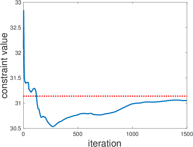
(a) Constraint value $D(\theta_{k})$ in each iteration.

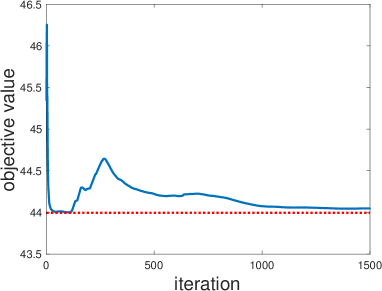
(b) Objective value $J(\theta_{k})$ in each iteration.

Figure 1: An experiment on constrained LQR problem. The iterate starts from an infeasible point and then becomes feasible and eventually converges.

	min value	# iterations	approx. min value	approx. # iterations
Our method	30.689 $\pm$ 0.114	2001 $\pm$ 1172	30.694 $\pm$ 0.114	604.3 $\pm$ 722.4
Lagrangian	30.693 $\pm$ 0.113	7492 $\pm$ 1780	30.699 $\pm$ 0.113	5464 $\pm$ 2116

Table 1: Comparison of our method with Lagrangian method

Appendix A Other applications

A.1 Constrained Parallel Markov Decision Process

We consider the parallel MDP problem [34, 42, 17] where we have a single-agent MDP task and $N$ workers, where each worker acts as an individual agent and aims to solve the same MDP problem. In the parallel MDP setting, each agent is characterized by a tuple $({\mathcal{S}},\mathcal{A},P,\gamma,r^{i},d^{i},\mu^{i})$, where each agent has the same but individual state space, action space, transition probability distribution, and the discount factor. However, the reward function, cost function, and the distribution of the initial state $s_{0}\in{\mathcal{S}}$ could be different for each agent, but satisfy $\mathbb{E}[r^{i}(s,a)]=r(s,a)$, $\mathbb{E}[d^{i}(s,a)]=d(s,a)$, and $\mathbb{E}[\mu^{i}(s,a)]=\mu(s,a)$. Each agent $i$ generates its own trajectory $\{s^{i}_{0},a^{i}_{0},s^{i}_{1},a^{i}_{1},\dots\}$ and collects its own reward/cost value $\{r^{i}_{0},d^{i}_{0},r^{i}_{1},d^{i}_{1},\dots\}$.

The hope is that by solving the single-agent problem using $N$ agents in parallel, the algorithm could be more stable and converge much faster [40]. Intuitively, each agent $i$ may have a different initial state and will explore different parts of the state space due to the randomness in the state transition distribution and the policy. It also helps to reduce the correlation between agents’ behaviors. As a result, by running multiple agents in parallel, we are more likely to visit different parts of the environment and get the experience of the reward/cost function values more efficiently. This mimics the strategy used in tree-based supervised learning algorithms [14, 29, 30].

Following the settings in [17], we have $N$ agents (i.e., $N$ workers) and one central controller in the system. The global parameter is denoted by $\theta$, and we consider the constrained parallel MDP problem where the goal is to solve the following optimization problem:

$$\mathop{\textrm{minimize}}_{\theta}~{}~{}J(\theta)=\sum_{i=1}^{N}\mathbb{E}_{\pi_{\theta}}\biggl{[}-\sum_{t\geq 0}\gamma^{t}\cdot r^{i}(s^{i}_{t},a^{i}_{t})\biggr{]},$$ (28)

$$\text{subject to}~{}~{}D(\theta)=\mathbb{E}_{\pi_{\theta}}\biggl{[}\sum_{t\geq 0}\gamma^{t}\cdot d^{i}(s^{i}_{t},a^{i}_{t})\biggr{]}\leq D_{0},~{}~{}i\in\mathcal{N}.$$

During the estimation step, the controller broadcasts the current parameter $\theta_{k}$ to each agent and each agent samples its own trajectory and obtains estimators for function value/gradient of the reward/cost function. Next, each agent uploads its estimators to the central controller and the central controller takes the average over these estimators, and then follow our proposed algorithm to solve for the QCQP problem and update the parameter to $\theta_{k+1}$. This process continues until convergence.

A.2 Constrained Multi-agent Markov Decision Process

A natural extension of the (single-agent) MDP is to consider a model with $N$ agents termed multi-agent Markov decision process (MMDP). Recently this kind of problem has been attracting more and more attention. See [15] for a comprehensive survey. Most of the work on multi-agent MDP problems consider the setting where the agents share the same global state space, but each with their own collection of actions and rewards [11, 63, 69]. In each stage of the system, each agent observes the global state and chooses its own action individually. As a result, each agent receives its reward and the state evolves according to the joint transition distribution. An MMDP problem can be fully collaborative where all the agents have the same goal, or fully competitive where the problem consists of two agents with an opposite goal, or the mix of the two.

Here we consider a slightly different setting where each agent has its own state space. The only connection between the agents is that the global reward is a function of the overall states and actions. Furthermore, each agent has its own constraint which depends on its own state and action only. This problem is known as Transition-Independent Multi-agent MDP and is considered in [50]. Specifically, each agent’s task is characterized by a tuple $({\mathcal{S}}^{i},\mathcal{A}^{i},P^{i},\gamma,d^{i},\mu^{i})$ with each component defined as usual. Note that $P^{i}\colon{\mathcal{S}}^{i}\times\mathcal{A}^{i}\rightarrow\mathcal{P}({\mathcal{S}}^{i})$ and $d^{i}\colon{\mathcal{S}}^{i}\times\mathcal{A}^{i}\rightarrow\mathbb{R}$ are functions of each agent’s state and action only and do not depend on other agents. Denote ${\mathcal{S}}=\Pi_{i\in\mathcal{N}}{\mathcal{S}}^{i}$ and $\mathcal{A}=\Pi_{i\in\mathcal{N}}\mathcal{A}^{i}$ as the joint state space and action space. The global reward function is given by $r\colon{\mathcal{S}}\times\mathcal{A}\rightarrow\mathbb{R}$ that depends on the joint state and action. Here we consider the fully collaborative setting where all the agents have the same goal. Under this setting, the policy set of each agent is parameterized as $\{\pi^{i}_{\theta^{i}}\colon{\mathcal{S}}^{i}\rightarrow\mathcal{P}(\mathcal{A}^{i})\}$ and we denote $\theta=[\theta^{1},\ldots,\theta^{N}]$ as the overall parameters and $\pi_{\theta}$ as the overall policy. In the following, we use $\mathcal{N}=\{1,2,\ldots,N\}$ to denote the $N$ agents. Denote $a^{i}_{t}$ as the action chosen by agent $i$ at stage $t$ and $a_{t}=\Pi_{i\in\mathcal{N}}~{}a^{i}_{t}$ as the joint action chosen by all the agents. The goal of this constrained MMDP is to solve the following problem

$$\mathop{\textrm{minimize}}_{\theta}~{}~{}J(\theta)=\mathbb{E}_{\pi_{\theta}}\biggl{[}-\sum_{t\geq 0}\gamma^{t}\cdot r(s_{t},a_{t})\biggr{]},$$ (29)

$$\text{subject to}~{}~{}D^{i}(\theta^{i})=\mathbb{E}_{\pi_{\theta^{i}}}\biggl{[}\sum_{t\geq 0}\gamma^{t}\cdot d^{i}(s^{i}_{t},a^{i}_{t})\biggr{]}\leq D^{i}_{0},~{}~{}i\in\mathcal{N}.$$

Inspired by the parallel implementation ([38], Section V), our algorithm applies naturally to constrained MMDP problem with some modifications. This modified procedure can also be viewed as a distributed version of the original algorithm. The overall problem (LABEL:eq:constrained_MMDP) can be viewed as a large “single-agent" problem where the constraints are decomposable into $N$ parts. In this case, instead of solving a large QCQP problem in each iteration, each agent could solve its own QCQP problem in a distributed manner which is much more efficient. As before, we denote the sample negative reward and cost function as

$$J^{*}(\theta)=-\sum_{t\geq 0}\gamma^{t}\cdot r(s_{t},a_{t})\qquad\text{and}\qquad D^{i,*}(\theta^{i})=\sum_{t\geq 0}\gamma^{t}\cdot d^{i}(s^{i}_{t},a^{i}_{t}).$$

In each iteration with $\theta_{k}=[\theta^{1}_{k},...,\theta^{N}_{k}]$, we approximate $J(\theta)$ and $D(\theta)$ as

$$\widetilde{J}^{i}(\theta^{i},\theta_{k},\tau) =\frac{1}{N}J^{*}(\theta_{k})+\langle\nabla_{\theta^{i}}J^{*}(\theta_{k}),\theta^{i}-\theta^{i}_{k}\rangle+\tau\|\theta^{i}-\theta^{i}_{k}\|_{2}^{2},$$ (30)

$$\widetilde{D}^{i}(\theta^{i},\theta_{k},\tau) =D^{i,*}(\theta^{i}_{k})+\langle\nabla_{\theta^{i}}D^{i,*}(\theta^{i}_{k}),\theta^{i}-\theta^{i}_{k}\rangle+\tau\|\theta^{i}-\theta^{i}_{k}\|_{2}^{2}.$$ (31)

Note that the constraint function is naturally decomposable into $N$ parts. We also “manually" split the objective function into $N$ parts, so that each agent could solve its own QCQP problem in a distributed manner. As before, we define

$$\overline{J}^{i,(k)}(\theta^{i})=(1-\rho_{k})\cdot\overline{J}^{i,(k-1)}(\theta^{i})+\rho_{k}\cdot\widetilde{J}^{i}(\theta^{i},\theta_{k},\tau),$$

$$\overline{D}^{i,(k)}(\theta^{i})=(1-\rho_{k})\cdot\overline{D}^{i,(k-1)}(\theta^{i})+\rho_{k}\cdot\widetilde{D}^{i}(\theta^{i},\theta_{k},\tau).$$

With this surrogate functions, each agent then solves its own convex relaxation problem

$$\overline{\theta}^{i}_{k}=\mathop{\mathrm{argmin}}_{\theta^{i}}~{}\overline{J}^{i,(k)}(\theta^{i})\qquad\text{subject to}\qquad\overline{D}^{i,(k)}(\theta^{i})\leq D^{i}_{0},$$ (32)

or, alternatively, solves for the feasibility problem if (32) is infeasible

$$\overline{\theta}^{i}_{k}=\mathop{\mathrm{argmin}}_{\theta^{i},\alpha^{i}}~{}\alpha^{i}\qquad\text{subject to}\qquad\overline{D}^{i,(k)}(\theta^{i})\leq D^{i}_{0}+\alpha^{i}.$$ (33)

This step can be implemented in a distributed manner for each agent and is more efficient than solving the overall problem with the overall parameter $\theta$. Finally, the update rule for each agent $i$ is as usual

$$\theta^{i}_{t+1}=(1-\eta_{k})\cdot\theta^{i}_{k}+\eta_{k}\cdot\overline{\theta}^{i}_{k}.$$

This process continues until convergence.

Appendix B Proof of Theorem 4

According to the choice of the surrogate function (9) and Assumption 2, it is straightforward to verify that the function $\overline{J}^{(k)}(\theta)$ defined in (12) is uniformly strongly convex in $\theta$ for each iteration $t$. Moreover, both $\overline{J}^{(k)}(\theta)$ and $\nabla_{\theta}\overline{J}^{(k)}(\theta)$ are Lipschitz continuous functions.

From Lemma 1 in [49] we have

$$\lim_{t\to\infty}\Big{|}\overline{J}^{(k)}(\theta)-\mathbb{E}\big{[}\widetilde{J}(\theta,\theta_{k},\tau)\big{]}\Big{|}=0.$$

Since the function $\mathbb{E}\big{[}\widetilde{J}(\theta,\theta_{k},\tau)\big{]}$ is Lipschitz continuous in $\theta_{k}$, we obtain that

$$\Big{|}\overline{J}^{(k_{1})}(\theta)-\overline{J}^{(k_{2})}(\theta)\Big{|}\leq L_{0}\cdot\|\theta_{k_{1}}-\theta_{k_{2}}\|+\epsilon,$$

for some constant $L_{0}$ and the error term $\epsilon$ that goes to $0$ as $k_{1},k_{2}$ go to infinity. This shows that the function sequence $\overline{J}^{(k_{j})}(\theta)$ is equicontinuous. Since $\Theta$ is compact and the discounted cumulative reward function is bounded by $r_{\max}/(1-\gamma)$, we can apply Arzela-Ascoli theorem [22, 32] to prove existence of $\widehat{J}(\theta)$ that converges uniformly. Moreover, since we apply the same operations on the constraint function $D(\theta)$ as to the reward function $J(\theta)$ in Algorithm 1, the above properties also hold for $D(\theta)$.

The rest of the proof follows in a similar way as the proof of Theorem 1 in [38]. Under Assumptions 1 - 3, the technical conditions in [38] are satisfied by the choice of the surrogate functions (9) and (10). According to Lemma 2 in [38], with probability one we have

$$\mathop{\lim\sup}_{k\to\infty}D(\theta_{k})\leq D_{0}.$$

This shows that, although in some of the iterations the convex relaxation problem (11) is infeasible, and we have to solve the alternative problem (14), the iterates $\{\theta_{k}\}$ converge to the feasible region of the original problem (LABEL:eq:constrained) with probability one. Furthermore, with probability one, the convergent point $\widetilde{\theta}$ is the optimal solution to the following problem

$$\mathop{\textrm{minimize}}_{\theta\in\Theta}~{}~{}\widehat{J}(\theta)\qquad\text{subject to}\qquad\widehat{D}(\theta)\leq D_{0}.$$ (34)

The KKT conditions for (34) together with the Slater condition show that the KKT conditions of the original problem (LABEL:eq:constrained) are also satisfied at $\widetilde{\theta}$. This shows that $\widetilde{\theta}$ is a stationary point of the original problem almost surely.

References

- [1] Joshua Achiam, David Held, Aviv Tamar, and Pieter Abbeel. Constrained policy optimization. In International Conference on Machine Learning, pages 22–31, 2017.
- [2] Leonard Adolphs. Non convex-concave saddle point optimization. Master’s thesis, ETH Zurich, 2018.
- [3] Eitan Altman. Constrained Markov decision processes, volume 7. CRC Press, 1999.
- [4] Haitham Bou Ammar, Rasul Tutunov, and Eric Eaton. Safe policy search for lifelong reinforcement learning with sublinear regret. In International Conference on Machine Learning, pages 2361–2369, 2015.
- [5] Dario Amodei, Chris Olah, Jacob Steinhardt, Paul Christiano, John Schulman, and Dan Mané. Concrete problems in ai safety. arXiv preprint arXiv:1606.06565, 2016.
- [6] Brian DO Anderson and John B Moore. Optimal control: linear quadratic methods. Courier Corporation, 2007.
- [7] Yu Bai, Tengyang Xie, Nan Jiang, and Yu-Xiang Wang. Provably efficient q-learning with low switching cost. arXiv preprint arXiv:1905.12849, 2019.
- [8] Marc G Bellemare, Yavar Naddaf, Joel Veness, and Michael Bowling. The arcade learning environment: An evaluation platform for general agents. Journal of Artificial Intelligence Research, 47:253–279, 2013.
- [9] Felix Berkenkamp, Matteo Turchetta, Angela Schoellig, and Andreas Krause. Safe model-based reinforcement learning with stability guarantees. In Advances in Neural Information Processing Systems, pages 908–918, 2017.
- [10] Vivek S Borkar. Stochastic approximation with two time scales. Systems & Control Letters, 29(5):291–294, 1997.
- [11] Craig Boutilier. Planning, learning and coordination in multiagent decision processes. In Proceedings of the 6th conference on Theoretical aspects of rationality and knowledge, pages 195–210. Morgan Kaufmann Publishers Inc., 1996.
- [12] Steven J Bradtke. Reinforcement learning applied to linear quadratic regulation. In Advances in neural information processing systems, pages 295–302, 1993.
- [13] Steven J Bradtke, B Erik Ydstie, and Andrew G Barto. Adaptive linear quadratic control using policy iteration. In Proceedings of the American control conference, volume 3, pages 3475–3475. Citeseer, 1994.
- [14] Leo Breiman. Random forests. Machine learning, 45(1):5–32, 2001.
- [15] Lucian Busoniu, Robert Babuska, and Bart De Schutter. A comprehensive survey of multiagent reinforcement learning. IEEE Transactions on Systems, Man, And Cybernetics-Part C: Applications and Reviews, 38 (2), 2008, 2008.
- [16] Qi Cai, Zhuoran Yang, Jason D Lee, and Zhaoran Wang. Neural temporal-difference learning converges to global optima. arXiv preprint arXiv:1905.10027, 2019.
- [17] Tianyi Chen, Kaiqing Zhang, Georgios B Giannakis, and Tamer Başar. Communication-efficient distributed reinforcement learning. arXiv preprint arXiv:1812.03239, 2018.
- [18] Yinlam Chow, Mohammad Ghavamzadeh, Lucas Janson, and Marco Pavone. Risk-constrained reinforcement learning with percentile risk criteria. Journal of Machine Learning Research, 18(167):1–167, 2017.
- [19] Yinlam Chow, Ofir Nachum, Edgar Duenez-Guzman, and Mohammad Ghavamzadeh. A lyapunov-based approach to safe reinforcement learning. arXiv preprint arXiv:1805.07708, 2018.
- [20] Christoph Dann, Gerhard Neumann, and Jan Peters. Policy evaluation with temporal differences: A survey and comparison. The Journal of Machine Learning Research, 15(1):809–883, 2014.
- [21] Sarah Dean, Horia Mania, Nikolai Matni, Benjamin Recht, and Stephen Tu. On the sample complexity of the linear quadratic regulator. arXiv preprint arXiv:1710.01688, 2017.
- [22] Nelson Dunford and Jacob T Schwartz. Linear operators part I: general theory, volume 7. Interscience publishers New York, 1958.
- [23] Lawrence C Evans. An introduction to mathematical optimal control theory. Lecture Notes, University of California, Department of Mathematics, Berkeley, 2005.
- [24] Maryam Fazel, Rong Ge, Sham Kakade, and Mehran Mesbahi. Global convergence of policy gradient methods for the linear quadratic regulator. In International Conference on Machine Learning, pages 1466–1475, 2018.
- [25] Jaime F Fisac, Anayo K Akametalu, Melanie N Zeilinger, Shahab Kaynama, Jeremy Gillula, and Claire J Tomlin. A general safety framework for learning-based control in uncertain robotic systems. IEEE Transactions on Automatic Control, 2018.
- [26] Javier Garcıa and Fernando Fernández. A comprehensive survey on safe reinforcement learning. Journal of Machine Learning Research, 16(1):1437–1480, 2015.
- [27] Ian Goodfellow, Jean Pouget-Abadie, Mehdi Mirza, Bing Xu, David Warde-Farley, Sherjil Ozair, Aaron Courville, and Yoshua Bengio. Generative adversarial nets. In Advances in neural information processing systems, pages 2672–2680, 2014.
- [28] Ivo Grondman, Lucian Busoniu, Gabriel AD Lopes, and Robert Babuska. A survey of actor-critic reinforcement learning: Standard and natural policy gradients. IEEE Transactions on Systems, Man, and Cybernetics, Part C (Applications and Reviews), 42(6):1291–1307, 2012.
- [29] Jingyu He, Saar Yalov, and P Richard Hahn. XBART: Accelerated Bayesian additive regression trees. In The 22nd International Conference on Artificial Intelligence and Statistics, pages 1130–1138, 2019.
- [30] Jingyu He, Saar Yalov, Jared Murray, and P Richard Hahn. Stochastic tree ensembles for regularized supervised learning. Technical report, 2019.
- [31] Jessie Huang, Fa Wu, Doina Precup, and Yang Cai. Learning safe policies with expert guidance. arXiv preprint arXiv:1805.08313, 2018.
- [32] John L Kelley. General topology. Courier Dover Publications, 2017.
- [33] Vijay R Konda and John N Tsitsiklis. Actor-critic algorithms. In Advances in neural information processing systems, pages 1008–1014, 2000.
- [34] R Matthew Kretchmar. Parallel reinforcement learning. In The 6th World Conference on Systemics, Cybernetics, and Informatics. Citeseer, 2002.
- [35] Jonathan Lacotte, Yinlam Chow, Mohammad Ghavamzadeh, and Marco Pavone. Risk-sensitive generative adversarial imitation learning. arXiv preprint arXiv:1808.04468, 2018.
- [36] Dennis Lee, Haoran Tang, Jeffrey O Zhang, Huazhe Xu, Trevor Darrell, and Pieter Abbeel. Modular architecture for starcraft ii with deep reinforcement learning. In Fourteenth Artificial Intelligence and Interactive Digital Entertainment Conference, 2018.
- [37] Yuxi Li. Deep reinforcement learning: An overview. arXiv preprint arXiv:1701.07274, 2017.
- [38] An Liu, Vincent Lau, and Borna Kananian. Stochastic successive convex approximation for non-convex constrained stochastic optimization. arXiv preprint arXiv:1801.08266, 2018.
- [39] Boyi Liu, Qi Cai, Zhuoran Yang, and Zhaoran Wang. Neural proximal/trust region policy optimization attains globally optimal policy. arXiv preprint arXiv:1906.10306, 2019.
- [40] Volodymyr Mnih, Adria Puigdomenech Badia, Mehdi Mirza, Alex Graves, Timothy Lillicrap, Tim Harley, David Silver, and Koray Kavukcuoglu. Asynchronous methods for deep reinforcement learning. In International conference on machine learning, pages 1928–1937, 2016.
- [41] Volodymyr Mnih, Koray Kavukcuoglu, David Silver, Andrei A Rusu, Joel Veness, Marc G Bellemare, Alex Graves, Martin Riedmiller, Andreas K Fidjeland, Georg Ostrovski, et al. Human-level control through deep reinforcement learning. Nature, 518(7540):529, 2015.
- [42] Arun Nair, Praveen Srinivasan, Sam Blackwell, Cagdas Alcicek, Rory Fearon, Alessandro De Maria, Vedavyas Panneershelvam, Mustafa Suleyman, Charles Beattie, Stig Petersen, et al. Massively parallel methods for deep reinforcement learning. arXiv preprint arXiv:1507.04296, 2015.
- [43] Santiago Paternain. Stochastic Control Foundations of Autonomous Behavior. PhD thesis, University of Pennsylvania, 2018.
- [44] Peng Peng, Ying Wen, Yaodong Yang, Quan Yuan, Zhenkun Tang, Haitao Long, and Jun Wang. Multiagent bidirectionally-coordinated nets: Emergence of human-level coordination in learning to play starcraft combat games. arXiv preprint arXiv:1703.10069, 2017.
- [45] Matteo Pirotta, Marcello Restelli, and Luca Bascetta. Policy gradient in lipschitz markov decision processes. Machine Learning, 100(2-3):255–283, 2015.
- [46] LA Prashanth and Mohammad Ghavamzadeh. Variance-constrained actor-critic algorithms for discounted and average reward mdps. Machine Learning, 105(3):367–417, 2016.
- [47] Benjamin Recht. A tour of reinforcement learning: The view from continuous control. Annual Review of Control, Robotics, and Autonomous Systems, 2018.
- [48] Chang-han Rhee and Peter W Glynn. Unbiased estimation with square root convergence for sde models. Operations Research, 63(5):1026–1043, 2015.
- [49] Andrzej Ruszczyński. Feasible direction methods for stochastic programming problems. Mathematical Programming, 19(1):220–229, 1980.
- [50] Joris Scharpff, Diederik M Roijers, Frans A Oliehoek, Matthijs TJ Spaan, and Mathijs Michiel de Weerdt. Solving transition-independent multi-agent mdps with sparse interactions. In AAAI, pages 3174–3180, 2016.
- [51] John Schulman, Sergey Levine, Pieter Abbeel, Michael Jordan, and Philipp Moritz. Trust region policy optimization. In International Conference on Machine Learning, pages 1889–1897, 2015.
- [52] Gesualdo Scutari, Francisco Facchinei, Peiran Song, Daniel P Palomar, and Jong-Shi Pang. Decomposition by partial linearization: Parallel optimization of multi-agent systems. IEEE Transactions on Signal Processing, 62(3):641–656, 2013.
- [53] David Silver, Aja Huang, Chris J Maddison, Arthur Guez, Laurent Sifre, George Van Den Driessche, Julian Schrittwieser, Ioannis Antonoglou, Veda Panneershelvam, Marc Lanctot, et al. Mastering the game of go with deep neural networks and tree search. nature, 529(7587):484, 2016.
- [54] David Silver, Thomas Hubert, Julian Schrittwieser, Ioannis Antonoglou, Matthew Lai, Arthur Guez, Marc Lanctot, Laurent Sifre, Dharshan Kumaran, Thore Graepel, et al. A general reinforcement learning algorithm that masters chess, shogi, and go through self-play. Science, 362(6419):1140–1144, 2018.
- [55] David Silver, Julian Schrittwieser, Karen Simonyan, Ioannis Antonoglou, Aja Huang, Arthur Guez, Thomas Hubert, Lucas Baker, Matthew Lai, Adrian Bolton, et al. Mastering the game of go without human knowledge. Nature, 550(7676):354, 2017.
- [56] Peng Sun, Xinghai Sun, Lei Han, Jiechao Xiong, Qing Wang, Bo Li, Yang Zheng, Ji Liu, Yongsheng Liu, Han Liu, et al. Tstarbots: Defeating the cheating level builtin ai in starcraft ii in the full game. arXiv preprint arXiv:1809.07193, 2018.
- [57] Ying Sun, Prabhu Babu, and Daniel P Palomar. Majorization-minimization algorithms in signal processing, communications, and machine learning. IEEE Transactions on Signal Processing, 65(3):794–816, 2016.
- [58] Richard S Sutton and Andrew G Barto. Reinforcement learning: An introduction. MIT press, 2018.
- [59] Richard S Sutton, David A McAllester, Satinder P Singh, and Yishay Mansour. Policy gradient methods for reinforcement learning with function approximation. In Advances in neural information processing systems, pages 1057–1063, 2000.
- [60] Chen Tessler, Daniel J Mankowitz, and Shie Mannor. Reward constrained policy optimization. arXiv preprint arXiv:1805.11074, 2018.
- [61] Matteo Turchetta, Felix Berkenkamp, and Andreas Krause. Safe exploration in finite markov decision processes with gaussian processes. In Advances in Neural Information Processing Systems, pages 4312–4320, 2016.
- [62] Oriol Vinyals, Timo Ewalds, Sergey Bartunov, Petko Georgiev, Alexander Sasha Vezhnevets, Michelle Yeo, Alireza Makhzani, Heinrich Küttler, John Agapiou, Julian Schrittwieser, et al. Starcraft ii: A new challenge for reinforcement learning. arXiv preprint arXiv:1708.04782, 2017.
- [63] Hoi-To Wai, Zhuoran Yang, Zhaoran Wang, and Mingyi Hong. Multi-agent reinforcement learning via double averaging primal-dual optimization. arXiv preprint arXiv:1806.00877, 2018.
- [64] Lingxiao Wang, Qi Cai, Zhuoran Yang, and Zhaoran Wang. Neural policy gradient methods: Global optimality and rates of convergence. arXiv preprint arXiv:1909.01150, 2019.
- [65] Min Wen and Ufuk Topcu. Constrained cross-entropy method for safe reinforcement learning. In Advances in Neural Information Processing Systems, pages 7461–7471, 2018.
- [66] Sijia Xu, Hongyu Kuang, Zhi Zhuang, Renjie Hu, Yang Liu, and Huyang Sun. Macro action selection with deep reinforcement learning in starcraft. arXiv preprint arXiv:1812.00336, 2018.
- [67] Yang Yang, Gesualdo Scutari, Daniel P Palomar, and Marius Pesavento. A parallel decomposition method for nonconvex stochastic multi-agent optimization problems. IEEE Transactions on Signal Processing, 64(11):2949–2964, 2016.
- [68] Zhuoran Yang, Yongxin Chen, Mingyi Hong, and Zhaoran Wang. On the global convergence of actor-critic: A case for linear quadratic regulator with ergodic cost. arXiv preprint arXiv:1907.06246, 2019.
- [69] Kaiqing Zhang, Zhuoran Yang, Han Liu, Tong Zhang, and Tamer Başar. Finite-sample analyses for fully decentralized multi-agent reinforcement learning. arXiv preprint arXiv:1812.02783, 2018.