Pseudospectra of Loewner Matrix Pencils

Abstract

Loewner matrix pencils play a central role in the system realization theory of Mayo and Antoulas, an important development in data-driven modeling. The eigenvalues of these pencils reveal system poles. How robust are the poles recovered via Loewner realization? With several simple examples, we show how pseudospectra of Loewner pencils can be used to investigate the influence of interpolation point location and partitioning on pole stability, the transient behavior of the realized system, and the effect of noisy measurement data. We include an algorithm to efficiently compute such pseudospectra by exploiting Loewner structure.

Dedicated to Thanos Antoulas.

1 Introduction

The landmark systems realization theory of Mayo and Antoulas MA07 constructs a dynamical system that interpolates tangential frequency domain measurements of a multi-input, multi-output system. Central to this development is the matrix pencil $z{\rm I\kern-1.25ptL}-{\rm I\kern-1.25ptL}_{s}$ composed of Loewner and shifted Loewner matrices ${\rm I\kern-1.25ptL}$ and ${\rm I\kern-1.25ptL}_{s}$ that encode the interpolation data. When this technique is used for exact system recovery (as opposed to data-driven model reduction), the eigenvalues of this pencil match the poles of the original dynamical system. However other spectral properties, including the sensitivity of the eigenvalues to perturbation, can differ significantly; indeed, they depend upon the location of the interpolation points in the complex plane relative to the system poles, and how the poles are partitioned. Since in many scenarios one uses $z{\rm I\kern-1.25ptL}-{\rm I\kern-1.25ptL}_{s}$ to learn about the original system, such subtle differences matter.

Pseudospectra are sets in the complex plane that contain the eigenvalues but provide additional insight about the sensitivity of those eigenvalues to perturbation and the transient behavior of the underlying dynamical system. While most often used to analyze single matrices, pseudospectral concepts have been extended to matrix pencils (generalized eigenvalue problems).

This introductory note shows several ways to use pseudospectra to investigate spectral questions involving Loewner pencils derived from system realization problems. Using simple examples, we explore the following questions.

• How do the locations of the interpolation points and their partition into “left” and “right” points affect the sensitivity of the eigenvalues of $z{\rm I\kern-1.25ptL}-{\rm I\kern-1.25ptL}_{s}$?

• Do solutions to the dynamical system ${\rm I\kern-1.25ptL}\dot{\bf x}(t)={\rm I\kern-1.25ptL}_{s}{\bf x}(t)$ mimic solutions to the original system $\dot{\bf x}(t)={\bf A}{\bf x}(t)$, especially in the transient regime? Does this agreement depend on the interpolation points?

• How do noisy measurements affect the eigenvalues of $z{\rm I\kern-1.25ptL}-{\rm I\kern-1.25ptL}_{s}$?

We include an algorithm for computing pseudospectra of an $n$-dimensional Loewner pencil in ${\cal O}(n^{2})$ operations, improving the ${\cal O}(n^{3})$ cost for generic matrix pencils; the appendix gives a MATLAB implementation.

Throughout this note, we use $\sigma(\cdot)$ to denote the spectrum (eigenvalues) of a matrix or matrix pencil, and $\|\cdot\|$ to denote the vector 2-norm and the matrix norm it induces. (All definitions here can readily be adapted to other norms, as needed. The algorithm, however, is designed for use with the 2-norm.)

2 Loewner realization theory in a nutshell

We briefly summarize Loewner realization theory, as developed by Mayo and Antoulas MA07 ; see also ALI17 . Consider the linear, time-invariant dynamical system

$${\bf E}\dot{\bf x}(t) = {\bf A}{\bf x}(t)+{\bf B}{\bf u}(t)$$

$${\bf y}(t) = {\bf C}{\bf x}(t)$$

for ${\bf A},{\bf E}\in\mathbbm{C}^{n\times n}$, ${\bf B}\in\mathbbm{C}^{n\times m}$, and ${\bf C}\in\mathbbm{C}^{p\times n}$, with which we associate, via the Laplace transform, the transfer function ${\bf H}(z)={\bf C}(z{\bf E}-{\bf A})^{-1}{\bf B}$.

Given tangential measurements of ${\bf H}(z)$ we seek to build a realization of the system that interpolates the given data. More precisely, consider the right interpolation data
       $\bullet$ distinct interpolation points $\lambda_{1},\ldots,\lambda_{\varrho}\in\mathbbm{C}$;
       $\bullet$ interpolation directions ${\bf r}_{1},\ldots,{\bf r}_{\varrho}\in\mathbbm{C}^{m}$;
       $\bullet$ function values ${\bf w}_{1},\ldots,{\bf w}_{\varrho}\in\mathbbm{C}^{p}$;
and left interpolation data
       $\bullet$ distinct interpolation points $\mu_{1},\ldots,\mu_{\nu}\in\mathbbm{C}$;
       $\bullet$ interpolation directions $\boldsymbol{\ell}_{1},\ldots,\boldsymbol{\ell}_{\nu}\in\mathbbm{C}^{p}$;
       $\bullet$ function values ${\bf v}_{1},\ldots,{\bf v}_{\nu}\in\mathbbm{C}^{m}$.
Assume the left and right interpolation points are disjoint $\{\lambda_{i}\}_{i=1}^{\varrho}\cap\{\mu_{j}\}_{j=1}^{\nu}=\emptyset$; indeed in our examples we will consider all the left and right points to be distinct.

The interpolation problem seeks matrices $\widehat{{\bf A}},\widehat{{\bf E}},\widehat{{\bf B}},\widehat{{\bf C}}$ for which the transfer function $\widehat{{\bf H}}(z)=\widehat{{\bf C}}(z\widehat{{\bf E}}-\widehat{{\bf A}})^{-1}\widehat{{\bf B}}$ interpolates the data: for $i=1,\ldots,\varrho$ and $j=1,\ldots,\nu$,

$$\widehat{{\bf H}}(\lambda_{i}){\bf r}_{i}={\bf w}_{i},\qquad\boldsymbol{\ell}_{j}^{*}\widehat{{\bf H}}(\mu_{j})={\bf v}_{j}^{*}.$$

Two structured matrices play a crucial role in the development of Mayo and Antoulas MA07 . From the data, construct the Loewner and shifted Loewner matrices

$${\rm I\kern-1.25ptL}=\left[\begin{array}[]{ccc}{{\bf v}_{1}^{*}{\bf r}_{1}-\boldsymbol{\ell}_{1}^{*}{\bf w}_{1}\over\mu_{1}-\lambda_{1}}&\cdots&{{\bf v}_{1}^{*}{\bf r}_{\varrho}-\boldsymbol{\ell}_{1}^{*}{\bf w}_{\varrho}\over\mu_{1}-\lambda_{\varrho}}\\ \vdots&\ddots&\vdots\\ {{\bf v}_{\nu}^{*}{\bf r}_{1}-\boldsymbol{\ell}_{\nu}^{*}{\bf w}_{1}\over\mu_{\nu}-\lambda_{1}}&\cdots&{{\bf v}_{\nu}^{*}{\bf r}_{\varrho}-\boldsymbol{\ell}_{\nu}^{*}{\bf w}_{\varrho}\over\mu_{\nu}-\lambda_{\varrho}}\\ \end{array}\right],\quad{\rm I\kern-1.25ptL}_{s}=\left[\begin{array}[]{ccc}{\mu_{1}{\bf v}_{1}^{*}{\bf r}_{1}-\lambda_{1}\boldsymbol{\ell}_{1}^{*}{\bf w}_{1}\over\mu_{1}-\lambda_{1}}&\cdots&{\mu_{1}{\bf v}_{1}^{*}{\bf r}_{\varrho}-\lambda_{\varrho}\boldsymbol{\ell}_{1}^{*}{\bf w}_{\varrho}\over\mu_{1}-\lambda_{\varrho}}\\ \vdots&\ddots&\vdots\\ {\mu_{\nu}{\bf v}_{\nu}^{*}{\bf r}_{1}-\lambda_{1}\boldsymbol{\ell}_{\nu}^{*}{\bf w}_{1}\over\mu_{\nu}-\lambda_{1}}&\cdots&{\mu_{\nu}{\bf v}_{\nu}^{*}{\bf r}_{\varrho}-\lambda_{\varrho}\boldsymbol{\ell}_{\nu}^{*}{\bf w}_{\varrho}\over\mu_{\nu}-\lambda_{\varrho}}\\ \end{array}\right]$$ (1)

i.e., the $(i,j)$ entries of these $\nu\times\varrho$ matrices have the form

$$({\rm I\kern-1.25ptL})_{i,j}={{\bf v}_{i}^{*}{\bf r}_{j}-\boldsymbol{\ell}_{i}^{*}{\bf w}_{j}\over\mu_{i}-\lambda_{j}},\qquad({{\rm I\kern-1.25ptL}_{s}})_{i,j}={\mu_{i}{\bf v}_{i}^{*}{\bf r}_{j}-\lambda_{j}\boldsymbol{\ell}_{i}^{*}{\bf w}_{j}\over\mu_{i}-\lambda_{j}}.$$

Now collect the data into matrices. The right interpolation points, directions, and data are stored in

$$\mbox{\boldmath$\Lambda$}=\left[\begin{array}[]{ccc}\lambda_{1}\\ &\ddots\\ &&\lambda_{\varrho}\end{array}\right]\!\in\!\mathbbm{C}^{\varrho\times\varrho},\quad{\bf R}=\left[\begin{array}[]{ccc}\\ {\bf r}_{1}&\cdots{\bf r}_{\varrho}\\ &\end{array}\right]\!\in\!\mathbbm{C}^{m\times\varrho},\quad{\bf W}=\left[\begin{array}[]{ccc}\\ {\bf w}_{1}&\cdots{\bf w}_{\varrho}\\ &\end{array}\right]\!\in\!\mathbbm{C}^{p\times\varrho},$$

while the left interpolation points, directions, and data are stored in

$${\bf M}=\left[\begin{array}[]{ccc}\mu_{1}\\ &\ddots\\ &&\mu_{\nu}\end{array}\right]\!\in\!\mathbbm{C}^{\nu\times\nu},\quad{\bf L}=\left[\begin{array}[]{ccc}\\ \boldsymbol{\ell}_{1}&\cdots\boldsymbol{\ell}_{\nu}\\ &\end{array}\right]\!\in\!\mathbbm{C}^{p\times\nu},\quad{\bf V}=\left[\begin{array}[]{ccc}\\ {\bf v}_{1}&\cdots{\bf v}_{\nu}\\ &\end{array}\right]\!\in\!\mathbbm{C}^{m\times\nu}.$$

2.1 Selecting and arranging interpolation points

As Mayo and Antoulas observe, Sylvester equations connect these matrices:

$${\rm I\kern-1.25ptL}\mbox{\boldmath$\Lambda$}-{\bf M}{\rm I\kern-1.25ptL}={\bf L}^{*}{\bf W}-{\bf V}^{*}{\bf R},\qquad{\rm I\kern-1.25ptL}_{s}\mbox{\boldmath$\Lambda$}-{\bf M}{\rm I\kern-1.25ptL}_{s}={\bf L}^{*}{\bf W}\mbox{\boldmath$\Lambda$}-{\bf M}{\bf V}^{*}{\bf R}.$$ (2)

Just using the dimensions of the components, note that

$${\rm rank}({\bf L}^{*}{\bf W}),\ {\rm rank}({\bf V}^{*}{\bf R}),\ {\rm rank}({\bf L}^{*}{\bf W}\mbox{\boldmath$\Lambda$}),\ {\rm rank}({\bf V}^{*}{\bf R}{\bf M})\leq\min\{\nu,\varrho,m,p\}.$$

Thus for modest $m$ and $p$, the Sylvester equations (2) must have low-rank right-hand sides. This situation often implies the rapid decay of singular values of solutions to the Sylvester equation ASZ02 ; BT17 ; Pen00a ; Pen00b ; Sab06 . While this phenomenon is convenient in the context of balanced truncation model reduction (enabling low-rank approximations to the controllability and observability Gramians), it is less welcome in the Loewner realization setting, where the rank of ${\rm I\kern-1.25ptL}$ should reveal the order of the original system: fast decay of the singular values of ${\rm I\kern-1.25ptL}$ makes this rank ambiguous. Since $\Lambda$ and ${\bf M}$ are diagonal, they are normal matrices, and hence Theorem 2.1 of BT17 gives

$$\frac{s_{qk+1}({\rm I\kern-1.25ptL})}{s_{1}({\rm I\kern-1.25ptL})}\leq\inf_{\phi\in{\cal R}_{k,k}}\frac{\max\{|\phi(\lambda)|:\lambda\in\{\lambda_{1},\ldots,\lambda_{\varrho}\}\}}{\min\{|\phi(\mu)|:\mu\in\{\mu_{1},\ldots,\mu_{\nu}\}\}},$$ (3)

where $s_{j}(\cdot)$ denotes the $j$th largest singular value, $q={\rm rank}({\bf L}^{*}{\bf W}-{\bf V}^{*}{\bf R})$, and ${\cal R}_{k,k}$ denotes the set of irreducible rational functions whose numerators and denominators are polynomials of degree $k$ or less. The right hand side of (3) will be small when there exists some $\phi\in{\cal R}_{k,k}$ for which all $|\phi(\lambda_{i})|$ are small, while all $|\phi(\mu_{j})|$ are large: a good separation of $\{\lambda_{i}\}$ from $\{\mu_{j}\}$ is thus sufficient to ensure the rapid decay of the singular values of ${\rm I\kern-1.25ptL}$ and ${\rm I\kern-1.25ptL}_{s}$. (Beckermann and Townsend give an explicit bound for the singular values of Loewner matrices when the interpolation points fall in disjoint real intervals (BT17, , Cor. 4.2).)

In our setting, where we want the singular values of ${\rm I\kern-1.25ptL}$ and ${\rm I\kern-1.25ptL}_{s}$ to reveal the system’s order (without artificial decay of singular values as an accident of the arrangement of interpolation points), it is necessary for one $|\phi(\lambda_{i})|$ to be at least the same size as the smallest value of $|\phi(\mu_{j})|$ for all $\phi\in{\cal R}_{k,k}$. Roughly speaking, we want the left and right interpolation points to be close together (even interleaved). While this arrangement is necessary for slow decay of the singular values, it does not alone prevent such decay, as evident in Figure 4 (since (3) is only an upper bound).

Another heuristic, based on the Cauchy-like structure of ${\rm I\kern-1.25ptL}$ and ${\rm I\kern-1.25ptL}_{s}$, also suggests the left and right interpolation points should be close together. Namely, ${\rm I\kern-1.25ptL}$ and ${\rm I\kern-1.25ptL}_{s}$ are a more general form of the Cauchy matrix $({\boldsymbol{\mathcal{C}}})_{i,j}=1/(\mu_{i}-\lambda_{j})$, whose determinant has the elegant formula (e.g., (HJ13, , p. 38))

$${\rm det}({\boldsymbol{\mathcal{C}}})=\frac{\prod_{1\leq i<j\leq n}(\mu_{j}-\mu_{i})(\lambda_{i}-\lambda_{j})}{\prod_{1\leq i\leq j\leq n}(\mu_{i}-\lambda_{j})}.$$ (4)

It is an open question if ${\rm det}({\rm I\kern-1.25ptL})$ and ${\rm det}({\rm I\kern-1.25ptL}_{s})$ have similarly elegant formulas. Nevertheless, ${\rm det}({\rm I\kern-1.25ptL})$ and ${\rm det}({\rm I\kern-1.25ptL}_{s})$ do have the same denominator as ${\rm det}({\boldsymbol{\mathcal{C}}})$ (which can be checked by recursively subtracting the first row from all other rows when computing the determinant). This observation suggests that to avoid artificially small determinants for ${\rm I\kern-1.25ptL}$ and ${\rm I\kern-1.25ptL}_{s}$ (which, up to sign, are the products of the singular values) it is necessary for the denominator of (4) to be small, and, thus, for the left and right interpolation points to be close together.

In practice, we often start with initial interpolation points $x_{1},\ldots,x_{2n}$ that we want to partition into left and right interpolation points to form ${\rm I\kern-1.25ptL}$ and ${\rm I\kern-1.25ptL}_{s}$. Our analysis of (4) suggests a simple way to arrange the interpolation points such that the denominator of ${\rm det}({\rm I\kern-1.25ptL})$ and ${\rm det}({\rm I\kern-1.25ptL}_{s})$ is small: relabel the points to satisfy

$$x_{k}=\underset{k\leq q\leq 2n}{\arg\min}~{}|x_{k-1}-x_{q}|,\quad{\rm for}~{}~{}k=2,\ldots,2n,$$ (5)

$$\{\mu_{i}\}=\{x_{1},x_{3},\ldots,x_{2n-1}\},\quad\{\lambda_{j}\}=\{x_{2},x_{4},\ldots,x_{2n}\}.$$

The greedy reordering in (5) ensures that $|x_{k}-x_{k-1}|$ is small and allows us to simply interleave the left and right interpolation points. Moreover, when $x_{1},\ldots,x_{2n}$ are located on a line, the reordering in (5) simplifies to directly interleaving $\mu_{i}$ and $\lambda_{j}$ and, thus, it can be skipped. This ordering need not be optimal, as we do not visit all possible combinations of $\mu_{i}-\lambda_{j}$; it simply seeks a partition that yields a large determinant (which must also depend on the interpolation data). We note its simplicity, effectiveness, and efficiency (requiring only ${\cal O}(n^{2})$ operations).

2.2 Construction of interpolants

Throughout we make the fundamental assumptions that for all $\widehat{z}\in\{\lambda_{i}\}_{i=1}^{\varrho}\cup\{\mu_{j}\}_{j=1}^{\nu}$,

$${\rm rank}\mkern 1.0mu(\widehat{z}\mkern 1.0mu\mkern 1.0mu\mkern 1.0mu{\rm I\kern-1.25ptL}-{\rm I\kern-1.25ptL}_{s})={\rm rank}\left(\left[\begin{array}[]{c}{\rm I\kern-1.25ptL}\\ {\rm I\kern-1.25ptL}_{s}\end{array}\right]\right)={\rm rank}\left(\left[\begin{array}[]{cc}{\rm I\kern-1.25ptL}&{\rm I\kern-1.25ptL}_{s}\end{array}\right]\right)=:r,$$

and we presume the underlying dynamical system is controllable and observable.

When $r=\nu=\varrho$ is the order of the system, Mayo and Antoulas show that the transfer function $\widehat{{\bf H}}(z):=\widehat{{\bf C}}(z\widehat{{\bf E}}-\widehat{{\bf A}})^{-1}\widehat{{\bf B}}$ defined by

$$\widehat{{\bf E}}=-{\rm I\kern-1.25ptL}\mkern 1.0mu,\quad\widehat{{\bf A}}=-{\rm I\kern-1.25ptL}_{s},\quad\widehat{{\bf B}}={\bf V}^{*},\quad\widehat{{\bf C}}={\bf W}$$ (6)

interpolates the $\varrho+\nu$ data values.

When $r<\max(\nu,\varrho)$, fix some $\widehat{z}\in\{\lambda_{i}\}_{i=1}^{\varrho}\cup\{\mu_{j}\}_{j=1}^{\nu}$ and compute the (economy-sized) singular value decomposition

$$\widehat{z}\mkern 1.0mu\mkern 1.0mu{\rm I\kern-1.25ptL}_{s}-{\rm I\kern-1.25ptL}={\bf Y}\mbox{\boldmath$\Sigma$}{\bf X}^{*},$$

with ${\bf Y}\in\mathbbm{C}^{\nu\times r}$, $\mbox{\boldmath$\Sigma$}\in\mathbbm{R}^{r\times r}$, and ${\bf X}\in\mathbbm{C}^{\varrho\times r}$. Then with

$$\widehat{{\bf E}}=-{\bf Y}^{*}{\rm I\kern-1.25ptL}{\bf X}\mkern 1.0mu,\quad\widehat{{\bf A}}=-{\bf Y}^{*}{\rm I\kern-1.25ptL}_{s}{\bf X}\mkern 1.0mu,\quad\widehat{{\bf B}}={\bf Y}^{*}{\bf V}^{*},\quad\widehat{{\bf C}}={\bf W}{\bf X},$$ (7)

$\widehat{{\bf H}}(z):=\widehat{{\bf C}}(z\widehat{{\bf E}}-\widehat{{\bf A}})^{-1}\widehat{{\bf B}}$ defines an $r$th order system that interpolates the data.

3 Pseudospectra for matrix pencils

Though introduced decades earlier, in the 1990s pseudospectra emerged as a popular tool for analyzing the behavior of dynamical systems (see, e.g., TTRD93 ), eigenvalue perturbations (see, e.g., CF96 ), and stability of uncertain linear time-invariant (LTI) systems (see, e.g., HP90 ).

Definition 1

For a matrix ${\bf A}\in\mathbbm{C}^{n\times n}$ and $\varepsilon>0$, the $\varepsilon$-pseudospectrum of ${\bf A}$ is

$$\sigma_{\varepsilon}({\bf A})=\{\mbox{$z\in\mathbbm{C}$ is an eigenvalue of ${\bf A}+\boldsymbol{\Gamma}$ for some $\boldsymbol{\Gamma}\in\mathbbm{C}^{n\times n}$ with $\|\boldsymbol{\Gamma}\|<\varepsilon$}\}.$$ (8)

For all $\varepsilon>0$, $\sigma_{\varepsilon}({\bf A})$ is a bounded, open subset of the complex plane that contains the eigenvalues of ${\bf A}$. Definition 1 motivates pseudospectra via eigenvalues of perturbed matrices. A numerical analyst studying accuracy of a backward stable eigenvalue algorithm might be concerned with $\varepsilon$ on the order of $n\|{\bf A}\|\varepsilon_{\rm mach}$, where $\varepsilon_{\rm mach}$ denotes the machine epsilon for the floating point system Ove01 . An engineer or scientist might consider $\sigma_{\varepsilon}({\bf A})$ for much larger $\varepsilon$ values, corresponding to uncertainty in parameters or data that contribute to the entries of ${\bf A}$.

Via the singular value decomposition, one can show that (8) is equivalent to

$$\sigma_{\varepsilon}({\bf A})=\{z\in\mathbbm{C}:\|(z{\bf I}-{\bf A})^{-1}\|>1/\varepsilon\};$$ (9)

see, e.g., (TE05, , chap. 2). The presence of the resolvent $(z{\bf I}-{\bf A})^{-1}$ in this definition suggests a connection to the transfer function ${\bf H}(z)={\bf C}(z{\bf I}-{\bf A})^{-1}{\bf B}$ for the system

$$\dot{\bf x}(t) = {\bf A}{\bf x}(t)+{\bf B}{\bf u}(t)$$

$${\bf y}(t) = {\bf C}{\bf x}(t).$$

Indeed, definition (1) readily leads to bounds on $\|{\rm e}^{t{\bf A}}\|$, and hence transient growth of solutions to $\dot{\bf x}(t)={\bf A}{\bf x}(t)$; see (TE05, , part IV).

Various extensions of pseudospectra have been proposed to handle more general eigenvalue problems and dynamical systems; see Emb14 for a concise survey. The first elaborations addressed the generalized eigenvalue problem ${\bf A}{\bf x}=\lambda{\bf E}{\bf x}$ (i.e., the matrix pencil $z\mkern 1.0mu{\bf E}-{\bf A}$) FGNT96 ; Rie94 ; Ruh95 . Here we focus on the definition proposed by Frayssé, Gueury, Nicoud, and Toumazou FGNT96 , which is ideally suited to analyzing eigenvalues of nearby matrix pencils. To permit the perturbations to ${\bf A}$ and ${\bf E}$ to be scaled independently, this definition includes two additional parameters, $\gamma$ and $\delta$.

Definition 2

Let $\gamma,\delta>0$. For a pair of matrices ${\bf A},{\bf E}\in\mathbbm{C}^{n\times n}$ and any $\varepsilon>0$, the $\varepsilon$-$(\gamma,\delta)$-pseudospectrum $\sigma_{\varepsilon}^{(\gamma,\delta)}({\bf A},{\bf E})$ of the matrix pencil $z{\bf E}-{\bf A}$ is the set

$$\sigma_{\varepsilon}^{(\gamma,\delta)}({\bf A},{\bf E}) = \{\mbox{$z\in\mathbbm{C}$ is an eigenvalue of the pencil $z({\bf E}+\boldsymbol{\Delta})-({\bf A}+\boldsymbol{\Gamma})$}$$

$$\ \ \ \ \ \mbox{for some $\boldsymbol{\Gamma},\boldsymbol{\Delta}\in\mathbbm{C}^{n\times n}$ with $\|\boldsymbol{\Gamma}\|<\varepsilon\gamma$, $\|\boldsymbol{\Delta}\|<\varepsilon\delta$}\}.$$

This definition has been extended to matrix polynomials in HT02 ; TH01 .

Remark 1

Note that $\sigma_{\varepsilon}^{(\gamma,\delta)}({\bf A},{\bf E})$ is an open, nonempty subset of the complex plane, but it need not be bounded.

1. If $z\mkern 1.0mu{\bf E}-{\bf A}$ is a singular pencil (${\rm rank}(z\mkern 1.0mu{\bf E}-{\bf A})<n$ for all $z\in\mathbbm{C}$), then $\sigma({\bf A},{\bf E})=\mathbbm{C}$.

2. If $z\mkern 1.0mu{\bf E}-{\bf A}$ is a regular pencil but ${\bf E}$ is not invertible, then $\sigma({\bf A},{\bf E})$ contains an infinite eigenvalue.

3. If ${\bf E}$ is nonsingular but $\varepsilon\delta$ exceeds the distance of ${\bf E}$ to singularity (the smallest singular value of ${\bf E}$), then $\sigma_{\varepsilon}^{(\gamma,\delta)}({\bf A},{\bf E})$ contains the point at infinity.

Since these pseudospectra can be unbounded, Lavallée Lav97 and Higham and Tisseur HT02 visualize $\sigma_{\varepsilon}^{(\gamma,\delta)}({\bf A},{\bf E})$ as stereographic projections on the Riemann sphere.

Remark 2

Just as the conventional pseudospectrum $\sigma_{\varepsilon}({\bf A})$ can be characterized using the resolvent of ${\bf A}$ in (3), Frayseé et al. FGNT96 show that Definition 2 is equivalent to

$$\sigma_{\varepsilon}^{(\gamma,\delta)}({\bf A},{\bf E})=\left\{z\in\mathbbm{C}:\|(z{\bf E}-{\bf A})^{-1}\|>{1\over\varepsilon(\gamma+|z|\delta)}\right\}.$$ (10)

This formula suggests a way to compute $\sigma_{\varepsilon}^{(\gamma,\delta)}({\bf A},{\bf E})$: evaluate $\|(z{\bf E}-{\bf A})^{-1}\|$ on a grid of points covering a relevant region of the complex plane (or the Riemann sphere) and use a contour plotting routine to draw boundaries of $\sigma_{\varepsilon}^{(\gamma,\delta)}({\bf A},{\bf E})$.  The accuracy of the resulting pseudospectra depends on the density of the grid. Expedient algorithms for computing $\|(z{\bf E}-{\bf A})^{-1}\|$ can be derived by computing a unitary simultaneous triangularization (generalized Schur form) of ${\bf A}$ and ${\bf E}$ in ${\cal O}(n^{3})$ operations, then using inverse iteration or inverse Lanczos, as described by Trefethen Tre99a and Wright Wri02b , to compute $\|(z{\bf E}-{\bf A})^{-1}\|$ at each grid point in ${\cal O}(n^{2})$ operations. For the structured Loewner pencils of interest here, one can compute $\|(z{\bf E}-{\bf A})^{-1}\|$ in ${\cal O}(n^{2})$ operations without recourse to the ${\cal O}(n^{3})$ preprocessing step, as proposed in Section 4.

Remark 3

Definition 2 can be extended to $\delta=0$ by only perturbing ${\bf A}$:

$$\sigma_{\varepsilon}^{(1,0)}({\bf A},{\bf E}) = \{\mbox{$z\in\mathbbm{C}$ is an eigenvalue of the pencil $z\mkern 1.0mu{\bf E}-({\bf A}+\boldsymbol{\Gamma})$}$$

$$\ \ \ \ \ \mbox{for some $\boldsymbol{\Gamma}\in\mathbbm{C}^{n\times n}$ with $\|\boldsymbol{\Gamma}\|<\varepsilon$}\}.$$

$$= \{z\in\mathbbm{C}:\|(z{\bf E}-{\bf A})^{-1}\|>1/\varepsilon\}.$$

This definition may be more suitable for cases where ${\bf E}$ is fixed and uncertainty in the system only emerges, e.g., through physical parameters that appear in ${\bf A}$.

Remark 4

Since we ultimately intend to study the pseudospectra $\sigma_{\varepsilon}^{(\gamma,\delta)}({\rm I\kern-1.25ptL}_{s},{\rm I\kern-1.25ptL})$ of Loewner matrix pencils, one might question the use of generic perturbations $\boldsymbol{\Gamma},\boldsymbol{\Delta}\in\mathbbm{C}^{n\times n}$ in Definition 2. Should we restrict $\boldsymbol{\Gamma}$ and $\boldsymbol{\Delta}$ to maintain Loewner structure, i.e., so that ${\rm I\kern-1.25ptL}_{s}+\boldsymbol{\Gamma}$ and ${\rm I\kern-1.25ptL}+\boldsymbol{\Delta}$ maintain the coupled shifted Loewner–Loewner form in (1)? Such sets are called structured pseudospectra.

Three considerations motivate the study of generic perturbations $\boldsymbol{\Gamma},\boldsymbol{\Delta}\in\mathbbm{C}^{n\times n}$: one practical, one speculative, and one philosophical. (a) Beyond repeatedly computing the eigenvalues of Loewner pencils with randomly perturbed data, no systematic way is known to compute the coupled Loewner structured pseudospectra, i.e., no analogue of the resolvent-like definition (10) is known. (b) Rump Rum06 showed that in many cases, preserving structure has little effect on the standard matrix pseudospectra. For example, the structured $\varepsilon$-pseudospectrum of a Hankel matrix ${\bf H}$ allowing only complex Hankel perturbations exactly matches the unstructured $\varepsilon$-pseudospectrum $\sigma_{\varepsilon}({\bf H})$ based on generic complex perturbations (Rum06, , Thm. 4.3). Whether a similar results holds for Loewner structured pencils is an interesting open question. (c) If one seeks to analyze the behavior of dynamical systems (as opposed to eigenvalues of nearby matrices), then generic perturbations give much greater insight; see (TE05, , p. 456) for an example where real-valued perturbations do not move the eigenvalues much toward the imaginary axis (hence the real structured pseudospectra are benign), yet the stable system still exhibits strong transient growth.

As we shall see in Section LABEL:sec:fullrank, Definition 2 provides a helpful tool for investigating the sensitivity of eigenvalues of matrix pencils. A different generalization of Definition 1 gives insight into the transient behavior of solutions of ${\bf E}\dot{\bf x}(t)={\bf A}{\bf x}(t)$. This approach is discussed in (TE05, , chap. 45), following Rie94 ; Ruh95 , and has been extended to handle singular ${\bf E}$ in EK17 (for differential-algebraic equations and descriptor systems). Restricting our attention here to nonsingular ${\bf E}$, we analyze the conventional (single matrix) pseudospectra $\sigma_{\varepsilon}({\bf E}^{-1}{\bf A})$. From these sets one can develop various upper and lower bounds on $\|{\rm e}^{t{\bf E}^{-1}{\bf A}}\|$ and $\|{\bf x}(t)\|$ (TE05, , chap. 15). Here we shall just state one basic result. If $\sup\{{\rm Re}(z):z\in\sigma_{\varepsilon}({\bf E}^{-1}{\bf A})\}=K\varepsilon$ for some $K\geq 1$ (where ${\rm Re}(\cdot)$ denotes the real part of a complex number), then

$$\sup_{t\geq 0}\|{\rm e}^{t\mkern 1.0mu{\bf E}^{-1}{\bf A}}\|\geq K.$$ (11)

This statement implies that there exists some unit-length initial condition ${\bf x}(0)$ such that $\|{\bf x}(t)\|\geq K$, even though $\sigma({\bf A},{\bf E})$ may be contained in the left half-plane. (Optimizing this bound over $\varepsilon>0$ yields the Kreiss Matrix Theorem (TE05, , (15.9)).)

Pseudospectra of matrix pencils provide a natural vehicle to explore that stability of the matrix pencil associated with the Loewner realization in (6). We shall thus investigate eigenvalue perturbations via $\sigma_{\varepsilon}^{(\gamma,\delta)}(\widehat{{\bf A}},\widehat{{\bf E}})=\sigma_{\varepsilon}^{(\gamma,\delta)}({\rm I\kern-1.25ptL}_{s},{\rm I\kern-1.25ptL})$ and transient behavior via $\sigma_{\varepsilon}({\rm I\kern-1.25ptL}^{-1}{\rm I\kern-1.25ptL}_{s})$.

4 Efficient computation of Loewner pseudospectra

We first present a novel technique for efficiently computing pseudospectra of large Loewner matrix pencils, $\sigma_{\varepsilon}^{(\gamma,\delta)}({\rm I\kern-1.25ptL}_{s},{\rm I\kern-1.25ptL})$, using the equivalent definition given in (10). When the Loewner matrix ${\rm I\kern-1.25ptL}$ is nonsingular, we employ inverse iteration to exploit the structure of the Loewner pencil to compute $\|(z{\rm I\kern-1.25ptL}-{\rm I\kern-1.25ptL}_{s})^{-1}\|$ (in the two-norm) using only ${\cal O}(n^{2})$ operations. This avoids the need to compute an initial simultaneous unitary triangularization of ${\rm I\kern-1.25ptL}_{s}$ and ${\rm I\kern-1.25ptL}$ using the QZ algorithm, an ${\cal O}(n^{3})$ operation.

Inverse iteration (and inverse Lanczos) for $\|(z{\rm I\kern-1.25ptL}-{\rm I\kern-1.25ptL}_{s})^{-1}\|$ requires computing

$$(z{\rm I\kern-1.25ptL}-{\rm I\kern-1.25ptL}_{s})^{-*}(z{\rm I\kern-1.25ptL}-{\rm I\kern-1.25ptL}_{s})^{-1}{\bf u}$$ (12)

for a series of vectors ${\bf u}\in\mathbbm{C}^{n}$ (e.g., see (TE05, , chap. 39)). We invoke a property observed by Mayo and Antoulas MA07 , related to (2): by construction, the Loewner and shifted Loewner matrices satisfy

$${\rm I\kern-1.25ptL}_{s}-{\rm I\kern-1.25ptL}\mbox{\boldmath$\Lambda$}={\bf V}^{*}{\bf R},\qquad{\rm I\kern-1.25ptL}_{s}-{\bf M}{\rm I\kern-1.25ptL}={\bf L}^{*}{\bf W}.$$

Thus the resolvent can be expressed using only ${\rm I\kern-1.25ptL}$ and not ${\rm I\kern-1.25ptL}_{s}$:

$$(z{\rm I\kern-1.25ptL}-{\rm I\kern-1.25ptL}_{s})^{-1}=({\rm I\kern-1.25ptL}(z{\bf I}-\mbox{\boldmath$\Lambda$})-{\bf V}^{*}{\bf R})^{-1}.$$

We now use the Sherman–Morrison–Woodbury formula (see, e.g., GV12 ) to get

$$(z{\rm I\kern-1.25ptL}-{\rm I\kern-1.25ptL}_{s})^{-1}=\left({\bf I}+\boldsymbol{\Upsilon}(z)({\bf I}-{\bf R}\boldsymbol{\Upsilon}(z))^{-1}{\bf R}\right)(z{\bf I}-\mbox{\boldmath$\Lambda$})^{-1}{\rm I\kern-1.25ptL}^{-1}=\boldsymbol{\Theta}(z){\rm I\kern-1.25ptL}^{-1},$$

where $\boldsymbol{\Upsilon}(z):=(z{\bf I}-\mbox{\boldmath$\Lambda$})^{-1}{\rm I\kern-1.25ptL}^{-1}{\bf V}^{*}$ and $\boldsymbol{\Theta}(z):=\left({\bf I}+\boldsymbol{\Upsilon}(z)({\bf I}-{\bf R}\boldsymbol{\Upsilon}(z))^{-1}{\bf R}\right)(z{\bf I}-\mbox{\boldmath$\Lambda$})^{-1}$. As a result, we can compute the inverse iteration vectors in (12) as

$$(z{\rm I\kern-1.25ptL}-{\rm I\kern-1.25ptL}_{s})^{-*}(z{\rm I\kern-1.25ptL}-{\rm I\kern-1.25ptL}_{s})^{-1}{\bf u}={\rm I\kern-1.25ptL}^{-*}\boldsymbol{\Theta}(z)^{*}\boldsymbol{\Theta}(z){\rm I\kern-1.25ptL}^{-1}{\bf u},$$ (13)

which requires solving several linear systems given by the same Loewner matrix ${\rm I\kern-1.25ptL}$, e.g., ${\rm I\kern-1.25ptL}^{-1}{\bf u}$, ${\rm I\kern-1.25ptL}^{-1}{\bf V}^{*}$.

Crucially, solving a linear system involving a Loewner matrix ${\rm I\kern-1.25ptL}\in\mathbbm{C}^{n\times n}$ can be done efficiently in only $2(m+p+1)n^{2}$ operations because ${\rm I\kern-1.25ptL}$ has displacement rank $m+p$. More precisely, ${\rm I\kern-1.25ptL}$ is a Cauchy-like matrix that satisfies the Sylvester equation (2) given by diagonal generator matrices $\Lambda$ and ${\bf M}$ and a right-hand side of rank at most $m+p$, i.e., ${\rm rank}({\bf L}^{*}{\bf W}-{\bf V}^{*}{\bf R})\leq m+p$. The displacement rank structure of ${\rm I\kern-1.25ptL}$ can be exploited to compute its LU factorization in only $2(m+p)n^{2}$ flops (see GKO95b and (GV12, , sect. 12.1)). Given the LU factorization of ${\rm I\kern-1.25ptL}$, solving ${\rm I\kern-1.25ptL}^{-1}{\bf u}$ in (13) via standard forward and backward substitution requires another $2n^{2}$ operations.

Next, multiplying $\boldsymbol{\Theta}(z)$ with the solution of ${\rm I\kern-1.25ptL}^{-1}{\bf u}$ requires a total of $2mn^{2}+(4m^{2}+6m+2)n+\frac{2}{3}m^{3}-m^{2}$ operations, namely (to leading order on the factorizations):
       $\bullet$ $2mn^{2}+2mn$ operations to compute $\boldsymbol{\Upsilon}(z)\in\mathbbm{C}^{n\times m}$;
       $\bullet$ $m^{2}(2n-1)+m$ operations to compute ${\bf I}-{\bf R}\boldsymbol{\Upsilon}(z)\in\mathbbm{C}^{m\times m}$;
       $\bullet$ $\frac{2}{3}m^{3}+2m^{2}n$ operations to solve $({\bf I}-{\bf R}\boldsymbol{\Upsilon}(z))^{-1}{\bf R}\in\mathbbm{C}^{m\times n}$ via
          an LU factorization followed by $n$ forward and backward substitutions;
       $\bullet$ $n+m(2n-1)+(2m-1)n+2n$ operations to multiply $\boldsymbol{\Theta}(z)$ with ${\rm I\kern-1.25ptL}^{-1}{\bf u}$.
Finally, multiplying with ${\rm I\kern-1.25ptL}^{-*}\boldsymbol{\Theta}(z)^{*}$ in (13) requires an additional $2n^{2}+2mn^{2}+(4m^{2}+6m+2)n+\frac{2}{3}m^{3}-m^{2}$ operations, bringing the total cost of computing (13) to $2(3m+p+1)n^{2}+4(2m^{2}+3m+1)n+\frac{4}{3}m^{3}-2m^{2}$ operations.

In practice, the sizes of the right and left tangential directions are much smaller than the size of the Loewner pencil, i.e., $m,p\ll n$. For example, for scalar data (associated with SISO systems), $m=p=1$. Therefore, in practice, computing (13) can be done in only ${\cal O}(n^{2})$ operations.

Partial pivoting can be included in the LU factorization of the Loewner matrix ${\rm I\kern-1.25ptL}$ to overcome numerical difficulties. Adding partial pivoting maintains the ${\cal O}(n^{2})$ operation count for the LU factorization of ${\rm I\kern-1.25ptL}$ (see (GV12, , sect. 12.1)), and hence computing (13) can still be done in ${\cal O}(n^{2})$ operations. The appendix gives a MATLAB implementation of this efficient inverse iteration.

We measure these performance gains for a Loewner pencil generated by sampling $f(x)=\sum_{k=1}^{8}(-1)^{k+1}\left(1+100(x-k)^{2}\right)^{-1/2}+(-1)^{k+1}\left(1+100(x-k-1/2)^{2}\right)^{-1/2}$ at $2n$ points uniformly spaced in the interval $[1,8]$. We compare our new ${\cal O}(n^{2})$ Loewner pencil inverse iteration against a standard implementation (see (TE05, , p. 373)) applied to a simultaneous triangularization of ${\rm I\kern-1.25ptL}_{s}$ and ${\rm I\kern-1.25ptL}$. (The simultaneous triangularization costs ${\cal O}(n^{3})$ but is fast, as MATLAB’s qz routine invokes LAPACK code. For a fair comparison, we test against a C++ implementation of the fast Loewner code, compiled into a MATLAB .mex file.) Table 1 shows timings for both implementations by computing $\|(z{\rm I\kern-1.25ptL}-{\rm I\kern-1.25ptL}_{s})^{-1}\|$ on a $200\times 200$ grid of points. As expected, exploiting the Loewner structure gives a significant performance improvement for large $n$.

Table 1: Comparison of speed of computing $\sigma_{\varepsilon}^{(1,1)}({\rm I\kern-1.25ptL}_{s},{\rm I\kern-1.25ptL})$ using the fast Loewner algorithm versus a generic inverse iteration method applied to simultaneous triangularizations of ${\rm I\kern-1.25ptL}_{s}$ and ${\rm I\kern-1.25ptL}$.

	$n$			${\cal O}(n^{2})$ algorithm			${\cal O}(n^{3})$ algorithm
	$100$			$1.85$ seconds			$1.65$ seconds
	$200$			$6.75$ seconds			$6.75$ seconds
	$300$			$17.24$ seconds			$33.30$ seconds
	$400$			$49.15$ seconds			$65.05$ seconds

We next examine two simple examples involving full-rank realization of SISO systems, to illustrate the kinds of insights one can draw from pseudospectra of Loewner pencils.

5 Example 1: eigenvalue sensitivity and transient behavior

We first consider a simple controllable and observable SISO system with $n=2$:

$${\bf A}=\left[\begin{array}[]{cc}-1.1&1\\ 1&-1.1\end{array}\right],\qquad{\bf B}=\left[\begin{array}[]{c}0\\ 1\end{array}\right],\qquad{\bf C}=\left[\begin{array}[]{cc}0&1\end{array}\right].$$ (14)

This ${\bf A}$ is symmetric negative definite, with eigenvalues $\sigma({\bf A})=\{-0.1,-2.1\}$. Since the system is SISO, the transfer function ${\bf H}(s)={\bf C}(s{\bf I}-{\bf A})^{-1}{\bf B}$ maps $\mathbbm{C}$ to $\mathbbm{C}$, and hence the choice of “interpolation directions” is trivial (though the division into “left” and “right” points matters). We take $\varrho=\nu=2$ left and right interpolation points, with ${\bf r}_{1}={\bf r}_{2}=1$ and $\boldsymbol{\ell}_{1}=\boldsymbol{\ell}_{2}=1$. We will study various choices of interpolation points, all of which satisfy, for each $\widehat{z}\in\{\lambda_{1},\lambda_{2},\mu_{1},\mu_{2}\}$,

$${\rm rank}(\widehat{z}\,{\rm I\kern-1.25ptL}-{\rm I\kern-1.25ptL}_{s})={\rm rank}({\rm I\kern-1.25ptL})={\rm rank}({\rm I\kern-1.25ptL}_{s})=n=2.$$ (15)

This basic set-up makes it easy to focus on the influence of the interpolation points $\lambda_{1}$, $\lambda_{2}$, $\mu_{1}$, $\mu_{2}$. We will use the pseudospectra $\sigma_{\varepsilon}^{(1,1)}({\rm I\kern-1.25ptL}_{s},{\rm I\kern-1.25ptL})$ to examine how the interpolation points affect the stability of the eigenvalues of the Loewner pencil.

Table 2: Right and left interpolation points for the two-dimensional SISO system (14). The two right columns report the singular values of the Loewner matrix ${\rm I\kern-1.25ptL}$.

example		$\lambda_{1}$		$\lambda_{2}$		$\mu_{1}$		$\mu_{2}$			$s_{1}({\rm I\kern-1.25ptL})$		$s_{2}({\rm I\kern-1.25ptL})$
(a)		0		1		$1\mkern 1.0mu{\rm i}$		$-1\mkern 1.0mu{\rm i}$			6.9871212		0.0731542
(b)		0.25		0.75		$2\mkern 1.0mu{\rm i}$		$-2\mkern 1.0mu{\rm i}$			1.0021659		0.0296996
(c)		0.40		0.60		$4\mkern 1.0mu{\rm i}$		$-4\mkern 1.0mu{\rm i}$			0.3605151		0.0057490
(d)		8		9		10		11			0.0035344		0.0000019

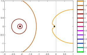
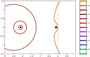
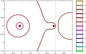
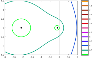
Figure 1: Boundaries of pseudospectra $\sigma_{\varepsilon}^{(1,1)}({\rm I\kern-1.25ptL}_{s},{\rm I\kern-1.25ptL})$ for four Loewner realizations of the system (14) using the interpolation points in Table 2. All four realizations correctly give $\sigma({\rm I\kern-1.25ptL}_{s},{\rm I\kern-1.25ptL})=\sigma({\bf A})$, but $\sigma_{\varepsilon}^{(1,1)}({\rm I\kern-1.25ptL}_{s},{\rm I\kern-1.25ptL})$ show how the stability of the realized eigenvalues depends on the choice of interpolation points. In this and all similar plots, the colors denote $\log_{10}(\varepsilon)$. Thus, in plot (d), there exist perturbations to ${\rm I\kern-1.25ptL}_{s}$ and ${\rm I\kern-1.25ptL}$ of norm $10^{-6.5}$ that move an eigenvalue into the right half-plane.

Table 2 records four different choices of $\{\lambda_{1},\lambda_{2},\mu_{1},\mu_{2}\}$; Figure 1 shows the corresponding pseudospectra $\sigma_{\varepsilon}^{(1,1)}({\rm I\kern-1.25ptL}_{s},{\rm I\kern-1.25ptL})$. All four Loewner realizations match the eigenvalues of ${\bf A}$ and satisfy the interpolation conditions. However, the pseudospectra show how the stability of the eigenvalues $-0.1$ and $-2.1$ differs across these four realizations. These eigenvalues become increasingly sensitive from example (a) to (d), as the interpolation points move farther from $\sigma({\bf A})$. Table 2 also shows the singular values of the Loewner matrix ${\rm I\kern-1.25ptL}$, demonstrating how the second singular value $s_{2}({\rm I\kern-1.25ptL})$ decreases as the eigenvalues become increasingly sensitive. (Taken to a greater extreme, it would eventually be difficult to determine if ${\rm I\kern-1.25ptL}$ truly is rank 2.)

Remark 5

By Remark 1 on page 1, note that if $\varepsilon<s_{\rm min}({\rm I\kern-1.25ptL})$, then $\sigma_{\varepsilon}^{(1,1)}({\rm I\kern-1.25ptL}_{s},{\rm I\kern-1.25ptL})$ will be unbounded. Thus the decreasing values of $s_{\rm min}({\rm I\kern-1.25ptL})$ in Table 2 suggests the enlarging pseudospectra seen in Figure 1. For example, in case (d) the $\varepsilon=10^{-5}$ pseudospectrum $\sigma_{\varepsilon}^{(1,1)}({\rm I\kern-1.25ptL}_{s},{\rm I\kern-1.25ptL})$ must contain the point at infinity.

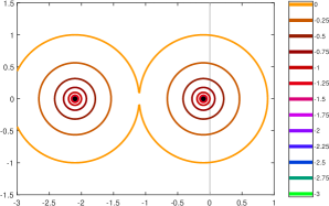
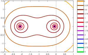
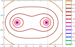
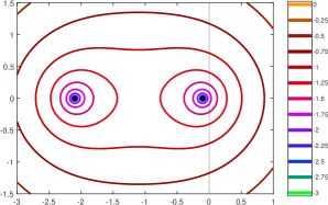
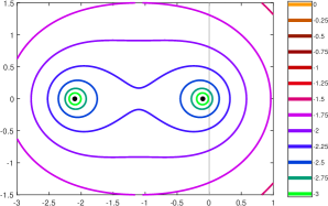
Figure 2: The pseudospectra $\sigma_{\varepsilon}({\bf A})$ (top), compared to $\sigma_{\varepsilon}({\rm I\kern-1.25ptL}^{-1}{\rm I\kern-1.25ptL}_{s})$ for four Loewner realizations of the system (14) using the interpolation points in Table 2. In all cases $\sigma({\rm I\kern-1.25ptL}^{-1}{\rm I\kern-1.25ptL}_{s})=\sigma({\bf A})$, but the pseudospectra of ${\rm I\kern-1.25ptL}^{-1}{\rm I\kern-1.25ptL}_{s}$ are all quite a bit larger than $\sigma_{\varepsilon}({\bf A})$.

Contrast these results with the standard pseudospectra of ${\bf A}$ itself, $\sigma_{\varepsilon}({\bf A})=\sigma_{\varepsilon}^{(1,0)}({\bf A},{\bf I})$ shown at the top of Figure 2. Since ${\bf A}$ is real symmetric (hence normal), $\sigma_{\varepsilon}({\bf A})$ is the union of open $\varepsilon$-balls surrounding the eigenvalues. Figure 2 compares these pseudospectra to $\sigma_{\varepsilon}({\rm I\kern-1.25ptL}^{-1}{\rm I\kern-1.25ptL}_{s})$, which give insight about the transient behavior of solutions to ${\rm I\kern-1.25ptL}\dot{\bf x}(t)={\rm I\kern-1.25ptL}_{s}{\bf x}(t)$, e.g., via the bound (11). The top plot shows $\sigma_{\varepsilon}({\bf A})$, whose rightmost extent in the complex plane is always $\varepsilon-0.1$: no transient growth is possible for this system. However, in all four of the Loewner realizations, $\sigma_{\varepsilon}({\rm I\kern-1.25ptL}^{-1}{\rm I\kern-1.25ptL}_{s})$ extends more than $\varepsilon$ into the right-half plane for $\varepsilon=10^{0}$ (orange level curve), indicating by (11) that transient growth must occur for some initial condition. Figure 3 shows this growth for all four realizations: the more remote interpolation points lead to Loewner realizations with greater transient growth.

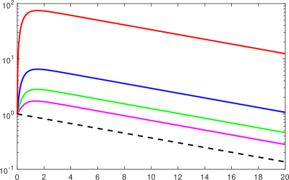
Figure 3: Evolution of the norm of the solution operator for the original system (black dashed line) and the four interpolating Loewner models. The instability revealed by the pseudospectra in Figure 2 correspond to transient growth in the Loewner systems.

6 Example 2: partitioning interpolation points and noisy data

To further investigate how the interpolation points influence eigenvalue stability, for the Loewner pencil, consider the SISO system of order 10 given by

$${\bf A}={\rm diag}(-1,-2,\ldots,-10),\quad{\bf B}=[1,1,\ldots,1]^{T},\quad{\bf C}=[1,1,\ldots,1].$$

Figure 4 shows $\sigma_{\varepsilon}^{(1,1)}({\rm I\kern-1.25ptL}_{s},{\rm I\kern-1.25ptL})$ for six configurations of the interpolation points. Plots (a) and (b) use the points $\{-10.25,-9.75,-9.25,\ldots,-1.25,-0.75\}$; in plot (a) the left and right points interlace, suggesting slower decay of the singular values of ${\rm I\kern-1.25ptL}$, as discussed in Section 2.1; in plot (b) the left and right points are separated, leading to faster decay of the singular values of ${\rm I\kern-1.25ptL}$ and considerably larger pseudospectra. (The Beckermann–Townsend bound (BT17, , Cor. 4.2) would apply to this case.) Plot (c) further separates the left and right points, giving even larger pseudospectra. In plots (d) and (f), complex interpolation points $\{-5\pm 0.5\mkern 1.0mu{\rm i},-5\pm 1.0\mkern 1.0mu{\rm i},\ldots,-5\pm 5\mkern 1.0mu{\rm i}\}$ are interleaved (while keeping conjugate pairs together) (d) and separated (f): the latter significantly enlarges the pseudospectra. Plot (f) uses the same relative arrangement that gave such nice results in plot (a) (the singular value bound (3) is the same for (a) and (e)), but their locations relative to the poles of the original system differ. The pseudospectra are now much larger, showing that a large upper bound in (3) is not alone enough to guarantee small pseudospectra. (Indeed, the pseudospectra are so large in (e) and (f) that the plots are dominated by numerical artifacts of computing $\|(z{\bf E}-{\bf A})^{-1}\|$.) Pseudospectra reveal the great influence interpolation point location and partition can have on the stability of the realized pencils.

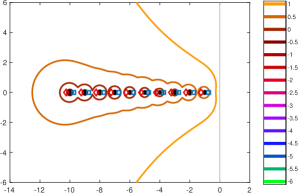
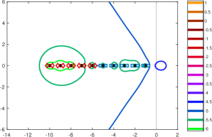
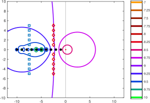
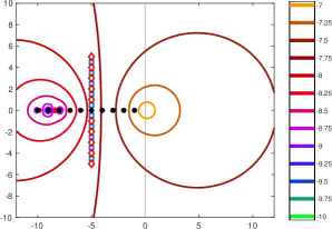
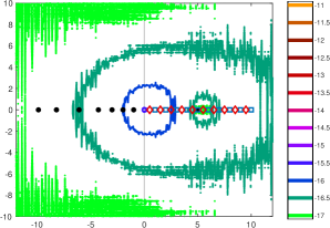
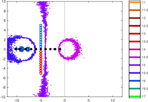
Figure 4: Pseudospectra $\sigma_{\varepsilon}^{(1,1)}({\rm I\kern-1.25ptL}_{s},{\rm I\kern-1.25ptL})$ for six Loewner realizations of a SISO system of order $n=10$ with poles $\sigma({\bf A})=\{-1,-2,\ldots,-10\}$. Black dots show computed eigenvalues of the pencil $z\mkern 1.0mu{\rm I\kern-1.25ptL}-{\rm I\kern-1.25ptL}_{s}$ (which should agree with $\sigma({\bf A})$, but a few are off axis in plot (e)); blue squares show the right interpolation points $\{\lambda_{i}\}$; red diamonds show the left points $\{\mu_{j}\}$.

Pseudospectra also give insight into the consequences of inexact measurement data. Consider the following experiment. Take the scenario in Figure 4(a), the most robust of these examples. Subject each right and left measurement $\{{\bf w}_{1},\ldots,{\bf w}_{\varrho}\}\subset\mathbbm{C}$ and $\{{\bf v}_{1},\ldots,{\bf v}_{\nu}\}\subset\mathbbm{C}$ to random complex noise of magnitude $10^{-1}$, then build the Loewner pencil $\widehat{{\rm I\kern-1.25ptL}}_{s}-z\widehat{{\rm I\kern-1.25ptL}}$ from this noisy data. How do the badly polluted measurements affect the computed eigenvalues? Figure 5 shows the results of 1,000 random trials, which can depart from the true matrices significantly:

$$3.06\leq\|\widehat{{\rm I\kern-1.25ptL}}_{s}-{\rm I\kern-1.25ptL}_{s}\|\leq 5.88,\qquad 0.49\leq\|\widehat{{\rm I\kern-1.25ptL}}-{\rm I\kern-1.25ptL}\|\leq 0.63.$$

Despite these large perturbations, the recovered eigenvalues are remarkably accurate: in $99.99\%$ of cases, the eigenvalues have absolute accuracy of at least $10^{-2}$, indeed more accurate than the measurements themselves. The pseudospectra in Figure 4(a) suggest good robustness (though the pseudospectral level curves are pessimistic by one or two orders of magnitude). Contrast this with the complex interleaved interpolation points used in Figure 4(d). Now we only perturb the data by a small amount, $5\cdot 10^{-9}$, for which the perturbed Loewner matrices (over 1,000 trials) satisfy

$$1.52\cdot 10^{-7}\leq\|\widehat{{\rm I\kern-1.25ptL}}_{s}-{\rm I\kern-1.25ptL}_{s}\|\leq 2.03\cdot 10^{-7},\qquad 2.57\cdot 10^{-8}\leq\|\widehat{{\rm I\kern-1.25ptL}}-{\rm I\kern-1.25ptL}\|\leq 3.14\cdot 10^{-8}.$$

With this mere hint of noise, the eigenvalues of the recovered system erupt: only $36.73\%$ of the eigenvalues are correct to two digits. (Curiously, $-4$ and $-5$ are always computed correctly, while $-8$, $-9$, and $-10$ are never computed correctly.) The pseudospectra indicate that the leftmost eigenvalues are more sensitive, and again hint at the effect of the perturbation (though off by roughly an order of magnitude in $\varepsilon$). Measurements of real systems (or even numerical simulations of nontrivial systems) are unlikely to produce such high accuracy; pseudospectra can reveal the virtue or folly of a given interpolation point configuration.

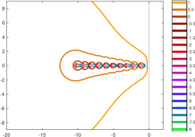
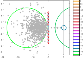
Figure 5: Eigenvalues of the perturbed Loewner pencil $\widehat{{\rm I\kern-1.25ptL}}_{s}-z\widehat{{\rm I\kern-1.25ptL}}$ (gray dots), constructed from measurements that have been perturbed by random complex noise of magnitude $10^{-1}$ (left) and $5\cdot 10^{-9}$ (right) (1,000 trials). As the pseudospectra in Figure 4(a,d) indicate, the interleaved interpolation points on the left are remarkably stable, while the similarly interleaved complex interpolation points on the right give a Loewner pencil that is incredibly sensitive to small changes in the data.

In these simple experiments, pseudospectra have been most helpful for indicating the sensitivity of eigenvalues when the left and right interpolation points are favorably partitioned (e.g., interleaved). They seem to be less precise at predicting the sensitivity to noise of poor left/right partitions of the interpolation points. Figure 6 gives an example, based on the two partitions of the same interpolation points in Figure 4(d,f). The pseudospectra suggest that the eigenvalues for plot (f) should be much more sensitive to noise than those for the interleaved points in plot (d). In fact, the configuration in plot (f) appears to be only marginally less stable to noise of size $10^{-10}$, over 10,000 trials. This is a case where one could potentially glean additional insight from structured Loewner pseudospectra.

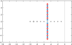
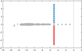
Figure 6: Eigenvalues of the perturbed Loewner pencil $\widehat{{\rm I\kern-1.25ptL}}_{s}-z\widehat{{\rm I\kern-1.25ptL}}$ (gray dots), constructed from measurements that have been perturbed by random complex noise of magnitude $10^{-10}$ (10,000 trials). As suggested by the pseudospectra plots, the interleaved interpolation points (left) are more robust to perturbations than the separated points (right), though the difference is not as acute as suggested by Figure 4(d,f). For example, in these 10,000 trials, the least stable pole ($-9$) is computed accurately (absolute error less than $.01$) in $10.97\%$ of trials on the left, and $0.29\%$ on the right.

7 Conclusion

Pseudospectra provide a tool for analyzing the stability of eigenvalues of Loewner matrix pencils. Elementary examples show how pseudospectra can inform the selection and partition of interpolation points, and bound the eigenvalues of Loewner pencils in the presence of noisy data. Using a different approach to pseudospectra, we showed that while the realized Loewner pencil matches the poles of the original system, it need not replicate transient dynamics of $\dot{\bf x}(t)={\bf A}{\bf x}(t)$; pseudospectra can reveal potential transient growth, which varies with the interpolation points.

In this initial study we have intentionally used simple examples involving small, symmetric ${\bf A}$. Realistic examples, e.g., with complex poles, nonnormal ${\bf A}$, multiple inputs and outputs, and rank-deficient Loewner matrices, will add additional complexity. Moreover, we have only used the Mayo–Antoulas interpolation theory to realize a system whose order is known; we have not addressed pseudospectra of the reduced pencils (7) in the context of data-driven model reduction.

Structured Loewner pseudospectra provide another avenue for future study. Structured matrix pencil pseudospectra have not been much investigated, especially with Loewner structure. Rump’s results for standard pseudospectra Rum06 suggest the following problem; its positive resolution would imply that the Loewner pseudospectrum $\sigma_{\varepsilon}^{(\gamma,\delta)}({\rm I\kern-1.25ptL}_{s},{\rm I\kern-1.25ptL})$ matches the structured Loewner matrix pseudospectrum.

Given any $\varepsilon,\gamma,\delta>0$, Loewner matrix ${\rm I\kern-1.25ptL}$ and associated shifted Loewner matrix ${\rm I\kern-1.25ptL}_{s}$, suppose $z\in\sigma_{\varepsilon}^{(\gamma,\delta)}({\rm I\kern-1.25ptL}_{s},{\rm I\kern-1.25ptL})$. Does there exist some Loewner matrix $\widehat{{\rm I\kern-1.25ptL}}$ and associated shifted Loewner matrix $\widehat{{\rm I\kern-1.25ptL}}_{s}$ such that

$$\|\widehat{{\rm I\kern-1.25ptL}}_{s}-{\rm I\kern-1.25ptL}_{s}\|<\epsilon\mkern 1.0mu\gamma,\qquad\|\widehat{{\rm I\kern-1.25ptL}}-{\rm I\kern-1.25ptL}\|<\epsilon\mkern 1.0mu\delta$$

and $z\in\sigma(\widehat{{\rm I\kern-1.25ptL}}_{s},\widehat{{\rm I\kern-1.25ptL}})$ ?

Appendix

We provide a MATLAB implementation that computes the inverse iteration vectors ${\bf u}$ in (12) in only ${\cal O}(n^{2})$ operations by exploiting the Cauchy-like rank displacement structure of the Loewner pencil, as shown in (13). Namely, we start from the general ${\cal O}(n^{3})$ MATLAB code from (TE05, , p. 373) and modify it to account for the Loewner structure, and hence achieve ${\cal O}(n^{2})$ efficiency. This code computes $\|(z{\rm I\kern-1.25ptL}-{\rm I\kern-1.25ptL}_{s})^{-1}\|$ for a fixed $z$. To compute pseudospectra, one applies this algorithm on a grid of $z$ values. In that case, the ${\cal O}((m+p)n^{2})$ structured LU factorization in the first line need only be computed once for all $z$ values (just as the standard algorithm computes an ${\cal O}(n^{3})$ simultaneous triangularization using the QZ algorithm once for all $z$).

  [L1,U1,piv1] = LUdispPiv(mu,lambda,[V’ L’],[R.’ -W.’]);
  L1t = L1’; U1t = U1’;
  z = 1./(z-lambda); Upz = z.*(U1\(L1\V(:,piv1)’));

  [L2,U2,piv2] = lu(eye(m)-R*Upz,’vector’); R2 = R(piv2,:);
  L2t = L2’; U2t = U2’; R2t = R2’; Upzt = Upz’;
  applyTheta = @(x) x+Upz*(U2\(L2\(R2*x)));
  applyThetaTranspose = @(x) x+R2t*(L2t\(U2t\(Upzt*x)));

  sigold = 0;
  for it = 1:maxit
      u = U1\(L1\u(piv1));
      u = conj(z).*applyThetaTranspose(applyTheta(z.*u));
      u(piv1) = L1t\(U1t\u);

      sig = 1/norm(u);
      if abs(sigold/sig-1) < 1e-2, break, end
      u = sig*u; sigold = sig;
  end
  sigmin = sqrt(sig);

The function LUdispPiv computes the LU factorization (with partial pivoting) of the Loewner matrix ${\rm I\kern-1.25ptL}$ in ${\cal O}((m+p)n^{2})$ operations. The Loewner matrix is not formed explicitly; instead, the function uses the raw interpolation data $\lambda_{i},{\bf r}_{i},{\bf w}_{i}$ and $\mu_{j},\boldsymbol{\ell}_{j},{\bf v}_{j}$. The implementation details for LUdispPiv can be found in (GV12, , sect. 12.1). The LU factorization of ${\bf I}-{\bf R}{\bf V}^{*}(z)\in\mathbbm{C}^{m\times m}$ is given by L2 and U2, while the first three lines of the loop represent the computation of ${\rm I\kern-1.25ptL}^{-*}\boldsymbol{\Theta}(z)^{*}\boldsymbol{\Theta}(z){\rm I\kern-1.25ptL}^{-1}{\bf u}$, as defined in (13). Note the careful grouping of terms and the use of elementwise multiplication .* to keep the total operation count at ${\cal O}(n^{2})$.

References

• (1) A. C. Antoulas, S. Lefteriu, and A. C. Ionita, A tutorial introduction to the Loewner framework for model reduction, in Model Reduction and Approximation: Theory and Algorithms, P. Benner, A. Cohen, M. Ohlberger, and K. Willcox, eds., SIAM, Philadelphia, 2017, pp. 335–376.
• (2) A. C. Antoulas, D. C. Sorensen, and Y. Zhou, On the decay rate of Hankel singular values and related issues, Systems Control Lett., 46 (2002), pp. 323–342.
• (3) B. Beckermann and A. Townsend, On the singular values of matrices with displacement structure, SIAM J. Matrix Anal. Appl., 38 (2017), pp. 1227–1248.
• (4) F. Chaitin-Chatelin and V. Frayssé, Lectures on Finite Precision Computations, SIAM, Philadelphia, 1996.
• (5) M. Embree, Pseudospectra, in Handbook of Linear Algebra, L. Hogben, ed., CRC/Taylor & Francis, Boca Raton, FL, second ed., 2014, ch. 23.
• (6) M. Embree and B. Keeler, Pseudospectra of matrix pencils for transient analysis of differential–algebraic equations, SIAM J. Matrix Anal. Appl., 38 (2017), pp. 1028–1054.
• (7) V. Frayssé, M. Gueury, F. Nicoud, and V. Toumazou, Spectral portraits for matrix pencils, Tech. Rep. TR/PA/96/19, CERFACS, August 1996.
• (8) I. Gohberg, T. Kailath, and V. Olshevsky, Fast Gaussian elimination with partial pivoting for matrices with displacement structure, Math. Comp., 64 (1995), pp. 1557–1576.
• (9) G. H. Golub and C. F. Van Loan, Matrix Computations, Johns Hopkins University Press, Baltimore, fourth ed., 2012.
• (10) N. J. Higham and F. Tisseur, More on pseudospectra for polynomial eigenvalue problems and applications in control theory, Linear Algebra Appl., 351–352 (2002), pp. 435–453.
• (11) D. Hinrichsen and A. J. Pritchard, Real and complex stability radii: a survey, in Control of Uncertain Systems, D. Hinrichsen and B. Mårtensson, eds., Birkhäuser, Boston, 1990.
• (12) R. A. Horn and C. R. Johnson, Matrix Analysis, Cambridge University Press, Cambridge, second ed., 2013.
• (13) P.-F. Lavallée, Nouvelles Approches de Calcul du $\varepsilon$-Spectre de Matrices et de Faisceaux de Matrices, PhD thesis, Université de Rennes 1, 1997.
• (14) A. J. Mayo and A. C. Antoulas, A framework for the solution of the generalized realization problem, Linear Algebra Appl., 425 (2007), pp. 634–662.
• (15) M. L. Overton, Numerical Computing with IEEE Floating Point Arithmetic, SIAM, Philadelphia, 2001.
• (16) T. Penzl, A cyclic low-rank Smith method for large sparse Lyapunov equations, SIAM J. Sci. Comput., 21 (2000), pp. 1401–1418.
• (17)  , Eigenvalue decay bounds for solutions of Lyapunov equations: the symmetric case, Systems Control Lett., 40 (2000), pp. 139–144.
• (18) K. S. Riedel, Generalized epsilon-pseudospectra, SIAM J. Numer. Anal., 31 (1994), pp. 1219–1225.
• (19) A. Ruhe, The rational Krylov algorithm for large nonsymmetric eigenvalues — mapping the resolvent norms (pseudospectrum). Unpublished manuscript, March 1995.
• (20) S. M. Rump, Eigenvalues, pseudospectrum and structured perturbations, Linear Algebra Appl., 413 (2006), pp. 567–593.
• (21) J. Sabino, Solution of Large-Scale Lyapunov Equations via the Block Modified Smith Method, PhD thesis, Rice University, June 2006.
• (22) F. Tisseur and N. J. Higham, Structured pseudospectra for polynomial eigenvalue problems, with applications, SIAM J. Matrix Anal. Appl., 23 (2001), pp. 187–208.
• (23) L. N. Trefethen, Computation of pseudospectra, Acta Inf., 8 (1999), pp. 247–295.
• (24) L. N. Trefethen and M. Embree, Spectra and Pseudospectra: The Behavior of Nonnormal Matrices and Operators, Princeton University Press, Princeton, NJ, 2005.
• (25) L. N. Trefethen, A. E. Trefethen, S. C. Reddy, and T. A. Driscoll, Hydrodynamic stability without eigenvalues, Science, 261 (1993), pp. 578–584.
• (26) T. G. Wright, Algorithms and Software for Pseudospectra, 2002. D.Phil. thesis, Oxford University.