Dynamical robustness of discrete conservative systems:
Harper and generalized standard maps

Abstract

In recent years, statistical characterization of the discrete conservative dynamical systems (more precisely, paradigmatic examples of area-preserving maps such as the standard and the web maps) has been analyzed extensively and shown that, for larger parameter values for which the Lyapunov exponents are largely positive over the entire phase space, the probability distribution is a Gaussian, consistent with Boltzmann-Gibbs (BG) statistics. On the other hand, for smaller parameter values for which the Lyapunov exponents are virtually zero over the entire phase space, we verify this distribution appears to approach a $q$-Gaussian (with $q=1.935\pm 0.005$), consistent with $q$-statistics. Interestingly, if the parameter values are in between these two extremes, then the probability distributions happen to exhibit a linear combination of these two behaviours. Here, we numerically show that the Harper map is also in the same universality class of the maps discussed so far. This constitutes one more evidence on the robustness of this behavior whenever the phase space consists of stable orbits. Then, we propose a generalization of the standard map for which the phase space includes many sticky regions, changing the previously observed simple linear combination behavior to a more complex combination.

I Introduction

The dynamics of the ergodic or mixing systems can be explained via notions of the Boltzmann-Gibbs (BG) statistical mechanics. For these systems, exponential and Gaussian distributions are appropriate forms to describe the limit probability behavior of relevant variables of the system under consideration. Since these distributions maximize the BG entropy, the reason behind the occurrence of such distributions can be explained by the Central Limit Theorem (CLT). On the other hand, due to the ergodicity breakdown and strong correlations among the random variables observed for some systems for some intervals of system parameters, BG statistical mechanical approaches fail to describe the dynamics of those cases and the CLT is not valid anymore. It has been shown in recent years that a generalization of the CLT is possible and the limit probability distributions seem to converge to a $q$-Gaussian distribution Umarov1 ; Umarov2 ; Nelson ; Vignat ; Umarov3 ; Hahn for a class of systems with certain correlations. Like the role of the Gaussians in the BG statistics, $q$-Gaussian distributions maximize the nonadditive entropy ($S_{q}=k(1-\sum_{i}p_{i}^{q})/(q-1)$) and constitute the basis of nonextensive statistical mechanics Tsallis ; Tsallis2010 . The nonextensive statistical mechanical framework provides a more general picture by recovering the BG statistical framework as a special case ($q\rightarrow 1$) and this generalization seems to be the appropriate tool for explaining the statistical mechanical behavior of a wide range of systems where BG statistics is known to fail.

In recent years, domains of validity of these two statistical mechanical frameworks have been shown by utilizing the rich phase space behaviors exhibited in area-preserving maps Tirnakli, (2016); Ruiz, (2017); Ruiz2017b (namely, the standard map and the web map). As the amount of nonintegrability increases with the increment of the map parameter for these Hamiltonian systems, chaotic and regular behavior regions may coexist in the phase spaces of these maps for specific parameter values. In the chaotic regions, the system is ergodic and iterates of the chaotic trajectories display uncorrelated behavior while wandering throughout the allowed region in the phase space. In this case, limit probability distribution of sums of iterates of the map converges to a Gaussian consistently with assertions of the BG statistical mechanical framework. On the other hand, iterates of trajectories starting from initial conditions located inside the nonergodic stability islands exhibit strongly correlated behavior. For these initial conditions, it has been shown for the standard map Tirnakli, (2016); Ruiz, (2017) and the web map Ruiz2017b that the limit probability distribution converges to a $q$-Gaussian with a specific $q=1.935\pm 0.005$ value. When the entire system is modeled by using initial conditions coming from both chaotic sea and stability islands for some specific parameter values, the limit probability distribution is obtained as a linear combination of a Gaussian and a $q$-Gaussian with $q=1.935\pm 0.005$; the $q$-Gaussian distribution maintains its existence together with Gaussian even for large number of iteration steps. This limit distribution seems very robust from the statistical mechanical point of view since the same distribution appears for the initial conditions selected from stability islands of different maps. Any novel understanding of such systems would no doubt be important if we consider the role of the area-preserving maps in physics and in the development of the chaos theory Hilborn . Many physical systems such as magnetic traps Chirikov1987 , electron magnetotransport in classical and quantum wells Shepelyansky , particle accelerators Izraelev can be modeled by using the standard map as a first approximation. In addition, linear combination of the standard map and the web map can be used for modeling many physical systems Zaslavsky, (1991). As the area-preserving maps have such importance in different branches, whether the common limit probability behavior observed for initial conditions of the stability islands of the standard map and the web map is a universal behavior for all area-preserving maps would be a very intriguing research question that deserves to be investigated. In this study, to test the robustness of the $q$-Gaussian distribution with $q=1.935\pm 0.005$, we analyze the limit behavior of the sums of the iterates of the Harper map harper , which models transport phenomena in deterministic chaotic Hamiltonian systems. In addition to the Harper map, we also define a new generalized form for the standard map, namely $z$-generalized standard map, to create independent and unique area-preserving maps exhibiting different phase space dynamics.

In order to statistically characterize these area-preserving maps we choose various map parameter values for each system where the phase spaces display different behavior. As the phase spaces of these scenarios provide rich observations by exhibiting chaotic and regular behaviors at the same time for specific parameter values, we numerically investigate the limit probability distribution of the entire system and visualize how the limit distributions vary according to the map parameter value. For each case we obtain phase space portraits given in this paper by iterating $40$-$50$ randomly chosen initial conditions $T=5\times 10^{3}$ times. In order to quantify the trajectory behaviors seen in the phase portraits we calculate the largest Lyapunov exponent, LLE ($\lambda$), by using Benettin algorithm Benettin86 for each initial condition randomly chosen from the entire phase space. Lyapunov exponents are calculated over $T=5\times 10^{5}$ time steps using $M=5\times 10^{5}$ initial conditions and Lyapunov spectra of scenarios are portrayed via color maps in order to reveal the regions with different behavior. Since the chaotic regions and the stability islands exhibit largely positive and nearly zero LLE values respectively, this separation of the phase space regions allows us to distinguish the portions of the phase space where the system appears to be ergodic and nonergodic Tirnakli, (2016). Chaotic trajectories presenting largely positive LLE values diverge exponentially in the allowed region of the phase space and these trajectories spread into this region with apparently random behavior. For the strongly chaotic regions, system exhibits mixing property and ergodic behavior. On the other hand, trajectories located inside the stability islands, which can be periodic or quasi-periodic, present nearly zero LLE values ($\lambda\approx 0$) and the system is nonergodic in these regions. Although argument about the ergodicity of the chaotic trajectories is verified for numerous dissipative Afsar2013 ; Cetin2015 and conservative Tirnakli, (2016); Ruiz, (2017); Ruiz2017b systems, we come across with a contrary situation for sticky chaotic regions that may arise in several $z$-generalized standard map systems by exhibiting nonergodic behavior for finite observation times. This unexpected behavior will be further discussed later on, when analyzing the $z$-generalized standard map.

Since the ergodic and nonergodic portions of the phase space require different statistical mechanical approaches, we can investigate the limit probability distributions of the variables of the systems to determine the domains of validity of the BG and of the nonextensive statistical mechanics. In the spirit of the Central Limit Theorem, for the limit probability distribution characterization, we define the variable

$$y=\frac{1}{\sqrt{T}}\sum_{i=1}^{T}\left(x_{i}-\langle\,x\,\rangle\right)$$ (1)

where $x$ is the variable of the map, $\langle\,\cdots\rangle$ denotes averaging over a large number of iterations $T$ and a large number of randomly chosen initial conditions $M$, i.e., $\langle x\rangle=\frac{1}{M}\frac{1}{T}\sum_{j=1}^{M}\sum_{i=1}^{T}x_{i}^{(j)}$. It was previously shown, for arbitrary values of the parameter $K$ of the standard map Tirnakli, (2016); Ruiz, (2017), that the probability distribution of these sums (Eq. (1)) can be modeled as

$$P_{q}(y;\mu_{q},\sigma_{q})=A_{q}\sqrt{B_{q}}\left[1-(1-q)B_{q}(y-\mu_{q})^{2}\right]^{\frac{1}{1-q}},$$ (2)

that represents the probability density for the initial conditions inside the vanishing Lyapunov region ($q\neq 1$), where $\mu_{q}$ is the $q$-mean value, $\sigma_{q}$ is the $q$-variance, $A_{q}$ is the normalization factor and $B_{q}$ is a parameter which characterizes the width of the distribution prato-tsallis-1999 :

$$A_{q}=\left\{\begin{array}[]{lc}\displaystyle\frac{\Gamma\left[\frac{5-3q}{2(1-q)}\right]}{\Gamma\left[\frac{2-q}{1-q}\right]}\sqrt{\frac{1-q}{\pi}},&q<1\\ \displaystyle\frac{1}{\sqrt{\pi}},&q=1\\ \displaystyle\frac{\Gamma\left[\frac{1}{q-1}\right]}{\Gamma\left[\frac{3-q}{2(q-1)}\right]}\sqrt{\frac{q-1}{\pi}},&1<q<3\end{array}\right.$$ (3)

$$B_{q}=[(3-q)\sigma_{q}^{2}]^{-1}.$$ (4)

The $q$-mean value and $q$-variance are defined by (see prato-tsallis-1999 for the continuous version):

$$\mu_{q}=\frac{\sum_{i=1}^{N}y_{i}[P_{q}(y_{i})]^{q}}{\sum_{i=1}^{N}[P_{q}(y_{i})]^{q}},$$ (5)

$$\sigma_{q}^{2}=\frac{\sum_{i=1}^{N}y_{i}^{2}[P_{q}(y_{i})]^{q}}{\sum_{i=1}^{N}[P_{q}(y_{i})]^{q}},$$ (6)

though we have considered these variables as fitting parameters.

The $q\to 1$ limit recovers the Gaussian distribution $P_{1}(y;\mu_{1},\sigma_{1})=\frac{1}{\sigma_{1}\sqrt{2\pi}}\exp\left[-\frac{1}{2}\left(\frac{y-\mu_{1}}{\sigma_{1}}\right)^{2}\right]$. In the analyses of the limit probability distributions of such maps with various values for the map parameter, we randomly choose a large number of initial conditions, larger than $3\times 10^{7}$, from the entire phase space, and numerically calculate the limit distribution of Eq. 1 using $T=2^{22}$ iteration steps in order to obtain a good statistical description of the systems. These values are determined in accordance with the recent works Tirnakli, (2016); Ruiz, (2017) where they have been shown to be optimal by considering required computational times and convergence of the obtained probability distributions.

This paper is organized as follows: Firstly, the Harper map and the $z$-generalized standard map will be introduced in Sections II and III; then the results of the numerical calculations are discussed in Section IV. Finally we conclude in the last section.

II Harper Map

In order to investigate transport phenomena in deterministic chaotic Hamiltonian dynamics, a two-dimensional area-preserving map has been proposed in harper using a time-dependent Hamiltonian of the form

$$\begin{array}[]{l}H(x,p,t)=-V_{2}\cos(2\pi p)-V_{1}\cos(2\pi x)\tau\sum_{n=-\infty}^{\infty}\delta(t-n\tau).\end{array}$$ (7)

This is called kicked Harper model and has several applications in physics harperApp1 ; harperApp2 ; harperApp3 . If one integrate Eq.(7) over one period $\tau$ of the kicking potential, the kicked Harper map can be obtained easily as follows:

$$\begin{array}[]{l}p_{i+1}=p_{i}-\gamma_{1}\sin(2\pi x_{i})\\ x_{i+1}=x_{i}+\gamma_{2}\sin(2\pi p_{i+1})\end{array}$$ (8)

where $p$ and $x$ are taken as modulo $1$ and $\gamma_{j}=2\pi V_{j}\tau$. In the present paper, we will only consider the special case $\gamma_{1}=\gamma_{2}\equiv\gamma$.

III Generalized Standard Map

The Hamiltonian of the standard map is given by Zaslavsky2007

$$H=\frac{1}{2}p^{2}-K\cos(x)\sum_{n=-\infty}^{\infty}\delta\left(\frac{t}{T}-n\right)\\$$ (9)

where $p$ and $x$ are the momentum and position of a particle respectively and the periodic sequence of $\delta$-pulses has the period $T=2\pi/\nu$. The equations of motion derived from this Hamiltonian enables us to write down the momentum and position variables at the $n$-th and ($n+1$)-th kicks, from where the original standard map is obtained Chirikov1979 . One possible way of generalizing the original standard map is to modify the kicked term as $(K/z)\cos(zx)$, which results in defining the $z$-generalized standard map as follows:

$$\begin{array}[]{l}p_{i+1}=p_{i}-K\sin(zx_{i})\\ x_{i+1}=x_{i}+p_{i+1}\end{array}$$ (10)

where $p$ and $x$ are taken as modulo $2\pi$, $K$ is the map parameter which controls the amount of nonintegrability of the system and $z$ is an integer; $z=1$ recovers the usual standard map. With different $z$ values we define unique systems exhibiting specific phase-space dynamics. In this paper we investigate the phase-space behaviors and the limit distributions for various $z$ values with $K=0.2$ and $K=0.6$ parameters by using the numerical calculations introduced in the Introduction section. In order to present a clear evolution for the phase portraits and the limit distributions according to the $z$ generalization term, we analyze $z=3$, $z=5$, $z=40$ generalized systems for $K=0.2$, and $z=3$, $z=4$, $z=15$ systems for $K=0.6$. For both parameter values we also analyze the $z=1$ system (the original standard map) in order to study how the $z$-generalization modifies the dynamical and statistical behavior of the system.

IV Results

As discussed in harper , in the Harper map phase-space plots, a separatrix defined by $H_{0}(p,x)=0$ appears and forms a square symmetry. When $\gamma>0$, this separatrix is destroyed and becomes a mesh of finite thickness inside which the dynamics is chaotic. This region grows as $\gamma$ increases, making the region of the regular motion to shrink. This behavior is evident from the first column of Fig. 1 for some representative $\gamma$ values. Then, in the second column, one can see the Lyapunov diagram for the same values of $\gamma$. The genesis and increasing domination of the chaotic sea can be clearly seen as $\gamma$ increases. Finally, the last column exhibits the corresponding probability distributions. As discussed extensively in Ruiz, (2017); Ruiz2017b , these distributions can be well approximated by a linear combination of one Gaussian and one $q$-Gaussian distributions, namely,

$$P(y)=\alpha_{q_{1}}P_{q_{1}}(y;\mu_{q_{1}},\sigma_{q_{1}})+\alpha_{q_{2}}P_{q_{2}}(y;\mu_{q_{2}},\sigma_{q_{2}})$$ (11)

where $q_{1}=1.935\pm 0.005$ and $q_{2}=1$. In Eq. 11, the contribution ratios $\alpha_{q_{1}}$ and $\alpha_{q_{2}}$ can be evaluated from the phase-space occupation ratios of initial conditions located in the stability islands and chaotic sea detected from the Lyapunov color map, respectively. Therefore, these parameters are not fitting parameters, but determined directly from the dynamics of the system. The $q$-Gaussian distribution with $q=1.935\pm 0.005$ originates from the initial conditions of the stability islands, and initial conditions from the chaotic sea contributes to the Gaussian distribution. The obtained results for the parameters are given in Table. 1. These results clearly show that the Harper is in the same universality class of the standard map and the web map, and therefore provide one more argument pointing to the robustness of the $q$-Gaussian with $q=1.935\pm 0.005$.

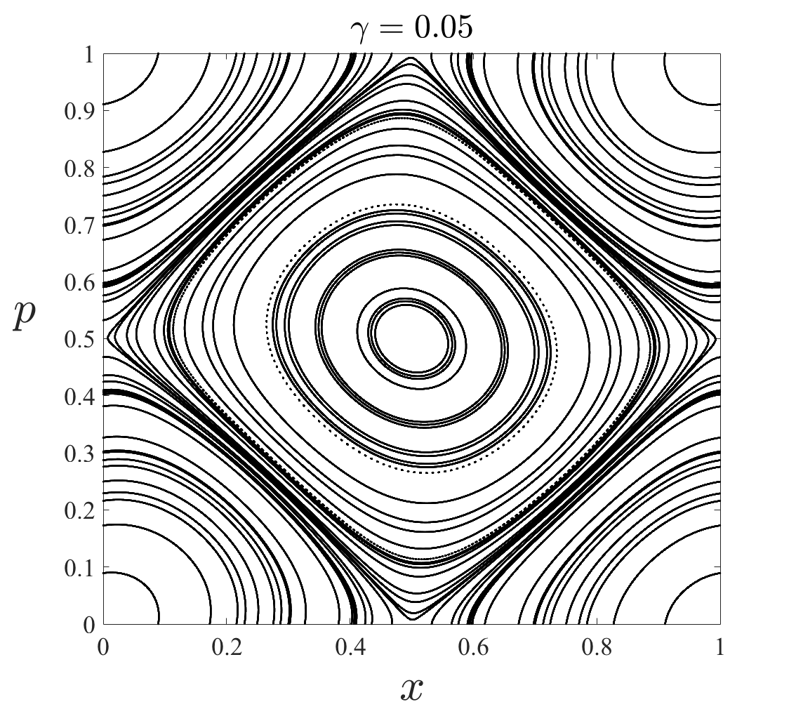
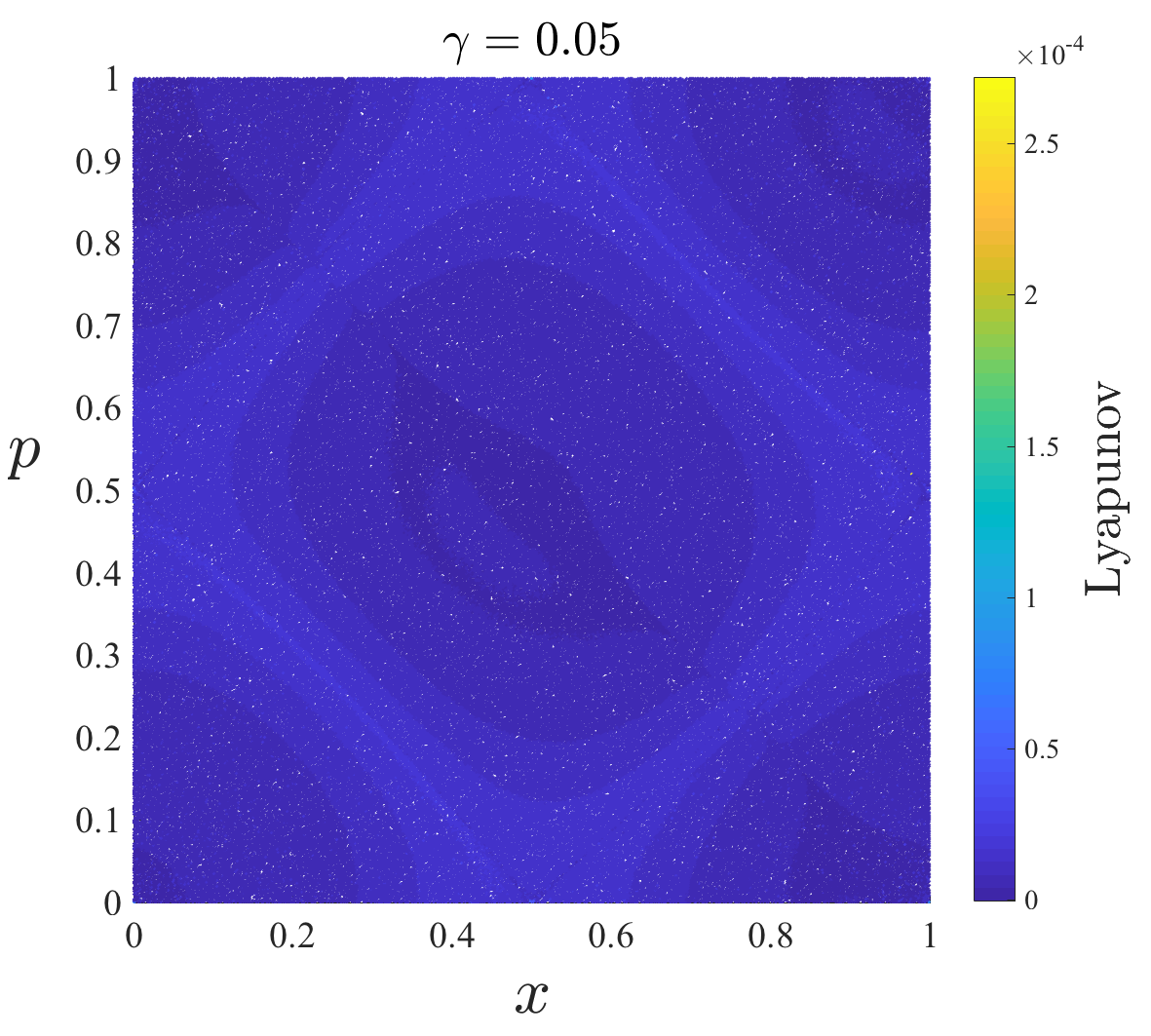
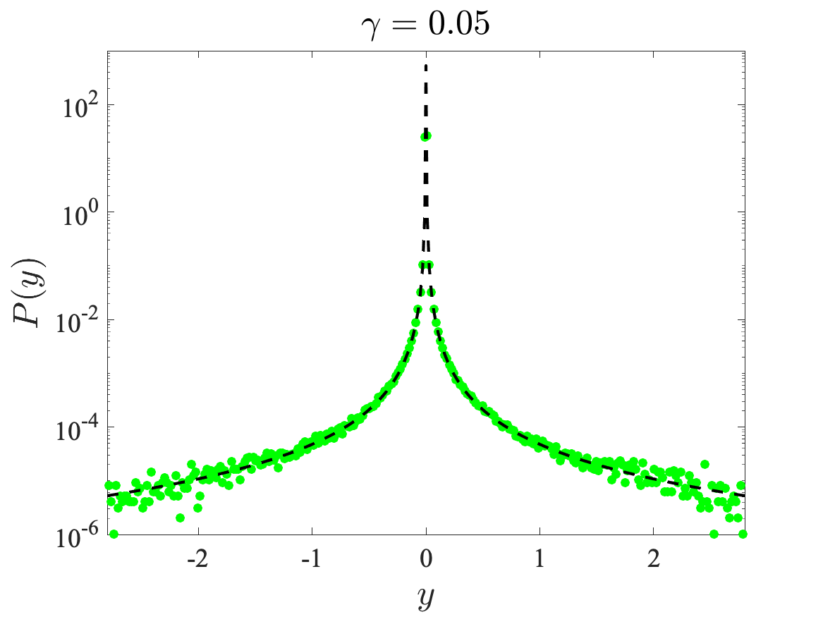
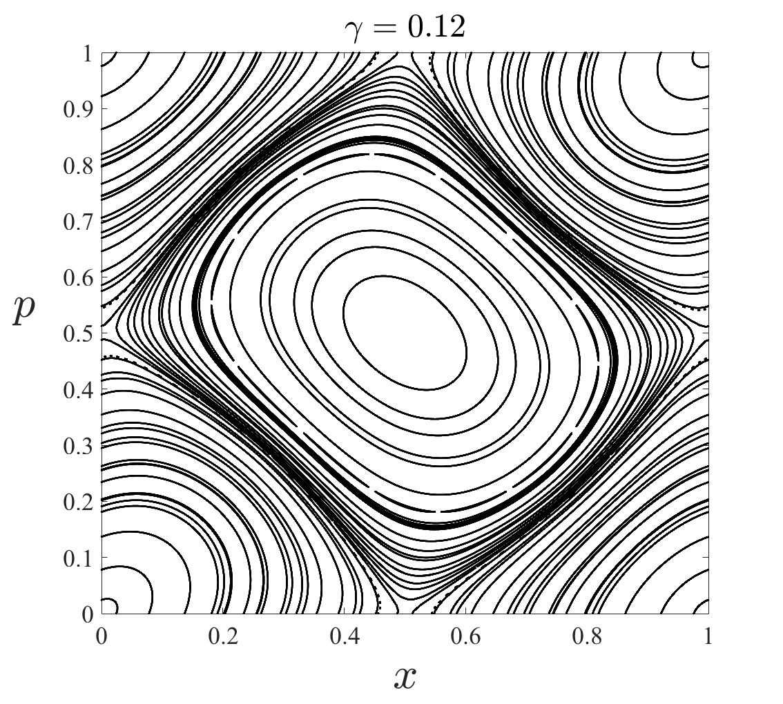
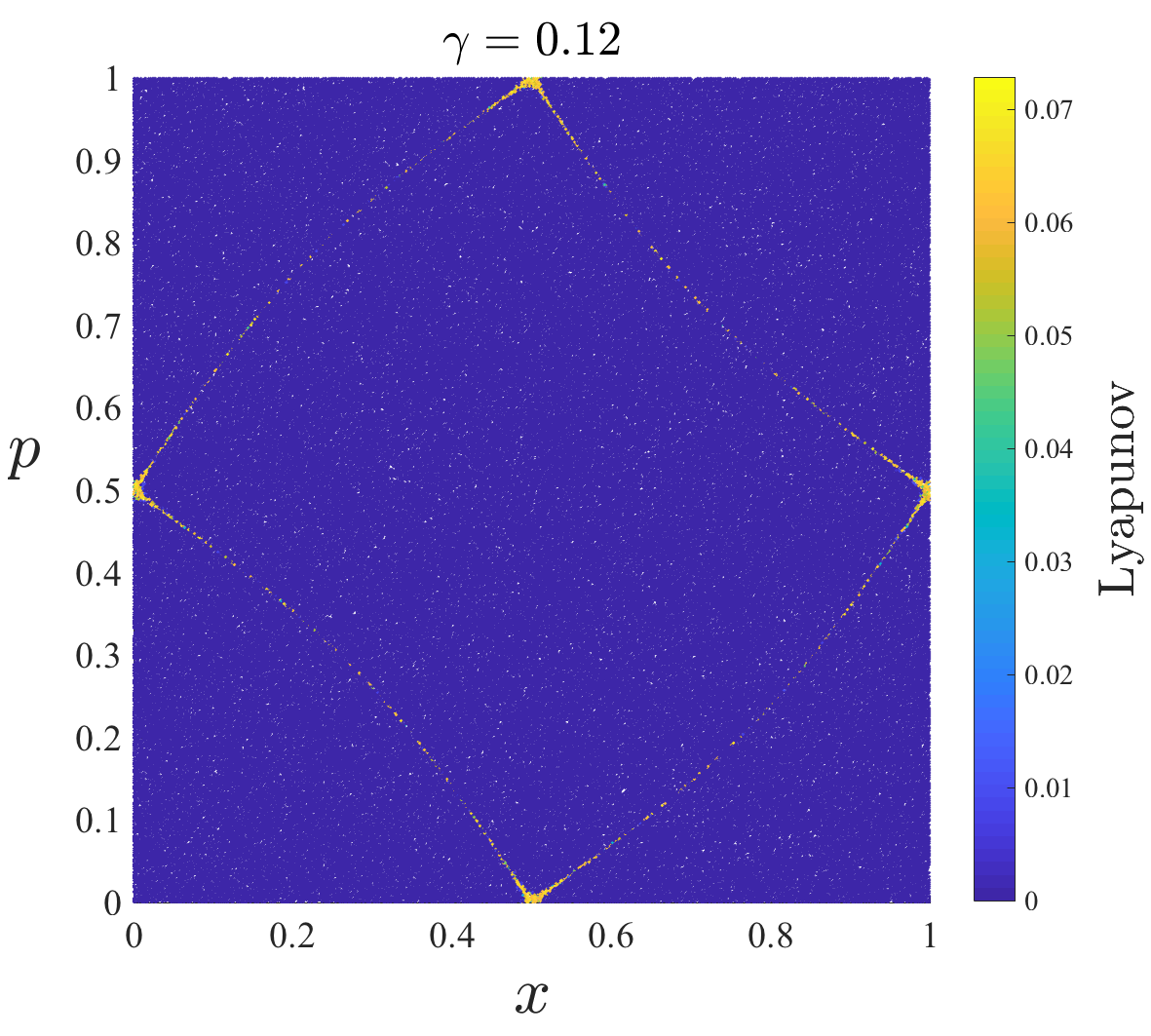
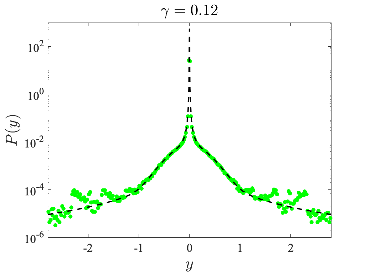
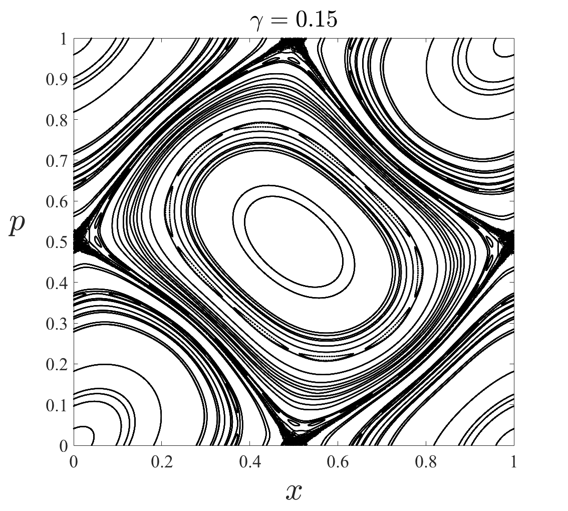
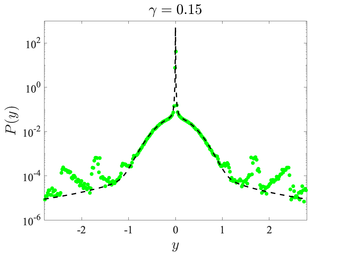
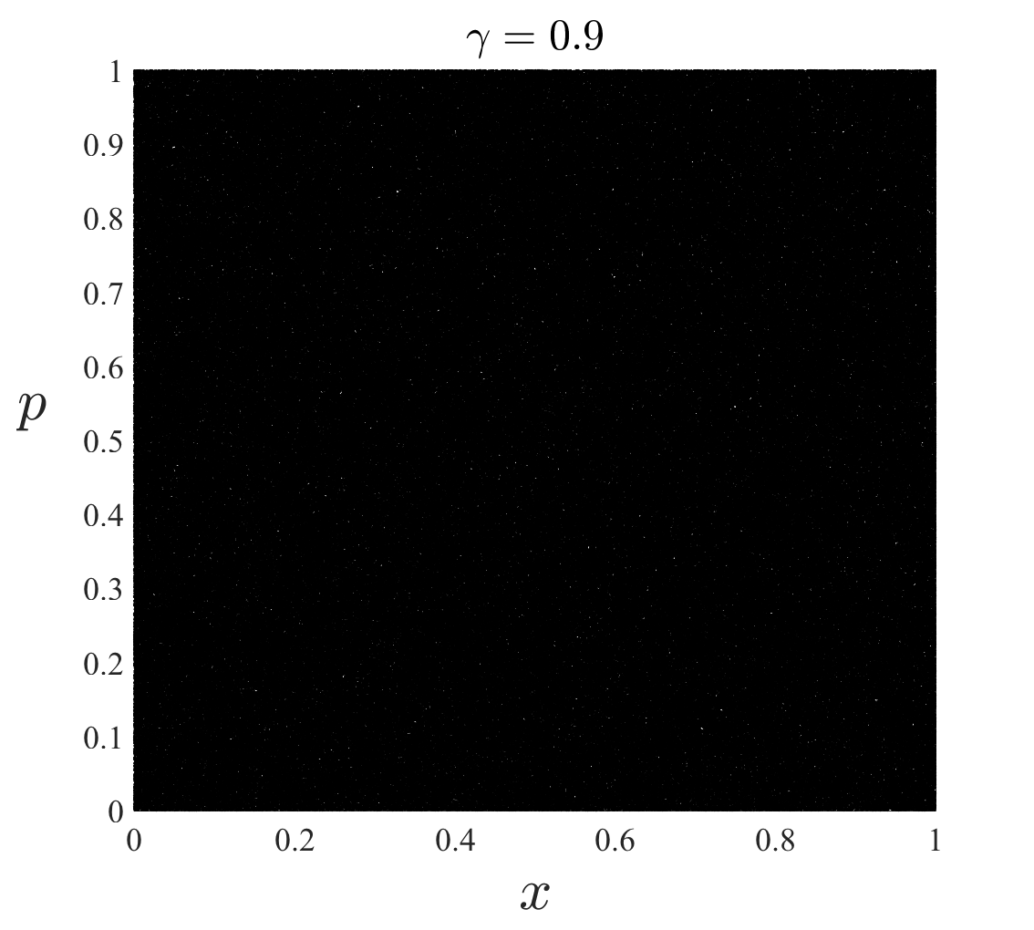
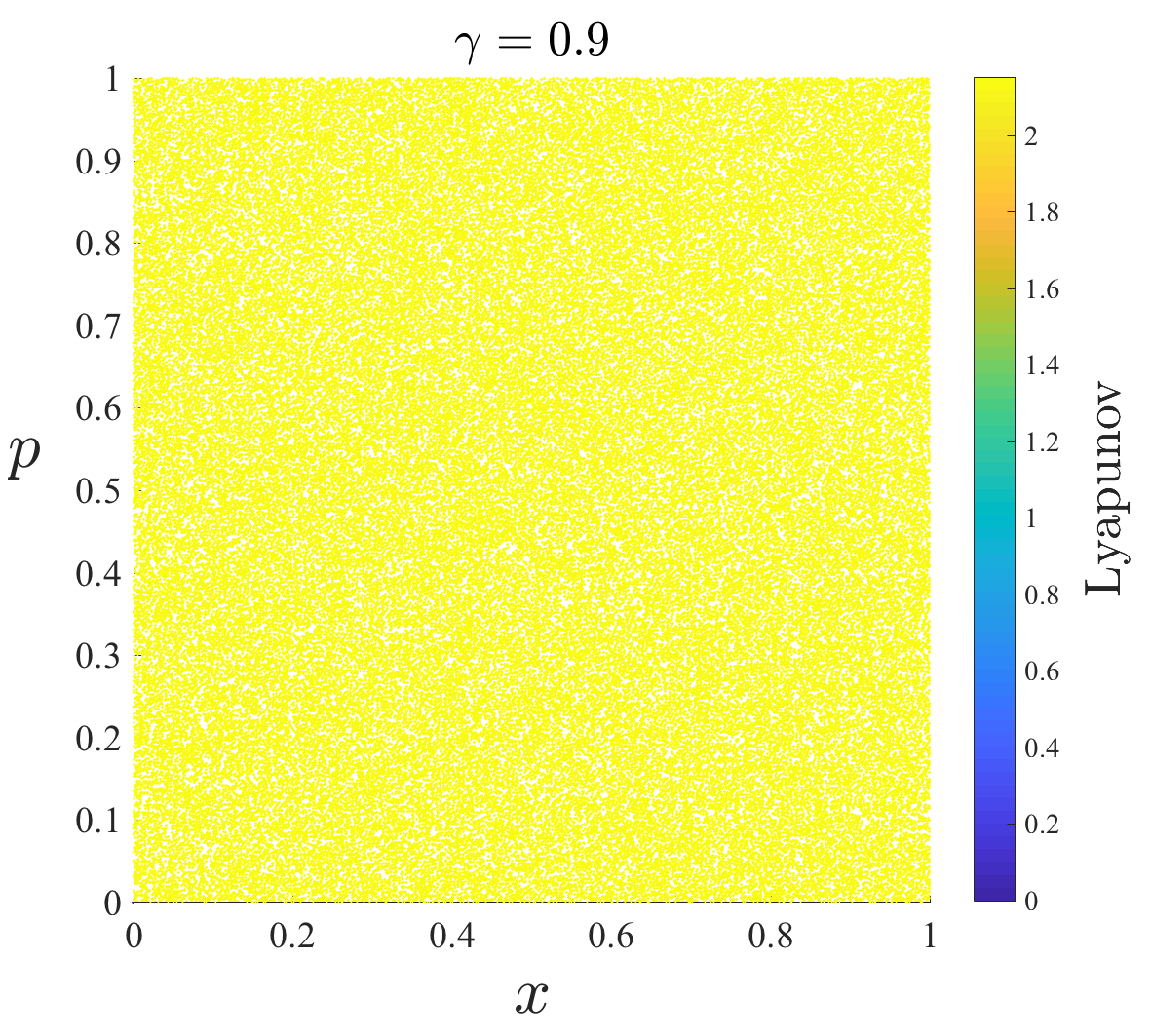
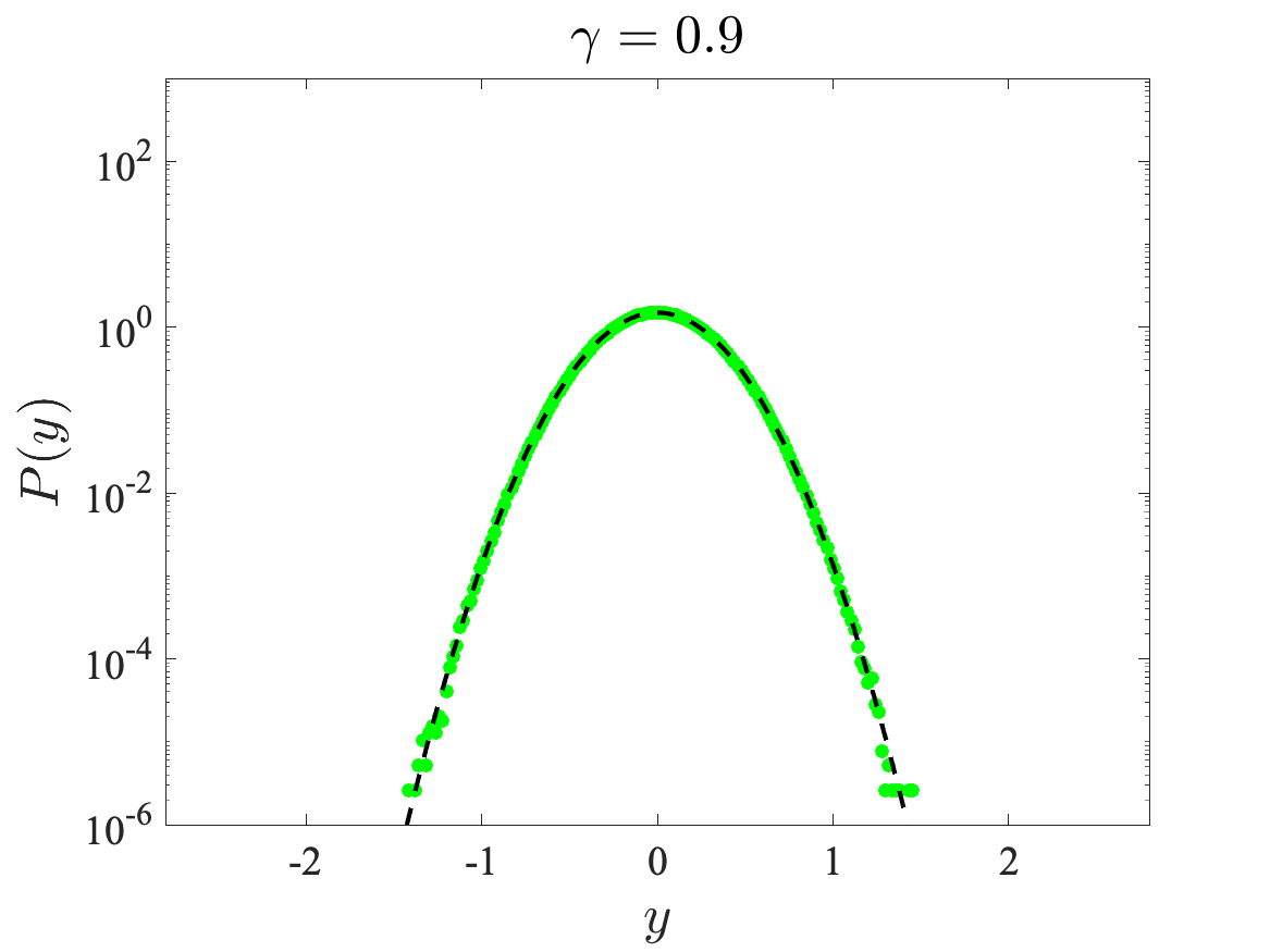
Figure 1: (Color online) Left column: Phase space portrait of the Harper map for various $\gamma$ values; 40-50 initial conditions have been used in each case. Middle column: Lyapunov diagrams for the same values of $\gamma$. The Lyapunov exponents have been calculated over 500000 time steps using 500000 initial conditions taken randomly from the entire phase space. Right column: Probability distributions obtained from the same values of $\gamma$. In all cases, the number of initial conditions is larger than $3\times 10^{7}$ in order to achieve good statistics.

Table 1: Obtained results for the Harper map for four representative values of $\gamma$.

	$\gamma=0.05$	$\gamma=0.12$	$\gamma=0.15$	$\gamma=0.9$
$q_{1}$	1.935	1.935	1.935	1.935
$q_{2}$	1	1	1	1
$\alpha_{q_{1}}$	1	0.9960	0.9713	0
$\alpha_{q_{2}}$	0	0.0040	0.0287	1
$B_{q_{1}}$	$65\times 10^{5}$	$25\times 10^{5}$	$25\times 10^{5}$	-
$B_{q_{2}}$	-	$5.3$	$5.7$	$7.0$

Now, we can concentrate on the $z$-generalized standard map. Phase-space portraits of representative cases, their corresponding Lyapunov diagrams, and the limit probability distributions are given in Fig. 2 for $K=0.2$ and in Fig. 3 for $K=0.6$. They enable to visualize how the dynamics of these systems change according to the increment of the $z$ term. Surprisingly, we noticed that these distributions cannot be modeled using Eq. 11. Instead, we verified that, for this system, the obtained distributions happen to be well approximated by a linear combination of three $q$-Gaussian distributions, namely,

$$P(y)=\alpha_{q_{1}}P_{q_{1}}(y;\mu_{q_{1}},\sigma_{q_{1}})+\alpha_{q_{2}}P_{q_{2}}(y;\mu_{q_{2}},\sigma_{q_{2}})+\alpha_{q_{3}}P_{q_{3}}(y;\mu_{q_{3}},\sigma_{q_{3}}).$$ (12)

The probability distributions given in Fig. 2 and Fig. 3 can be well approximated by this linear combination. The relevant parameter values are given in Table. 2.

Table 2: Obtained results for the $z$-generalized standard map for representative values of $z$ and $K$.

	$K=0.2$		$K=0.6$
	$z=3$	$z=5$	$z=3$	$z=4$
$q_{1}$	1.935	1.935	1.935	1.935
$q_{2}$	1.40	1.55	1.40	1.55
$q_{3}$	1	1.45	1	1
$\alpha_{q_{1}}$	0.963	0.515	0.265	0.114
$\alpha_{q_{2}}$	0.025	0.340	0.565	0.300
$\alpha_{q_{3}}$	0.012	0.145	0.170	0.586
$B_{q_{1}}$	60000	25800	25300	2000
$B_{q_{2}}$	$0.389$	$0.072$	$0.0215$	$0.0039$
$B_{q_{3}}$	$0.00015$	$0.004$	$0.0455$	$0.0025$

In Fig. 2, we see that the phase spaces of $z=1$ and $z=40$ systems are entirely occupied by nonergodic stability islands and ergodic chaotic sea, respectively. Conformably with these phase space behaviors, the probability distribution of Eq. 1 obtained for the initial conditions randomly chosen from the entire phase space is well fitted by a Gaussian when the system is ergodic-like and by a $q$-Gaussian with $q\simeq 1.935$ when the system is nonergodic-like. In Fig. 3, for $K=0.6$, the occurrence of a Gaussian as a limit distribution of the initial conditions chosen from the ergodic phase space is also verified for $z=15$ system whose phase space is occupied by the chaotic sea. For $K=0.6$ parameter value of the $z=1$ system which corresponds to the original standard map, the phase space consists of both stability islands and the chaotic sea. In accordance with recent works Tirnakli, (2016); Ruiz, (2017), the limit probability distribution of Eq. 1, given in Fig. 3, is obtained as a linear combination of a Gaussian arises from the initial conditions located in the chaotic sea and a $q$-Gaussian with $q=1.935\pm 0.005$ arises from the initial conditions located in the stability islands. By considering the regions of different behaviors that the phase space consists of, These limit distributions are of course expected due to the ergodic/nonergodic behavior of the related phase space. Here contribution ratios of each term in the linear combination are detected using the Lyapunov spectrum, and therefore they are not fitting parameters but determined directly from the dynamics of the system.

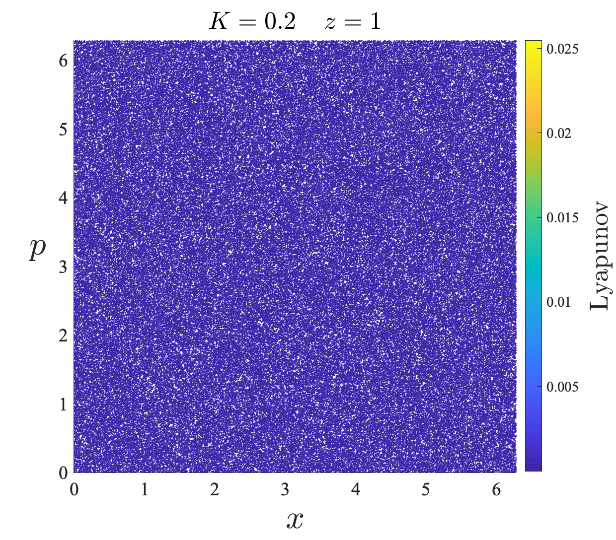
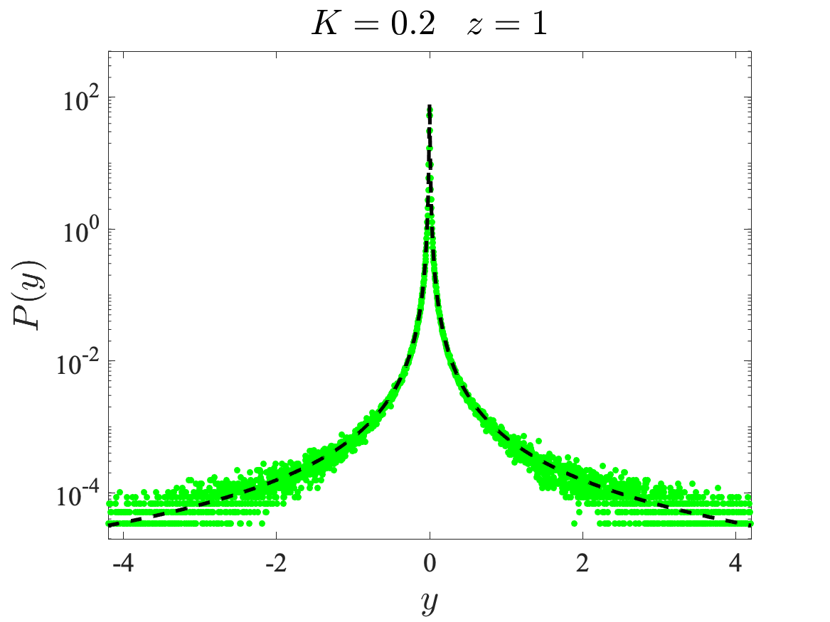
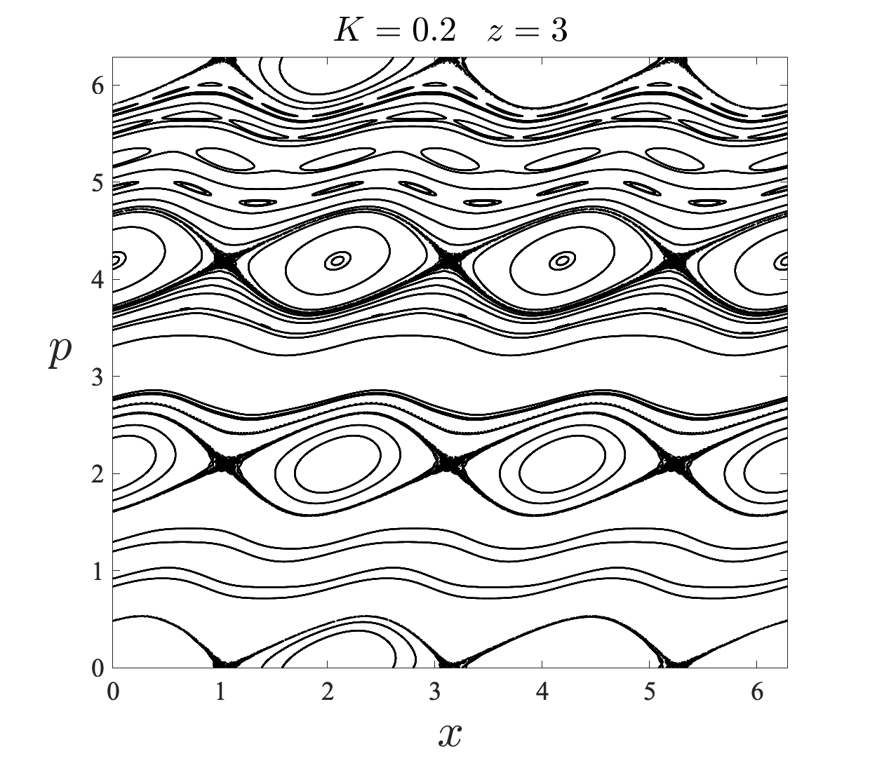
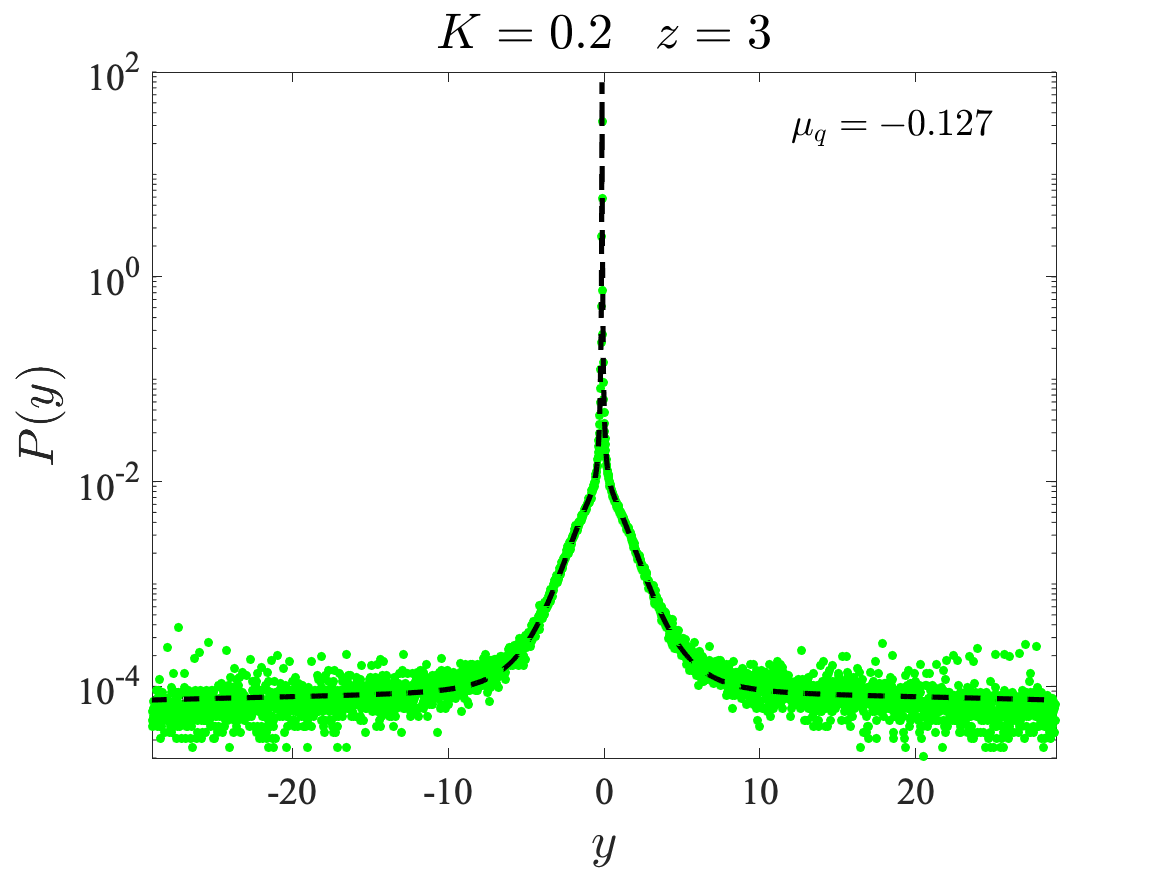
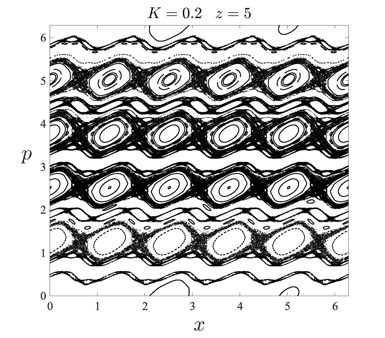
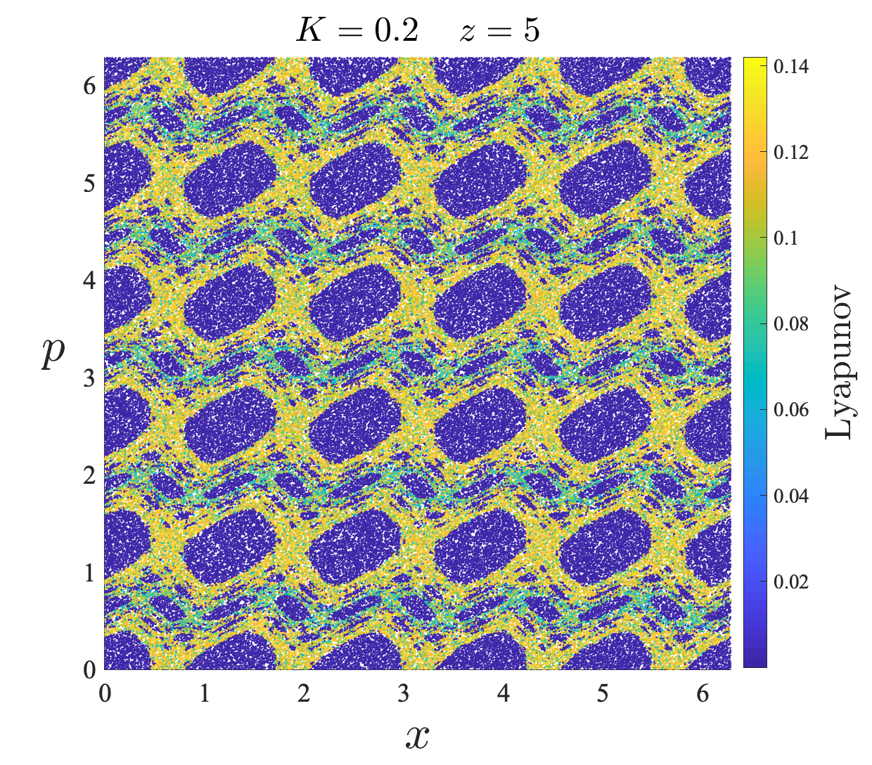
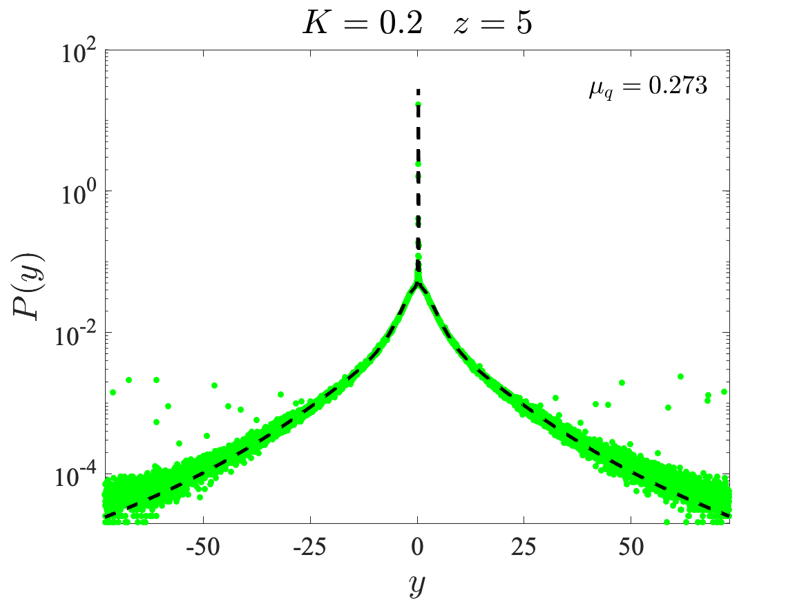
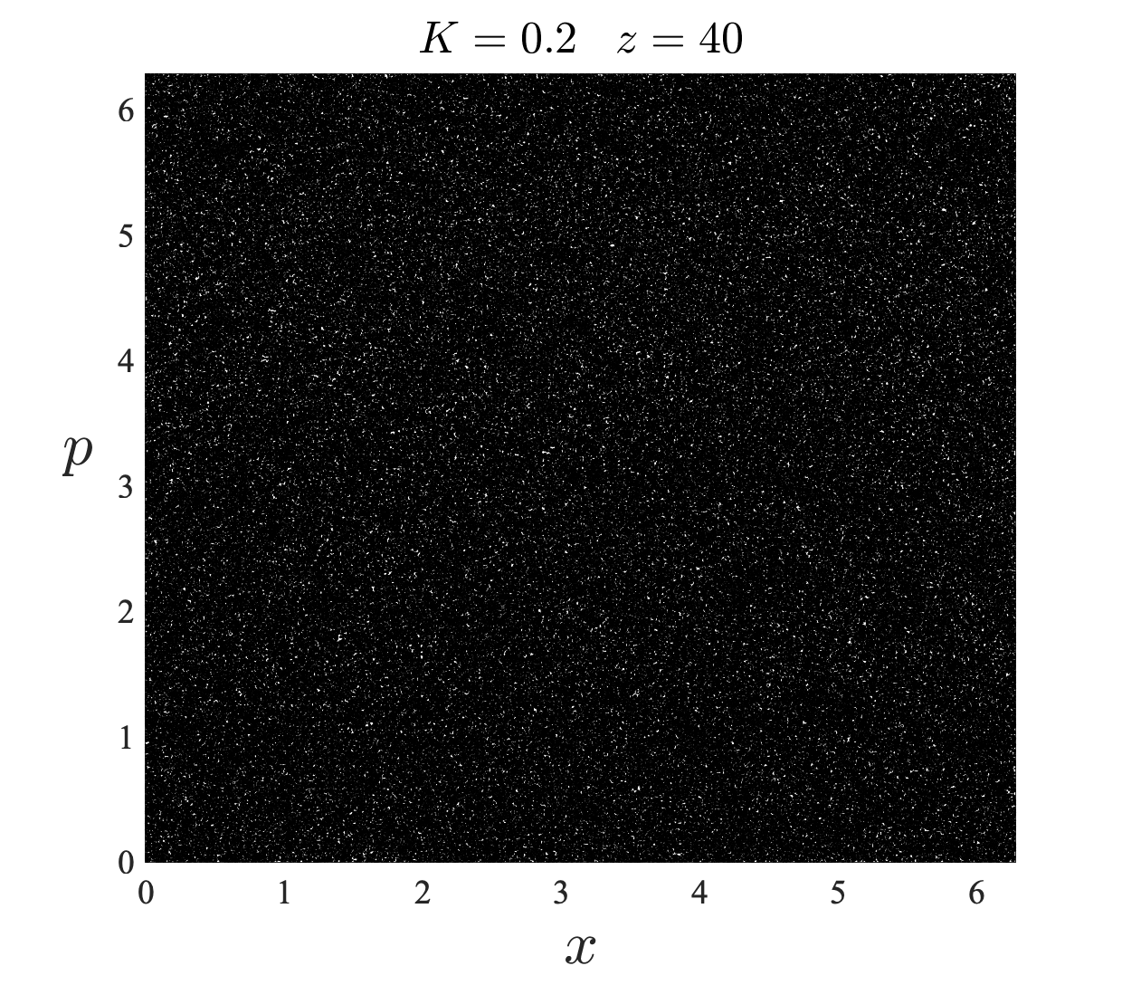
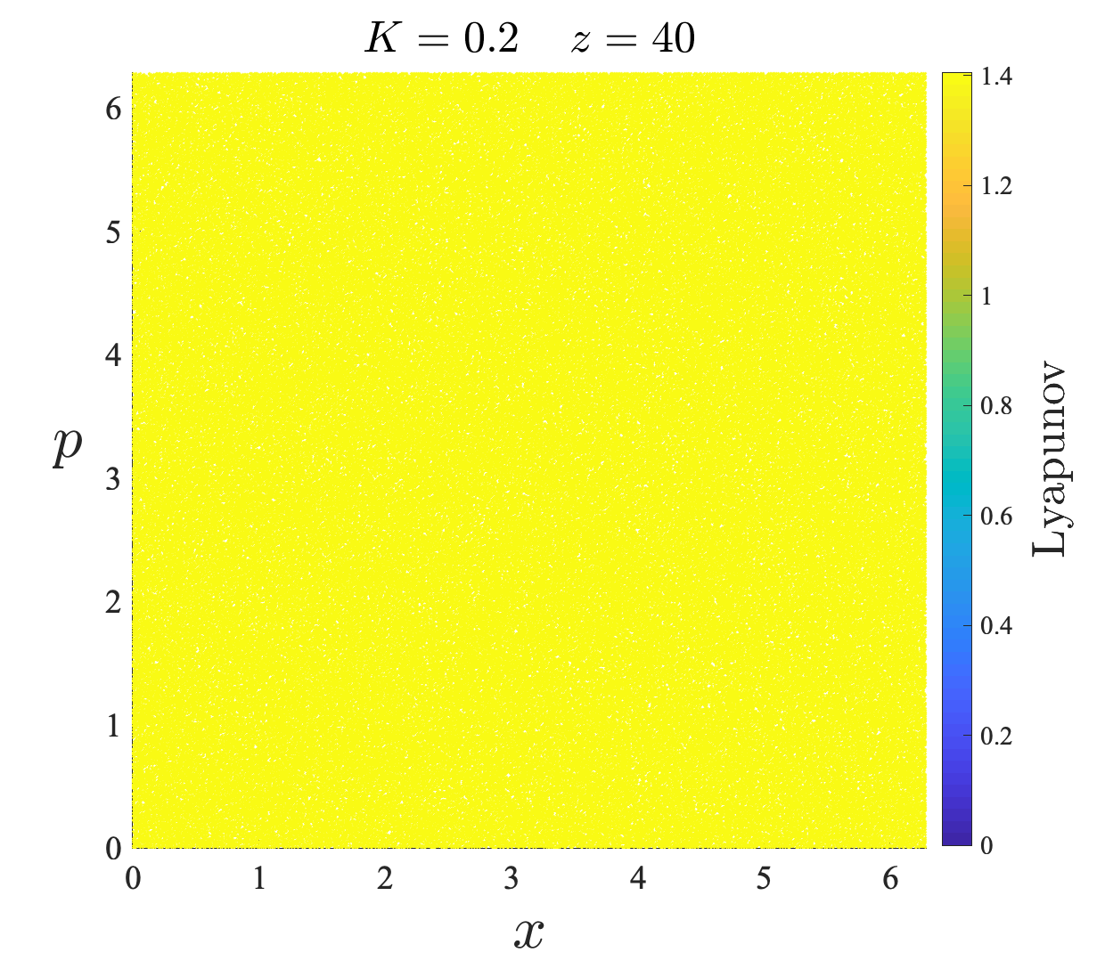
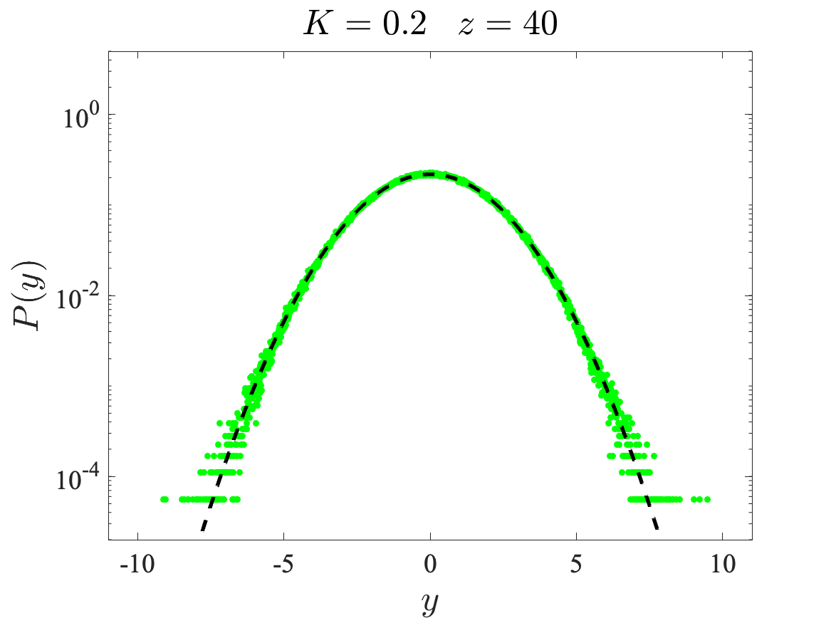
Figure 2: (Color online) Left column: Phase space portrait of the $z$-standard map for $K=0.2$ with various $z$ values; 40-50 initial conditions have been used in each case. Middle column:  Lyapunov diagrams for the same cases. The Lyapunov exponents have been calculated over 500000 time steps using 500000 initial conditions taken randomly from the entire phase space. Right column: Probability distributions obtained for the same cases. In all cases, the number of initial conditions is larger than $3\times 10^{7}$ in order to achieve good statistics.

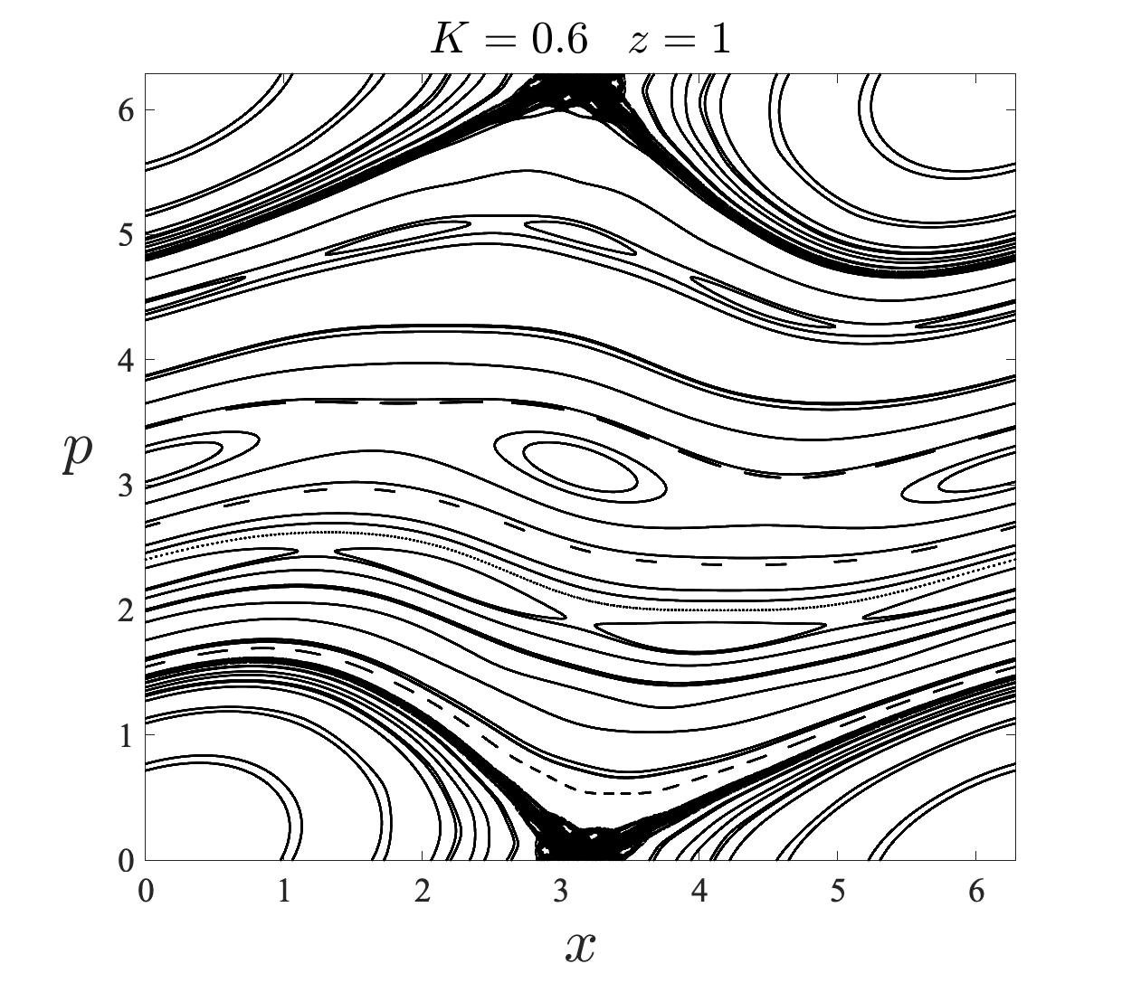
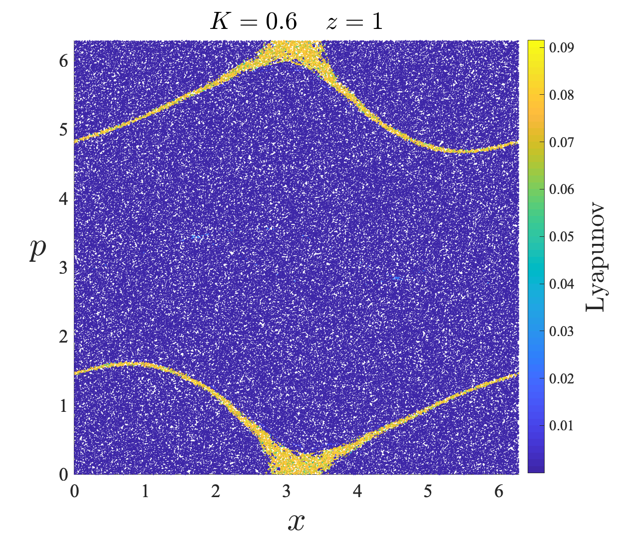
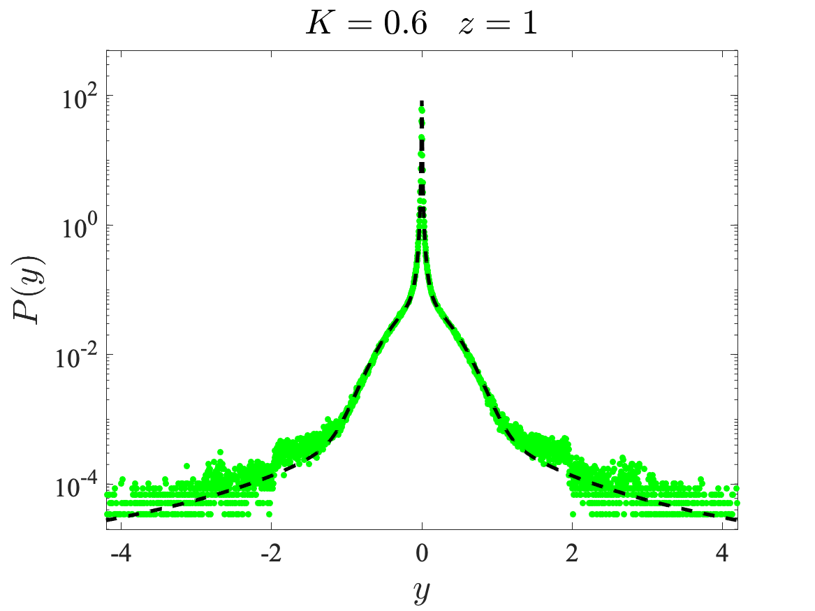
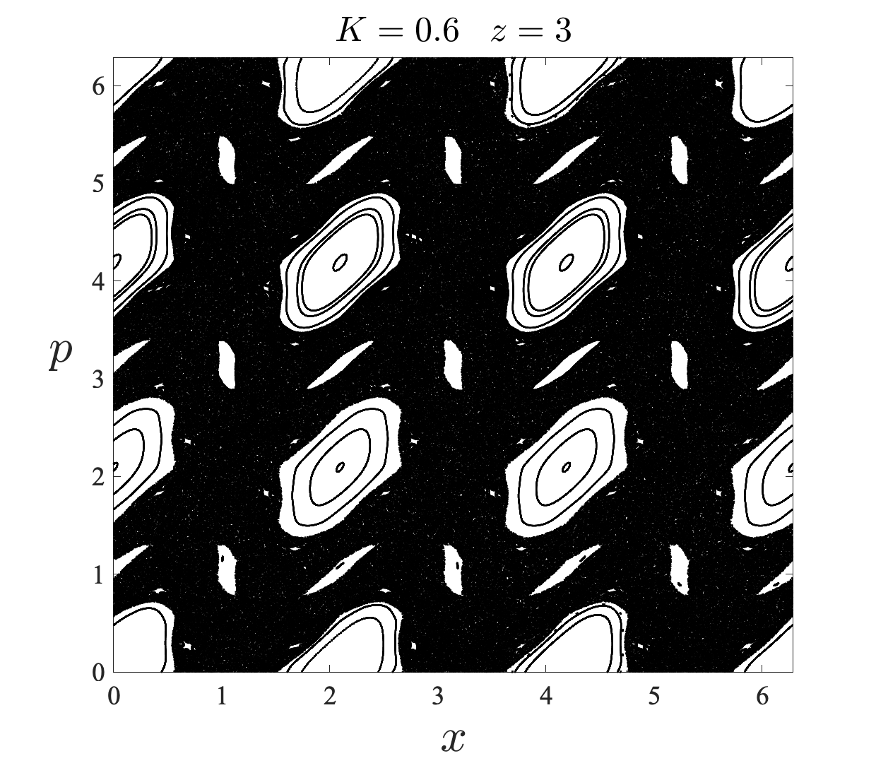
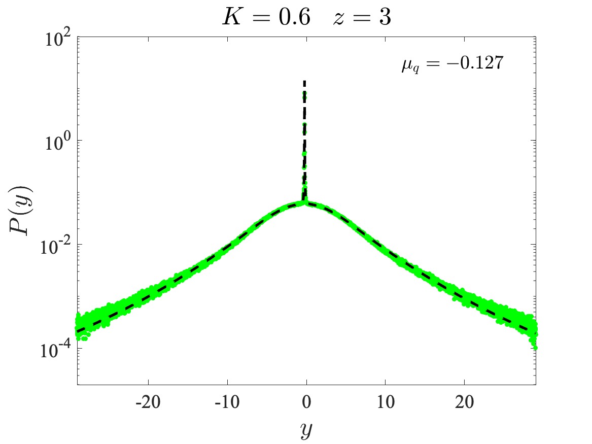
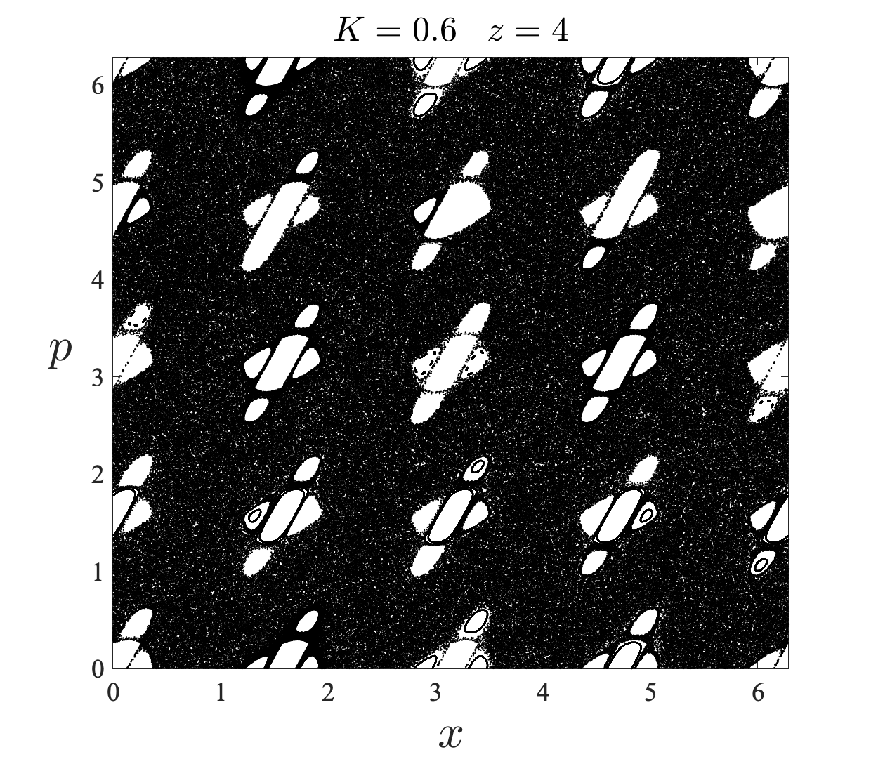
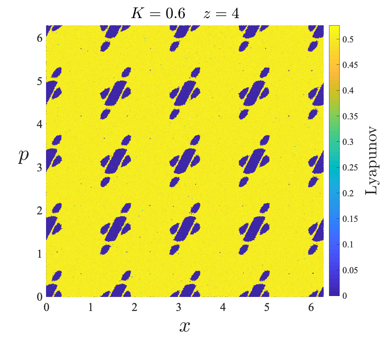
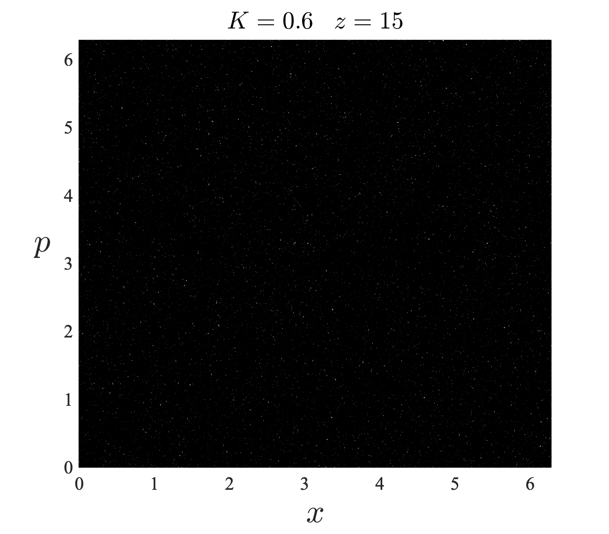
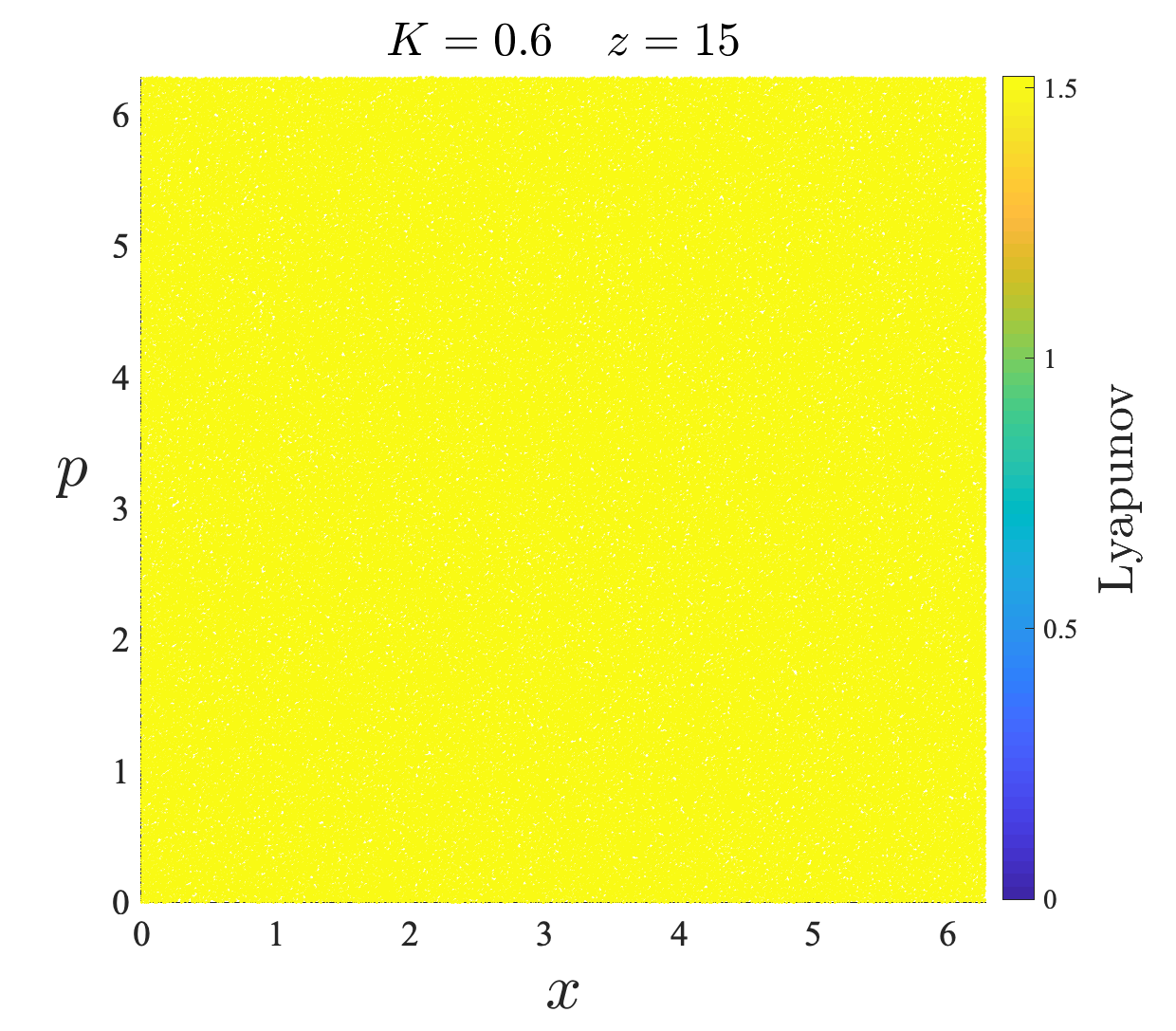
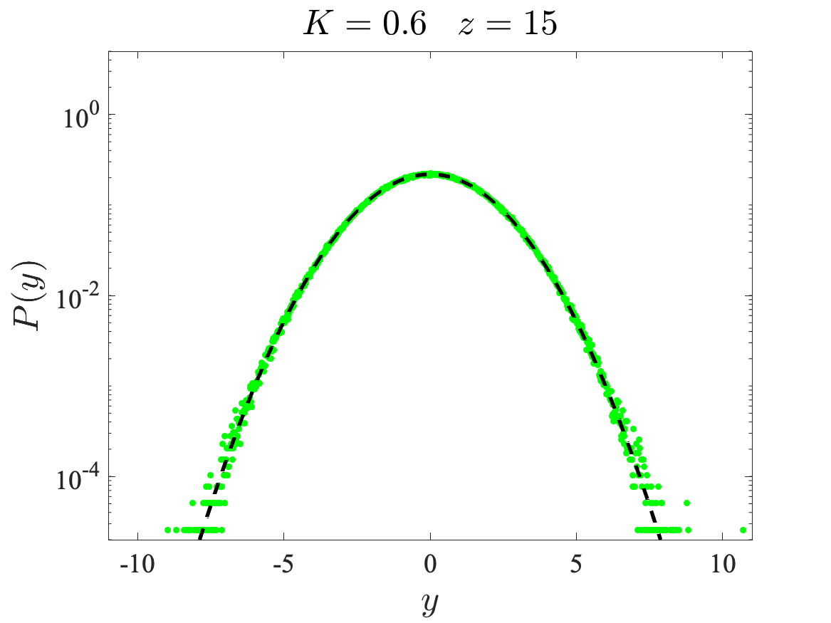
Figure 3: (Color online) Left column: Phase space portrait of the $z$-standard map for $K=0.6$ with various $z$ values; 40-50 initial conditions have been used in each case. Middle column: Lyapunov diagrams of the same cases. The Lyapunov exponents have been calculated over 500000 time steps using 500000 initial conditions taken randomly from the entire phase space. Right column: Probability distributions obtained for the same cases. In all cases, the number of initial conditions is larger than $3\times 10^{7}$ in order to achieve good statistics.

We come across with a more complicated limit behavior for the other parameter values of the generalized systems with $K=0.2$ and $K=0.6$ cases. Even though the phase spaces of these systems, given in Fig. 2 and Fig. 3, consist of both stability islands and the chaotic sea similar to the original standard case, the obtained limit distributions exhibit three-component behavior which can be modeled by Eq. 12. For each system mentioned above, relevant parameter values of probability distributions, shown in Fig. 2 and Fig. 3, are given in Table. 2. We see that unexpected third component is obtained as a $q$-Gaussian with different $q$ values for ($K=0.2$, $z=3$), ($K=0.6$, $z=3$) and ($K=0.6$, $z=4$) cases. More surprisingly, obtained probability distribution of ($K=0.2$, $z=5$) case consists of three $q$-Gaussians. In order to explain these interesting observations, we have to focus on the requirements for the occurrence of the $q$-Gaussians and the phase space behavior of the $z$-generalized standard map.

With the present $z$-generalization, we actually create systems with different phase space behavior. As it can be seen from the phase spaces given in Fig. 2 and Fig. 3, for typical values of $K$, increment of $z$ term increases the amount of nonintegrability of the system and chaotic behavior may occur for smaller $K$ values compared to the original standard map case. With the increasing nonintegrability Hilborn , the stability islands which are actually survived KAM tori dissolve according to the KAM theorem Arnold1978 and the Poincaré-Birkhoff theorem Birkhoff1935 .

According to the Poincaré-Birkhoff theorem, as a result of the resonances arisen with increased nonintegrability, each torus dissolves into alternating sequence of hyperbolic-elliptic points series depending on its winding number. Elliptic orbits occur around each elliptic point and in-sets and out-sets of hyperbolic points surround these elliptic orbits. Each elliptic-hyperbolic points series and in-sets and out-sets of hyperbolic points constitute a resonance. As the nonintegrability increases, resonances begin to overlap and destroy surviving tori that were in the region between them Hilborn . Chaotic behavior occurs with complex tangle structures created by in-sets and out-sets of the hyperbolic points. Homoclinic and heteroclinic tangles surround the elliptic orbits without intersecting them and a chaotic trajectory spread throughout this tangle structure by exhibiting mixing behavior Schuster . Dissolution of tori and enlarging chaotic behavior create archipelagos centered around the elliptic points in the phase space. Outer stability islands of the archipelagos continue to dissolve according to the KAM theorem and the Poincaré-Birkhoff theorem and chaotic behavior occupies larger portion of the phase space. It is important to note that this formation can be used to explain the occurrence of chaotic behavior in Hamiltonian systems and chaotic sea observed in the phase space corresponds to a single constant energy region of the Hamiltonian. By considering the resonance structure discussed above, we can conclude that complex homoclinic and heteroclinic tangles should stick around the elliptic orbits. This sticky behavior exists in the original standard map but chaotic trajectories spend less time in these sticky regions before escaping into the chaotic sea where they can wander throughout apparently randomly. When we modify the sine term in standard map as given in Eq. 10, we radically change the resonance behaviors and alternating sequence of hyperbolic-elliptic points series observed in the original case. As it can be seen from archipelagos in Fig. 2 and Fig. 3, each generalized system has different elliptic-hyperbolic points organization with periodicity related to the $z$ term in sine function. Starting from the integrable case, the case that is common for all $z$ values, tori located in resonance structures dissolve because of the overlaps. Sine term of the generalized standard map affects the number of hyperbolic-elliptic points and their positioning in the phase space and as a result of this effect resonances become stronger with increasing $z$ term for a constant $K$ value. Thus, more in-sets and out-sets of hyperbolic points create more complex tangle structures around stability islands. As these tangles tend to surround and stick around the stability islands, with more complicated structure chaotic trajectories spend more time for covering these tangle structures. Even though these sticky regions are connected to strongly chaotic sea, can be seen clearly from Fig. 2 and Fig. 3, an initial condition starting from the sticky region may spend most of its time in that region and may escape into the strongly chaotic sea after unpredictable time steps. Statistical effectiveness of sticky regions is presented in the probability distributions obtained for $z>1$ systems, i.e. especially for ($K=0.2$, $z=5$) case which explained in detail below. A chaotic trajectory should visit both chaotic sea and each sticky region, because the chaotic sea we see in the phase space is actually an allowed energy surface of the original Hamiltonian system which is created by dissolution of the constant energy surface tori. As a chaotic trajectory wanders throughout the allowed energy region apparently randomly, its behavior displays a mixing property and the system is said to be ergodic in that region.

When the phase space is fully occupied by the strongly chaotic sea, the whole system is ergodic and Gaussian distributions are obtained, which indicates the validity of the BG statistical framework. On the contrary, as a consequence of the ergodicity breakdown, $q$-Gaussians are appropriate distributions that describe the whole system with phase-space entirely occupied by stability islands. As these inferences are verified for the ($K=0.2$, $z=1$), ($K=0.2$, $z=40$) and ($K=0.6$, $z=15$) systems, two-component linear combinations of probability distributions of the ($K=0.6$, $z=1$) system shows that $q$-Gaussians arise from the initial conditions selected from stability islands whereas the Gaussian contribution comes from chaotic trajectories. It is important to note here that ergodicity breakdown alone is not sufficient for the occurrence of the $q$-Gaussians; indeed, special type of correlations among random variables are also needed. These requirements are fulfilled for stability islands of area-preserving maps Tirnakli, (2016); Ruiz, (2017); Ruiz2017b and, for chaotic bands, of band-splitting structure that approaches the chaos threshold of the dissipative logistic map by means of a Huberman-Rudnick-like scaling law ugur2007 ; ugur2009 ; Afsar2013 .

We see from Table 2 that the same $q$-Gaussian contributions with $q=1.935\pm 0.005$ come for each system. By taking into consideration that the same distribution is obtained for initial conditions selected from the stability islands of the original standard map ($z=1$) with different parameter values Tirnakli, (2016); Ruiz, (2017), we distinguish stability islands from the phase space by using the Lyapunov diagrams given in Fig. 2 and Fig. 3. Moreover, we verify that the phase-space occupation ratios of the stability islands of each case are exactly the $\alpha_{q_{1}}$ values given in Table 2. If the initial conditions from the stability islands are discarded, we are left with the chaotic sea in the phase space which should be related to the remaining components of the probability distribution given in Eq. 12. Let us start by analyzing the ($K=0.2$, $z=3$), ($K=0.6$, $z=3$) and ($K=0.6$, $z=4$) cases whose chaotic seas give rise to both a Gaussian and a $q$-Gaussian. When we look at the chaotic seas in the phase spaces of these systems in more detail, we see that strongly sticky regions which cannot occur in the original standard map arise for all these systems. Due to the resonance behaviors mentioned above, these sticky regions surround archipelagos and create complicated structures which are also connected with the chaotic sea. An initial condition located inside one of these sticky regions may give rise to a chaotic trajectory that stays inside this region for many iteration steps. An initial condition inside the sticky region evolves to cover this region, after unpredictable iteration steps, this trajectory may escape to the chaotic sea and may wander throughout the sea apparently randomly. In the probability distribution analyses, we use large but finite iteration steps and it seems that during this iteration steps chaotic trajectories located inside the sticky regions cannot display strong mixing behavior by confining inside these regions and not visiting large portion of the allowed energy region. Chaotic trajectories that do not enter sticky regions for large iteration steps can freely wander in the large portion of the allowed energy region and give rise to a Gaussian distribution. In principle, if it was possible to leave the system to evolve infinitely, the entire equal energy region would be covered by a single chaotic trajectory. In our observation interval, as some of the chaotic trajectories wander freely, some of them instead spend most of their times in the sticky region. Most probably, this observation may be a plausible explanation of the obtained limit probability distributions of systems that we investigate here. Observations made for the ($K=0.2$, $z=5$) case present more complicated scenario. When we look at the Lyapunov spectrum of this case in Fig. 2, we see the horizontal band-like structures. Based on our observations, the chaotic sea of each band acts as a sticky region in the phase space and all these regions are connected by not having any stability island as a barrier between them. When we analyze the phase space behavior of the chaotic trajectories by selecting initial conditions inside the chaotic seas and letting them to evolve, we observe that chaotic trajectories do not spread into the allowed energy region randomly as expected from the regular chaotic trajectory like we see in ($K=0.2$, $z=40$) and ($K=0.6$, $z=15$) systems. Instead of spreading into the allowed energy region randomly, chaotic trajectories first cover their bands’ chaotic sea and then move into another band. In our observations we see that even for large number of iteration steps, i.e. $T=10^{10}$, entire chaotic sea cannot be covered by a trajectory starting from an initial condition. As chaotic trajectories move in the phase space covering firstly one band and then the others respectively, mixing property of this system is completely different from that of the original system. This difference seems to be related to the occurrence of two $q$-Gaussian contributions detected for the limit probability distribution from the chaotic sea.

In order to improve our understanding of the emergence of the $q$-Gaussians, we have also analyzed the auto-correlation function $r_{\kappa}$ defined as follows

$$r_{\kappa}=\sum_{i=1}^{T-\kappa}\frac{(y_{i}-\langle y\rangle)(y_{i+\kappa}-\langle y\rangle)}{\sum_{i=1}^{T}(y_{i}-\langle y\rangle)^{2}}$$ (13)

where $\kappa$ is the time lag, $T$ is the number of iteration steps which constitute the trajectory, and $\langle y\rangle=T^{-1}\sum_{i=1}^{T}y_{i}$ MoralesNuevo1993 . Iterates of a trajectory are correlated for $r_{\kappa}\neq 0$ and not correlated for $r_{\kappa}=0$. For each system given in Table 2, we randomly choose a large number of initial conditions from the entire phase space and let the system to evolve along $T=2^{22}$ iteration steps, which coincides with the iteration number used in the probability distribution computations, starting from these initial conditions. In the computations of $r_{\kappa}$, for each trajectory, we use $\kappa=10^{5}$ as a maximum time lag by considering large computation times required for larger time lag values. Obtained results show that all systems exhibit three different tendencies for the auto-correlation function compatible with the probability distributions in the form of Eq. 12. In Fig. 4 and Fig. 5 we demonstrate the auto-correlation functions of the ($K=0.2$, $z=5$) and ($K=0.6$, $z=4$) systems as a function of the logarithm of the time lag respectively to corroborate the explanations given for nonergodic and nonmixing behavior of the chaotic trajectories. The logarithm of the time lag is used and $\kappa$ is cut at $10^{5}$ in order to obtain a better visualization of the oscillatory behavior of the auto-correlation functions. In both figures common green color is used to indicate the auto-correlation functions of iterates starting from initial conditions located inside one of the stability islands, e.g. ($x=5.042890762...$, $p=0.154394798...$­) for ($K=0.2$, $z=5$) system and ($x=1.617417044...$, $p=4.837677782...$­) for($K=0.6$, $z=4$) system. As seen from figures, green curve oscillates around zero with very large amplitudes and this behavior indicates that the iterates in the stability islands are strongly correlated. In Fig. 4 we see that red and black curves also oscillate around zero with different amplitudes that are smaller than the amplitude of the green one. Both of these functions are obtained for trajectories whose initial conditions are selected from the chaotic sea of the phase space, i.e. ($x=3.190574110......$, $p=7.259267286...\times 10^{-2}...$) for red and ($x=3.096157726...$, $p=9.095801865...\times 10^{-2}...$) for black. These auto-correlation function behaviors are three main types of correlations that are observed in the analyses of the ($K=0.2$, $z=5$) system and through this observations we can say that the chaotic trajectories in the phase space exhibit correlated behavior which is weaker than the correlation among the iterates of a trajectory in the stability islands. These three type of correlations observed in the phase space together with the nonergodicity of the present system mentioned above fulfill the requirements of the occurrence of the $q$-Gaussians and are thought to explain the obtained limit probability distribution which is a linear combination of three $q$-Gaussians. In Fig. 5 red and black curves are obtained for the initial conditions chosen from the chaotic region in the phase space. As initial condition ($x=5.654566893...$, $p=1.627640289...$) of red curve is located in the sticky region, ($x=5.668539896...$, $p=4.509105458...$) initial condition of black curve is located in the strongly chaotic sea. When we look at the figure, we see that black curve decreases to zero after a short time lag and oscillates around zero by indicating uncorrelated nature of the iterates of the trajectory. This auto-correlation function behavior is similar to the auto-correlation function obtained for the white noise which recently shown in Ref.Cetin2015 . On the contrary, red curve oscillates around zero with large amplitudes like the previous scenario. From these observations we can deduce that chaotic trajectories located inside the sticky regions may show correlations and chaotic trajectories that do not enter into the sticky regions for a long period of iteration steps display expected uncorrelated behavior of the chaotic trajectories. Also, we obtain the same auto-correlation function behaviors for ($K=0.2$, $z=3$) and ($K=0.6$, $z=3$) systems that exhibits similar limit probability distribution like ($K=0.6$, $z=4$) system. These observations seem to provide an adequate explanation for the obtained limit probability distributions.

Figure 4: (Color online) Three types of auto-correlation functions obtained for the $K=0.2$, $z=5$ case. The green curve is a representative result for a trajectory produced from an initial condition taken from the stability island (corresponding to a $q$-Gaussian with $q=1.935\pm 0.005$). The red and black curves are two representative results from trajectories started from the chaotic sea (corresponding to Gaussians with different $B$ values). Nonvanishing character of all auto-correlation functions is evident here.

Figure 5: (Color online) Three types of auto-correlation functions obtained for the $K=0.6$, $z=4$ case. The green curve is a representative result for a trajectory produced from an initial condition taken from the stability island (corresponding to a $q$-Gaussian with $q=1.935\pm 0.005$). The red and black curves are two representative results from trajectories started from the chaotic sea (corresponding to a $q$-Gaussian with $q\simeq 1.61$ and a Gaussian, respectively). Nonvanishing character of auto-correlation function is seen for one of them (red curve) which belongs to a trajectory of an initial condition that spends considerable time in the sticky region. Vanishing of the auto-correlation function for an initial condition (black curve) that does not enter the sticky regions is also evident.

V Conclusions

In this work, our results on the area-preserving maps can be summarized by classifying them into two groups: observations for the stability islands and for the chaotic trajectories. For the Harper map and several $z$-generalized standard map systems, for large number of iteration steps, the limit probability distributions coming from the sum of the iterates when the system is started from initial conditions located inside the stability islands seem to converge to a $q$-Gaussian with $q=1.935\pm 0.005$ value. Each different $z$ value corresponds to a new area-preserving system. Taking into account all of the maps analyzed in this paper and also results of the recent paper on the statistical characterization of the area-preserving web map Ruiz2017b , the main goal of this manuscript is to verify numerically that the limit probability distribution obtained when the system is initiated from initial conditions located in the stability islands is always well approximated by a $q$-Gaussian with $q=1.935\pm 0.005$ value. Regardless of the magnitude of the phase space occupation ratios of the stability islands (these ratios are not fitting parameters since they come directly from the Lyapunov spectrum of the system) for various map parameter values, $q$-Gaussian with $q=1.935\pm 0.005$ maintains its presence together with other distributions and this fact indicates that $q$-Gaussian with $q=1.935\pm 0.005$ value is a robust limit behavior for the stability islands of the area-preserving maps.

Although the stability islands of the area-preserving maps exhibit the same limit behavior, unexpected observations are made for chaotic trajectories of the different maps. Considering the definitional properties of the chaotic trajectories, e.g. the apparently random behavior and the exponential divergence of initially nearby trajectories, one can suggest that the chaotic trajectories wander freely through the allowed energy region and they spread into this region by displaying the mixing property. Under normal circumstances, a single chaotic trajectory rapidly spreads into allowed region and outlines this region after a few iteration steps. This common behavior of the chaotic trajectories is observed for all control parameter values of the Harper map. For all cases of the Harper map, when the chaotic region develops, we obtain Gaussian distributions for the limit behavior of the sums of the iterates for the initial conditions started from the chaotic sea, as expected. However, as shown here, some chaotic trajectories cannot exhibit regular behavior of the chaotic trajectories due to the sticky regions occur around stability islands for some area-preserving maps. Such a chaotic trajectory may not visit most of the allowed energy region during the observation time and therefore it cannot behave similarly as the chaotic trajectories which do not visit sticky regions during the same period of time. Even though chaotic trajectories exponentially diverge while covering the sticky region, magnitude of their divergence is much smaller compared to the divergence in the chaotic sea as seen from the Lyapunov spectra. A second $q$-Gaussian is obtained in limit probability distributions of systems that exhibit sticky behavior in their phase spaces and this might be explained due to different mixing property compared to the standard case and correlated nature of chaotic trajectories of sticky region. Even though contribution ratios of these second $q$-Gaussians cannot be determined directly from the Lyapunov spectra as we did before, they are thought to be as robust as other distributions that make contributions to the limit behavior for long but finite time intervals.

References

- (1) S. Umarov, C. Tsallis, S. Steinberg, Milan J. Math. 76 (2008) 307.
- (2) S. Umarov, C. Tsallis, M. Gell-Mann, S. Steinberg, J. Math. Phys. 51 (2010) 033502.
- (3) K.P. Nelson, S. Umarov, Physica A 389 (2010) 2157.
- (4) C. Vignat, A. Plastino, J. Phys. A 40 (2007) F969.
- (5) S. Umarov, C. Tsallis, Phys. Lett. A 372 (2008) 4874.
- (6) M.G. Hahn, X.X. Jiang, S. Umarov, J. Phys. A 43 (2010) 165208.
- (7) C. Tsallis, J. Stat. Phys. 52 (1988) 479.
- (8) C. Tsallis, Introduction to Nonextensive Statistical Mechanics - Approaching a Complex World (Springer, New York, 2009).
- Tirnakli, (2016) U. Tirnakli and E. P. Borges, Sci. Rep. 6 (2016) 23644.
- Ruiz, (2017) G. Ruiz, U. Tirnakli, E. P. Borges and C. Tsallis, J. Stat. Mech. 063403 (2017).
- (11) G. Ruiz, U. Tirnakli, E. P. Borges and C. Tsallis, Phys. Rev. E 96 (2017) 042158.
- (12) R. C. Hilborn, Chaos and nonlinear dynamics: An introduction for scientists and engineers (Oxford University Press, New York, 2000).
- (13) B. V. Chirikov, Proc. R. Soc. Lond. A 413 (1987) 145.
- (14) D. L. Shepelyansky and A. D. Stone, Phys. Rev. Lett. 74 (1995) 2098.
- (15) F. M. Izraelev, Physica D 1 (1980) 243.
- Zaslavsky, (1991) G. M. Zaslavsky, R- Z. Sagdeev, D. A. Usikov and A. A. Chernikov, Weak Chaos and Quasi-Regular Patterns (Cambridge Nonlinear Science Series, 1991).
- (17) P. Leboeuf, Physica D 116 (1998) 8.
- (18) G. Benettin, D. Casati, L. Galgani, A. Giorgilli and L. Sironi, Phys. Lett. A 118 (1986) 325.
- (19) U. Tirnakli, C. Beck and C. Tsallis, Phys. Rev. E 75 (2007) 040106(R).
- (20) U. Tirnakli, C. Tsallis and C. Beck, Phys. Rev. E 79 (2009) 056209.
- (21) O. Afsar and U. Tirnakli, EPL 101 (2013) 20003.
- (22) K. Cetin, O. Afsar and U. Tirnakli, Physica A 424 (2015) 269.
- (23) D. Prato and C. Tsallis, Phys. Rev. E 60 (1999) 2398.
- (24) C. E. E. Karney, Phys. Fluids 22 (1979) 2188.
- (25) P. Lebeuf, J. Kurchan, M. Feingold and D. P. Arovas, Phys. Rev. Lett. 65 (1990) 3076.
- (26) R. A. Pasmanter, Phys, Rev. A 42 (1990) 3622.
- (27) G. M. Zaslavsky, The Physics of Chaos in Hamiltonian Systems (Imperial College Press, London, 1979).
- (28) B. V. Chirikov, Phys. Rep. 52 (1979) 263.
- (29) V. I. Arnold, Mathematical Methods in Classical Mechanics (Springer, New York, 1978).
- (30) G. D. Birkhoff, Pont. Acad. Sci. Novi Lyncaei, 1, 85 (1935).
- (31) H. G. Schuster and W. Just, Deterministic Chaos: An Introduction (Wiley-VCH, Weinheim, 2005).
- (32) J. J. Morales and M. J. Nuevo, Phys. Rev. E 48 (2), 1550 (1993).