A Conformal Dispersion Relation:
Correlations from Absorption

Abstract

We introduce the analog of Kramers-Kronig dispersion relations for correlators of four scalar operators in an arbitrary conformal field theory. The correlator is expressed as an integral over its “absorptive part”, defined as a double discontinuity, times a theory-independent kernel which we compute explicitly. The kernel is found by resumming the data obtained by the Lorentzian inversion formula. For scalars of equal scaling dimensions, it is a remarkably simple function (elliptic integral function) of two pairs of cross-ratios. We perform various checks of the dispersion relation (generalized free fields, holographic theories at tree-level, 3D Ising model), and get perfect matching. Finally, we derive an integral relation that relates the “inverted” conformal block with the ordinary conformal block.

1 Introduction

The conformal bootstrap has enjoyed remarkable success in the last decade, employing both numerical Rattazzi:2008pe ; ElShowk:2012ht ; Simmons-Duffin:2016wlq ; Poland:2018epd and analytic Komargodski:2012ek ; Fitzpatrick:2012yx ; Alday:2015ewa ; Alday:2016njk methods to solve general consistency conditions. Some of the primary methods of the analytic bootstrap include: light-cone expansions of the crossing equations, large $N$ expansions, AdS/CFT, and causality constraints.

Implications of causality are often effectively captured by dispersion relations, following the work of Kramers and Kronig in optics. These authors related (in 1926) the dispersive (real) and absorptive (imaginary) part of the index of refraction, exploiting analyticity of the index of refraction in the upper-half complex frequency plane. Dispersion relations were later used to try and constrain the relativistic S-matrix Martin:1969ina ; Eden1 ; Screaton . This was an important tool for physicists in the 1950’s and 60’s who, in the absence of a microscopic theory, attempted to solve or “bootstrap” the strong interactions using consistency with the principles of causality, unitarity, and crossing; a program which waned down at the time with the advent of QCD as a microscopic description of the strong force.

Dispersion relations are typically most useful when one knows more about the absorptive part than the real part. For the strong force at low energies, the imaginary part is often saturated by narrow resonances, leading to phenomenologically interesting sum rules Shifman:1992xu . It may also happen that the imaginary part (or the absolute value of the amplitude) is the only quantity measured experimentally. Theoretically, the imaginary part enjoys useful properties such as positivity (for example in the forward limit), related to probabilities being nonnegative; applications include the first proof of irreversibility of renormalization group flow in four spacetime dimensions Komargodski:2011vj . In perturbative scattering amplitudes, absorptive parts can be efficiently computed in terms of lower-order amplitudes through the Cutkosky rules, a foundational insight that is now built into successful methods such as generalized unitarity Bern:1994zx ; Britto:2004nc ; Britto:2005fq ; Elvang:2013cua . Given that crossing symmetry and general principles appear to be particularly powerful in conformal field theories, it is natural to expect a CFT dispersion relation to be a useful tool in constraining CFT correlators.

In this paper we derive a dispersion relation for CFT 4-point correlators $\mathcal{G}(z,{\bar{z}})$:

$$\boxed{\mathcal{G}^{t}(z,{\bar{z}})=\int_{0}^{1}dwd{\bar{w}}K(z,{\bar{z}},w,{\bar{w}}){\rm dDisc}[\mathcal{G}(w,{\bar{w}})]}$$ (1)

where we separate the $t$ and $u$ channel contributions and a possible finite sum of non-normalizable blocks (see section 4.2.1):

$$\mathcal{G}(z,{\bar{z}})=\mathcal{G}^{t}(z,{\bar{z}})+\mathcal{G}^{u}(z,{\bar{z}})+\mbox{(non-norm.)}\,.$$ (2)

The input ${\rm dDisc}[\mathcal{G}(z,{\bar{z}})]$ represents the double-discontinuity of the correlator around ${\bar{z}}=1$, defined below, and is interpreted physically as its absorptive part. We notice that the correlator is a function of two cross-ratios $(z,{\bar{z}})$: the kernel $K(z,{\bar{z}},w,{\bar{w}})$ is thus a function of two pairs of cross-ratios, one pair being integrated over (with $w,{\bar{w}}$ real in the integration region). This is to be contrasted with more familiar Kramers-Kronig type dispersion relations, in which a single variable is integrated over. We will argue that such a complication is unavoidable if we insist that the input be the “absorptive part” ${\rm dDisc}[\mathcal{G}]$, as the analytic properties of the correlators $\mathcal{G}(z,{\bar{z}})$ entangle its two arguments.

The existence of a formula such as (1), reconstructing correlators from (double) discontinuities, is suggested by the Lorentzian inversion formula of Caron-Huot:2017vep ; Simmons-Duffin:2017nub ; Kravchuk:2018htv . That formula reconstructs operator product expansion data from knowledge of the discontinuities ${\rm dDisc}[\mathcal{G}(z,{\bar{z}})]$ of the CFT 4-point correlator, and has been used notably to streamline light-cone and large-$N$ expansions. Examples suggest that a crude approximation to the ${\rm dDisc}$ (ie. including the simplest few exchanged operators) can lead to accurate results to the OPE data itself. These examples range from the low-twist spectrum in 3D Ising and related models Alday:2017zzv ; Alday:2019clp ; Albayrak:2019gnz ; Cardona:2018qrt ; Li:2019dix , mean field theory Liu:2018jhs , the calculation of Witten diagrams in strongly coupled (holographic) gauge theories Alday:2017vkk ; Caron-Huot:2018kta , as well as defect CFTs and certain finite temperature effects Lemos:2017vnx ; Iliesiu:2018fao .

We find it is extremely encouraging that good first approximations to the dDisc are easy to come by. This begs the question of systematic improvement. One limitation of the Lorentzian inversion formula is that it is difficult to iterate it. For example, its output cannot simply be fed back into it, in a way that would lead to successively better approximations (while the formula produces a generating function for the spectrum, computing the dDisc requires resolving the dimensions of individual operators, a step which requires a numerically difficult analytic continuation). The dispersion relation (1) offers a step forward, since it enables crossing equations to be formulated directly on the positive dDisc. As we will see, it will also circumvent technical limitations regarding convergence at low spins.

In this paper we derive the dispersion relation (1), and in particular the kernel $K$ entering it, by resumming the OPE data extracted via the Lorentzian inversion formula. The result can be split into a two-dimensional bulk integral $K_{B}$ and a one-dimensional contact integral $K_{C}$:

$$K(z,{\bar{z}},w,{\bar{w}})=K_{B}\theta(\rho_{z}{\bar{\rho}_{z}}{\bar{\rho}_{w}}-\rho_{w})+K_{C}\frac{d\rho_{w}}{dw}\delta(\rho_{w}-\rho_{z}{\bar{\rho}_{z}}{\bar{\rho}_{w}})$$ (3)

where $\theta(x)$ is the unit step function and $\delta(x)$ is the Dirac $\delta$-function. In the case of operators of equal external scaling dimensions, our main result is the explicit form:

$$\begin{aligned} K_{B}&=-\frac{1}{64\pi}\left(\frac{z{\bar{z}}}{w{\bar{w}}}\right)^{3/2}\frac{({\bar{w}}-w)(\frac{1}{w}+\frac{1}{{\bar{w}}}+\frac{1}{z}+\frac{1}{{\bar{z}}}-2)}{((1-z)(1-{\bar{z}})(1-w)(1-{\bar{w}}))^{\frac{3}{4}}}\ x^{\frac{3}{2}}{}_{2}F_{1}(\tfrac{1}{2},\tfrac{3}{2},2,1-x),\\ K_{C}&=\frac{4}{\pi}\frac{1}{{\bar{w}}^{2}}\left(\frac{1-\rho_{z}^{2}{\bar{\rho}_{z}}^{2}{\bar{\rho}_{w}}^{2}}{(1-\rho_{z}^{2})(1-{\bar{\rho}_{z}}^{2})(1-{\bar{\rho}_{w}}^{2})}\right)^{1/2}\frac{1-\rho_{z}{\bar{\rho}_{z}}{\bar{\rho}_{w}}^{2}}{(1-\rho_{z}{\bar{\rho}_{w}})(1-{\bar{\rho}_{z}}{\bar{\rho}_{w}})}.\end{aligned}$$ (4)

The first involves a rather special combination of cross ratios:

$$x\equiv\frac{\rho_{z}{\bar{\rho}_{z}}\rho_{w}{\bar{\rho}_{w}}(1-\rho_{z}^{2})(1-{\bar{\rho}_{z}}^{2})(1-\rho_{w}^{2})(1-{\bar{\rho}_{w}}^{2})}{({\bar{\rho}_{z}}{\bar{\rho}_{w}}-\rho_{w}\rho_{z})(\rho_{z}{\bar{\rho}_{w}}-\rho_{w}{\bar{\rho}_{z}})(\rho_{z}{\bar{\rho}_{z}}-\rho_{w}{\bar{\rho}_{w}})(1-\rho_{w}\rho_{z}{\bar{\rho}_{w}}{\bar{\rho}_{z}})}.$$ (5)

The bulk integral contributes only for $\rho_{w}<\rho_{z}{\bar{\rho}_{w}}{\bar{\rho}_{z}}$ (due to the step function), and is proportional to a hypergeometric function, which can equivalently be written as a combination of elliptic integral functions, see eq. (54). The contact integral, proportional to a $\delta$-function, is effectively integrated over a single variable ${\bar{w}}\in[0,1]$. An alternative but equivalent form, which unites the bulk and contact terms, is given in eq. (84).

We find it remarkable that a function of four complex variable can be written in closed form as in eq. (4). As we will see in section 4, each factor plays a role, and $K$ above is arguably the simplest possible kernel able to fulfil the difficult task assigned to it.

The outline of the paper is as follows. In section 2.1 we review the amplitude dispersion relation and the Froissart-Gribov inversion formula, and how one can derive the former from the latter. This exercise will prepare us for the more difficult case of the CFT dispersion relation. In section 3 we show the full details of derivation of the CFT dispersion relation in $d=2$ for scalars with equal external scaling dimensions. We obtain an analytic result for the kernel, in terms of elliptic integral functions. The same kernel is valid in any dimension, and we show that in section 3.3 that indeed repeating the calculation in $d=4$ yields the same kernel. In section 3.4 we derive the dispersion relation for unequal external scaling dimension. The kernel satisfies a differential equation, giving Taylor expansions for it. For a specific simple case, $a=0$ and $b=\frac{1}{2}$, we also find an analytic form for the kernel. In section 4 we establish the validity of the dispersion relation by a direct contour deformation argument. This allows to overcome some of the original assumptions, and in particular we obtain a subtracted dispersion relation that is valid in any unitary CFT. In section 5 we explore possible applications of the dispersion relation: to strong coupling $\mathcal{N}=4$ SYM, to obtain novel identities relating inverted and conformal blocks, and to the 3D Ising model and new bootstrap functionals. We conclude by discussing future directions in section 6.

Note added: While this paper was being completed, the work Bissi:2019kkx appeared on arxiv who introduced a single-variable dispersion relation that reconstructs correlators from a single-discontinuity. This appears to be quite distinct from the formulas considered here: the input in this case (to our knowledge) is neither sign-definite nor admits a physical interpretation as an absorptive part.

2 Preliminaries

2.1 Review of amplitude dispersion relation

Dispersion relations enable to construct a function from a knowledge of it’s discontinuities. The most common type of a dispersion relation is the single variable dispersion relation, where one variable is being integrated over. For definiteness, we will discuss this here in the context of the relativistic 4-particle scattering amplitude, although the reader may wish to keep in mind that the construction is more general. We will review two derivations, the first involving a contour deformation argument which is perhaps the most familiar.

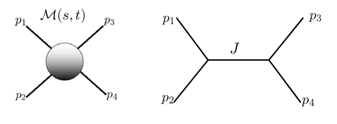
Figure 1: Left: The 4-particle scattering amplitude $\mathcal{M}(s,t)$, with external momenta $p_{i}$. Right: $t$-channel tree level exchange diagram of particle with spin $J$ .

Consider the 4-particle scattering amplitude $\mathcal{M}(s,t)$ for scalars with mass $m$ (fig. 1 left). $\mathcal{M}(s,t)$ is a function of the two Mandelstam variables $s\equiv-(p_{1}+p_{2})^{2}$ and $t\equiv-(p_{1}-p_{3})^{2}$, with the energy conservation constraint $s+t+u=4m^{2}$. For $s$ constant and in a suitable range, the complex $t$-plane has the structure depicted in fig. 2, with two branch cuts along the real axis for $t>t_{0}$ and $t<4m^{2}-s-t_{0}$. These are called the $s$- and $t$-channel cuts (the second condition corresponding to $u>u_{0}$). The single variable dispersion relation to be considered is:

$$\mathcal{M}(s,t)=\frac{1}{2\pi}\int_{t_{0}}^{\infty}\frac{dt^{\prime}}{t^{\prime}-t}{\rm Disc}_{t^{\prime}}[\mathcal{M}(s,t^{\prime})]+(t\leftrightarrow u)$$ (6)

The integral runs over the branch cuts of $\mathcal{M}(s,t^{\prime})$, and $i\ {\rm Disc}_{t^{\prime}}[\mathcal{M}(s,t^{\prime})]\equiv\mathcal{M}(s,t^{\prime}+i0)-\mathcal{M}(s,t^{\prime}-i0)$ is the discontinuity across the cuts in the $t^{\prime}$-plane. Note that the variable $s$ just goes along for the ride.

$$\begin{array}[]{cc}\end{array}&\hskip 17.07164pt\raisebox{48.36967pt}{\leavevmode\resizebox{19.91692pt}{}{$\Rightarrow$}}\hskip 17.07164pt\begin{picture}(1.0,0.54366)\put(0.75727,0.20182){\color[rgb]{0,0,0}\makebox(0.0,0.0)[lb]{\smash{ }}}\put(0.0,0.0){\includegraphics[width=193.47873pt,page=1]{dispersion2.pdf}}\end{picture}$$

Figure 2: Left: The amplitude can be written as a contour integral by using Cauchy’s theorem. Right: Upon deforming the contour, there will be contributions from the branch cuts and from the arcs at infinity.

A common way to derive this is to start with a contour integral in the complex $t^{\prime}$ plane surrounding the point $t$ (see Fig 2); by Cauchy’s residue theorem:

$$\mathcal{M}(s,t)=\frac{1}{2\pi i}\oint\frac{dt^{\prime}}{t^{\prime}-t}\mathcal{M}(s,t^{\prime}).$$ (7)

Then one deforms the contour of integration as in Fig 2. If $\mathcal{M}(s,t^{\prime})$ decays fast enough at $|t^{\prime}|\to\infty$ that the arcs at infinity can be neglected, only the branch cuts contribute, reproducing eq. (6) as desired.

What if $\mathcal{M}(s,t^{\prime})$ does not decay fast enough? If it is polynomially bounded, one can still obtain a subtracted dispersion relation. The idea is to improve the behavior on large arcs by subtracting the amplitude at some reference $t=t_{*}$:

$$\mathcal{M}(s,t)-\mathcal{M}(s,t_{*})=\frac{1}{2\pi}\int_{t_{0}}^{\infty}dt^{\prime}\left[\frac{1}{t^{\prime}-t}-\frac{1}{t^{\prime}-t_{*}}\right]{\rm Disc}_{t^{\prime}}[\mathcal{M}(s,t^{\prime})]+\mbox{u-channel},$$ (8)

which has improved convergence since the bracket $\sim 1/|t^{\prime}|^{2}$. One can generalize by applying more subtractions as needed. A perhaps more illuminating way to write this is to use elementary algebra to rewrite the bracket as $\frac{t-t_{*}}{(t^{\prime}-t)(t^{\prime}-t_{*})}$, and divide both sides by $(t-t_{*})$; the once-subtracted dispersion relation (8) becomes:

$$\frac{\mathcal{M}(s,t)}{t-t_{*}}=\frac{1}{2\pi}\int_{t_{0}}^{\infty}\frac{dt^{\prime}}{t^{\prime}-t}\ {\rm Disc}_{t^{\prime}}\left[\frac{\mathcal{M}(s,t^{\prime})}{t^{\prime}-t_{*}}\right]+\mbox{u-channel}.$$ (9)

This is nothing but the original dispersion relation, now applied to the rescaled function $\mathcal{M}(s,t)/(t-t_{*})$. This viewpoint will be useful below.

In the amplitude context, the dispersion integral generally runs over unphysical regions of the $(s,t^{\prime})$-plane, where ${\rm Disc}_{t^{\prime}}\mathcal{M}$ is neither positive-definite nor physically measurable. An exception is for the range $0\leq s<4m^{2}$ in a theory with mass gap $m$: there the discontinuity is positive-definite, and is a smooth extrapolation (to imaginary angles) of physically measurable $t$- and $u$-channel scattering amplitudes. This is an important result of Martin, used in his celebrated proof of the Froissard bound on the high-energy growth of total cross-sections Martin:1962rt . The CFT dispersion relation discussed in this paper will share the nice features of this special region.

For more on applications of scattering amplitude dispersion relations, the reader may consult Martin:1969ina ; Eden1 ; Screaton . For a more recent application, see the following works on the S-matrix bootstrap Paulos:2016but ; Paulos:2017fhb .

2.1.1 Dispersion relation from the Froissart-Gribov formula

We turn to a perhaps less familiar derivation of the dispersion relation, starting from the Froissart-Gribov formula expressing partial wave coefficients from the discontinuity of the amplitude.

Consider the partial wave decomposition of the amplitude in the $s$-channel (Fig. 1 right), for definiteness working in $d=4$ dimensions:

$$\mathcal{M}(s,t(z))=\frac{1}{2}\sum_{J=0}^{\infty}(2J+1)a_{J}(s)P_{J}(z),\qquad z\equiv\cos\theta,\qquad t(z)=\frac{4m^{2}-s}{2}(1-z).$$ (10)

Physically, $\theta$ is the scattering angle and the coefficients $a_{J}(s)$ encode the decomposition of the amplitude into spherical harmonics at a given energy-squared $s$.

Using the orthogonality of the Legendre polynomials, $\int_{-1}^{1}dzP_{J^{\prime}}(z)P_{J}(z)=\frac{2\delta_{JJ^{\prime}}}{2J+1}$, one may readily obtain a “Euclidean inversion formula” expressing the coefficients as an integral over the amplitude. A less obvious formula, first derived by Froissart and Gribov Froissart ; Gribov , expresses the same data in terms of the discontinuity of the amplitude:

$$a_{J}^{t}(s)=\frac{1}{\pi}\int_{1}^{\infty}dz^{\prime}Q_{J}(z^{\prime})\ {\rm Disc}_{t}\mathcal{M}(s,t(z^{\prime})),\qquad a_{J}(s)=a_{J}^{t}(s)+(-1)^{J}a^{u}_{J}(s),$$ (11)

where $Q_{J}(z_{s}^{\prime})$ is the Legendre function of the second kind. $a_{J}^{t}(s)$ and $a_{J}^{u}(s)$ are the contributions from the $t$-channel and $u$-channel cuts respectively. The Frossart-Gribov formula plays a foundational role in Regge theory, as it establishes analyticity in spin of the partial waves (as well as providing quantitative large-spin estimates).

A proof of eq. (11) starts from the orthogonality relation, rewriting the integral over $z\in[-1,1]$ as a contour integral using that $P_{J}\propto{\rm Disc}\ Q_{J}$. One then deforms the contour exactly as in fig. 2 above (see Caron-Huot:2017vep for recent discussion with two derivations). The Froissart-Gribov formula and dispersion relation are thus closely related, and it should come as no surprise that one can derive either one from the other.

To go the other way, the trick is simply to plug the coefficient obtained from eq. (11) into the partial wave sum in eq. (10), and interchange the summation and integration:

$$\mathcal{M}(s,t(z))=\sum_{J=0}^{\infty}(2J+1)P_{J}(z)\frac{1}{2\pi}\int_{1}^{\infty}dz^{\prime}Q_{J}(z^{\prime}){\rm Disc}_{t}\mathcal{M}(s,t(z^{\prime}))+(t\leftrightarrow u)$$

$$=\frac{1}{2\pi}\int_{1}^{\infty}dz^{\prime}{\rm Disc}_{t}\mathcal{M}(s,t(z^{\prime}))\sum_{J=0}^{\infty}(2J+1)P_{J}(z)Q_{J}(z^{\prime})+(t\leftrightarrow u).$$ (12)

The latter sum then turns into the following identity (for $|z|<|z^{\prime}|$):

$$\sum_{J=0}^{\infty}(2J+1)P_{J}(z)Q_{J}(z^{\prime})=\frac{1}{z^{\prime}-z}$$ (14)

which is recognized as the kernel of the dispersion relation (6). (One needs only the change of variable $\frac{dz^{\prime}}{z^{\prime}-z}\mapsto\frac{dt^{\prime}}{t^{\prime}-t}$.)

We call the measure $\frac{dt^{\prime}}{t^{\prime}-t}$, which multiplies the discontinuity, the “kernel”. Interestingly, even though the form of the special functions $P_{J}$ and $Q_{J}$ changes in a complicated way as a function of spacetime dimension, and the left-hand-side of eq. (14) acquires a measure factor $[(1-z^{\prime 2})/(1-z)^{2}]^{(d-4)/2}$, one can show that the sum produces the same right-hand-side in any dimension. This was to be expected physically, since the dimension simply did not enter the earlier derivation anywhere.

The reader may wonder why one would want to derive a dispersion relation starting from the Froissart-Gribov formula (11), as opposed to simply writing down the more elementary Cauchy kernel $\frac{dt^{\prime}}{t^{\prime}-t}$. The reason is that the substitution $P_{J}\mapsto{\rm Disc}\ Q_{J}$ underlying the former has a group-theoretical explanation (ie. both functions satisfy the same Casimir differential equation), whereas writing down the Cauchy kernel requires an educated guess. For conformal correlators, the group-theoretic approach was successfully carried out in ref. Caron-Huot:2017vep , whereas the guessing approach turns out to be much more challenging.

2.2 Review of CFT kinematics

In this paper we will focus on a correlator of four scalar primary operators in a CFT. This can be written as a function of cross ratios $z$ and ${\bar{z}}$ multiplied by an overall factor which is determined by the conformal symmetry:

$$\langle\mathcal{O}_{1}(x_{1})\mathcal{O}_{2}(x_{2})\mathcal{O}_{3}(x_{3})\mathcal{O}_{4}(x_{4})\rangle=\frac{\Big{(}\frac{x^{2}_{14}}{x^{2}_{24}}\Big{)}^{a}\Big{(}\frac{x^{2}_{14}}{x^{2}_{13}}\Big{)}^{b}}{(x^{2}_{12})^{\frac{1}{2}(\Delta_{1}+\Delta_{2})}(x^{2}_{34})^{\frac{1}{2}(\Delta_{3}+\Delta_{4})}}\mathcal{G}(z,{\bar{z}})\,,$$ (15)

where we defined the differences of the external scaling dimensions:

$$a=\tfrac{1}{2}(\Delta_{2}-\Delta_{1}),\qquad b=\tfrac{1}{2}(\Delta_{3}-\Delta_{4})\,$$ (16)

and the cross ratios $z,{\bar{z}}$ are defined through:

$$u=z{\bar{z}}=\frac{x^{2}_{12}x^{2}_{34}}{x^{2}_{13}x^{2}_{24}}\ ,\qquad v=(1-z)(1-{\bar{z}})=\frac{x^{2}_{23}x^{2}_{14}}{x^{2}_{13}x^{2}_{24}}\ .$$ (17)

We will often use the so-called radial or $\rho$-coordinates of ref. Hogervorst:2013sma ,

$$\rho_{z}\equiv\frac{1-\sqrt{1-z}}{1+\sqrt{1-z}}\ ,\quad{\bar{\rho}_{z}}\equiv\frac{1-\sqrt{1-{\bar{z}}}}{1+\sqrt{1-{\bar{z}}}}\ ,\quad z=\frac{4\rho_{z}}{(1+\rho_{z})^{2}}\ ,\quad{\bar{z}}=\frac{4{\bar{\rho}_{z}}}{(1+{\bar{\rho}_{z}})^{2}}$$ (18)

which provide a double cover of the complex $z$-plane.

We will be focusing on the $s$-channel operator product expansion (OPE):

$$\mathcal{G}(z,{\bar{z}})=\sum_{J,\Delta}f_{12\mathcal{O}_{J,\Delta}}f_{43\mathcal{O}_{J,\Delta}}G_{J,\Delta}(z,{\bar{z}})$$ (19)

where $f_{ij\mathcal{O}}$ are the OPE coefficients and $G_{J,\Delta}(z,{\bar{z}})$ are $s$-channel conformal blocks for exchange of a primary operator with spin $J$ and scaling dimension $\Delta$, and its descendants. For our purposes the OPE may also be written as an integral over principal series representations (harmonic functions), in which the scaling dimension is continuous (see Dobrev:1975ru ; Dobrev:1977qv ; Costa:2012cb ):

$$\mathcal{G}(z,{\bar{z}})=\sum_{J=0}^{\infty}\int_{\frac{d}{2}-i\infty}^{\frac{d}{2}+i\infty}\frac{d\Delta}{2\pi i}c(J,\Delta)F_{J,\Delta}(z,{\bar{z}})+\mbox{(non-norm.)}.$$ (20)

The “non-normalizable” part includes the $s$-channel identity operator as well as a possible finite sum of $F$ functions for scalar operators with dimension less than $d/2$. The CFT data is then encoded in the poles of $c_{J,\Delta}$, which occur on the real axis of the complex $\Delta$ plane at the position of the physical scaling dimensions, and whose residue are the squared OPE coefficients:

$$f_{12\mathcal{O}_{J,\Delta}}f_{43\mathcal{O}_{J,\Delta}}=-{\rm Res}_{\Delta^{\prime}=\Delta}\big{[}c(J,\Delta^{\prime})\big{]}.$$ (21)

The $F$ stand for harmonic functions, which combine a block and its shadow

$$F_{J,\Delta}(z,{\bar{z}})=\frac{1}{2}\Big{(}G_{J,\Delta}(z,{\bar{z}})+\#G_{J,d-\Delta}(z,{\bar{z}})\Big{)},$$ (22)

with a specific coefficient that will not be important below. (It ensures that $F$ is single-valued in Euclidean space where ${\bar{z}}=z^{*}$, a necessary condition for the $F$’s to form a complete orthogonal basis.)

Using the orthogonality for $F_{J,\Delta}(z,{\bar{z}})$, one may readily write an Euclidean inversion formula expressing the OPE data $c_{J,\Delta}$ as an integral over correlators, in analogy to that for Legendre polynomials discussed below eq. (10). Instead we will use the Lorentzian inversion formula, which reconstructs the same data from an “absorptive part” Caron-Huot:2017vep ; Simmons-Duffin:2017nub ; Kravchuk:2018htv

$$c^{t}(J,\Delta)=\frac{\kappa_{J+\Delta}}{4}\int_{0}^{1}dwd{\bar{w}}\ \mu(w,{\bar{w}})\ G_{\Delta+1-d,J+d-1}(w,{\bar{w}})\ {\rm dDisc}[\mathcal{G}(w,{\bar{w}})]$$ (23)

where the integration region is the square $0\leq w,{\bar{w}}\leq 1$, the normalization and measure are

$$\kappa_{\beta}=\frac{\Gamma(\frac{\beta}{2}-a)\Gamma(\frac{\beta}{2}+a)\Gamma(\frac{\beta}{2}-b)\Gamma(\frac{\beta}{2}+b)}{2\pi^{2}\Gamma(\beta-1)\Gamma(\beta)},\qquad\mu(w,{\bar{w}})=\Big{|}\frac{w-{\bar{w}}}{w{\bar{w}}}\Big{|}^{d-2}\frac{((1-w)(1-{\bar{w}}))^{a+b}}{(w{\bar{w}})^{2}},$$ (24)

and the OPE data itself is the sum of $t$- and $u$-channel contributions (as in eq. (11)):

$$c(J,\Delta)=c^{t}(J,\Delta)+(-1)^{J}c^{u}(J,\Delta).$$ (25)

The $u$-channel contribution may be obtained by applying the integral (23) to the correlator with operators 1 and 2 swapped.

Notice that the conformal block $G_{\Delta+1-d,J+d-1}(w,{\bar{w}})$ appearing in the inversion formula above is not the usual block, it has the roles of $J$ and $\Delta$ reversed; we may call it the “inverted block”. (This reversal is a Weyl reflection of the so$(d,2)$ Lie algebra.) This is analogous to the substitution $P_{J}\mapsto Q_{J}$ in eq. (11). One can draw a close analogy between between 4-point CFT correlators and 4-particle amplitude scattering amplitudes, see Table 1.

The “${\rm dDisc}$” is primarily defined as a expectation value of the double-commutator $-\frac{1}{2}\langle 0|[O_{2},O_{3}][O_{1},O_{4}]|0\rangle$, divided by the normalization factor in eq. (15). It can be computed as a double discontinuity, or difference between three analytic continuations, around the point ${\bar{z}}=1$:

$${\rm dDisc}\ [\mathcal{G}(\rho,\bar{\rho})] \equiv \cos(\pi(a{+}b))\mathcal{G}(\rho,\bar{\rho})$$ (26)

$$-\tfrac{1}{2}e^{i\pi(a+b)}\mathcal{G}(\rho,\bar{\rho}^{-1}{-}i0)-\tfrac{1}{2}e^{-i\pi(a+b)}\mathcal{G}(\rho,\bar{\rho}^{-1}{+}i0)$$

where we assume $0<\rho,\bar{\rho}<1$. This represents a discontinuity since ${\bar{\rho}_{z}}$ and ${\bar{\rho}_{z}}^{-1}$ map onto the same cross-ratio ${\bar{z}}$, see eq. (18).

Physically, the dDisc is interpreted as an absorptive part because it represents one minus the survival probability of a certain state. In particular it is positive-definite by unitarity, see section 2.2 of Caron-Huot:2017vep . In holographic theories, the double discontinuity effectively puts bulk propagators on-shell (as seen in specific tree and one-loop examples, see ref. Alday:2017vkk ), furthering the analogy with ${\rm Disc}\mathcal{M}$ and the Cutkowski rules. The idea that it is sometimes easier to approximate the dDisc than the correlator itself, as reviewed in introduction, motivates us to try and reconstruct the correlator itself from this data.

$\mathcal{M}(s,t)$	$C_{J}(\cos\theta)$	$Q_{J}(\cos\eta)$	$\mathcal{M}^{t}(s,t)=\int_{t_{0}}^{\infty}\frac{dt^{\prime}}{t^{\prime}-t}{\rm Disc}[\mathcal{M}(s,t)]$
$\mathcal{G}(z,{\bar{z}})$	$F_{J,\Delta}(z,{\bar{z}})$	$G_{\Delta+1-d,J+d-1}(z,{\bar{z}})$	$\mathcal{G}^{t}(z,{\bar{z}})=\int_{0}^{1}dwd{\bar{w}}K(z,{\bar{z}},w,{\bar{w}}){\rm dDisc}[\mathcal{G}(w,{\bar{w}})]$

Table 1: Analogous quantities between the 4-particle scattering amplitude (top row) and the CFT 4-point correlator (bottom row). The right most column shows the dispersion relation.

2.2.1 CFT dispersion relation from Lorentzian inversion formula

Given the formula which extracts OPE data from the absorptive part (dDisc) in eq. (23), it is only natural to insert it back into the OPE to obtain a dispersion relation for the correlator itself. This is the procedure which led in subsection 2.1.1 to a dispersion relation for scattering amplitudes. We thus plug eqs. (25) and (23) inside eq. (20):

$$\mathcal{G}(z,{\bar{z}})=\mathcal{G}^{t}(z,{\bar{z}})+\mathcal{G}^{u}(z,{\bar{z}})+\mbox{(non-norm.)}$$ (27)

where

$$\mathcal{G}^{t}(z,{\bar{z}}) = \sum_{J=0}^{\infty}\int\frac{d\Delta}{2\pi i}F_{J,\Delta}(z,{\bar{z}})\frac{\kappa_{J+\Delta}}{4}$$ (28)

$$\times\int_{0}^{1}dwd{\bar{w}}\ \mu(w,{\bar{w}})\ G_{\Delta+1-d,J+d-1}(w,{\bar{w}})\ {\rm dDisc}[\mathcal{G}(w,{\bar{w}})]$$

and similarly for $\mathcal{G}^{u}(z,{\bar{z}})$. Exchanging the order of integrals and sum then gives a dispersion relation in the form quoted in eq. (1), that is:

$$\mathcal{G}^{t}(z,{\bar{z}})=\int_{0}^{1}dwd{\bar{w}}K(z,{\bar{z}},w,{\bar{w}}){\rm dDisc}[\mathcal{G}(w,{\bar{w}})],$$ (29)

where the kernel is now given explicitly as:

$$\boxed{K(z,{\bar{z}},w,{\bar{w}})=\frac{\mu(w,{\bar{w}})}{8\pi i}\sum_{J=0}^{\infty}\int_{\frac{d}{2}-i\infty}^{\frac{d}{2}+i\infty}d\Delta\ \kappa_{J+\Delta}F_{J,\Delta}(z,{\bar{z}})G_{\Delta+1-d,J+d-1}(w,{\bar{w}}).}$$ (30)

This is a key formula, and the main goal of this paper will be to evaluate this kernel $K(z,{\bar{z}},w,{\bar{w}})$ explicitly. The integrand consists of the Euclidean harmonic function $F$, times the inverted block $G$ and times $\kappa_{\Delta+J}$ (the latter turns out to be crucial).

3 Computing the CFT dispersion relation kernel

In this section we analytically perform the sum-integral (30), thus obtaining the kernel of the dispersion relation. A few observations will simplify this endeavour:

• We expect the kernel $K$ to be independent of space-time dimension, because eq. (29) is a mathematical identity which should hold for any two-variable function $\mathcal{G}(z,{\bar{z}})$ satisfying certain analyticity properties (that are dimension-independent). Indeed this is what happened in eq. (14) for the amplitude dispersion relation. We will thus now set $d=2$, where the blocks are simpler, and verify in subsection 3.3 that the same result is obtained in $d=4$.

• In a generic CFT, the integral (23) only converges to the OPE data for large enough spin. Even for a unitary theory, it may fail for $J=0$ and/or $J=1$. It is unclear how to improve the Lorentzian inversion formula to reach these. Our strategy will be to first glibly ignore this issue and assume convergence. After the kernel is obtained, in the next section (see 4.2.1) we will extend its validity by means of a subtraction.

• We will first perform the sum assuming identical external operator dimensions; this will require rather nontrivial identities. We will then realize that the agreement between the $d=2$ and $d=4$ sums amount to interesting differential equations, which will largely explain the form of the result and help attack the general case.

3.1 Performing the $\Delta$ integration in $d=2$

Our first step to compute (30) is to perform the $\Delta$ integral. The idea, as shown in Fig. 3, is to close the contour and use the residue theorem to get a sum over the residues of the poles. We will need the explicit form of conformal blocks in $d=2$:

$$G_{J,\Delta}(z,{\bar{z}}) =\frac{k_{\Delta-J}(z)k_{\Delta+J}({\bar{z}})+k_{\Delta+J}(z)k_{\Delta-J}({\bar{z}})}{1+\delta_{J,0}},$$ (31)

$$k_{\beta}(z) \equiv z^{\frac{\beta}{2}}\ _{2}F_{1}(\tfrac{\beta}{2}+a,\tfrac{\beta}{2}+b,\beta,z).$$

Plugging into eq. (30), this yields two terms for the block $G(w,{\bar{w}})$, and four terms for $F(z,{\bar{z}})$ the average of block and shadow. We can use the $w{\leftrightarrow}{\bar{w}}$ symmetry of the correlator to remove one of the former, and shadow symmetry of the other factors to neglect the shadow symmetrization, reducing the number of terms to 2:

$$K(z,{\bar{z}},w,{\bar{w}})=\frac{\mu(w,{\bar{w}})}{4\pi i}\ \widetilde{\sum_{J}}\int_{1-i\infty}^{1+i\infty}d\Delta\ \kappa_{J+\Delta}k_{\Delta-J}(z)k_{\Delta+J}({\bar{z}})k_{J-\Delta+2}(w)k_{\Delta+J}({\bar{w}})+(z{\leftrightarrow}{\bar{z}}).$$ (32)

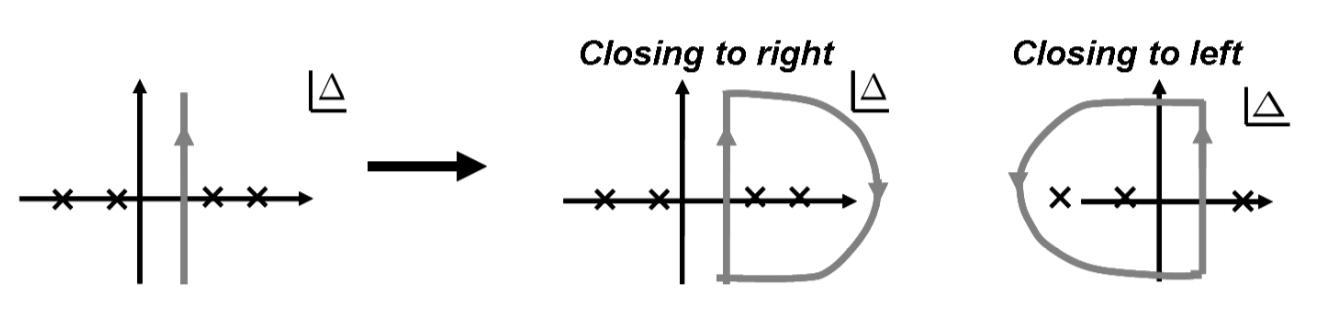
Figure 3: Left: The original integration contour of the principle series representation. One can close the contour either to the left or to the right, depending on the behaviour of the integrand at $|\Delta|\to\infty$. The integrand has poles on the real $\Delta$ axis.

From now on until subsection 3.4 we consider the case of equal external scaling dimensions: $a=b=0$. We close the integration contour in the $\Delta$ plane with a semi-circle at $|\Delta|\to\infty$, fig. 3. The integrand of eq. (32) has the following asymptotic behaviour as $|\Delta|\to\infty$:

$$\kappa_{J+\Delta}k_{\Delta-J}(z)k_{\Delta+J}({\bar{z}})k_{J-\Delta+2}(w)k_{\Delta+J}({\bar{w}})\to\frac{16}{\pi}\frac{\rho_{w}^{1+\frac{J}{2}}{\bar{\rho}_{w}}^{\frac{J}{2}}\rho_{z}^{-\frac{J}{2}}{\bar{\rho}_{z}}^{\frac{J}{2}}(\rho_{z}{\bar{\rho}_{z}}\rho_{w}^{-1}{\bar{\rho}_{w}})^{\frac{\Delta}{2}}}{\sqrt{(1-\rho_{w}^{2})(1-{\bar{\rho}_{w}}^{2})(1-\rho_{z}^{2})(1-{\bar{\rho}_{z}}^{2})}}.$$ (33)

From this we see that when the cross-ratios are such that $\rho_{z}{\bar{\rho}_{z}}\rho_{w}^{-1}{\bar{\rho}_{w}}=1$, the $\Delta$ integral is divergent and the kernel will have a contact term proportional to a delta function. We compute this contact term in the next subsection. Otherwise, the magnitude of $\rho_{z}{\bar{\rho}_{z}}\rho_{w}^{-1}{\bar{\rho}_{w}}$ determines whether we close the $\Delta$-contour to the left or to the right. Thus we expect our kernel to contain a step function as well, ie. both “bulk term” and “contact terms” as in eq. (3), which we reproduce for convenience:

$$K(z,{\bar{z}},w,{\bar{w}})=K_{B}\theta(\rho_{z}{\bar{\rho}_{z}}{\bar{\rho}_{w}}-\rho_{w})+K_{C}\frac{d\rho_{w}}{dw}\delta(\rho_{w}-\rho_{z}{\bar{\rho}_{z}}{\bar{\rho}_{w}})+K_{\emptyset}\theta(\rho_{w}-\rho_{z}{\bar{\rho}_{z}}{\bar{\rho}_{w}}).$$ (34)

The notation $K_{\emptyset}$ anticipates that the third term vanishes.

3.1.1 The Contact term $K_{C}$

Performing the $\Delta$ integral using the asymptotics in eq. (33) gives a delta function:

$$\frac{1}{4\pi i}\int_{1-i\infty}^{1+i\infty}d\Delta(\rho_{w}^{-1}\rho_{z}{\bar{\rho}_{z}}{\bar{\rho}_{w}})^{\frac{\Delta}{2}}=\delta(\rho_{w}^{-1}\rho_{z}{\bar{\rho}_{z}}{\bar{\rho}_{w}}-1).$$ (35)

The $J$ sum from eqs. (32) and (33) is then simply a geometric sum:

$$\ \widetilde{\sum_{J}}\rho_{w}^{1+\frac{J}{2}}{\bar{\rho}_{w}}^{\frac{J}{2}}\rho_{z}^{-\frac{J}{2}}{\bar{\rho}_{z}}^{\frac{J}{2}}+(z{\leftrightarrow}{\bar{z}})=\rho_{z}{\bar{\rho}_{z}}{\bar{\rho}_{w}}\frac{1-\rho_{z}{\bar{\rho}_{z}}{\bar{\rho}_{w}}^{2}}{(1-\rho_{z}{\bar{\rho}_{w}})(1-{\bar{\rho}_{z}}{\bar{\rho}_{w}})}$$ (36)

where we have used the constraint from the $\delta$-function to eliminate $\rho_{w}$ from the result. Combining eqs. (32)-(36) gives the result for the contact term of the kernel:

$$K\supset\frac{16}{\pi}\frac{1}{(w{\bar{w}})^{2}}\frac{\rho_{w}^{2}\delta(\rho_{w}-\rho_{z}{\bar{\rho}_{z}}{\bar{\rho}_{w}})}{\sqrt{(1-\rho_{w}^{2})(1-{\bar{\rho}_{w}}^{2})(1-\rho_{z}^{2})(1-{\bar{\rho}_{z}}^{2})}}\frac{1-\rho_{z}{\bar{\rho}_{z}}{\bar{\rho}_{w}}^{2}}{(1-\rho_{z}{\bar{\rho}_{w}})(1-{\bar{\rho}_{z}}{\bar{\rho}_{w}})}.$$ (37)

Dividing by the $\delta$-function and Jacobian $\frac{d\rho_{w}}{dw}$ included in eq. (34), this gives the formula recorded in the introduction, namely:

$$K_{C}(z,{\bar{z}},{\bar{w}})=\frac{4}{\pi}\frac{1}{{\bar{w}}^{2}}\left(\frac{1-\rho_{z}^{2}{\bar{\rho}_{z}}^{2}{\bar{\rho}_{w}}^{2}}{(1-\rho_{z}^{2})(1-{\bar{\rho}_{z}}^{2})(1-{\bar{\rho}_{w}}^{2})}\right)^{1/2}\frac{1-\rho_{z}{\bar{\rho}_{z}}{\bar{\rho}_{w}}^{2}}{(1-\rho_{z}{\bar{\rho}_{w}})(1-{\bar{\rho}_{z}}{\bar{\rho}_{w}})}.$$ (38)

The notation choice (34), with the Jacobian factored out, allows to directly integrate out $w$, leaving a single integral over ${\bar{w}}$:

$$\mathcal{G}^{t}(z,{\bar{z}})\Big{|}_{\rm contact}=\int_{0}^{1}d{\bar{w}}\ K_{C}(z,{\bar{z}},{\bar{w}})\ {\rm dDisc}[G(w,{\bar{w}})]\Big{|}_{\rho_{w}=\rho_{z}{\bar{\rho}_{z}}{\bar{\rho}_{w}}}\ .$$ (39)

3.1.2 The Bulk term $K_{B}$

We now move on to compute the kernel when $\rho_{z}{\bar{\rho}_{z}}\rho_{w}^{-1}{\bar{\rho}_{w}}\neq 1$. From eq. (33) we see that when the cross-ratios are in the regime $\rho_{z}{\bar{\rho}_{z}}\rho_{w}^{-1}{\bar{\rho}_{w}}>1$, we can close the contour to the left (ie. ${\rm Re}(\Delta)<1$), and the contribution from the arc at infinity will give zero. Likewise, when $\rho_{z}{\bar{\rho}_{z}}\rho_{w}^{-1}{\bar{\rho}_{w}}<1$ we close the contour to the right (ie. ${\rm Re}(\Delta)>1$) in order to drop the contribution from the arc at infinity, fig. 3.

Now we use the residue theorem to compute the $\Delta$ integral as a sum over residues of all the poles of the integrand of eq. (32). Each one of the four hypergeometric functions $k$’s has a tower of poles, and also $\kappa_{\beta}$ has a tower of poles. Performing the residue analysis, we find a few remarkable cancelations which significantly simplify the analysis. The first major simplification is that the poles of the conformal blocks always cancel in pairs after summing over $J$, and thus they give a zero contribution. This is the same mechanism as underlies the cancellation of spurious poles in the harmonic decomposition (20), see Caron-Huot:2017vep ; Simmons-Duffin:2017nub ; Gromov:2018hut . Furthermore, $\kappa_{\Delta+J}$ does not have any poles on the right (see eq. (24) with $a=b=0$), thus all the poles cancel. The kernel is identically zero in this region!

$$K(z,{\bar{z}},w,{\bar{w}})=0\qquad\text{for}\qquad\rho_{w}>\rho_{z}{\bar{\rho}_{z}}{\bar{\rho}_{w}}.$$ (40)

In other words the kernel is proportional to a unit step function $K(z,{\bar{z}},w,{\bar{w}})\propto\theta(\rho_{z}{\bar{\rho}_{z}}\rho_{w}^{-1}{\bar{\rho}_{w}}-1)$. This was expected physically, since the Lorentzian inversion formula is known to commute with the lightcone expansion: the step function ensures that the $z\to 0$ limit of the correlator is determined by the $w\to 0$ limit of the dDisc.

In the kinematics in which we close to the left, the kernel is non-zero. Again the spurious poles of the conformal blocks cancel out, but now there is a tower of double poles coming from $\kappa_{\Delta+J}$. These can be exhibited from the definition:

$$\kappa_{\beta}\equiv\frac{1}{2\pi^{2}}\frac{\Gamma^{4}(\frac{\beta}{2})}{\Gamma(\beta)\Gamma(\beta-1)}=-\frac{\cot^{2}(\frac{\pi\beta}{2})}{\pi^{2}}\frac{1}{\kappa_{2-\beta}}.$$ (41)

Since $\beta=\Delta+J$, we can label the poles by a positive integer $m$:

$$\Delta_{\rm pole}=-J-2m,\ \ \text{with}\ \ \ m=0,1,2,\ldots\infty.$$ (42)

Thus from eqs. (32), (41), and the residue theorem, we have:

$$K_{B}=\frac{2}{\pi^{2}}\frac{1}{w^{2}{\bar{w}}^{2}}\ \widetilde{\sum_{J}}\sum_{m=0}^{\infty}\frac{d}{dm^{\prime}}\bigg{(}\frac{k_{-2J-2m^{\prime}}(z)k_{-2m^{\prime}}({\bar{z}})k_{2J+2m^{\prime}+2}(w)k_{-2m^{\prime}}({\bar{w}})}{2\pi^{2}\kappa_{2m^{\prime}+2}}\bigg{)}\Bigg{|}_{m^{\prime}=m}+(z{\leftrightarrow}{\bar{z}}),$$ (43)

where we took the derivative with respect to $m^{\prime}$ (as required by the residue theorem for the case of double poles), and then plugged the integer value $m$. Now we notice that $J$ appears in only two hypergeometric functions; in fact the $J$-sum is telescopic and can be computed exactly, see eq. (114). Performing the $J$-sum first we thus obtain

$$K_{B}=\frac{4}{\pi^{2}}\frac{1}{w^{2}{\bar{w}}^{2}}\mathcal{D}_{2}\sum_{m=0}^{\infty}\frac{d}{dm^{\prime}}\bigg{(}\frac{\Gamma^{2}(2m^{\prime}+1)}{2\Gamma^{4}(m^{\prime}+1)}k_{-2m^{\prime}}(z)k_{-2m^{\prime}}({\bar{z}})k_{-2m^{\prime}}({\bar{w}})k_{2m^{\prime}+2}(w)\bigg{)}\Bigg{|}_{m^{\prime}=m}\,,$$ (44)

where $\mathcal{D}_{2}$ is a first-order differential operator acting on $z,{\bar{z}}$ and $w$ and defined in eq. (113). To summarize, the dispersion kernel $K$ defined by eq. (29) is now written explicitly in the form (34) with the contact term (38) plus the bulk part (44), the latter still to be simplified. It remains to perform the sum $m$ over the tower of poles. This sum seems formidable: the summand is a derivative $\frac{d}{dm^{\prime}}$ of a product of 4 hypergeometric functions. Amazingly, it can be performed exactly!

3.2 Main result from Legendre PPPQ sum

We will now perform the sum in eq. (44), namely:

$$S\equiv\sum_{m=0}^{\infty}\frac{d}{dm^{\prime}}\bigg{(}\frac{\Gamma^{2}(2m^{\prime}+1)}{2\Gamma^{4}(m^{\prime}+1)}k_{-2m^{\prime}}(z)k_{-2m^{\prime}}({\bar{z}})k_{-2m^{\prime}}({\bar{w}})k_{2m^{\prime}+2}(w)\bigg{)}\Bigg{|}_{m^{\prime}=m}.$$ (45)

To get some intuition, we first notice that, near ${\bar{w}}\to 1$, each term has at most a logarithmic singularity. This is because $k_{-2m^{\prime}}({\bar{w}})$ is polynomial for integer $m^{\prime}$; a singularity can only appear when the $\frac{d}{dm^{\prime}}$ derivative acts on $k_{-2m^{\prime}}({\bar{w}})$,

$$\frac{dk_{-2m^{\prime}}({\bar{w}})}{dm^{\prime}}\Big{|}_{m^{\prime}=m}=\frac{\Gamma^{2}(m+1)}{\Gamma(2m+1)}P_{m}(\hat{{\bar{w}}})\times\tfrac{1}{2}\log(1-{\bar{w}})+\text{(non-singular)}$$ (46)

where for conciseness in this section we use a hat notation in which $\hat{w}\equiv\frac{2}{w}-1$. Let us first focus on the coefficient of the $\log$ term, that is the discontinuity around ${\bar{w}}=1$.

We also notice that plugging $m^{\prime}=m=\text{integer}$, the hypergeometric functions reduce to Legendre functions:

$$k_{-2m}(z)=\frac{\Gamma^{2}(m+1)}{\Gamma(2m+1)}P_{m}(\hat{z}),\qquad k_{\beta}(z)=2\frac{\Gamma(\beta)}{\Gamma^{2}(\frac{\beta}{2})}Q_{\frac{\beta}{2}-1}(\hat{z}).$$ (47)

where $P_{m}(\hat{z})$ and $Q_{m}(\hat{z})$ are Legendre polynomials and Legendre functions of the second kind, respectively. Thus the log part of the sum becomes:

$$S\Big{|}_{\frac{1}{2}\log(1-{\bar{w}})}=\sum_{m=0}^{\infty}(2m+1)P_{m}(\hat{z})P_{m}(\hat{{\bar{z}}})P_{m}(\hat{{\bar{w}}})Q_{m}(\hat{w}).$$ (48)

So we must now compute this $(2m+1)P_{m}P_{m}P_{m}Q_{m}$ sum. Luckily, the coefficient $(2m+1)$ in the sum is the canonical coefficient which often appears with Legendre functions! Encouragingly, we further notice that a similar sum appeared for the scattering amplitude dispersion relation in eq. (14), involving $(2m+1)P_{m}Q_{m}$—which can be realized in the limit ${\bar{z}},{\bar{w}}\to 1$ of the current one.

It turns out that such sums (with precisely the coefficient $(2m+1)$) have been evaluated in the mathematics literature, dating back to Watson who computed a PPP sum Watson . Specifically, we use the result in eqs. (3.8)-(3.10) of baranov1 , who computed the $PPPP$ sum. To uplift his result to our $PPPQ$ sum in eq. (48), we need simply replace the $P_{J}(\hat{w})$ with a $Q_{J}(\hat{w})$, which can be done using the single-variable dispersion relation in the footnote below eq. (2.1.1). In fact this step is completely trivial: the PPPP sum given in baranov1 is defined in the interval $\hat{{\bar{w}}}\in[-1,1]$, and has square-root branch points at the boundary. The function whose discontinuity is this, has exactly the same functional form, but now viewed as a function of the complex plane minus the interval. The result of the sum is thus (see also Hearingen ; Rahman ):

$$S\Big{|}_{\frac{1}{2}\log(1-{\bar{w}})}=\frac{4\rho_{w}{\bar{\rho}_{w}}\rho_{z}{\bar{\rho}_{z}}\textbf{K}(x)}{\pi\sqrt{({\bar{\rho}_{w}}\rho_{z}-\rho_{w}{\bar{\rho}_{z}})({\bar{\rho}_{w}}{\bar{\rho}_{z}}-\rho_{w}\rho_{z})(\rho_{z}{\bar{\rho}_{z}}-\rho_{w}{\bar{\rho}_{w}})(1-\rho_{w}{\bar{\rho}_{w}}\rho_{z}{\bar{\rho}_{z}})}}\ ,$$ (49)

where $\textbf{K}(x)$ is the elliptic integral of the first kind:

$$\textbf{K}(x)\equiv\int_{0}^{\frac{\pi}{2}}\frac{d\theta}{\sqrt{1-x\sin^{2}\theta}}=\tfrac{\pi}{2}\ {}_{2}F_{1}(\tfrac{1}{2},\tfrac{1}{2},1,x),$$ (50)

and $x$ is the following combination of $\rho$’s, recorded previously in eq. (5):

$$x\equiv\frac{\rho_{z}{\bar{\rho}_{z}}\rho_{w}{\bar{\rho}_{w}}(1-\rho_{z}^{2})(1-{\bar{\rho}_{z}}^{2})(1-\rho_{w}^{2})(1-{\bar{\rho}_{w}}^{2})}{({\bar{\rho}_{w}}\rho_{z}-\rho_{w}{\bar{\rho}_{z}})({\bar{\rho}_{w}}{\bar{\rho}_{z}}-\rho_{w}\rho_{z})(\rho_{z}{\bar{\rho}_{z}}-\rho_{w}{\bar{\rho}_{w}})(1-\rho_{w}{\bar{\rho}_{w}}\rho_{z}{\bar{\rho}_{z}})}.$$ (51)

We are not quite done yet—recalling eq. (45), we need to account for the derivative $d/dm^{\prime}$, or, equivalently, we need to find the function whose $\log$ term is eq. (49). This appears to be a difficult task, and so we try instead to make an educated guess. As boundary data, one can directly show that eq. (45) should be regular at $\rho_{w}\to\rho_{z}{\bar{\rho}_{z}}\rho_{\bar{w}}$, corresponding to $x\to 1$. The $\frac{1}{2}\log(1-{\bar{w}})$ term we have found corresponds to $\log x$ as $x\to 0$. Our guess is to look for a second solution to the same hypergeometric differential equation, but satisfying these other boundary conditions. In fact there is a unique candidate, which turns out to be also an elliptic function:

$${-}\pi\textbf{K}(1-x)=\textbf{K}(x)\log(x)+\text{non-singular}.$$ (52)

This equation states that the coefficient of the log singular terms of an elliptic function is itself an elliptic function, with a changed argument. Our educated guess, extending eq. (49), is thus:

$$S=\frac{-4\rho_{w}{\bar{\rho}_{w}}\rho_{z}{\bar{\rho}_{z}}\textbf{K}(1-x)}{\sqrt{({\bar{\rho}_{w}}\rho_{z}-\rho_{w}{\bar{\rho}_{z}})({\bar{\rho}_{w}}{\bar{\rho}_{z}}-\rho_{w}\rho_{z})(\rho_{z}{\bar{\rho}_{z}}-\rho_{w}{\bar{\rho}_{w}})(1-\rho_{w}{\bar{\rho}_{w}}\rho_{z}{\bar{\rho}_{z}})}}\ .$$ (53)

A numerical evaluation of eq. (45), or its series expansion at small ${\bar{w}}$, both confirm that this ansatz is correct!

We are now done; the bulk term in the kernel is obtained as $K_{B}=\frac{4}{\pi^{2}}\frac{1}{w^{2}{\bar{w}}^{2}}\mathcal{D}_{2}S$, from eq. (44). Performing some simplifications, this gives us the form recorded in eq. (4), namely:

$$K_{B}(z,{\bar{z}},w,{\bar{w}})=-\frac{1}{64\pi}\left(\frac{z{\bar{z}}}{w{\bar{w}}}\right)^{\frac{3}{2}}\frac{({\bar{w}}-w)(\frac{1}{z}+\frac{1}{{\bar{z}}}+\frac{1}{w}+\frac{1}{{\bar{w}}}-2)}{\big{(}(1-z)(1-{\bar{z}})(1-w)(1-{\bar{w}})\big{)}^{\frac{3}{4}}}\ x^{\frac{3}{2}}{}_{2}F_{1}(\tfrac{1}{2},\tfrac{3}{2},2,1-x).$$ (55)

An equivalent expression, suitable for integrating with respect to $\rho$-variables, is:

$$K_{B}(z,{\bar{z}},w,{\bar{w}})dwd{\bar{w}} =-\frac{1}{\pi}\frac{d\rho_{w}d{\bar{\rho}_{w}}}{(\rho_{w}{\bar{\rho}_{w}})^{3/2}}\left(\frac{\rho_{z}{\bar{\rho}_{z}}}{(1-\rho_{z}^{2})(1-{\bar{\rho}_{z}}^{2})}\right)^{3/2}\left(\frac{1}{z}+\frac{1}{{\bar{z}}}+\frac{1}{w}+\frac{1}{{\bar{w}}}-2\right)$$ (56)

$$\qquad\times\frac{(\rho_{w}-{\bar{\rho}_{w}})(1-\rho_{w}{\bar{\rho}_{w}})}{\sqrt{(1-\rho_{w}^{2})(1-{\bar{\rho}_{w}}^{2})}}x^{\frac{3}{2}}{}_{2}F_{1}(\tfrac{1}{2},\tfrac{3}{2},2,1-x).$$

3.3 Match with $d=4$ and differential equation

We will now similarly derive the dispersion relation in $d=4$ spacetime dimension and show that it equals the one in $d=2$, due to interesting identities. Since the steps are very similar, we omit details and emphasize the few changes. The conformal blocks in $d=4$ are given by:

$$G_{J,\Delta}(z,{\bar{z}})=\frac{z{\bar{z}}}{{\bar{z}}-z}\Big{(}k_{\Delta-J-2}(z)k_{\Delta+J}({\bar{z}})-k_{\Delta+J}(z)k_{\Delta-J-2}({\bar{z}})\Big{)}.$$ (57)

The extra prefactor, different measure, and shift in the argument of $k$ functions (to $\Delta-J-2$) lead to mild changes in eq. (32):

$$\begin{aligned} &K^{(d=4)}=\frac{1}{4\pi i}\frac{z{\bar{z}}}{z-{\bar{z}}}\frac{{\bar{w}}-w}{w^{3}{\bar{w}}^{3}}\\ &\times\sum_{J=0}^{\infty}\int_{2-i\infty}^{2+i\infty}d\Delta\ \kappa_{J+\Delta}k_{\Delta-J-2}(z)k_{\Delta+J}({\bar{z}})k_{J-\Delta+4}(w)k_{\Delta+J}({\bar{w}})\ +\ (z\leftrightarrow{\bar{z}}).\end{aligned}$$ (58)

As in the $d=2$ case, we close the contour in the $\Delta$ plane and pick up the residues of the poles, being careful with the behavior at infinity which gives rise to contact terms.

3.3.1 Contact term

We first compare the contact terms, which originate from the large-$\Delta$ asymptotics given in eq. (33). Following the steps leading to eq. (36) we find that the kernels match due to the following identity:

$$\rho_{w}\frac{{\bar{w}}-w}{w{\bar{w}}}\frac{z{\bar{z}}}{z-{\bar{z}}}\sum^{\infty}_{J=0}\bigg{(}\rho_{z}^{-1}(\rho_{w}{\bar{\rho}_{w}}\rho_{z}^{-1}{\bar{\rho}_{z}})^{\frac{J}{2}}-{\bar{\rho}_{z}}^{-1}(\rho_{w}{\bar{\rho}_{w}}{\bar{\rho}_{z}}^{-1}\rho_{z})^{\frac{J}{2}}\bigg{)}\Big{|}_{\rho_{w}={\bar{\rho}_{w}}\rho_{z}{\bar{\rho}_{z}}}$$

$$=\widetilde{\sum}^{\infty}_{J=0}\bigg{(}(\rho_{w}{\bar{\rho}_{w}}\rho_{z}^{-1}{\bar{\rho}_{z}})^{\frac{J}{2}}+(\rho_{w}{\bar{\rho}_{w}}{\bar{\rho}_{z}}^{-1}\rho_{z})^{\frac{J}{2}}\bigg{)}\Big{|}_{\rho_{w}={\bar{\rho}_{w}}\rho_{z}{\bar{\rho}_{z}}}$$ (59)

which is rather surprising but can be verified by explicit computation on both sides. We thus find that the contact term in $d=4$ matches that of $d=2$:

$$K^{(d=2)}_{C}({\bar{\rho}_{w}},\rho_{z},{\bar{\rho}_{z}})=K^{(d=4)}_{C}({\bar{\rho}_{w}},\rho_{z},{\bar{\rho}_{z}}).$$ (60)

3.3.2 Bulk term

The agreement for the bulk term will be rather more remarkable. Again we find that spurious poles from the blocks cancel out pairwise, so we only need to keep the poles from $\kappa$ in eq. (LABEL:d=4_sum), which are in the left-hand $\Delta$-plane. The summation over $J$ can be performed similarly to eq. (44), and leads to a different operator acting on the same sum $S$ defined in eq. (45):

$$K_{B}^{(d=4)}=\frac{4}{\pi^{2}}\frac{1}{w^{2}{\bar{w}}^{2}}\mathcal{D}_{4}S$$ (61)

with

$$\mathcal{D}_{4}\equiv\frac{z{\bar{z}}}{z-{\bar{z}}}\frac{w-{\bar{w}}}{w{\bar{w}}}\Big{(}\Big{(}\frac{zw(1-w)}{z-w}-\frac{{\bar{z}}w(1-w)}{{\bar{z}}-w}\Big{)}\partial_{w}-\frac{zw(1-z)}{z-w}\partial_{z}+\frac{{\bar{z}}w(1-{\bar{z}})}{{\bar{z}}-w}\partial_{{\bar{z}}}\Big{)},$$ (62)

instead of $\mathcal{D}_{2}$ given in eq. (113). Remarkably, however, it is possible to verify using the explicit form of $S$ in eq. (53) that the two kernels agree:

$$\Big{(}\mathcal{D}_{4}-\mathcal{D}_{2}\Big{)}S=0.$$ (63)

As a result, the 4d bulk kernel is equal to the 2d one!

$$K^{(d=4)}_{B}(z,{\bar{z}},w,{\bar{w}})=K^{(d=2)}_{B}(z,{\bar{z}},w,{\bar{w}}).$$ (64)

In summary, we showed that the dispersion relation is the same in $d=4$ and $d=2$. This strengthens our intuition that the dispersion relation should not depend on the space-time dimension $d$; it would be interesting to show this in other dimensions.

The agreement between the $d=2$ and $d=4$ kernels gives us an interesting first-order differential equation satisfied by the $PPPQ$ sum $S$. Turning the logic around, we can now use this differential equation to help determine the kernel in the general case of unequal scaling dimensions.

3.4 Differential equation for unequal scaling dimensions

We turn to the case of a generic 4-point correlator $\langle\mathcal{O}_{1}\ldots\mathcal{O}_{4}\rangle$ of scalars with unequal scaling dimension: $a=\frac{1}{2}(\Delta_{2}-\Delta_{1})\neq 0$ and $b=\frac{1}{2}(\Delta_{3}-\Delta_{4})\neq 0$. We will be brief and emphasize the main points. There is formally no change to eq. (32), namely:

$$K^{(a,b)}=\frac{\mu(w,{\bar{w}})^{(a,b)}}{4\pi i}\ \ \widetilde{\sum_{J}}\int_{1-i\infty}^{1+i\infty}d\Delta\ \kappa_{J+\Delta}^{(a,b)}k_{\Delta-J}^{(a,b)}(z)k_{\Delta+J}^{(a,b)}({\bar{z}})k_{J-\Delta+2}^{(a,b)}(w)k_{\Delta+J}^{(a,b)}({\bar{w}})+(z{\leftrightarrow}{\bar{z}}),$$ (65)

where we have simply made explicit the dependence on $a$ and $b$ of the various factors. One may easily derive the contact term, by making a simple replacement in eq. (38):

$$K_{C}^{(a,b)}(z,{\bar{z}},w,{\bar{w}})=\left(\frac{(1-w)(1-{\bar{w}})}{(1-z)(1-{\bar{z}})}\right)^{\frac{a+b}{2}}K_{C}^{(0,0)}(z,{\bar{z}},w,{\bar{w}}).$$ (66)

The bulk term comes from poles of $\kappa_{\Delta+J}$, since spurious poles from the conformal blocks cancel in pairs just as in the $a=b=0$ case. As opposed to that case, however, the poles of $\kappa_{\Delta+J}$ are now single poles instead of double poles. After performing the $J$ sum using the identity in eq. (112), we find the generalization of eq. (44):

$$K_{B}^{(a,b)}(z,{\bar{z}},w,{\bar{w}})=\mu^{(a,b)}(w,{\bar{w}})\ \mathcal{D}_{2}\Big{(}S^{(a,b)}_{a}+S^{(a,b)}_{-a}+S^{(b,a)}_{b}+S^{(b,a)}_{-b}\Big{)}$$ (67)

where $\mathcal{D}_{2}$, given in eq. (113), is the same differential operator as before, and we have defined:

$$S_{a^{\prime}}^{(a,b)}\equiv\sum_{m=0}^{\infty}\frac{\sin(2\pi a^{\prime})}{2\pi\ m!}\frac{\Gamma^{2}_{1+2a^{\prime}+2m}k_{-2m-2a^{\prime}}^{(a,b)}(z)k_{-2m-2a^{\prime}}^{(a,b)}({\bar{z}})k_{-2m-2a^{\prime}}^{(a,b)}({\bar{w}})k_{2m+2+2a^{\prime}}^{(a,b)}(w)}{\Gamma_{1+2a^{\prime}+m}\Gamma_{1+a^{\prime}-b+m}\Gamma_{1+a^{\prime}+b+m}\sin(\pi(a-b))\sin(\pi(a+b))}$$ (68)

using the notation $\Gamma_{x}\equiv\Gamma(x)$. The sum in eq. (68) contains products of four hypergeometric functions which cannot be reduced to Legendre functions. Thus it may seem hopeless to try to compute it directly. However, we may say a lot about the result using differential equations.

A key observation is that dimension-independence still holds, that is:

$$(\mathcal{D}_{2}-\mathcal{D}_{4})S^{(a,b)}_{a^{\prime}}=0.$$ (69)

We could prove this using hypergeometric identities to rewrite the derivatives as shift on the index $m$ of the $k$ functions, and showing that $m$ sum becomes telescopic; it may also be readily verified order by order in $w$. Notice that both $\mathcal{D}_{2}$ and $\mathcal{D}_{4}$ are first-order differential operators (and independent of $a$ and $b$). In fact, thanks to the manifest permutation symmetry of $S^{(a,b)}_{a^{\prime}}$ in $(z,{\bar{z}},{\bar{w}})$, this identity and its permutations give two linearly independent differential equations. The fact that a function is annihilated by two first-order equations implies that it factors through the two variables which represent its zero-modes, up to an overall factor:

$$S_{a^{\prime}}^{(a,b)}=\frac{\sqrt{z\bar{z}w\bar{w}}}{y^{1/2+a+b}}\times\tilde{S}_{a^{\prime}}^{(a,b)}(x,y)$$ (70)

where $x$ is in eq. (5), reproduced here for convenience, and $y$ is:

$$x =\frac{\rho_{z}{\bar{\rho}_{z}}\rho_{w}{\bar{\rho}_{w}}(1-\rho_{z}^{2})(1-{\bar{\rho}_{z}}^{2})(1-\rho_{w}^{2})(1-{\bar{\rho}_{w}}^{2})}{({\bar{\rho}_{w}}{\bar{\rho}_{z}}-\rho_{w}\rho_{z})({\bar{\rho}_{w}}\rho_{z}-\rho_{w}{\bar{\rho}_{z}})({\bar{\rho}_{z}}\rho_{z}-{\bar{\rho}_{w}}\rho_{w})(1-\rho_{w}\rho_{z}{\bar{\rho}_{w}}{\bar{\rho}_{z}})}\ ,$$ (71)

$$y =\frac{(1-\rho_{z})(1-\rho_{{\bar{z}}})(1-\rho_{w})(1-\rho_{{\bar{w}}})}{(1+\rho_{z})(1+\rho_{{\bar{z}}})(1+\rho_{w})(1+\rho_{{\bar{w}}})}=\sqrt{(1-z)(1-{\bar{z}})(1-w)(1-{\bar{w}})}\ .$$ (72)

The sums $\tilde{S}^{(a,b)}_{a^{\prime}}$ are further constrained by second-order differential equations, which encode that the SL(2,R) Casimir eigenvalue with respect to each of the four variable are the same as can be seen from eq. (68). From these we find two equations on $\tilde{S}$:

$$0 =\left[x^{2}(1-x)\partial_{x}^{2}-x^{2}\partial_{x}+y^{2}\partial_{y}^{2}+y\partial_{y}-\tfrac{1}{2}x^{2}(1-y^{2})\partial_{x}\partial_{y}+(\tfrac{1}{4}-a^{2}-b^{2})\right]\tilde{S}^{(a,b)}_{a^{\prime}},$$ (73)

$$0 =\left[(x^{2}(1-y)^{2}+4xy)\partial_{x}\partial_{y}-2y\partial_{y}-4ab\right]\tilde{S}^{(a,b)}_{a^{\prime}}.$$

These two, together with the boundary condition that $S_{a^{\prime}}^{(a,b)}(x,y)\propto x^{1/2+a^{\prime}}(1+O(x))$ as $x\to 0$, with a constant easily determined from the $m=0$ term in eq. (68), completely determine the functions $S$.

Before discussing solutions, let us make an observation about the $a=b=0$ case: the second equation can be used to fix the $y$ dependence of each term recursively in a series in $x$; when $ab=0$, it implies that the solution is independent of $y$: $\partial_{y}\tilde{S}^{(a,b)}_{a^{\prime}}=0$. The first equation then reduces to that satisfied by the elliptic function $\sqrt{x}{\bf K}(1-x)$. With this method it is thus straightforward to derive the result (53) which we previously only guessed. The key is the identity in eq. (69), which states that the kernels in $d=2$ and $d=4$ are the same and which leads to eq. (70).

Instead of looking at the individual sums $\tilde{S}_{a^{\prime}}^{(a,b)}$ we now focus on the specific combination in eq. (67) and the actual kernel. It is convenient to explicitly act with the differential operator $\mathcal{D}_{2}$ on the prefactor in eq. (70). In a convenient normalization the kernel is then

$$K_{B}^{(a,b)}=-\frac{1}{64\pi}\left(\frac{z{\bar{z}}}{w{\bar{w}}}\right)^{\frac{3}{2}}\frac{({\bar{w}}-w)(\frac{1}{z}+\frac{1}{{\bar{z}}}+\frac{1}{w}+\frac{1}{{\bar{w}}}-2)}{y^{3/2+a+b}}\ \tilde{K}_{B}^{(a,b)}(x,y)$$ (74)

where

$$\tilde{K}_{B}^{(a,b)}(x,y)\equiv-8\pi x^{2}\partial_{x}\Big{(}\tilde{S}^{(a,b)}_{a}+\tilde{S}^{(a,b)}_{-a}+\tilde{S}^{(b,a)}_{b}+\tilde{S}^{(b,a)}_{-b}\Big{)}.$$ (75)

From eqs. (73) we derive differential equations satisfied by $\tilde{K}$:

$$0 =\left[x^{2}(1-x)\partial_{x}^{2}-2x\partial_{x}+y^{2}\partial_{y}^{2}+y\partial_{y}-\tfrac{1}{2}x^{2}(1-y^{2})\partial_{x}\partial_{y}+(\tfrac{9}{4}-a^{2}-b^{2})\right]\tilde{K}_{B}^{(a,b)}(x,y),$$ (76)

$$0 =\left[(x^{2}(1-y)^{2}+4xy)\partial_{x}\partial_{y}-6y\partial_{y}-4ab\right]\tilde{K}_{B}^{(a,b)}(x,y).$$

These conditions ensure that the dispersion relation commutes with the $s$-channel quadratic Casimir. While we have not been able to solve these in closed form, we can state the following results:

• The kernel $\tilde{K}_{B}^{(a,b)}(x,y)$ is regular around $x=1$. While this is not true for the individual sums in eq. (68) (each has a logarithmic singularity), this is a special property of the combination in eq. (67). The kernel is then the unique regular solution to (74) with the boundary condition

  $$\lim_{x\to 1}\tilde{K}_{B}^{(a,b)}(x,y)=1-4(a+b)^{2}+16ab\frac{y}{y+1}.$$ (77)

  (We could get the constant by combining the eqs. (76) into a single fourth-order one with no $y$-derivatives, and solving it along the $y=1$ line in terms of ${}_{4}F_{3}$ hypergeometric functions.)

• The limits as $y\to 0$ and $y\to\infty$ are regular, and equal to a simply generalization of eq. (38):

  $$\lim_{y\to 0}\tilde{K}_{B}^{(a,b)}(x,y) =(1-4(a+b)^{2})x^{3/2+a+b}{}_{2}F_{1}(\tfrac{1}{2}+a+b,\tfrac{3}{2}+a+b,2,1-x),$$ (78)

  $$\lim_{y\to\infty}\tilde{K}_{B}^{(a,b)}(x,y) =(1-4(a-b)^{2})x^{3/2+a-b}{}_{2}F_{1}(\tfrac{1}{2}+a-b,\tfrac{3}{2}+a-b,2,1-x).$$

• A Taylor series in $(1-x)$ can be obtained using just the second of eqs. (76), together with the previous limits; each term is polynomial in $\frac{y}{1+y}$.

In summary, for unequal scalar operators, the kernel takes the form in eq. (1), with the contact term given explicitly in eq. (66), and bulk term in eq. (74) implicitly described by the above.

Let us briefly comment on the special case: $a=0$ and $b=\frac{1}{2}$, where the bulk term $K_{B}$ identically vanishes. (This could be seen directly from the lack of poles of $\kappa$ in eq. (24).) This corresponds physically to a case where the double-discontinuity (26) is effectively a single discontinuity! Only the contact term (66) remains. We observe also that it is free of square roots (when written in terms of $\rho$’s). (More generally, when $a$ is integer and $b$ is half-integer, the contact kernel $\tilde{K}_{C}(z,{\bar{z}},{\bar{w}})$ does not contain square roots.) The dispersion relation then reduces to

$$\mathcal{G}^{t,(0,\frac{1}{2})}(z,{\bar{z}})=\frac{1}{\pi}\int_{0}^{1}\frac{d{\bar{\rho}_{w}}}{{\bar{\rho}_{w}}^{2}}\frac{1-\rho_{z}{\bar{\rho}_{z}}{\bar{\rho}_{w}}^{2}}{(1-\rho_{z}{\bar{\rho}_{w}})(1-{\bar{\rho}_{z}}{\bar{\rho}_{w}})}\frac{(1-\rho_{w})(1-{\bar{\rho}_{w}})}{(1-\rho_{z})(1-{\bar{\rho}_{z}})}{\rm dDisc}\big{[}\mathcal{G}(w,{\bar{w}})\big{]}_{\rho_{w}=\rho_{z}{\bar{\rho}_{z}}{\bar{\rho}_{w}}}.$$ (79)

Upon further inspection, this could be recognized as a single-variable dispersion relation of the form of section 2.1, taken with fixed value of the ratio ${\bar{\rho}_{w}}/\rho_{w}$ and acting on a certain rescaling of the correlator. This ratio more generally will play an important role in the next section.

4 Direct proof of dispersion relation

Having now obtained its kernel, we will now prove directly that the dispersion integral (1) indeed reconstructs correlators. This may be viewed as a theorem in complex analysis, independent of the CFT origin of the formula. This will show directly the validity of the formula in any dimension, and will enable us to go beyond the situations where the Lorentzian inversion formula converges.

We begin by observing that the contact term and bulk term of the kernel (see eqs. (34), (38) and (55)), are not independent, disparate entities. Rather, they combine into the discontinuity of a single “pre-kernel”:

$$K_{\rm pre}(z,{\bar{z}},w,{\bar{w}})=-\frac{1}{32}\frac{{\bar{w}}-w}{w{\bar{w}}}\frac{(z{\bar{z}}w{\bar{w}})^{\frac{3}{2}}(\frac{1}{z}+\frac{1}{{\bar{z}}}+\frac{1}{w}+\frac{1}{{\bar{w}}}-2)}{((1-w)(1-{\bar{w}})(1-z)(1-{\bar{z}}))^{\frac{3}{4}}}x^{\frac{3}{2}}\ _{2}F_{1}(\tfrac{1}{2},\tfrac{3}{2},1,x).$$ (80)

Near $x=1$, the hypergeometric function above satisfies:

$$\ _{2}F_{1}(\tfrac{1}{2},\tfrac{3}{2},1,x)=\frac{2}{\pi(1-x)}-\frac{1}{2\pi}\ {}_{2}F_{1}(\tfrac{1}{2},\tfrac{3}{2},2,1-x)\log(1-x)+\text{(non-singular)}.$$ (81)

Using that

$$1-x=\frac{(\rho_{z}-{\bar{\rho}_{z}}\rho_{w}{\bar{\rho}_{w}})({\bar{\rho}_{z}}-\rho_{z}\rho_{w}{\bar{\rho}_{w}})({\bar{\rho}_{w}}-\rho_{w}\rho_{z}{\bar{\rho}_{z}})(\rho_{z}{\bar{\rho}_{z}}{\bar{\rho}_{w}}-\rho_{w})}{({\bar{\rho}_{z}}{\bar{\rho}_{w}}-\rho_{w}\rho_{z})(\rho_{z}{\bar{\rho}_{w}}-\rho_{w}{\bar{\rho}_{z}})(\rho_{z}{\bar{\rho}_{z}}-\rho_{w}{\bar{\rho}_{w}})(1-\rho_{w}\rho_{z}{\bar{\rho}_{w}}{\bar{\rho}_{z}})},$$ (82)

we see that the pre-kernel has both a pole and branch cut at $\rho_{w}\to\rho_{z}{\bar{\rho}_{z}}{\bar{\rho}_{w}}$, whose residue and discontinuity precisely match, respectively, the contact term and bulk terms:

$$K_{C}={\rm Res}_{\rho_{w}=\rho_{z}{\bar{\rho}_{z}}{\bar{\rho}_{w}}}[K_{\rm pre}],\qquad K_{B}=\frac{1}{2\pi}{\rm Disc}_{\rho_{w}\to\rho_{z}{\bar{\rho}_{z}}{\bar{\rho}_{w}}}[K_{\rm pre}]\quad(\rho_{w}<\rho_{z}{\bar{\rho}_{z}}{\bar{\rho}_{w}}).$$ (83)

This enables to combine these terms into a single contour integral:

$$\boxed{\mathcal{G}^{t}(z,{\bar{z}})=\frac{1}{2\pi i}\int_{\mathcal{C}_{w}}dw\int_{0}^{1}d{\bar{w}}\ K_{\rm pre}(z,{\bar{z}},w,{\bar{w}})\ {\rm dDisc}[\mathcal{G}(w,{\bar{w}})]}$$ (84)

where $\mathcal{C}_{w}$ is a “keyhole” contour going from the origin to the origin counter-clockwise around its maximum $w_{\rm max}$ corresponding to $\rho_{w}=\rho_{z}{\bar{\rho}_{z}}{\bar{\rho}_{w}}$ (similar to the contour $\mathcal{C}_{\sigma}$ in fig.  4(a)). The existence of such a pre-kernel is very suggestive of a contour deformation argument leading to the dispersion relation.

4.1 Contour deformation trick

We will now describe a contour in two complex variables, which, fortunately for us, takes on a simple factorized form in suitable variables. The “good variables”, as suggested by the degenerate case in eq. (79), are the geometric mean and ratio of $\rho$-coordinates:

$$\sigma_{z}=\sqrt{\rho_{z}{\bar{\rho}_{z}}},\quad\eta_{z}=\sqrt{\rho_{z}/{\bar{\rho}_{z}}},\quad\sigma_{w}=\sqrt{\rho_{w}{\bar{\rho}_{w}}},\quad\eta_{w}=\sqrt{\rho_{w}/{\bar{\rho}_{w}}}.$$ (85)

Physically, in the Euclidean cylinder, $\sigma$ is a radial coordinate and $\eta=e^{i\theta}$ is an angular variable. The singularities which will be relevant for our argument are shown in fig. 4. The complete list of singularities of the kernel and pre-kernel come from where $x=0,1,\infty$, namely:

$$x =0: \eta_{w} \in\{\pm\sigma_{w},\pm\sigma_{w}^{-1}\}, \sigma_{w} \in\{0,\pm\eta_{w},\pm\eta_{w}^{-1},\infty\},$$ (86)

$$x =1: \eta_{w} \in\{\pm\sigma_{z},\pm\sigma_{z}^{-1}\}, \sigma_{w} \in\{\pm\eta_{z},\pm\eta_{z}^{-1}\},$$

$$x =\infty: \eta_{w} \in\{\pm\eta_{z},\pm\eta_{z}^{-1}\}, \sigma_{w} \in\{\pm\sigma_{z},\pm\sigma_{z}^{-1}\}.$$

Notice that each $\eta_{w}$-plane singularity is reflected four-fold: by $\eta\mapsto\eta^{-1}$, which is parity $w{\leftrightarrow}{\bar{w}}$, and by $\eta\mapsto-\eta$, which interchanges the $t$ and $u$ channels (ie. swaps operators $1$ and $2$ in the four-point correlator).

We will now see that the dispersion relation can be derived starting from the identity:

$$0=\oint_{\mathcal{C}_{\sigma}\times\{|\eta_{w}|=1\}}K_{\rm pre}(z,{\bar{z}},w,{\bar{w}})G(w,{\bar{w}})$$ (87)

where the original contour, shown in fig. 4, is a product of a keyhole in $\sigma_{w}$ (similar to eq. (84)), times the unit circle $\eta_{w}=1$, and then deforming the contour. This will hinge on several properties that the pre-kernel (80) (remarkably!) combines:

1. It is odd under $w{\leftrightarrow}{\bar{w}}$ due to the factor $(w-{\bar{w}})$.

2. The branch cut at $x=\infty$ is only logarithmic.

3. It has a simultaneous double pole when $(\sigma_{w},\eta_{w})=(\sigma_{z},\eta_{z})$, e.g. $\frac{1}{(\eta_{w}-\eta_{z})(\sigma_{w}-\sigma_{z})}$.

4. An analogous pole at $\eta_{w}=-\eta_{z}$ is canceled by the factor $(\frac{1}{z}+\frac{1}{{\bar{z}}}+\frac{1}{w}+\frac{1}{{\bar{w}}}-2)$.

5. The pre-kernel is symmetrical under ${\bar{\rho}_{w}}\mapsto{\bar{\rho}_{w}}^{-1}$ ($x\mapsto\frac{x}{x-1}$) in the region $x<1$. This symmetry survives for the average of the two branch choices after going around $x=\infty$.

Notice that each factor in the pre-kernel (80) has some role to play.

The vanishing of the integral along the unit circle $|\eta_{w}|=1$ (87) is basically due to symmetry property 1. This is valid for generic $0<z<{\bar{z}}<1$. Note however that property 2 is also implicitly used here, since at fixed $\sigma_{w}$ the unit circle contour would not be well-defined due to a branch cut at $x=\infty$. However, thanks to property 2, the discontinuity across that cut cancels when integrated along the $\sigma_{w}$ keyhole. Only the two-dimensional contour is well-defined.

$$\begin{array}[]{c@{\hspace{2mm}}c}\raisebox{17.07164pt}{\begin{picture}(1.0,0.51886)\put(0.57921,0.1131){\color[rgb]{0,0,0}\makebox(0.0,0.0)[lb]{\smash{}}}\put(0.48893,0.11786){\color[rgb]{0,0,0}\makebox(0.0,0.0)[lb]{\smash{}}}\put(0.22394,0.45779){\color[rgb]{0,0,0}\makebox(0.0,0.0)[lb]{\smash{$\sigma_{w}$}}}\put(0.64361,0.40525){\color[rgb]{0,0,0}\makebox(0.0,0.0)[lb]{\smash{$\eta_{w}$}}}\put(0.0,0.0){\includegraphics[width=156.49014pt,page=1]{sigmaplane.pdf}}\put(0.46491,0.15566){\color[rgb]{0,0,0}\makebox(0.0,0.0)[lb]{\smash{$\sigma_{z}$}}}\put(0.85158,0.34522){\color[rgb]{0,0,0}\makebox(0.0,0.0)[lb]{\smash{}}}\put(0.0,0.0){\includegraphics[width=156.49014pt,page=2]{sigmaplane.pdf}}\put(0.45635,0.28667){\color[rgb]{0,0,0}\makebox(0.0,0.0)[lb]{\smash{}}}\put(0.4621,0.27657){\color[rgb]{0,0,0}\makebox(0.0,0.0)[lb]{\smash{$\color[rgb]{.5,.5,.5}\infty$}}}\put(0.0,0.0){\includegraphics[width=156.49014pt,page=3]{sigmaplane.pdf}}\put(0.6293,0.15013){\color[rgb]{0,0,0}\makebox(0.0,0.0)[lb]{\smash{$\mathcal{C}_{\sigma}$}}}\put(0.82421,0.28727){\color[rgb]{0,0,0}\makebox(0.0,0.0)[lb]{\smash{$\eta_{z}$}}}\put(0.0,0.0){\includegraphics[width=156.49014pt,page=4]{sigmaplane.pdf}}\end{picture}}\hfil\hskip 5.69054pt&\end{array}{\\ }(a)&(b)$$

Figure 4: The integration contour used in eq. (87) to prove the dispersion relation is a product of a keyhole and a circle. (a) $\sigma_{w}$-plane: the keyhole $\mathcal{C}_{\sigma}$ starts and ends at $\sigma_{w}=0$. (b) $\eta_{w}$-plane: the integral over the circle $|\eta_{w}|=1$ vanishes and is equal to the sum of the pole and cuts in its interior. The pole gives minus the correlator $\mathcal{G}(z,{\bar{z}})$ and the cuts give the dispersion integral. Values of $x$ are shown in light gray above the axis.

The trick now is to deform the $\eta_{w}$ contour inward from the unit circle. Property 3 ensures there is a pole at $\eta_{w}=\eta_{z}$, with residue $-\mathcal{G}(z,{\bar{z}})$. There is no branch cut at this point (thanks to point 2, ie. there is an expansion similar to (81) around $x\to\infty$, and we are already taking a discontinuity in $\sigma$), so we can keep shrinking the contour until it hits the cut at the smaller radius $\eta_{w}=\sigma_{z}$.

In doing so, one might worry about a reflected pole at $\eta_{w}=-\eta_{z}$, denoted by a circle in fig. 4(b). Its residue would be the $u$-channel correlator $\mathcal{G}(z/(z-1),{\bar{z}}/({\bar{z}}-1))$. Property 4 ensures that this undesired pole does not contribute, since the numerator of the pre-kernel (80) vanishes when $(w,{\bar{w}})=(\frac{z}{z-1},\frac{{\bar{z}}}{{\bar{z}}-1})$:

$$\left(\frac{1}{z}+\frac{1}{{\bar{z}}}+\frac{1}{w}+\frac{1}{{\bar{w}}}-2\right)=\left(-\frac{z-1}{z}-\frac{{\bar{z}}-1}{{\bar{z}}}+\frac{1}{w}+\frac{1}{{\bar{w}}}\right).$$ (88)

This explains the role of this mysterious factor!

It remains to show that the cut organizes into dDisc’s. We organize the cut into four segments. On the positive axis there is the Regge region $(0,\sigma_{w})$ and the Euclidean region $(\sigma_{w},\sigma_{z})$. They connect at $\eta_{w}=\sigma_{w}$ or ${\bar{\rho}_{w}}=1$, where a lightcone is crossed ($x_{14}^{2}x_{23}^{2}=0$). Each has a $u$-channel reflection on the negative axis. In the Regge region we have $0<\rho_{w}<1<{\bar{\rho}_{w}}$ with the constraint $\rho_{w}{\bar{\rho}_{w}}<\rho_{z}{\bar{\rho}_{z}}$. To map it to our reference region (inside the unit square) we simply need to use the symmetry under inversion ${\bar{\rho}_{w}}\mapsto{\bar{\rho}_{w}}^{-1}$ in property 5 (which interchanges $\eta_{w}$ and $\sigma_{w}$): to write it to a form similar to eq. (84)

$${\rm eq.}~{}(\ref{0 contour})\supset\oint_{\mathcal{C}_{w}}\int_{0}^{1}d{\bar{w}}K_{\rm pre}\times\mathcal{G}(\rho_{w},{\bar{\rho}_{w}}^{-1}{-}i0).$$ (89)

where $\mathcal{C}_{w}$ is the keyhole covering $0<\rho_{w}<\rho_{z}{\bar{\rho}_{z}}{\bar{\rho}_{w}}$. Notice that there is a Regge region above the axis, and one below the axis. The kernel is identical in both (because its branch point at infinity is only logarithmic), so the two sides of the $t$-channel region simply replace:

$$\mathcal{G}(\rho_{w},{\bar{\rho}_{w}}^{-1}{-}i0)\mapsto\mathcal{G}(\rho_{w},{\bar{\rho}_{w}}^{-1}{-}i0)+\mathcal{G}(\rho_{w},{\bar{\rho}_{w}}^{-1}{+}i0)\equiv\mathcal{G}^{\circlearrowleft}+\mathcal{G}^{\circlearrowright}$$ (90)

where the notation emphasizes that we have gone a full circle around ${\bar{w}}=1$ in the original cross-ratios. The Euclidean region can similarly be combined, however in this case we do not need to change variables but we need to use a symmetry of the kernel. A subtlety is that the pre-kernel (80) (after $x$ has been around $\infty$) has a log branch point at the boundary $x=0$ between the Regge and Euclidean regions; however, we need the average between the two sides of the real axis ($K_{\rm pre}^{\circlearrowleft}+K_{\rm pre}^{\circlearrowright}=2K_{\rm pre}$, property 5), leaving the desired double-discontinuity:

$$\oint_{\mathcal{C}_{w}}\int_{0}^{1}d{\bar{w}}\left(K_{\rm pre}\left(\mathcal{G}^{\circlearrowleft}+\mathcal{G}^{\circlearrowright}\right)-\big{(}K_{\rm pre}^{\circlearrowleft}+K_{\rm pre}^{\circlearrowright}\big{)}\mathcal{G}\right)$$ (91)

$$=\oint_{\mathcal{C}_{w}}\int_{0}^{1}d{\bar{w}}K_{\rm pre}\times\left(\mathcal{G}^{\circlearrowleft}+\mathcal{G}^{\circlearrowright}-2\mathcal{G}\right)\propto\oint_{\mathcal{C}_{w}}\int_{0}^{1}d{\bar{w}}K_{\rm pre}\times{\rm dDisc}[\mathcal{G}]\,.$$

The cut segments on the negative real axis similarly organize into a double discontinuity around the $u$-channel limit ${\bar{w}}\to\infty$.

Let us summarize. We have proved a general result on single-valued functions of two complex variables $\mathcal{G}(\rho_{z},{\bar{\rho}_{z}})$. We call a function “single-valued” if it satisfies the following:

• It is analytic in a cut plane $C\setminus\big{\{}[1,\infty)\cup(-\infty,0]\big{\}}$ for each variable $\rho_{z}$ and ${\bar{\rho}_{z}}$

• It is devoid of branch cuts when restricted to the Euclidean region ${\bar{\rho}_{z}}=(\rho_{z})^{*}$

• It satisfies $\mathcal{G}(\rho_{z},{\bar{\rho}_{z}})=\mathcal{G}({\bar{\rho}_{z}},\rho_{z})=\mathcal{G}(\rho_{z}^{-1},{\bar{\rho}_{z}}^{-1})$ in the Euclidean region.

These properties are satisfied by any CFT correlator (as reviewed in Caron-Huot:2017vep ). (The third condition is simply because of the way the $\rho$ variables cover the $u,v$ cross-ratios.) The Euclidean OPE limit is $(\rho_{z},{\bar{\rho}_{z}})\to(0,0)$ and the Regge limit is $(\rho_{z},{\bar{\rho}_{z}})\to(0,\infty)$ (both of which map to $(z,{\bar{z}})\to(0,0)$ but on different sheets). Then we showed:

Theorem Let $G(\rho_{z},{\bar{\rho}_{z}})$ be a single-valued function of two complex variables, which vanishes sufficiently fast in the Euclidean and Regge limits. Then the function can be recovered from its double-discontinuity

$$\mathcal{G}(z,{\bar{z}})=\mathcal{G}^{t}(z,{\bar{z}})+\mathcal{G}^{u}(z,{\bar{z}}),\qquad\mathcal{G}^{t}(z,{\bar{z}})\equiv\int_{0}^{1}dwd{\bar{w}}K(z,{\bar{z}},w,{\bar{w}}){\rm dDisc}[\mathcal{G}(w,{\bar{w}})],$$ (92)

with the kernel as quoted in introduction (eq. (3)). The necessary rate of vanishing can be estimated from convergence at $\sigma_{w}=0$, and along the small arc at $\eta_{w}=0$ which connect the $t$- and $u$-channel Regge limits in the preceding argument. By expanding $K_{\rm pre}$ in these limits, we find that these arcs can be ignored provided that $\mathcal{G}(z,{\bar{z}})$ vanishes faster than $(z{\bar{z}})^{1/2}$ in both limits. (Convergence as ${\bar{w}}=1$ also naively requires a singularity no worse than $(1-{\bar{w}})^{-3/4}$, however in reality this is naturally resolved by retaining certain arcs in the contour there, shown below, and there is no real constraint there.)

Viewing eq. (92) as a result in complex analysis, rather than a result in conformal theory, will be helpful for generalizations below.

4.1.1 Why two variables?

The kernel in (92) is quite nontrivial, and it is interesting to ask whether a dispersion relation with a simpler kernel than could have been possible.

It is of course possible to fix one variable, say $z$, and simply reconstruct the correlator from its discontinuity in ${\bar{z}}$ using the logic of Cauchy’s theorem, as usually done for amplitudes (see section 2.1). However, such a formula will not feed on the double discontinuity, which has a clear physical interpretation as an absorptive part. Rather, it would feed on the correlator in regions such as $(z,{\bar{z}})\in(0,1){\times}(1,\infty)$, whose physical interpretation remain unclear to us. We take the viewpoint that the physical goal of a “dispersion relation” is to reconstruct data from some kind of “absorptive part”. One could try to repeat the process with respect to say ${\bar{z}}$ to try and get a second discontinuity, but the basic issue which we couldn’t solve is that this wouldn’t avoid unphysical regions. Variables $(\rho_{z},{\bar{\rho}_{z}})$ suffer from the same issue.

One might hope to get more appealing formulas by choosing better variables, perhaps integrating over $\eta=\sqrt{\rho_{z}/{\bar{\rho}_{z}}}$ in fig. 4b with $\sigma$ fixed. Indeed, taking $\eta$ negative does take us to the physical $u$-channel (which is why this variable was so useful above). The issue however is that for the integrand to organize into a dDisc, there would have to be a corresponding integral where $\eta$ is fixed and $\sigma$ is integrated over (to provide the Euclidean correlator part of the dDisc). The formula obtained in this paper achieves this by having a two-dimensional integral over both $\eta_{w}$ and $\sigma_{w}$, and a nontrivial symmetry when they are exchanged (see eq. (89)).

4.2 Convergence and subtractions

We are now positioned to overcome the limiting assumptions made in section 3, and obtain a subtracted dispersion relation that is applicable in an arbitrary unitary CFT.

4.2.1 Subtracted dispersion relation

Let us first see how the theorem (92) clarifies the non-renormalizable terms in the formula (2) quoted in the introduction. One such mode that is generically present is the $s$-channel identity exchange, which leads to $\lim_{z,{\bar{z}}\to 0}\mathcal{G}(z,{\bar{z}})=1$,. This violates the assumptions of the theorem.

A solution is simply to apply the theorem to the function $[\mathcal{G}-1]$, which is also single-valued, has exactly the same double-discontinuity, but vanishes faster in the Euclidean OPE limit $z,{\bar{z}}\to 0$. In general, harmonic functions (single-valued combinations of blocks and their shadows) should be subtracted for each operator of dimension less than $1$ (the same as in the harmonic analysis formula (20) with $d=2$). This explains the non-normalizable terms in eq. (2).

There remains the question of whether the function $\big{[}\mathcal{G}(z,{\bar{z}})-\mbox{(non-norm.)}\big{]}$ vanishes faster than $\sqrt{z{\bar{z}}}$ in the Regge limit (the limit as $z,{\bar{z}}\to 0$ with ${\bar{z}}$ on a second sheet), corresponding to $\sqrt{z{\bar{z}}}^{1-J}$ with exchange of a spin $J=0$ excitation Costa:2012cb . Unitarity implies only that the correlator stays bounded, so in general this will not be the case. This reflects the fact that the Lorentzian inversion formula (which was the starting point of the preceding section) may fail to converge to the OPE data for spins $J\leq 1$ Caron-Huot:2017vep .

The theorem (92) offers a simple way out: apply it to a rescaled correlator $\mathcal{G}u/v=\mathcal{G}\tfrac{z{\bar{z}}}{(1-z)(1-{\bar{z}})}$. This is similar to the amplitude subtraction in eq. (9). Since $\mathcal{G}$ is bounded in both the Euclidean and Regge limits (in any unitary CFT), this rescaled correlator vanishes like $z{\bar{z}}$ in both limits, and amply satisfies the assumptions of the theorem. Explicitly showing the $t$- and $u$-channel contributions, this gives:

$$\boxed{\begin{aligned} \frac{z{\bar{z}}}{(1-z)(1-{\bar{z}})}\mathcal{G}(z,{\bar{z}})&=\int_{0}^{1}dwd{\bar{w}}\ K(z,{\bar{z}},w,{\bar{w}})\ {\rm dDisc}\left[\frac{w{\bar{w}}}{(1-w)(1-{\bar{w}})}\mathcal{G}(w,{\bar{w}})\right]\\ &+\int_{0}^{1}dwd{\bar{w}}\ K(\tfrac{z}{z-1},\tfrac{{\bar{z}}}{{\bar{z}}-1},w,{\bar{w}})\ {\rm dDisc}\Big{[}w{\bar{w}}\mathcal{G}^{\prime}(w,{\bar{w}})\Big{]},\end{aligned}}$$ (93)

where $\mathcal{G}^{\prime}$ denotes the correlator with operators $1$ and $2$ interchanged. The subtracted dispersion relation (93) is a main result of this paper: it is guaranteed to converge in any unitary CFT. Notice that the “non-normalizable” terms are gone: the extra power of $z{\bar{z}}$ has made their subtraction unwarranted (and incorrect).

The price for better convergence at $w,{\bar{w}}\to 0$ is poorer convergence near the cross-channel limit ${\bar{w}}\to 1$. This is addressed shortly; the bottom line is that $1/(1{-}{\bar{w}})$ means that the dDisc operation, which normally suppresses double-trace operators in the $t$-channel, will leave unsuppressed the lowest double-twist family (ie. $t$-channel operators of twist $\Delta^{\prime}-J^{\prime}\approx 2\Delta_{\rm ext}$). (Out of possible other choices, we chose $\frac{u}{v}$ so that the dDisc still suppresses higher double-twists.)

4.2.2 Keyhole contour near cross-channel singularity

We finally address convergence near ${\bar{w}}\to 1$. A basic fact is that the original integration contour (see fig. 4) does not touch that point, so there can’t be any real divergence there. Rather, the contour encircles that point, and any apparent divergence at ${\bar{w}}=1$ is an artifact of incorrectly shrinking the circle to zero size.

The solution is to integrate ${\bar{\rho}_{w}}$ over a “keyhole” type contour. We write the result in full in the case of identical external operators. This is best done in the following variables. First, we parametrize the integration in terms of $t$ and ${\bar{\rho}_{w}}$ by setting $\rho_{w}=\rho_{z}{\bar{\rho}_{z}}{\bar{\rho}_{w}}t$, so the dispersion relation becomes:

$$\int_{0}^{1}dwd{\bar{w}}\ K(z,{\bar{z}},w,{\bar{w}})\ {\rm dDisc}[\tilde{G}(w,{\bar{w}})]\mapsto\int_{0}^{1}dt\int\limits_{\mathcal{A},\mathcal{B}_{+},\mathcal{B}_{-}}d{\bar{\rho}_{w}}\ JK(z,{\bar{z}},w,{\bar{w}})F\Big{|}_{\rho_{w}=\rho_{z}{\bar{\rho}_{z}}{\bar{\rho}_{w}}t}$$ (94)

where $J=\rho_{z}{\bar{\rho}_{z}}{\bar{\rho}_{w}}\frac{dw}{d\rho_{w}}\frac{d{\bar{w}}}{d{\bar{\rho}_{w}}}$ is a Jacobian for the change of variable $(w,{\bar{w}})\mapsto(t,\rho_{w})$, and $\tilde{G}$ stand for either of the combinations entering in eq. (93). Recall that the kernel is a sum of a bulk and contact part, which are supported on $0<t<1$ and $t=1$, respectively; they have simple expressions in $\rho$-coordinates, eq. (56).

If regularization were not needed, the ${\bar{\rho}_{w}}$ contour would be simply the interval $[0,1]$, and the correlator $F={\rm dDisc}[\tilde{G}]$ evaluated for $w,{\bar{w}}$ given in terms of $t,{\bar{\rho}_{w}}$. Keeping the full key-hole contour, it is instead the sum of a regulated interval $[0,\rho_{\rm max}]$ and two half-circles $[\rho_{\rm max},\rho_{\rm max}^{-1}]$. Explicit parametrizations and corresponding integrands are shown in figure 5.

   region ${\bar{\rho}_{w}}$ correlator $F$ $\mathcal{A}$ ${\bar{\rho}_{w}}\in[0,\rho_{\rm max}]$ ${\rm dDisc}[\mathcal{G}](t,{\bar{\rho}_{w}})$ $\mathcal{B}_{+}$ ${\bar{\rho}_{w}}=(\rho_{\rm max})^{e^{-i\theta}}$ $-\tfrac{1}{2}\mathcal{G}^{\circlearrowleft}(t+i0,{\bar{\rho}_{w}})$ $\mathcal{B}_{-}$ ${\bar{\rho}_{w}}=(\rho_{\rm max})^{e^{i\theta}}$ $-\tfrac{1}{2}\mathcal{G}^{\circlearrowright}(t-i0,{\bar{\rho}_{w}})$

Figure 5: Keyhole contour in the ${\bar{\rho}_{w}}$ variable to avoid cross-channel singularity (at ${\bar{w}}=1$). The angle runs over $\theta\in[0,\pi]$. The radius of the circle shrinks as $\rho_{\rm max}\to 1$.

The $-1/2$’s in the formula originate from the dDisc, which we recall (see eq. (26)) for identical operators (the case considered here) is ${\rm dDisc}[\mathcal{G}]=\mathcal{G}-\tfrac{1}{2}\mathcal{G}^{\circlearrowleft}-\tfrac{1}{2}\mathcal{G}^{\circlearrowright}$. Validity of the formula require that the contour not enclose the poles at ${\bar{\rho}_{w}}=1/(\rho_{z}\sqrt{t})$ and $1/({\bar{\rho}_{z}}\sqrt{t})$; for real $\rho_{z},{\bar{\rho}_{z}}$ this is simply achieved by requiring $\rho_{\rm max}\geq\max(\rho_{z},{\bar{\rho}_{z}})$. In practice, in numerical examples below we chose $\rho_{\rm max}=0.9$ (adequate for $z,{\bar{z}}<0.997$), and we verified that the integral is independent of $\rho_{\rm max}$. The $t\pm i0$ notation indicates that the $t$-contour must avoid a branch point on the real axis (at $t=\rho_{\rm max}^{2}$). (We note that the integrand is not analytic at the point ${\bar{\rho}_{w}}=\rho_{\rm max}^{-1}$ where $\mathcal{B}_{\pm}$ meet. At this point, the integrand matches onto the Euclidean correlator part of dDisc$[\mathcal{G}]$ at ${\bar{\rho}_{w}}=\rho_{\rm max}$.) We find that the keyhole integral is quite practical numerically.

5 Checks and discussion

In this section we illustrate various checks and possible applications of the formula.

5.1 Numerical check for generalized free fields

A first sanity check is to compare both sides of the dispersion relation in the simple example of generalized free field. We consider:

$$\mathcal{G}(w,{\bar{w}})=u^{p_{1}}v^{p_{2}}=(w{\bar{w}})^{p_{1}}((1-w)(1-{\bar{w}}))^{p_{2}}$$ (95)

Then taking the double discontinuity (for non-integer exponents), gives for the $t$ and $u$ channel contributions respectively:

$${\rm dDisc}_{t}[\mathcal{G}(u,v)]=2\sin^{2}(\pi p_{2})(w{\bar{w}})^{p_{1}}((1-w)(1-{\bar{w}}))^{p_{2}},$$

$${\rm dDisc}_{t}[\mathcal{G}(u/v,1/v)]=2\sin^{2}(\pi(p_{1}+p_{2}))(w{\bar{w}})^{p_{1}}((1-w)(1-{\bar{w}}))^{-p_{1}-p_{2}}.$$ (96)

Now we can plug this on the right hand side of Eq. (92). There is a nonempty range of $p_{1}$ and $p_{2}$ for which that formula converges without subtlety, namely: $p_{1}>\frac{1}{2}$ and $-\frac{3}{4}<p_{2}<\frac{3}{4}-p_{1}$. Computing numerically these integrals for various values of $p_{1}$ and $p_{2}$ in this range (and various values of $z,{\bar{z}}$) we found perfect match with the LHS of eq. 92!

If we relax the condition on $p_{1}$, we need the subtracted dispersion relation (93). And if $p_{2}$ is such that convergence is not satisfied at 1 (or $\infty$), we need to use the keyhole contour in figure 5. Again we find perfect agreement, for example when $p_{1}=p_{2}=0$, or $p_{2}=2.25$ with either $p_{1}=1$ or $p_{1}=2.25$ (in the later case there is only the $t$-channel cut). In particular, the first test confirms that the subtracted dispersion relation (93) correctly reconstructs even the identity exchange, from the dDisc of the correlators times $u/v$.

For unequal scaling dimensions, we did not attempt numerics because we do not have a closed form for the kernel (74). However, we performed numerical tests in the special case $a=0$ and $b=\frac{1}{2}$ using eq. (79), and also found perfect agreement.

5.2 Holographic correlators

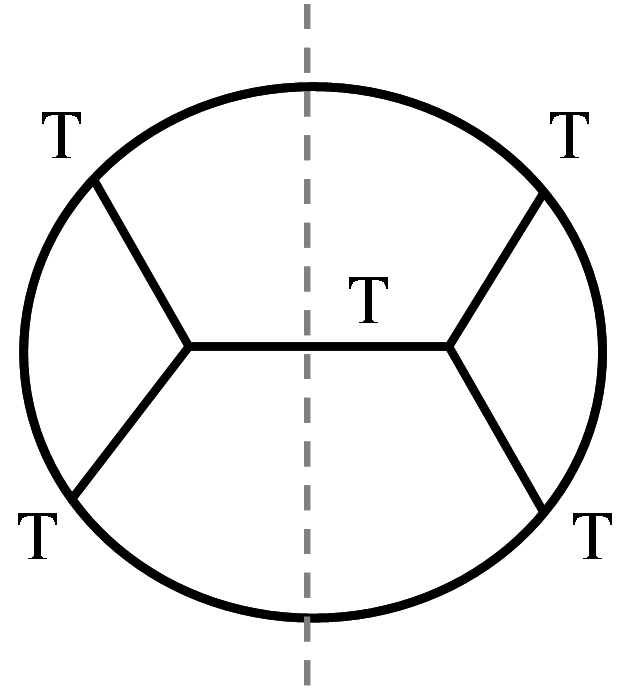
Figure 6: The tree-level exchange diagram for the $\mathcal{N}=4$ stress tensor multiplet.

The double-discontinuity is particularly simple to compute in holographic theories, as it is saturated at tree-level by exchange of a finite number of light single-trace operators. In some sense the dispersion relation give novel “closed form” expressions for tree-level holographic correlators as an integral over conformal blocks.

For illustration, consider the correlator of stress-tensor multiplets in planar $\mathcal{N}=4$ at large ’t Hooft coupling, dual to tree-level gravity in AdS${}_{5}\times S_{5}$. We follow the notation of Alday:2017vkk . (In short: because of supersymmetry, the stress tensor lies in a supermultiplet which includes scalars of dimensions $\Delta_{i}=2$ in the $[0,2,0]$ representation of the SU(4)_R global symmetry. We study the correlation functions of these scalars, projected onto the $s$-channel $[0,4,0]$ representation, which is known to determine all other representations. This projection has good high-energy behavior, allowing to use the unsubtracted dispersion relation.) The double-discontinuity in this limit is saturated by exchange of a single $t$-channel (super)conformal block corresponding to the stress tensor multiplet, or graviton exchange in the bulk (fig. 6); it admits a particularly concise form Aprile:2017bgs ; Alday:2017vkk :

$${\rm dDisc}[\mathcal{G}(w,{\bar{w}})]^{(1)}={\rm dDisc}\left[\frac{1}{1-{\bar{w}}}\right]\times\left(\frac{w^{2}-4w^{3}+3w^{4}-2w^{4}\log w}{(1-w)^{4}}\equiv X(w)\right).$$ (97)

The correlator itself is the only single-value function with this double-discontinuity (and correct Regge behavior) and is given as DHoker:1999jke ; Arutyunov:2000py (see Dolan:2000ut for the $\bar{D}$ functions):

$$\mathcal{G}(z,{\bar{z}})^{(1)} =\frac{u^{2}}{v}-u^{4}\bar{D}_{2422}(u,v),$$ (98)

$$\bar{D}_{2422} =\partial_{u}\partial_{v}(1+u\partial_{v}+v\partial_{v})\Phi^{(1)}(u,v),$$

$$\Phi^{(1)}(u,v) =\frac{2{\rm Li}_{2}(z)-2{\rm Li}_{2}({\bar{z}})+\log[\frac{1-z}{1-{\bar{z}}}]\log(z{\bar{z}})}{(z-{\bar{z}})}.$$

We would like to see here how the dispersion relation reconstructs (98) starting from the elementary dDisc given above it.

First we note that the dDisc is naively zero (no branch cut), so it is really a sort of delta-function around ${\bar{w}}=1$. This can be seen explicitly from the keyhole contour in fig. 5: only the semi-circles survive. In fact it is possible to directly integrate numerically over the semi-circles and compare (successfully) with (98). Let us see how the integral could be done analytically. In fact, the two half-circles would precisely cancel each other were it not for the fact that the kernel has a log. So ${\rm dDisc}[1/(1-{\bar{w}})]$ is effectively $-2\pi^{2}$ times a sort of $\delta$-function which extracts the coefficient of $\log(1-{\bar{w}})$ in the kernel, and eq. (94) becomes

$$\mathcal{G}(z,{\bar{z}})^{(1)}=\int_{0}^{w_{\rm max}}dw\frac{\big{[}-2u^{2}(1-w)(u/w+1-v)\big{]}+\mbox{(u-channel)}}{\big{(}u^{2}-2wu(1+v)+w^{2}(1-v)^{2}\big{)}^{3/2}}\times X(w)$$ (99)

where $w_{\rm max}=\frac{u}{(1+\sqrt{v})^{2}}$ is where $\rho_{w}=\rho_{z}{\bar{\rho}_{z}}$. Adding the $u$-channel term simply cancels the $(1-v)$ term in the numerator, and doubles the remaining $u/w$ term. A comment is in order: the integration endpoint is a branch point of the denominator, so it appears that by shrinking the circles to get a $\delta$-function we have created a new divergence as $w=w_{\rm max}$. One can show that the proper treatment simply amounts to integrating $w$ itself on a keyhole, $\int_{0}^{w_{\rm max}}\mapsto\frac{1}{2}\int_{0}^{0}$, as in fig. 4a. The integral is then unambiguous, and can also be checked numerically (giving a nontrivial confirmation of the form of the dispersion relation).

The form of the integrand of eq. (99) makes manifest the fact that the integral gives a combination of dilogarithms and simpler functions — the most complicated part can be written in the form $\int d\log(\cdots)\log(w)$, to which standard integration algorithm can be applied, see for example Panzer:2014caa . (Since the square root has two branch points with respect to $w$, one has to first go to a double-cover where the square root is gone.) It could be interesting to use this method to help understand the functions which can appear at higher loops.

5.3 An integral relation between conformal blocks

The validity of the dispersion relation predicts a new relation between harmonic functions and the inverted block which enters the Lorentzian inversion formula (and accessorily rederive the latter). Recall the dispersion relation:

$$\mathcal{G}(z,{\bar{z}})=\int dwd{\bar{w}}\ K(w,{\bar{w}},z,{\bar{z}})\ {\rm dDisc}[\mathcal{G}(w,{\bar{w}})]+(t\leftrightarrow u)$$ (100)

The Euclidean inversion formula, in the conventions of Caron-Huot:2017vep , is:

$$c(J,\Delta)=N(J,\Delta)\int_{\rm Eucl}dzd{\bar{z}}\ \mu(z,{\bar{z}})\ F_{J,\Delta}(z,{\bar{z}})\ \mathcal{G}(z,{\bar{z}})$$ (101)

where the normalization is $N(J,\Delta)\equiv\frac{\Gamma(J+\frac{d-2}{2})\Gamma(J+\frac{d}{2})K_{J,\Delta}}{2\pi\Gamma(J+1)\Gamma(J+d-2)K_{J,d-\Delta}}$. Plugging eq. (100) inside eq. (101) gives:

$$\begin{aligned} &c(J,\Delta)=N(J,\Delta)\int dwd{\bar{w}}\ \mu(w,{\bar{w}})\ {\rm dDisc}[\mathcal{G}(w,{\bar{w}})]\times\\ &\int dzd{\bar{z}}\frac{\mu(z,{\bar{z}})}{\mu(w,{\bar{w}})}F_{J,\Delta}(z,{\bar{z}})K(w,{\bar{w}},z,{\bar{z}})+(t\leftrightarrow u)\end{aligned}$$ (102)

where we exchanged integration orders, and multiplied and divided by $\mu(w,{\bar{w}})$. This has precisely the form of the Lorentzian inversion formula (23): Euclidean inversion plus dispersion relation gives Lorentzian inversion. The interesting thing is that comparison reveals the following identity:

$$\boxed{G_{\Delta+1-d,J+d-1}(w,{\bar{w}})=\frac{4N(J,\Delta)}{\kappa_{J+\Delta}}\int_{\rm Eucl}dzd{\bar{z}}\frac{\mu(z,{\bar{z}})}{\mu(w,{\bar{w}})}F_{J,\Delta}(z,{\bar{z}})K(w,{\bar{w}},z,{\bar{z}})}$$ (103)

This is predicted to hold for any $d$, $J$, and $\Delta$. The integration is over the complex $z$ plane, i.e ${\bar{z}}=z^{*}$. This equation is the analog of the relation between the Legendre polynomials of the first and second kind (See table 1):

$$Q_{J}(x)=\frac{1}{2}\int_{-1}^{1}\frac{dyP_{J}(y)}{y-x}\ .$$ (104)

While we haven’t checked this relation in the general case, in appendix B we verify it in the special case that $d=2$ and $(a,b)=(0,\tfrac{1}{2})$. It would be interesting to understand the relationship between this identity and the light transform of Kravchuk:2018htv .

5.4 3D Ising model and analytic functionals

In the 3D Ising model, we now present numerical tests for the correlator of four $Z_{2}$-odd operators ($\langle\sigma\sigma\sigma\sigma\rangle$), and discuss a possible way to reorganize the crossing equations.

A straightforward exercise (if somewhat technical) is to numerically integrate the subtracted dispersion relation in eq. (93), using the OPE data tabulated in Simmons-Duffin:2016wlq to compute ${\rm dDisc}[\mathcal{G}]$ as a sum over $t$-channel blocks. It is important conceptually that the $t$-channel OPE commutes with the dispersion relation. The basic reason is that the interior of the integration region, $w,{\bar{w}}\in(0,1)$, lies within the convergence radius of the OPE. It is also important to be careful near endpoints which lie at the boundary of convergence Rychkov:2017tpc . In our case these are the collinear limit $w=0$ and Regge corner $w,{\bar{w}}\to 0$. Due to absolute convergence of the (subtracted) kernel against the full correlator, and thanks to positivity of the OPE, we expect that the operations safely commute.

The most important numbers (with uncertainty in the last digit, see Simmons-Duffin:2016wlq ) are:

$$\Delta_{\sigma}=0.518149,\qquad\Delta_{\epsilon}=1.41263,\qquad f_{\sigma\sigma\epsilon}=1.051854.$$ (105)

We used the 3D$\to$2D dimensional reduction formulas of ref. Hogervorst:2016hal to efficiently compute the 3D conformal blocks. Breaking the contributions into those of dominant operators and families, we find for example the correlator at a specific point $(z,{\bar{z}})=(\tfrac{1}{2},\tfrac{1}{4})$

$$v^{\Delta_{\sigma}}\mathcal{G}(\tfrac{1}{2},\tfrac{1}{4}) = 0.36878_{1}+0.29685_{\epsilon}+0.16493_{T}+0.00568_{[\sigma\sigma]_{0,\geq 4}}+0.00030_{\epsilon^{\prime}}+0.00018$$ (106)

$$\approx 0.83672$$

where the superscript label the cross-channel operator(s), and the last term collects all the other operators ($[\sigma\sigma]_{1}$ and $[\epsilon\epsilon]_{0}$ families) recorded in Simmons-Duffin:2016wlq . Some comments are in order about the lowest twist trajectory $[\sigma\sigma]_{0}$. We separated the spin-2 contribution (stress-tensor $T$) from the others of spin $J\geq 4$. Naively, one may have expect the whole trajectory to be suppressed by a $\sin^{2}(\pi(\tau/2-\Delta_{\sigma}))$ factor, however, as explained below eq. (93), the subtracted dispersion relation involves ${\rm dDisc}[\mathcal{G}u/v]$ which prevents that cancelation for the lowest twist (the usual suppressions still operate for $[\sigma\sigma]_{1}$). As indicated in fig. 7a, by evaluating the contribution of these operators up to spins $O(20)$ and fitting to a power-law, we find that we can accurately resum the trajectory (the fit in the figure used spins 20,22,24).

Performing the similar calculation at crossing-related points $(\tfrac{1}{2},\tfrac{3}{4})$ we find:

$$v^{\Delta_{\sigma}}\mathcal{G}(\tfrac{1}{2},\tfrac{3}{4}) = 0.61635_{1}+0.19655_{\epsilon}+0.02951_{T}-0.00597_{[\sigma\sigma]_{0,\geq 4}}+0.00011_{\epsilon^{\prime}}+0.00003$$ (107)

$$\approx 0.83659.$$

The difference of these two numbers is a crossing equation, satisfied at the $10^{-4}$ level:

$$X(\tfrac{1}{2},\tfrac{1}{4})=-0.00013,\qquad X(z,{\bar{z}})\equiv\left(v^{\Delta_{\sigma}}\mathcal{G}(u,v)-u^{\Delta_{\sigma}}\mathcal{G}(v,u)\right).$$ (108)

For comparison, calculating the same correlators $vG$ at these particular points using the Euclidean OPE (and same OPE coefficients), we find a compatible value $vG=0.83657$ (with a change of $\pm 2$ in the last digit between the two crossing-related positions). The agreement convincingly shows that the dispersion relation indeed reconstructs the correlator. It is presently not clear whether the (small, but significant) $10^{-4}$ error in (106) is due to numerical integration or truncation of the spectrum.

Conceptually, one may be concerned that the sensitivity to the lowest twist trajectory means that the formula requires more than the absorptive part. However, in practice, the lowest-twist data is particularly well understood from the Lorentzian inversion formula. A very crude approximation (simply feeding the identity and $\epsilon$ into the inversion formula, following Albayrak:2019gnz ), for example reproduces the OPE coefficients of Simmons-Duffin:2016wlq to per-mil accuracy; we used this approximation in the above, for spins 12 and higher. Conceptually, one may view the first four contributions in eq. (106) as accurately parametrized (to per-mil level) simply by three parameters: $(\Delta_{\sigma},\Delta_{\epsilon},f_{\sigma\sigma\epsilon})$.

It is amusing to try to constraint this crude model, for example for a given $\Delta_{\sigma}$ one can find $(\Delta_{\epsilon},f_{\sigma\sigma\epsilon})$ which minimizes the error in the crossing relation (and in the twist of the stress tensor). Preliminary investigations yield a curve(s) passing through the numerical bootstrap solution (105), with values of $\Delta_{\epsilon}$ differing by less than $\pm 0.01$ when considering different crossing equations (we did not observe any kink). Possibly, to close the system and also fix $\Delta_{\sigma}$ by such methods, one will need to consider mixed correlators.

$$\begin{array}[]{cc}\raisebox{8.53581pt}{\includegraphics[width=199.16928pt]{power_law.pdf}}&\includegraphics[width=227.62204pt]{functional.pdf}\\ \rm(a)&\rm(b)\end{array}$$

Figure 7: (a) High-spin tail of the contribution of the lowest-twist family $[\sigma\sigma]_{0,J}$ to the correlator in eq. (106). Operators of spin $28$ and higher were resummed using the power-law fit. (b) “Bootstrap functional” obtained by evaluating the contribution of spin-0 and spin-2 exchanged operators of dimension $\Delta$ to the dispersion integral $X(\tfrac{1}{2},\tfrac{1}{4})$ in eq. (108), with external dimensions fixed to $\Delta_{\sigma}$. A rescaling envelope was applied. Note that the curves have double zeros at non-leading double-twist dimensions.

It is interesting that the contributions of individual blocks are very different between the Euclidean OPE and dispersion relation: the dispersion relation is not a term-wise rewriting of the OPE. This becomes particularly sharp if we plot the contribution to a crossing equation, say $X(\tfrac{1}{2},\tfrac{1}{4})$, from a given cross-channel operator. This gives a “bootstrap functional”, shown in fig. 7b, which must be orthogonal to the OPE data. That particular functional has double zeros at all (non-leading) double-twist operators, and is mostly positive (with the exception of the identity contribution, and some lowest-twist operators at high spin, not shown). In contrast, Euclidean functionals display no such oscillatory behavior.

One can create a few more functionals of this type. For example, $t{\leftrightarrow}u$ crossing symmetry is not manifest because of the subtraction (93), giving a nontrivial constraint:

$$\tilde{X}(z,{\bar{z}})\equiv\mathcal{G}(z,{\bar{z}})-\mathcal{G}\big{(}\tfrac{z}{z-1},\tfrac{{\bar{z}}}{{\bar{z}}-1}\big{)}=0.$$ (109)

A special case includes the Regge limit, for example the correlator should be real for imaginary $\rho$’s:

$${\rm Im}\ \mathcal{G}(\rho_{z}=ia,{\bar{\rho}_{z}}=-ib)=0,\qquad(0<a<1<b\mbox{ real}).$$ (110)

Such functionals will likely not form a complete basis (all have double zeros at the double-twists, unlike some of those in Mazac:2016qev ), but it would be interesting to compare and perhaps combine them with other functionals like those found in Paulos:2019gtx ; Mazac:2019shk .

6 Conclusion

In this work we obtained a dispersion relation for four-point correlators of conformal field theories, reconstructing them from an “absorptive part” (double discontinuity). It’s kernel (given in eqs. (34), (38) and (55)) was found by explicitly resuming the Lorentzian inversion formula of Caron-Huot:2017vep ; Simmons-Duffin:2017nub ; Kravchuk:2018htv . For non-equal external operators, a differential equation was obtained, eq. (76). A subtracted dispersion relation, in eq. (93), overcomes the limitations of the inversion formula fully reconstructs the correlators in an arbitrary (unitary) conformal field theories. Various tests were performed, including in holographic theories and the 3D Ising model.

The dispersion relation holds for $d\geq 2$. For $d=1$ there is only one cross ratio $z$, and thus one could expect a simpler dispersion relation. Ref. Mazac:2018qmi obtained a crossing symmetric inversion formula in $d=1$. The kernel in this inversion formula is quite complicated for general scaling dimensions, precisely because it needs to give rise to a crossing symmetric correlator. Combining a known $d=1$ inversion formula with the methods that we presented in this note, one can obtain a $d=1$ dispersion relation New containing the double-discontinuity. It is also possible New to obtain dispersion relations for boundary/defect CFTs by starting from the Lorentzian inversion formulas of Liendo:2019jpu ; Mazac:2018biw . Investigating the flat space limit of the dispersion relation would also be interesting, as well as comparison with momentum space approaches (for example Gillioz:2016jnn ).

In our view, the most appealing feature is that the “absorptive part” (or dDisc) on which the dispersion relation feeds can often be rather accurately approximated by just the simplest exchanges, as discussed below eq. (108). This strongly suggests that this is the right data around which to build a systematic expansion. Our hope is that the dispersion relation presented here will help achieve that, as crossing symmetry can now be directly formulated as a constraint on the dDisc. After subtracting the simplest exchanges, the remainder of the dDisc should be a small, positive, and regular function on a square ($0{<}z,{\bar{z}}{<}1$). Finding how to “close” the equations and bootstrap this function is in our view a key next question.

Appendix A Identities for spin sums

In this appendix we collect some of mathematical results that we use in the main text. In Eq. 43 we used the following $J$ sum which contains 2 hypergeometric functions, which one can easily check by series expanding in $w$:

$$\begin{aligned} &\sum_{J=0}^{\infty}\frac{k_{-2J-2m^{\prime}}(z)k_{2J+2m^{\prime}+2}(w)}{1+\delta_{J,0}}\\ &=\frac{zw}{z-w}\Big{(}k_{-2m^{\prime}}(z)k_{2m^{\prime}}(w)-\frac{m^{\prime 2}k_{-2m^{\prime}+2}(z)k_{2m^{\prime}+2}(w)}{4(4m^{\prime 2}-1)}\Big{)}-\frac{k_{-2m^{\prime}}(z)k_{2m^{\prime}+2}(w)}{2}\\ &=\frac{1}{2m^{\prime}+1}\left[\frac{zw}{z-w}\Big{(}(1-w)\partial_{w}-(1-z)\partial_{z}\Big{)}-\frac{1}{2}\right]k_{-2m^{\prime}}(z)k_{2m^{\prime}+2}(w).\end{aligned}$$ (111)

The idea behind the first equality is that $(1/z-1/w)$ times the summand on the first line can be rewritten, using hypergeometric identities, in terms of $k$-functions with shifted arguments so as to turn the sum into a telescopic one. The second line similarly re-interpret shifted $k$-functions in terms of derivatives on simple term. The above identity is valid for arbitrary offset $m^{\prime}$, but $a=b=0$. For non-zero $a$ and $b$, the second line form of the above identity becomes more complicated, but the derivative form remains unchanged:

$$\begin{aligned} &\sum_{J=0}^{\infty}\frac{k_{-2J-2m^{\prime}}^{(a,b)}(z)k_{2J+2m^{\prime}+2}^{(a,b)}(w)}{1+\delta_{J,0}}\\ &=\frac{1}{2m^{\prime}+1}\left[\frac{zw}{z-w}\Big{(}(1-w)\partial_{w}-(1-z)\partial_{z}\Big{)}-\frac{1}{2}\right]k_{-2m^{\prime}}^{(a,b)}(z)k_{2m^{\prime}+2}^{(a,b)}(w).\end{aligned}$$ (112)

Introducing the differential operator (the subscripts stands for $d=2$):

$$\mathcal{D}_{2}\equiv\frac{zw}{z-w}\Big{(}(1-w)\partial_{w}-(1-z)\partial_{z}\Big{)}+\frac{{\bar{z}}w}{{\bar{z}}-w}\Big{(}(1-w)\partial_{w}-(1-{\bar{z}})\partial_{{\bar{z}}}\Big{)}-1,$$ (113)

this allows us to rewrite the sum (43) in a concise form:

$$\sum_{J=0}^{\infty}\frac{k_{-2J-2m^{\prime}-2a}(z)k_{-2m^{\prime}-2a}({\bar{z}})k_{-2m^{\prime}-2a}({\bar{w}})(k_{2J+2m^{\prime}+2+2a}(w)}{1+\delta_{J,0}}+(z{\leftrightarrow}{\bar{z}})$$ (114)

$$=\frac{1}{2m^{\prime}+1}\mathcal{D}_{2}\Big{[}k_{-2m^{\prime}}(z)k_{-2m^{\prime}}({\bar{z}})k_{-2m^{\prime}}({\bar{w}})k_{2m^{\prime}+2}(w)\Big{]}.$$ (115)

Appendix B Inverted block from harmonic function when $a=0$, $b=\frac{1}{2}$

In order to check the integral relation in Eq. 103, we fix $d=2$ and $a=0$, $b=\frac{1}{2}$. In this case the dispersion relation contains only the contact term $K_{C}$ and not the bulk term $K_{B}$, as we saw in Eq. 79. Thus Eq. 103 becomes:

$$\frac{\frac{\pi}{2}\kappa_{J+2-\Delta}}{1+\delta_{J,0}}G_{\Delta-1,J+1}(w,{\bar{w}})=\int_{\rm Eucl}dzd{\bar{z}}\frac{\mu(z,{\bar{z}})}{\mu(w,{\bar{w}})}F_{J,\Delta}(z,{\bar{z}})\delta(\rho_{w}-{\bar{\rho}_{w}}\rho_{z}{\bar{\rho}_{z}})K_{C}\frac{d\rho_{w}}{dw}$$ (116)

For $a=0$, $b=\frac{1}{2}$ the ${}_{2}F_{1}$’s of the conformal block basically simplifies to powers of $\rho$:

$$G_{J,\Delta}(z,{\bar{z}})=\frac{1}{1+\delta_{J,0}}(k_{\Delta-J}(z)k_{\Delta+J}({\bar{z}})+k_{\Delta+J}(z)k_{\Delta-J}({\bar{z}}))$$

$$=\frac{2^{2\Delta}}{1+\delta_{J,0}}\frac{(\rho_{z})^{\frac{\Delta-J}{2}}({\bar{\rho}_{z}})^{\frac{\Delta+J}{2}}+(\rho_{z})^{\frac{\Delta+J}{2}}({\bar{\rho}_{z}})^{\frac{\Delta-J}{2}}}{(1-\rho_{z})(1-{\bar{\rho}_{z}})}=\frac{2^{2\Delta}r^{\Delta}(e^{i\theta J}+e^{-i\theta J})}{(1+\delta_{J,0})|1-re^{i\theta}|^{2}}$$ (117)

where in the last equality we changed to polar coordinates $\rho_{z}=re^{i\theta}$, and used the fact that in Euclidean we have $\bar{\rho}_{z}=\rho^{*}_{z}$. Similarly, we can write $K_{C}$ and the inverted block in polar coordinates. Plugging these ingredients back in Eq. 116, we can now check that Eq. 116 gives a correct result:

$$\frac{1}{\frac{\pi}{2}\kappa_{J+2-\Delta}G_{\Delta-1,J+1}(w,{\bar{w}})}\int_{\rm Eucl}dzd{\bar{z}}\frac{\mu(z,{\bar{z}})}{\mu(w,{\bar{w}})}F_{J,\Delta}(z,{\bar{z}})\delta(\rho_{w}-{\bar{\rho}_{w}}\rho_{z}{\bar{\rho}_{z}})K_{C}\frac{d\rho_{w}}{dw}$$

$$=\frac{\rho_{w}^{\frac{5}{2}}{\bar{\rho}_{w}}^{-\frac{3}{2}}(1-\rho_{w}{\bar{\rho}_{w}})(\rho_{w}\bar{\rho}_{w})^{\frac{-J}{2}}}{(\rho_{w})^{\frac{2-\Delta}{2}}({\bar{\rho}_{w}})^{\frac{\Delta}{2}}+(\rho_{w})^{\frac{\Delta}{2}}({\bar{\rho}_{w}})^{\frac{2-\Delta}{2}}}\int_{0}^{2\pi}d\theta\int_{0}^{\infty}dr\frac{r^{\Delta}+r^{2-\Delta}}{4\pi r^{5}}\frac{(e^{i\theta J}+e^{-i\theta J})\delta(r-\sqrt{\frac{\rho_{w}}{{\bar{\rho}_{w}}}})}{|\sqrt{\rho_{w}{\bar{\rho}_{w}}}-e^{-i\theta}|^{2}}$$

$$=\frac{(1-\rho_{w}{\bar{\rho}_{w}})}{4\pi(\rho_{w}\bar{\rho}_{w})^{\frac{J}{2}}}\int_{0}^{2\pi}\frac{(e^{i\theta J}+e^{-i\theta J})d\theta}{|\sqrt{\rho_{w}{\bar{\rho}_{w}}}-e^{-i\theta}|^{2}}$$

$$=\frac{(1-\rho_{w}{\bar{\rho}_{w}})}{4\pi i(\rho_{w}\bar{\rho}_{w})^{\frac{J}{2}}}\int_{|Z|=1}\frac{(Z^{J-1}+Z^{-J-1})dZ}{(Z-\sqrt{\rho_{w}{\bar{\rho}_{w}}})(Z^{-1}-\sqrt{\rho_{w}{\bar{\rho}_{w}}})}=1$$ (118)

Where in the third line we performed the $r$ integral over the delta function, in the third line wrote the remaining $\theta$ integral as a contour integral in the complex $Z\equiv e^{i\theta}$ plane, and then used the residue theorem in the complex $Z$ plane to get 1.

References

• (1) R. Rattazzi, V. S. Rychkov, E. Tonni and A. Vichi, Bounding scalar operator dimensions in 4D CFT, JHEP 12 (2008) 031, [0807.0004].
• (2) S. El-Showk, M. F. Paulos, D. Poland, S. Rychkov, D. Simmons-Duffin and A. Vichi, Solving the 3D Ising Model with the Conformal Bootstrap, Phys. Rev. D86 (2012) 025022, [1203.6064].
• (3) D. Simmons-Duffin, The Lightcone Bootstrap and the Spectrum of the 3d Ising CFT, JHEP 03 (2017) 086, [1612.08471].
• (4) D. Poland, S. Rychkov and A. Vichi, The Conformal Bootstrap: Theory, Numerical Techniques, and Applications, 1805.04405.
• (5) Z. Komargodski and A. Zhiboedov, Convexity and Liberation at Large Spin, JHEP 11 (2013) 140, [1212.4103].
• (6) A. L. Fitzpatrick, J. Kaplan, D. Poland and D. Simmons-Duffin, The Analytic Bootstrap and AdS Superhorizon Locality, JHEP 12 (2013) 004, [1212.3616].
• (7) L. F. Alday and A. Zhiboedov, An Algebraic Approach to the Analytic Bootstrap, JHEP 04 (2017) 157, [1510.08091].
• (8) L. F. Alday, Large Spin Perturbation Theory for Conformal Field Theories, Phys. Rev. Lett. 119 (2017) 111601, [1611.01500].
• (9) A. Martin, Scattering Theory: Unitarity, Analyticity and Crossing, Lect. Notes Phys. 3 (1969) 1–117.
• (10) R. J. Eden, P. V. Landshoff, D. I. Olive and J. C. Polkinghorne, eds., The analytic S-matrix. Cambridge University Press, 1966.
• (11) G. R. Screaton, ed., Dispersion Relations. Interscience publishers inc., 1961.
• (12) M. A. Shifman, ed., Vacuum structure and QCD sum rules. Amsterdam, Netherlands: North-Holland, 1992.
• (13) Z. Komargodski and A. Schwimmer, On Renormalization Group Flows in Four Dimensions, JHEP 12 (2011) 099, [1107.3987].
• (14) Z. Bern, L. J. Dixon, D. C. Dunbar and D. A. Kosower, One loop n point gauge theory amplitudes, unitarity and collinear limits, Nucl. Phys. B425 (1994) 217–260, [hep-ph/9403226].
• (15) R. Britto, F. Cachazo and B. Feng, Generalized unitarity and one-loop amplitudes in N=4 super-Yang-Mills, Nucl. Phys. B725 (2005) 275–305, [hep-th/0412103].
• (16) R. Britto, F. Cachazo, B. Feng and E. Witten, Direct proof of tree-level recursion relation in Yang-Mills theory, Phys. Rev. Lett. 94 (2005) 181602, [hep-th/0501052].
• (17) H. Elvang and Y.-t. Huang, Scattering Amplitudes, 1308.1697.
• (18) S. Caron-Huot, Analyticity in Spin in Conformal Theories, JHEP 09 (2017) 078, [1703.00278].
• (19) D. Simmons-Duffin, D. Stanford and E. Witten, A spacetime derivation of the Lorentzian OPE inversion formula, JHEP 07 (2018) 085, [1711.03816].
• (20) P. Kravchuk and D. Simmons-Duffin, Light-ray operators in conformal field theory, 1805.00098.
• (21) L. F. Alday, J. Henriksson and M. van Loon, Taming the epsilon-expansion with large spin perturbation theory, JHEP 07 (2018) 131, [1712.02314].
• (22) L. F. Alday, J. Henriksson and M. van Loon, An alternative to diagrams for the critical O(N) model: dimensions and structure constants to order 1/N2, 1907.02445.
• (23) S. Albayrak, D. Meltzer and D. Poland, More Analytic Bootstrap: Nonperturbative Effects and Fermions, 1904.00032.
• (24) C. Cardona, S. Guha, S. K. Kanumilli and K. Sen, Resummation at finite conformal spin, JHEP 01 (2019) 077, [1811.00213].
• (25) W. Li, Closed-form expression for cross-channel conformal blocks near the lightcone, 1906.00707.
• (26) J. Liu, E. Perlmutter, V. Rosenhaus and D. Simmons-Duffin, d-dimensional SYK, AdS Loops, and 6j Symbols, 1808.00612.
• (27) L. F. Alday and S. Caron-Huot, Gravitational S-matrix from CFT dispersion relations, 1711.02031.
• (28) S. Caron-Huot and A.-K. Trinh, All tree-level correlators in $=$ supergravity: hidden ten-dimensional conformal symmetry, JHEP 01 (2019) 196, [1809.09173].
• (29) M. Lemos, P. , M. Meineri and S. Sarkar, Universality at large transverse spin in defect CFT, JHEP 09 (2018) 091, [1712.08185].
• (30) L. Iliesiu, M. Kologlu, R. Mahajan, E. Perlmutter and D. Simmons-Duffin, The Conformal Bootstrap at Finite Temperature, 1802.10266.
• (31) A. Bissi, P. Dey and T. Hansen, Dispersion Relation for CFT Four-Point Functions, 1910.04661.
• (32) A. Martin, Unitarity and high-energy behavior of scattering amplitudes, Phys. Rev. 129 (1963) 1432–1436.
• (33) M. F. Paulos, J. Penedones, J. Toledo, B. C. van Rees and P. Vieira, The S-matrix bootstrap II: two dimensional amplitudes, JHEP 11 (2017) 143, [1607.06110].
• (34) M. F. Paulos, J. Penedones, J. Toledo, B. C. van Rees and P. Vieira, The S-matrix Bootstrap III: Higher Dimensional Amplitudes, 1708.06765.
• (35) M. Froissart, Phys. Rev. 123, 1053 (1961) .
• (36) V. N. Gribov, Zh. Eksp. Teor. Fiz. Sov. Phys. JETP 14, 478,1395 (1961) .
• (37) M. Hogervorst and S. Rychkov, Radial Coordinates for Conformal Blocks, Phys. Rev. D87 (2013) 106004, [1303.1111].
• (38) V. K. Dobrev, V. B. Petkova, S. G. Petrova and I. T. Todorov, Dynamical Derivation of Vacuum Operator Product Expansion in Euclidean Conformal Quantum Field Theory, Phys. Rev. D13 (1976) 887.
• (39) V. K. Dobrev, G. Mack, V. B. Petkova, S. G. Petrova and I. T. Todorov, Harmonic Analysis on the n-Dimensional Lorentz Group and Its Application to Conformal Quantum Field Theory, Lect. Notes Phys. 63 (1977) 1–280.
• (40) M. S. Costa, V. Goncalves and J. Penedones, Conformal Regge theory, JHEP 12 (2012) 091, [1209.4355].
• (41) N. Gromov, V. Kazakov and G. Korchemsky, Exact Correlation Functions in Conformal Fishnet Theory, JHEP 08 (2019) 123, [1808.02688].
• (42) G. G.N. Watson, Notes on Generating Functions of Polynomials: (3) Polynomials of Legendre and Gegenbauer, Journal of the London Mathematical Society s1-8 (1933) .
• (43) A. Baranov, On Series Containing Products of Legendre Polynomials, Mathematical Notes, vol. 80, no. 2, 2006. Translated from Matematicheskie Zametki, vol. 80, no. 2, 2006, .
• (44) H. van Haeringen, A class of sums of Gegenbauer functions: Twenty-four sums in closed form, Journal of Mathematical Physics 27, 938 (1986) .
• (45) J. S. M. Rahman, M, Sums of products of ultraspherical functions, Journal of Mathematical Physics 26, 627 (1985) .
• (46) F. Aprile, J. M. Drummond, P. Heslop and H. Paul, Quantum Gravity from Conformal Field Theory, JHEP 01 (2018) 035, [1706.02822].
• (47) E. D’Hoker, D. Z. Freedman, S. D. Mathur, A. Matusis and L. Rastelli, Extremal correlators in the AdS / CFT correspondence, hep-th/9908160.
• (48) G. Arutyunov and S. Frolov, Four point functions of lowest weight CPOs in N=4 SYM(4) in supergravity approximation, Phys. Rev. D62 (2000) 064016, [hep-th/0002170].
• (49) F. A. Dolan and H. Osborn, Conformal four point functions and the operator product expansion, Nucl. Phys. B599 (2001) 459–496, [hep-th/0011040].
• (50) E. Panzer, Algorithms for the symbolic integration of hyperlogarithms with applications to Feynman integrals, Comput. Phys. Commun. 188 (2015) 148–166, [1403.3385].
• (51) J. Qiao and S. Rychkov, Cut-touching linear functionals in the conformal bootstrap, JHEP 06 (2017) 076, [1705.01357].
• (52) M. Hogervorst, Dimensional Reduction for Conformal Blocks, JHEP 09 (2016) 017, [1604.08913].
• (53) D. Mazac, Analytic bounds and emergence of AdS2 physics from the conformal bootstrap, JHEP 04 (2017) 146, [1611.10060].
• (54) M. F. Paulos, Analytic Functional Bootstrap for CFTs in $d>1$, 1910.08563.
• (55) D. Maz ˇc, L. Rastelli and X. Zhou, A Basis of Analytic Functionals for CFTs in General Dimension, 1910.12855.
• (56) D. Mazac, A Crossing-Symmetric OPE Inversion Formula, 1812.02254.
• (57) D. Carmi and A. Vichi, More on CFT dispersion relations, Work in progress​ .
• (58) P. Liendo, Y. Linke and V. Schomerus, A Lorentzian inversion formula for defect CFT, 1903.05222.
• (59) D. Mazac, L. Rastelli and X. Zhou, An Analytic Approach to BCFT, 1812.09314.
• (60) M. Gillioz, X. Lu and M. A. Luty, Scale Anomalies, States, and Rates in Conformal Field Theory, JHEP 04 (2017) 171, [1612.07800].