Superadiabatic thermalization of a quantum oscillator by engineered dephasing

Abstract

Fast nonadiabatic control protocols known as shortcuts to adiabaticity have found a plethora of applications, but their use has been severely limited to speeding up the dynamics of isolated quantum systems. We introduce shortcuts for open quantum processes that make possible the fast control of Gaussian states in non-unitary processes. Specifically, we provide the time modulation of the trap frequency and dephasing strength that allow preparing an arbitrary thermal state in a finite time. Experimental implementation can be done via stochastic parametric driving or continuous measurements, readily accessible in a variety of platforms.

The fast control of quantum systems with high-fidelity is broadly acknowledged as a necessity to advance quantum science and technology. In this context, techniques known as shortcuts to adiabaticity (STA) have provided an alternative to adiabatic driving with a wide variety of applications Torrontegui et al. (2013). STA tailor excitations in nonadiabatic processes to prepare a given state in a finite time, without the requirement of slow driving. The experimental demonstration of STA was pioneered in a trapped thermal cloud Schaff et al. (2010), soon followed by implementations in Bose-Einstein condensates Schaff et al. (2011), cold atoms in optical lattices Bason et al. (2012) and low-dimensional quantum fluids Rohringer et al. (2015). More recently, STA have also been applied to Fermi gases, both in the non-interacting and unitary regimes Deng et al. (2018a, b). Beyond the realm of cold atoms, STA have been demonstrated in quantum optical systems Du et al. (2016), trapped ions An et al. (2016), nitrogen vacancy-centers Zhang et al. (2013), and superconducting qubits Wang et al. (2018); Zhang et al. (2018). Their application is not restricted to quantum systems and classical counterparts exist Jarzynski (2013); Deffner et al. (2014), of relevance, e.g., to colloidal systems Schmiedl and Seifert (2007).

A variety of related control techniques fall under the umbrella of STA. Prominent examples include counter-diabatic or transitionless quantum driving Demirplak and Rice (2003, 2005); Berry (2009), the fast-forward technique Masuda and Nakamura (2009); Masuda et al. (2014), reverse-engineered dynamics using Lewis-Riesenfeld invariants Chen et al. (2010), as well as the use of dynamical scaling laws Muga et al. (2009); del Campo (2011, 2013); Deffner et al. (2014), Lax pairs Okuyama and Takahashi (2016), variational methods Sels and Polkovnikov (2017) and Floquet engineering Claeys et al. (2019). The use of STA in the quantum domain is severely limited to isolated systems, in which sources of noise and decoherence are considered an unwanted perturbation Calzetta (2018); Levy et al. (2018). Applications to finite-time thermodynamics have thus been limited to the speedup of strokes in which the working substance is in isolation and decoupled from any external reservoir Deng et al. (2018b).

Controlling heating and cooling processes would pave the way to the realization of superadiabatic heat engines and refrigerators based, e.g. in an Otto or Carnot quantum cycle Feldmann and Kosloff (2006); Deng et al. (2013); del Campo et al. (2014); Beau et al. (2016); Villazon et al. (2019); Dann and Kosloff (2019). Hence, the possibility to speed up the dynamics of open quantum systems is highly desirable in view of applications to cooling, and more generally, in finite-time thermodynamics. In this context, the nonadiabatic control of composite and open quantum systems using STA remains an exciting open problem on which few results are available Vacanti et al. (2014); Duncan and del Campo (2018); Dann et al. (2019); Villazon et al. (2019); Dann and Kosloff (2019); Alipour et al. (2019).

In this work, we introduce STA with open dynamics and apply them to the superadiabatic cooling and heating of a thermal harmonic oscillator. We show that the required control protocols are local and involve only the driving of the trap frequency and the dephasing strength. They can be achieved using stochastic parametric driving, thus harnessing noise as a resource.

Model.— We shall consider a single particle in a driven harmonic trap, with Hamiltonian

$$\hat{H}_{t}=\frac{1}{2m}\hat{p}^{2}+\frac{1}{2}m\omega_{t}^{2}\hat{x}^{2},$$ (1)

and a density matrix evolving according to a master equation of the form

$$\frac{d\rho_{t}}{dt}=-\frac{i}{\hbar}[\hat{H}_{t},\rho_{t}]-\gamma_{t}[\hat{x},[\hat{x},\rho_{t}]],$$ (2)

the derivation of which will be provided below. The case with constant dephasing strength $\gamma$ admits the Lindblad form with position operator $\hat{x}$ as the single Hermitian Lindblad operator. This naturally arises as the high-temperature limit of quantum Brownian motion. The dynamics with an arbitrary time-dependence $\gamma_{t}$ is generally non-Markovian. We shall show how a time-inhomogeneous Markovian dynamics Rivas et al. (2014), corresponding to $\gamma_{t}>0$, can be engineered by tailoring noise as a resource. The dynamics along the process is assumed to remain Gaussian, with a density matrix in coordinate space of the form

$$\rho_{t}(x,x^{\prime})=N_{t}\,e^{-A_{t}(x^{2}+x^{\prime 2})+iB_{t}(x^{2}-x^{\prime 2})-2C_{t}xx^{\prime}},$$ (3)

where $A_{t},B_{t},C_{t}$ are time-dependent coefficients to be determined from the master equation, $N_{t}=\sqrt{2(A_{t}+C_{t})/\pi}$ being the normalization factor. This form includes coherences during the dynamics, and represents a family of dynamical processes that, as shown below, allows for a fast and controlled thermalization.

As a relevant example, we consider the driving in a finite time $t_{f}$ of an initial thermal state, parameterized by the trap frequency and inverse temperature $(\omega_{0},\beta_{0})$, to a different thermal state with $(\omega_{f},\beta_{f})$. For the Gaussian variational Ansatz (3) to describe the exact dynamics of the master equation (2), the following consistency equations are to be satisfied (see App. B)

$$\dot{B}_{t} =\frac{2\hbar}{m}(A_{t}^{2}-B_{t}^{2}-C_{t}^{2})-\frac{m\omega_{t}^{2}}{2\hbar},$$ (4a)

$$0 =\dot{A}_{t}+\frac{4\hbar}{m}A_{t}B_{t}-\gamma_{t}=\dot{C}_{t}+\frac{4\hbar}{m}B_{t}C_{t}+\gamma_{t}.$$ (4b)

The parameter $2\hbar B_{t}/m=-(\dot{A}_{t}+\dot{C}_{t})/(2(A_{t}+C_{t}))\equiv\Omega_{t}$ is homogenous to a frequency, and directly follows from these equations. The boundary conditions are given from the initial and final states, that we choose to be thermal. As detailed in App. A, it follows that $A_{0}=\frac{m\omega_{0}}{2\hbar}\coth(\hbar\omega_{0}\beta_{0})$, $B_{0}=0$ and $C_{0}=-m\omega_{0}/\big{(}2\hbar\sinh(\hbar\omega_{0}\beta_{0})\big{)}$. Similarly, for the final state to be thermal, the coefficients at time $t_{f}$ should reduce to the values $A_{f}=\frac{m\omega_{f}}{2\hbar}{\rm coth}(\hbar\omega_{f}\beta_{f})$, $B_{f}=0$ and $C_{f}=-m\omega_{f}/\big{(}2\hbar\sinh(\hbar\omega_{f}\beta_{f})\big{)}$. The initial and final states being taken as equilibrium states, they are stationary. This imposes the additional boundary conditions $\dot{A}_{0/f}=\dot{B}_{0/f}=\dot{C}_{0/f}=0$. We also require that $\ddot{A}_{0/f}=\ddot{B}_{0/f}=\ddot{C}_{0/f}=0$ at initial and final time—the latter conditions are auxiliary, but guarantee a smooth variation of $\omega_{t}$ and $\gamma_{t}$.

A protocol speeding up the evolution from the thermal state characterized by $(\omega_{0},\beta_{0})$ to $(\omega_{f},\beta_{f})$ is obtained by explicitly specifying both the time-dependence of $\gamma_{t}$ and $\omega_{t}$, as directly given by the consistency equation (4), according to

$$\omega^{2}_{t} = \frac{4\hbar^{2}}{m^{2}}(A^{2}_{t}-C^{2}_{t})-\frac{3}{4}\left(\frac{\dot{A}_{t}+\dot{C}_{t}}{A_{t}+C_{t}}\right)^{2}+\frac{1}{2}\frac{\ddot{A}_{t}+\ddot{C}_{t}}{A_{t}+C_{t}},$$ (5)

$$\gamma_{t} = \frac{\dot{A}_{t}C_{t}-A_{t}\dot{C}_{t}}{A_{t}+C_{t}}.$$ (6)

Engineering a shortcut to thermalization between Gaussian states thus requires the ability to control both the frequency and dephasing. The control of the harmonic frequency $\omega_{t}$ is performed with routine in a variety of setups and has been used to implement STA in isolated quantum systems, e.g., with trapped ultracold atomic systems Schaff et al. (2010, 2011); Rohringer et al. (2015); Deng et al. (2018a, b). The requirement of a time-dependent dephasing $\gamma_{t}$ makes the dynamics open. It can be experimentally implemented from the microscopic picture provided below.

Engineering of time-dependent dephasing rates.— To modulate the dephasing strength $\gamma_{t}>0$ in the laboratory we propose two different strategies: (i) harnessing noise as a resource Budini (2001); Chenu et al. (2017) or (ii) via continuous measurements, which have been implemented in e.g. trapped ions Smith et al. (2018) and solid-state qubits Korotkov (1999), respectively.

(i) The master equation (2) can be obtained from implementing the stochastic Hamiltonian

$$\hat{H}_{\rm st}=\hat{H}_{t}+\hbar\sqrt{2\gamma_{t}}\xi_{t}\hat{x},$$ (7)

characterized by the Wiener process $W_{t}=W_{0}+\int_{0}^{t}\xi_{t^{\prime}}dt^{\prime}$ defined in terms of the real Gaussian process $\xi_{t}$. While such a stochastic process is not differentiable, all integral quantities can be defined from the Wiener increment $dW_{t}=\xi_{t}dt$. The noise-averaged expressions follow from the moments $\langle\xi_{t}\rangle$ and $\langle\xi_{t}\xi_{t^{\prime}}\rangle$, that we choose to be zero and $\delta(t-t^{\prime})$, respectively, to describe a real Gaussian white-noise process Carmichael (2013).

The evolution of a quantum state dictated by the stochastic Hamiltonian (7) is described by a master equation that we derive below. For a small increment of time $dt$, the wave function can be written as $|\psi_{t+dt}\rangle=\exp\big{(}-i(\hat{H}_{t}dt/\hbar+\sqrt{2\gamma_{t}}\hat{x}dW_{t})\big{)}|\psi_{t}\rangle$, with $dW_{t}$ defined in the Itô sense, i.e. fulfilling $(dW_{t})^{2}=dt$ and $dW_{t}dt=0$ Adler (2003); Gardiner (2009); Ruschhaupt et al. (2012). A Taylor expansion of the exponential then gives

$$d|\psi_{t}\rangle=\Big{(}-\frac{i}{\hbar}(\hat{H}_{t}dt+\hbar\sqrt{2\gamma_{t}}\hat{x}dW_{t})-\gamma_{t}\hat{x}^{2}dt\Big{)}|\psi_{t}\rangle,$$ (8)

the only non-zero terms being first order in $dt$ or $(dW_{t})^{2}$. Further, in the Itô calculus, the Leibnitz chain rule generalizes to $d(AB)=(A+dA)(B+dB)-AB=(dA)B+A(dB)+dAdB$. This gives the evolution of the density matrix $\rho_{\rm st}=|\psi_{t}\rangle\langle\psi_{t}|$ as

$$d\rho_{\rm st}=-\frac{i}{\hbar}[\hat{H}_{t},\rho_{\rm st}]dt-i\sqrt{2\gamma_{t}}[\hat{x},\rho_{\rm st}]dW_{t}-\gamma_{t}[\hat{x},[\hat{x},\rho_{\rm st}]]dt,$$ (9)

which preserves the norm at the level of each individual realization. We then take the average over the realizations of the noise, and denote the ensemble $\rho_{t}=\langle\rho_{\rm st}\rangle$. Using the fact that the average of any function $F_{t}$ of the stochastic process vanishes, $\langle F_{t}dW_{t}\rangle=0$ Adler (2003), we find that the evolution for the ensemble density matrix $\rho_{t}$ as dictated by the master equation (2).

(ii) Alternatively, the same evolution can be induced via continuous quantum measurements Jacobs and Steck (2006); Korotkov (1999); Wiseman and Milburn (2009); Jacobs (2014, 2007) whenever the strength of the measurement is time-varying. Consider a quantum system subject to a continuous quantum measurement of the observable $\hat{A}$. Its evolution is known to be described by the stochastic non-linear master equation Wiseman and Milburn (2009); Jacobs (2014)

$$d\rho_{t}^{st}=L(\rho_{t}^{st})dt+I(\rho_{t}^{st})dW_{t},$$ (10)

where $dW_{t}$ denotes a random Gaussian real random variable of zero mean and variance $dt$. The characteristic measurement time with which observable $\hat{A}$ is monitored, denoted $\tau_{m}$, can be controlled by changing the measurement strength. The deterministic part of the evolution $L(\rho_{t}^{st})$ includes a non-unitary term of the standard Lindblad form,

$$L(\rho_{t}^{st})=-\frac{i}{\hbar}[\hat{H}_{t},\rho_{t}^{st}]-\frac{1}{8\tau_{m}}[\hat{A},[\hat{A},\rho_{t}^{st}]],$$ (11)

while the so-called innovation term reads $I(\rho_{t}^{st})=\sqrt{\frac{1}{4\tau_{m}}}\big{(}\{\hat{A},\rho_{t}^{st}\}-2\mathrm{Tr}(\hat{A}\rho_{t}^{st})\rho_{t}^{st}\big{)}$. The latter is non-linear in the state $\rho_{t}^{st}$ and represents the measurement back-action on the system resulting from the acquisition of information during the measurement process. A specific trajectory is associated to a given realization of the Wiener process $dW_{t}$, and characterized by fluctuations of the measurement outcomes given by $dr_{A}=\langle\hat{A}\rangle(t)+\sqrt{\tau_{m}}dW_{t}$. When the observer does not have access to the measurement outcomes, the system is consistently described by the state $\rho_{t}=\langle\rho_{t}^{st}\rangle$, which results from averaging over an ensemble of trajectories, and that satisfies $d\rho_{t}=L(\rho_{t})dt.$ So monitoring the position operator ($\hat{A}=\hat{x}$) with a time-dependent measurement strength such that $\frac{1}{8\tau_{m}}=\gamma_{t}$ (obtained e.g. by applying feedback on the system Jacobs (2007)), effectively generates the master equation (2).

To sum up, the engineering of a prescribed modulation in time of the dephasing strength $\gamma_{t}$ can be achieved via stochastic parametric driving or continuous measurements, provided that $\gamma_{t}>0$. Interestingly, both techniques allow modulating $\gamma_{t}$ independently from the frequency $\omega_{t}$, which contrasts with the time-dependent Markovian quantum master equation derived by driving the coupling of a system to a thermal bath Dann et al. (2018). Our scheme can be readily implemented in a single trapped ion Leibfried et al. (2003), in which the creation of an open dynamics with artificial environment Myatt et al. (2000); Turchette et al. (2000) or via the addition of noise Smith et al. (2018) have been experimentally demonstrated.

Characterization of the dynamics.— The evolving density matrix can be diagonalized at all time according to $\rho_{t}=\sum_{n}p_{n,t}|\psi_{n,t}\rangle\langle\psi_{n,t}|$, the eigenvalues and eigenfunction being (see App. C and Mehler (1866))

$$\langle x|\psi_{n,t}\rangle =\sqrt{\frac{k_{t}}{2^{n}n!\sqrt{\pi}}}e^{-\frac{k_{t}^{2}}{2}x^{2}}e^{iB_{t}x^{2}}{H}_{n}(k_{t}x)$$ (12a)

$$p_{n,t} =u^{n}_{t}(1-u_{t}),$$ (12b)

where ${H}_{n}$ denotes the Hermite polynomial defined from $\frac{d^{j}}{dx^{j}}({H}_{N}(x))=2^{j}N!/(N-j)!{H}_{N-j}(x)$. The effective inverse length $k_{t}$ and dimensionless constant $u_{t}$ that characterize the control trap are detailed in App. C and below. Interestingly, the evolving density matrix $\rho_{t}$ can be interpreted as a thermal state $\sigma_{t}$ rotated through a unitary transformation $\hat{U}_{x,t}\equiv e^{-iB_{t}\hat{x}^{2}}$ by noting that

$$\rho_{t}=\hat{U}_{x,t}^{\dagger}\sigma_{t}\hat{U}_{x,t}.$$ (13)

The density matrix $\sigma_{t}$, with coordinate representation $\langle x|\sigma_{t}|x^{\prime}\rangle=N_{t}e^{-A_{t}(x^{2}+x^{\prime 2})-2C_{t}xx^{\prime}}$, corresponds to the instantaneous thermal state of a harmonic oscillator with effective frequency $\tilde{\omega}_{t}$ and inverse temperature $\tilde{\beta}_{t}$ provided that

$$\tilde{\varepsilon}_{t}\equiv\tilde{\beta}_{t}\hbar\tilde{\omega}_{t} = {\rm acosh}(-A_{t}/C_{t}),$$ (14)

$$\tilde{\omega}_{t}^{2} = \frac{4\hbar^{2}}{m^{2}}(A_{t}^{2}-C_{t}^{2}),$$ (15)

assuming oscillators of equal mass. The effective inverse length is then explicitly given by $k_{t}=\sqrt{m\tilde{\omega}_{t}/\hbar}$. By construction, the two states share the same eigenvalues and $\sigma_{t}=\sum_{n}p_{n,t}|n_{t}\rangle\langle n_{t}|$, with the probability now written in terms of a thermal probability at all times, $p_{n,t}=e^{-\tilde{\beta}_{t}\hbar\tilde{\omega}_{t}n}/Z_{t}$, the partition function being $Z_{t}=1/(1-u_{t})$, and $u_{t}=e^{-\tilde{\varepsilon}_{t}}$. However, the eigenvectors are different and $|n_{t}\rangle=\hat{U}_{x,t}|\psi_{n,t}\rangle$ correspond to the well-known Fock states of the ‘reference’, time-dependent harmonic oscillator $\tilde{H}_{t}$—whose parameters are distinguished with a tilde.

At all times of evolution, we have $A_{t}=(k_{t}^{2}/2)\coth\tilde{\varepsilon}_{t}$ and $C_{t}=-k_{t}^{2}/(2\sinh\tilde{\varepsilon}_{t})$, which lead to $\Omega_{t}=-\frac{1}{2}\frac{\dot{\tilde{\omega}}_{t}}{\tilde{\omega}_{t}}+\frac{\dot{u}_{t}}{1-u_{t}^{2}}$. So the control frequency and dephasing strength can be recast in the form

$$\omega_{t}^{2} = {\color[rgb]{0,0,0}\tilde{\omega}_{t}^{2}-\Omega_{t}^{2}-\dot{\Omega}_{t}}=\tilde{\omega}_{t}^{2}-\frac{\ddot{\eta}_{t}}{\eta_{t}},$$ (16)

$$\gamma_{t} = k_{t}^{2}\frac{\dot{u}_{t}}{(1-u_{t})^{2}}=-k_{t}^{2}\frac{\dot{\tilde{\varepsilon}}_{t}}{4\sinh^{2}(\tilde{\varepsilon}_{t})},$$ (17)

where the control parameter depends on the scaling factor $\kappa_{t}\equiv k_{0}/k_{t}=\sqrt{\omega_{0}/\tilde{\omega}_{t}}$ and temperatures as

$$\eta_{t}=N_{0}/N_{t}=\kappa_{t}\sqrt{\coth(\tilde{\varepsilon}_{0}/2)\tanh(\tilde{\varepsilon}_{t}/2)}.$$ (18)

These are our main results. The combined modulation of the trap frequency and the dephasing strength is sufficient to engineer finite-time shortcuts to thermalization. Equation (16) gives the correction of the control of the trap frequency $\omega_{t}$ with respect to a reference one $\tilde{\omega}_{t}$ that needs to be experimentally implemented for the preparation of the thermal state in a finite, prescribed time. A comparison of these results with the ones reported for isolated systems with $\gamma_{t}=0$ del Campo (2013) shows that the control parameter in Eq. (18) not only depends on the scaling factor, but also accounts for the change of temperature through an additional, non trivial term.

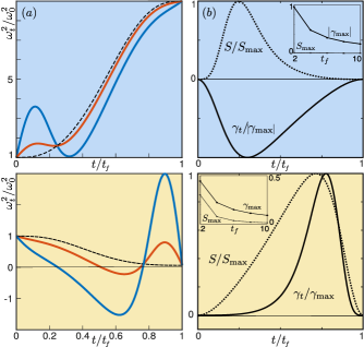
Figure 1: (a) Control frequency $\omega^{2}_{t}/\omega^{2}_{0}$ for protocols with duration $t_{f}=2$ (blue) and 6 (red), and reference frequency $\tilde{\omega}^{2}_{t}/\omega^{2}_{0}$ (dashed black). Fast protocols can require an inversion of the trap. (b) Dissipation rate $\gamma_{t}/\gamma_{\rm max}$ (solid lines) used to control the dynamics and relative entropy $S(\rho_{t}\|\sigma_{t})/S_{\rm max}$ (Eq. (20), dotted lines), showing the distance of the state to a reference thermal state. The shape of the dephasing strength and the relative entropy is independent on the duration of the protocol, which only influences their maxima. Protocols correspond to cooling, $\beta_{f}/\beta_{0}=2$, with compression (top, $\omega_{f}/\omega_{0}=3$) or expansion (bottom, $\omega_{f}/\omega_{0}=1/4$), with $\omega_{0}=\beta_{0}=1$.

Our scheme can be implemented by choosing an interpolating Ansatz between the boundary conditions imposed on the state, i.e. $\omega_{0/f}$ and $\beta_{0/f}$ that define $A_{0/f}$ and $C_{0/f}$. For illustration, we choose

$$A_{t} =A_{0}+(A_{f}-A_{0})\,f(t/t_{f}){\rm\,and}$$ (19a)

$$C_{t} =C_{0}+(C_{f}-C_{0})\,f(t/t_{f})$$ (19b)

in the form of a fifth-order polynomial, $f(\tau)=10\tau^{3}-15\tau^{4}+6\tau^{5}$, to ensure a smooth dynamics. The modulation of the control parameters $\omega_{t}^{2}$ and $\gamma_{t}$ readily follow from Eqs. (14-18). Fig. 1 illustrates the control frequency and dephasing strength corresponding to phase-space compression and expansion protocols, discussed below. Short control processes require trap inversion (a negative squared frequency), which can be achieved experimentally via, e.g., a painted potential Henderson et al. (2009) or a digital micromirror device Gauthier et al. (2016). They also rely on a dephasing strength of larger amplitude, which can be experimentally more challenging to achieve. We propose to use the maximum of the dephasing strength, denoted $\gamma_{\rm{max}}$ as a measure of the “cost” to implement the process by a technique such as stochastic parametric driving. We show in App. D that the maximum dephasing strength scales inversely with the process time, as illustrated in the insets of Fig. 1b.

We further use the relative entropy, defined as $S(\rho_{t}\|\sigma_{t})=\mathrm{Tr}\big{(}\rho_{t}\ln\rho_{t}\big{)}-\mathrm{Tr}\big{(}\rho_{t}\ln\sigma_{t}\big{)}$, as a measure of the distance of the engineered state $\rho_{t}$ to the effective thermal state $\sigma_{t}$ along the dynamics. It can be written as

$$S(\rho_{t}\|\sigma_{t})=\sum_{n=0}^{\infty}p_{n}\ln p_{n}-\sum_{m=0}^{\infty}(p_{n}\ln p_{m})\big{|}\langle m_{t}|n_{t}\rangle\big{|}^{2},$$ (20)

where the overlap of the eigenfunctions $\langle m_{t}|n_{t}\rangle$ is given explicitly in App. E following del Campo et al. (2017); Chenu et al. (2019); Andrews et al. (2000). Fig. 1 illustrates the relative entropy between the engineered and the thermal state. The insets show the maximum relative entropy for different process times, evidencing that the state is going further away from a thermal distribution for shorter protocols. The shape of the dephasing strength and the relative entropy is independent on the duration of the process, which only influences their maxima, $\gamma_{\rm max}$ and $s_{\rm max}$, respectively, as illustrated in Fig. 1b.

Figure 2: (a) Schematic representation of the phase-space map of final thermal states ($\beta_{f},\omega_{f}$) reachable from an initial thermal state ($\beta_{0}$, $\omega_{0}$), highlighted with the black dot, through STA control processes. States for which $\beta_{f}\omega_{f}=\beta_{0}\omega_{0}$, chosen along the gray line, can be obtained from unitary, phase-space preserving processes, with no entropy change. STA in open processes allow preparing arbitrary thermal states, while stochastic driving with $\gamma_{t}>0$ gives access to states for which $\beta_{f}\omega_{f}<\beta_{0}\omega_{0}$ (region highlighted in orange). (b) Associated change of the von Neumann entropy for $\omega_{0}=\beta_{0}=1$.

Superadiabatic protocols.— Processes satisfying $\beta_{f}\omega_{f}=\beta_{0}\omega_{0}$ conserve the mean phonon number and are often referred to as phase-space (density) preserving. The inverse temperature and frequency can be related to two physical lengths, namely, the particle characteristic length, given by the de Broglie wavelength, ${\it l}_{\rm{dB}}=\hbar\sqrt{\beta/(2m)}$, and the trap characteristic length, $\lambda_{{}_{\rm HO}}=\sqrt{\hbar/(m\omega)}$. Their ratio $l_{\rm{dB}}/{\lambda_{\rm HO}}=\sqrt{\beta\hbar\omega/2}$ is conserved for phase-space preserving transformation. STA in closed systems are limited to phase-space preserving cooling techniques, such as adiabatic cooling. These processes preserve the von Neumann entropy $S_{t}=-\rm{Tr}(\rho_{t}\ln\rho_{t})$ . By contrast, cooling and heating processes altering the phase-space density and the number of populated states lead to an entropy change Ketterle and Pritchard (1992) and require an open dynamics.

Figure 3: Maximum dephasing strength $\gamma_{\rm{max}}$: (a) Contour plot for an initial state $\beta_{0}=1=\omega_{0}$. We verify that $\gamma_{\rm{max}}$ is negative for $\beta_{f}\omega_{f}>\beta_{0}\omega_{0}$, and nonnegative otherwise; (b) as function of $\omega_{f}$ for fixed $\beta_{f}=1$; (c) as function of $\beta_{f}$, keeping the trap frequency unchanged ($\omega_{f}=1$), showing a plateau for large values of $\beta_{f}$; (d) and on a line of constant $\beta_{f}\omega_{f}=0.5$ showing that $\gamma_{\rm{max}}$ depends on the specific choice of $\beta_{f}$ and $\omega_{f}$.

STA for open processes thus allow reaching arbitrary thermal states ($\omega_{f}$, $\beta_{f})$ from an initial thermal state, as schematically represented in Fig. 2, along with the variation of entropy. The sign of the dephasing strength determines the variation of relative energy ${\rm sign}(\dot{\tilde{\varepsilon_{t}}})$ and entropy change. In particular, a positive dephasing strength yields a monotonic increase of entropy. Indeed, the rate of change of the von Neumann entropy reads

$$\frac{dS_{t}}{dt}=-\frac{\dot{u}_{t}}{(1-u_{t})^{2}}\ln(u_{t})=\gamma_{t}\frac{\varepsilon_{t}}{k_{t}^{2}}.$$ (21)

Protocols restricted to $\gamma_{t}\geq 0$ allow only STA for thermalization to high-temperature states (heating), with $\Delta S=S_{f}-S_{0}>0$. Whenever values of $\gamma_{t}$ can be engineered, this restriction is lifted.

The maximum dephasing strength, illustrated in Fig. 3, is specific to each scenario. It follows a different behavior when changing the trap frequency at constant temperature or vice versa. This is not surprising since the two parameters correspond to different physical phenomena, as discussed above. The plateau observed when decreasing the temperature at a fixed trap frequency (Fig. 3c) might be set by the trap size, which constrains the size of the particle. Interestingly, a given final phase-space density can be reached from different dephasing strengths, even when starting from a same initial state. In other words, processes yielding to $\beta_{f}\omega_{f}$ from $\beta_{0}\omega_{0}$ can have different implementation costs according to $\gamma_{\rm{max}}$, as illustrated in Fig. 3d.

In conclusion, we have introduced shortcuts to adiabaticity with an open dynamics engineered to control the thermalization of a quantum oscillator. The resulting protocols are expected to be broadly applicable as their implementation requires only a time modulation of the harmonic frequency and the dephasing strength, accessible e.g. via stochastic parametric driving or continuous quantum measurements. Our results can be directly applied to non-Markovian dynamics whenever the amplitude and sign of the dephasing strength can be engineered. Extension to obtain generalized Gibbs states and for interacting systems is under investigation.

Acknowledgments.— It is a pleasure to acknowledge discussions with Ángel Rivas and Bijay K. Agarwalla.

Appendix A Thermal state of a harmonic oscillator

It is well known that the thermal state of a harmonic oscillator is Gaussian in the coordinate representation. For the sake of completeness, we briefly sketch the derivation below. For a time-independent harmonic oscillator, the Hamiltonian $\hat{H}=\frac{\hat{p}^{2}}{2m}+\frac{1}{2}m\omega^{2}\hat{x}^{2}$ reads, in second quantization $\hbar\omega(a^{\dagger}a+\frac{1}{2})$, where $a=\sqrt{m\omega/2\hbar}\hat{x}+i\sqrt{1/2m\hbar\omega}\hat{p}$ is the annihilation operator. The coordinate representation of the thermal operator $e^{-\beta\hat{H}}/Z$ is easily written using the Fock states, defined as $a|n\rangle=\sqrt{n}|n-1\rangle$, and reads

$$\rho(x,x^{\prime})=\langle x|\frac{e^{-\beta\hat{H}}}{Z}|x^{\prime}\rangle=\frac{1}{Z}e^{-\beta\hbar\omega/2}\sum_{n}e^{-\beta\hbar\omega n}\langle x|n\rangle\langle n|x^{\prime}\rangle.$$ (22)

Solving the Schrödinger equation for the Fock state wave function $\langle x|n\rangle$ gives

$$\langle x|n\rangle=\sqrt{\frac{k}{2^{n}n!\sqrt{\pi}}}e^{-\frac{1}{2}(kx)^{2}}{H}_{n}\left(kx\right),$$ (23)

where $k^{-1}=\sqrt{\hbar/(m\omega)}$ denotes an effective length characteristic of the harmonic oscillator. The coordinate representation of the thermal density operator then reads

$$\rho(x,x^{\prime})=\frac{k}{Z\sqrt{\pi}}e^{-\beta\hbar\omega/2}\exp\left({-\frac{k^{2}}{2}(x^{2}+x^{\prime 2})}\right)\sum_{n}\left(\frac{e^{-\beta\hbar\omega}}{2}\right)^{n}\frac{1}{n!}{H}_{n}(kx){H}_{n}(kx^{\prime}).$$ (24)

We use Mehler’s formula Mehler (1866),

$$\sum_{n=0}^{\infty}\frac{u^{n}}{2^{n}n!}{H}_{n}(x){H}_{n}(y)=\frac{1}{\sqrt{1-u^{2}}}e^{2uxy/(1-u^{2})}e^{-u^{2}(x^{2}+y^{2})/(1-u^{2})},$$ (25)

to rewrite the sum with the Hermite polynomials as a Gaussian, yielding

$$\rho(x,x^{\prime})=\frac{k\sqrt{u}}{Z\sqrt{\pi}}\exp\left({-(k^{2}/2)(x^{2}+x^{\prime 2})}\right)\frac{1}{\sqrt{1-u^{2}}}\exp\left(-\frac{k^{2}}{(1-u^{2})}(u^{2}(x^{2}+x^{\prime 2})-2uxx^{\prime})\right),$$ (26)

where we have defined $u=e^{-\beta\hbar\omega}$. Finally, with the explicit form of the partition function $Z={\rm Tr}(e^{-\beta\hat{H}})=1/(1-u)$, this coordinate representation also takes the form

$$\rho(x,x^{\prime})=\frac{k}{\sqrt{\pi}}\sqrt{\tanh(\beta\hbar\omega/2)}\exp\left(-(k^{2}/2)\coth(\beta\hbar\omega)(x^{2}+x^{\prime 2})+k^{2}\sinh^{-1}(\beta\hbar\omega)xx^{\prime}\right).$$ (27)

The same derivation holds for a time dependent Hamiltonian, and provides the initial and final coefficients $A$ and $C$ given in the main text. We verify that the normalization factor is $\frac{k}{\sqrt{\pi}}\sqrt{\tanh(\beta\hbar\omega/2)}=\frac{k}{\sqrt{\pi}}\sqrt{\frac{1-u}{1+u}}=\sqrt{2(A+C)/\pi}$.

Appendix B Consistency equations from the evolution of the Gaussian Ansatz

The master equation (2) in the coordinate representation reads

$$\frac{d\rho_{t}(x,x^{\prime})}{dt}=\left(\frac{i\hbar}{2m}\Big{(}\frac{\partial^{2}}{\partial x^{2}}-\frac{\partial^{2}}{\partial x^{\prime 2}}\Big{)}-i\frac{m\omega_{t}^{2}}{2\hbar}(x^{2}-x^{\prime 2})-\gamma_{t}(x-x^{\prime})^{2}\right)\rho_{t}(x,x^{\prime}).$$ (28)

For the Gaussian Ansatz given in Eq. (3) of the main text, the real and imaginary parts of the evolution equation respectively give

$$\frac{\dot{N}_{t}}{N_{t}}+\frac{2\hbar}{m}B_{t} = \left(\dot{A}_{t}+\frac{4\hbar}{m}A_{t}B_{t}-\gamma_{t}\right)(x^{2}+x^{\prime 2})+2\left(\dot{C}_{t}+\frac{4\hbar}{m}B_{t}C_{t}+\gamma_{t}\right)xx^{\prime},$$ (29)

$$\dot{B}_{t} = \frac{2\hbar}{m}(A_{t}^{2}-B_{t}^{2}-C_{t}^{2})-\frac{m\omega_{t}^{2}}{2\hbar},$$ (30)

from which the consistency equations (4) directly follow.

Appendix C Instantaneous diagonalization of the density matrix

We look for the eigenvalues $p_{n,t}$ and eigenfunctions $|\psi_{n,t}\rangle$ that diagonalize the density matrix $\rho_{t}$ at any time. For the sake of simplicity, we omit the time dependence in the notation below. By definition, the eigenvalues fulfil $p_{n}>0$ and $\sum_{n}p_{n}=1$, so we choose to write them as $p_{n}=u^{n}(1-u)$, where $u$ can be seen as an exponential $e^{-\tilde{\varepsilon}}$. We verify below that the functions

$$\langle x|\psi_{n}\rangle=\sqrt{\frac{{k}}{2^{n}n!\sqrt{\pi}}}e^{-\frac{{k}^{2}}{2}x^{2}}e^{iBx^{2}}{H}_{n}({k}x)$$ (31)

correspond to the eigenfunctions. Note that orthogonality of the Hermite polynomials, $\int_{\infty}dx^{\prime}{H}_{n}({k}x^{\prime}){H}_{m}({k}x^{\prime})e^{-{k}x^{\prime 2}}=\delta_{nm}2^{n}n!\sqrt{\pi}/{k}$, guarantees orthonormality of the wave functions, $\langle\psi_{n}|\psi_{m}\rangle=\delta_{nm}$. To justify the choice of this Ansatz and determine the time-dependent variables ${k}$ and $u$, we start with the coordinate representation

$$\langle x|\rho_{t}|x^{\prime}\rangle=\sum_{n}u^{n}(1-u)\langle x|\psi_{n}\rangle\langle\psi_{n}|x^{\prime}\rangle,$$ (32)

and use Mehler’s equation (25) to get

$$\langle x|\rho_{t}|x^{\prime}\rangle=\frac{{k}}{\sqrt{\pi}}\sqrt{\frac{1-u}{1+u}}e^{-{k}^{2}(x^{2}+x^{\prime 2})(\frac{1}{2}+\frac{u^{2}}{1-u^{2}})}e^{iB(x^{2}-x^{\prime 2})}e^{\frac{2u{k}^{2}}{1-u^{2}}xx^{\prime}}.$$ (33)

By identification, we obtain

$$A={k}^{2}\frac{1+u^{2}}{2(1-u^{2})}=\frac{{k}^{2}}{2}\coth\tilde{\varepsilon},\qquad C=-{k}^{2}\frac{u}{1-u^{2}}=-\frac{{k}^{2}}{2\sinh\tilde{\varepsilon}},$$ (34)

the reverse transformation corresponding to the physical setting being for $u>0$ and $0<-A/C<1$, and

$${k}=\Big{(}2\sqrt{A^{2}-C^{2}}\Big{)}^{1/2},\qquad u=-\frac{A}{C}-\sqrt{\Big{(}\frac{A}{C}\Big{)}^{2}-1}.$$ (35)

The mean phonon number easily follows as $\langle n\rangle=\sum_{n=0}^{\infty}np_{n}=\frac{u}{1-u}$, and the von Neumann entropy $S(\rho)=-\rm{Tr}(\rho\log\rho)$ reads

$$S(\rho)=-\sum_{n=0}^{\infty}p_{n}\ln p_{n}=-\frac{u\ln u}{1-u}-\ln(1-u)\,.$$ (36)

Appendix D Maximum dephasing strength

We can show that the dephasing strength is inversely proportional to the time of the protocol for any polynomial Ansatz interpolating between the initial and final state. The time for which the dephasing strength is maximal is given from $\dot{\gamma}_{t_{\rm max}}=0$, which leads

$$\left.\frac{d^{2}f_{\tau}}{d^{2}\tau}\right|_{t_{\rm max}}=\left(\left.\frac{df_{\tau}}{d\tau}\right|_{t_{\rm max}}\right)^{2}(A_{f}-A_{0}+C_{f}-C_{0}),$$ (37)

where $\tau=t/t_{f}$ and where we have used $df_{\tau}/dt=df_{\tau}/d\tau(1/t_{f})$. This equation could be solved for a specific polynomial Ansatz $f_{\tau}=\sum_{n=0}^{N}f_{n}\tau^{n}$. Since $\gamma$ takes a zero value at initial and final time, a non-trivial solution goes through an extremum in the region $\tau\in[0:1]$. We denote the root corresponding to this time $r_{1}$. The maximum dephasing strength is reached at time $t_{max}=r_{1}t_{f}$. We further have

$$\gamma_{\rm max}=\frac{1}{t_{f}}\left.\frac{df_{\tau}}{d\tau}\right|_{t_{\rm max}}\frac{(A_{f}-A_{0})C_{t_{\rm max}}-A_{t_{\rm max}}(C_{f}-C_{0})}{A_{t_{\rm max}}+C_{t_{\rm max}}}.$$ (38)

The parameters $A_{t_{\rm max}}$ and $C_{t_{\rm max}}$ are polynomials of $r_{1}$ and all terms on the r.h.s, apart from $1/t_{f}$, depend only on the root $r_{1}$. This yields $\gamma_{\rm max}\propto 1/t_{f}$.

Appendix E Determine the eigenfunctions overlap in Eq. (20) to evaluate the relative entropy

We provide below the explicit form for the overlap

$$\langle m|n\rangle=\int_{-\infty}^{\infty}dx\langle m|x\rangle\langle x|n\rangle=\frac{{k}}{\sqrt{2^{n+m}n!m!\pi}}\int_{-\infty}^{\infty}dxe^{-{k}^{2}x^{2}}e^{-iBx^{2}}H_{m}\big{(}{k}x\big{)}H_{n}({k}x).$$

This overlap can be expressed as

$$\langle m|n\rangle=\frac{1}{\sqrt{2^{n+m}n!m!\pi}}I_{n,m}\left(1+iB/{k}^{2}\right)$$ (39)

by defining the integral

$$I_{n,m}(b)=\int_{-\infty}^{\infty}dx\,e^{-bx^{2}}{H}_{n}(x){H}_{m}(x),$$ (40)

where the indices $n$ and $m$ play a symmetric role. To solve this integral, we first write the exponential as $e^{-bx^{2}}=e^{-x^{2}}e^{-(b-1)x^{2}}$ in order to have a Gaussian for each Hermite polynomial. Then, multiple integration by parts yield $\int dx\,e^{-x^{2}}{H}_{n}(x)f(x)=\int dx\,e^{-x^{2}}D^{n}(g(x))$, where $D^{n}\equiv(d/dx)^{n}$, for any function $g(x)$ del Campo et al. (2017); Chenu et al. (2019). So, for $g(x)=e^{-(b-1)x^{2}}{H}_{m}(x)$, and choosing $n<m$ by convention, we find

$$I_{n,m}(b)=\int_{-\infty}^{\infty}dx\,e^{-x^{2}}D^{n}\big{(}e^{-(b-1)x^{2}}\big{)}{H}_{m}(x).$$ (41)

We then expand the derivative $D^{n}$ in a binomial form, use the derivative of the Hermite polynomial, $D^{j}({H}_{N}(x))=2^{j}N!/(N-j)!{H}_{N-j}(x)$, and the definition of the Hermite polynomial $e^{-x^{2}}{H}_{N}(x)=(-D)^{N}e^{-x^{2}}$ to obtain

$$I_{n,m}(b) = \sum_{l=0}^{n}\binom{n}{l}\frac{2^{n-l}m!}{(m-n+l)!}\int_{-\infty}^{\infty}dxe^{-x^{2}}D^{l}\big{(}e^{-(b-1)x^{2}}\big{)}{H}_{m-n+l}(x)$$ (42)

$$= \sum_{l=0}^{n}\binom{n}{l}\frac{2^{n-l}m!(-1)^{m-n+l}}{(m-n+l)!}\int_{-\infty}^{\infty}dxD^{l}\big{(}e^{-(b-1)x^{2}}\big{)}D^{m-n+l}\big{(}e^{-x^{2}}\big{)}.$$

In order to evaluate the new integral, we write each of the derivates as a Fourier transform, using $D^{n}(e^{-x^{2}})=(2i)^{n}/\sqrt{\pi}\int_{\infty}dt\,e^{-t^{2}}tne^{2ixt}$ Andrews et al. (2000), which gives, taking $\alpha=(1-b)$ and $j=(m-n+l)$,

$$\int_{-\infty}^{\infty}dx\,D^{l}\big{(}e^{-\alpha x^{2}}\big{)}D^{j}\big{(}e^{-x^{2}}\big{)} = \frac{(2i)^{l+j}\sqrt{\alpha}^{l}}{\pi}\int_{-\infty}^{\infty}dtds\,e^{t^{2}+s^{2}}t^{l}s^{l}\int_{-\infty}^{\infty}dx\,e^{2ix(\sqrt{\alpha}t+s)}$$ (43)

$$= (-1)^{j}(2i\sqrt{\alpha})^{l+j}\int_{-\infty}^{\infty}dt\,e^{-t^{2}(1+\alpha)}t^{l+j}$$

$$= (-1)^{j}(2i\sqrt{\alpha})^{l+j}\frac{1}{2}(1+\alpha)^{-\frac{l+j+1}{2}}(1+(-1)^{l+j})\Gamma\big{(}\frac{l+j+1}{2}\big{)}.$$

This leads to

$$I_{n,m}(b)=(1+(-1)^{m-n})\sum_{l=0}^{n}2^{m+l-1}\binom{n}{l}\frac{m!}{(m-n+l)!}i^{m-n+2l}\left(1-\frac{1}{b}\right)^{\frac{2l+m-n}{2}}\frac{1}{\sqrt{b}}\>\Gamma\left(\frac{1+m-n}{2}+l\right).$$ (44)

We can further simplify this expression by noting that it is non-zero only for $(l+j)=(m-n+2l)$ even. Choosing $m>n$ by convention, we thus find $I_{n,n+2p+1}=0$ for all integers $p$, and

$$I_{n,n+2p}(b)=\sqrt{\frac{\pi}{b}}\sum_{l=0}^{n}\binom{n}{l}2^{n-l}\left(\frac{1-b}{b}\right)^{p+l}\frac{(2p+n)!(2p+2l)!}{(2p+l)!(l+p)!},$$ (45)

where we have used $\Gamma(1/2+n)=\sqrt{\pi}(2n)!/(4^{n}n!)$ to explicitly write the Gamma function from Eq. (43). Note that this sum can also be written using the hypergeometric function ${}_{2}F_{1}$, specifically

$$I_{n,n+2p}(b)=2^{n}\sqrt{\frac{\pi}{b}}\left(\frac{1-b}{b}\right)^{p}\frac{(2p+n)!}{p!}{}_{2}F_{1}\left(\frac{1}{2}+p,-n,1+2p,2-\frac{2}{b}\right).$$ (46)

Using this expression or Eq. (45) in (39) with $b=1+iB/{k^{2}}$ yields the overlap of interest.

References

- Torrontegui et al. (2013) Erik Torrontegui, Sara Ibáñez, Sofia Martínez-Garaot, Michele Modugno, Adolfo del Campo, David Guéry-Odelin, Andreas Ruschhaupt, Xi Chen, and Juan Gonzalo Muga, “Chapter 2 - shortcuts to adiabaticity,” in Advances in Atomic, Molecular, and Optical Physics, Advances In Atomic, Molecular, and Optical Physics, Vol. 62, edited by Ennio Arimondo, Paul R. Berman, and Chun C. Lin (Academic Press, 2013) pp. 117 – 169.
- Schaff et al. (2010) J.-F. Schaff, X.-L. Song, P. Vignolo, and G. Labeyrie, “Fast optimal transition between two equilibrium states,” Phys. Rev. A 82, 033430 (2010).
- Schaff et al. (2011) J.-F. Schaff, X.-L. Song, P. Capuzzi, P. Vignolo, and G. Labeyrie, “Shortcut to adiabaticity for an interacting bose-einstein condensate,” EPL (Europhysics Letters) 93, 23001 (2011).
- Bason et al. (2012) M. G. Bason, M. Viteau, N. Malossi, P. Huillery, E. Arimondo, R. Fazio, V. Giovannetti, R. Mannella, and O. Morsch, “High-fidelity quantum driving,” Nature Physics 8, 147 (2012).
- Rohringer et al. (2015) W. Rohringer, D. Fischer, F. Steiner, J. Mazets, I. E. afnd Schmiedmayer, and M. Trupke, “Non-equilibrium scale invariance and shortcuts to adiabaticity in a one-dimensional bose gas,” Sci. Rep. 5, 9820 (2015).
- Deng et al. (2018a) Shujin Deng, Pengpeng Diao, Qianli Yu, Adolfo del Campo, and Haibin Wu, “Shortcuts to adiabaticity in the strongly coupled regime: Nonadiabatic control of a unitary fermi gas,” Phys. Rev. A 97, 013628 (2018a).
- Deng et al. (2018b) Shujin Deng, Aurélia Chenu, Pengpeng Diao, Fang Li, Shi Yu, Ivan Coulamy, Adolfo del Campo, and Haibin Wu, “Superadiabatic quantum friction suppression in finite-time thermodynamics,” Science Advances 4, eaar5909 (2018b).
- Du et al. (2016) Yan-Xiong Du, Zhen-Tao Liang, Yi-Chao Li, Xian-Xian Yue, Qing-Xian Lv, Wei Huang, Xi Chen, Hui Yan, and Shi-Liang Zhu, “Experimental realization of stimulated raman shortcut-to-adiabatic passage with cold atoms,” Nature communications 7, 12479 (2016).
- An et al. (2016) Shuoming An, Dingshun Lv, Adolfo del Campo, and Kihwan Kim, “Shortcuts to adiabaticity by counterdiabatic driving for trapped-ion displacement in phase space,” Nature Communications 7, 1–5 (2016).
- Zhang et al. (2013) Jingfu Zhang, Jeong Hyun Shim, Ingo Niemeyer, T. Taniguchi, T. Teraji, H. Abe, S. Onoda, T. Yamamoto, T. Ohshima, J. Isoya, and Dieter Suter, “Experimental implementation of assisted quantum adiabatic passage in a single spin,” Phys. Rev. Lett. 110, 240501 (2013).
- Wang et al. (2018) Tenghui Wang, Zhenxing Zhang, Liang Xiang, Zhilong Jia, Peng Duan, Weizhou Cai, Zhihao Gong, Zhiwen Zong, Mengmeng Wu, Jianlan Wu, Luyan Sun, Yi Yin, and Guoping Guo, “The experimental realization of high-fidelity ‘shortcut-to-adiabaticity’ quantum gates in a superconducting xmon qubit,” New Journal of Physics 20, 065003 (2018).
- Zhang et al. (2018) Zhenxing Zhang, Tenghui Wang, Liang Xiang, Zhilong Jia, Peng Duan, Weizhou Cai, Ze Zhan, Zhiwen Zong, Jianlan Wu, Luyan Sun, Yi Yin, and Guoping Guo, “Experimental demonstration of work fluctuations along a shortcut to adiabaticity with a superconducting xmon qubit,” New Journal of Physics 20, 085001 (2018).
- Jarzynski (2013) Christopher Jarzynski, “Generating shortcuts to adiabaticity in quantum and classical dynamics,” Phys. Rev. A 88, 040101 (2013).
- Deffner et al. (2014) Sebastian Deffner, Christopher Jarzynski, and Adolfo del Campo, “Classical and quantum shortcuts to adiabaticity for scale-invariant driving,” Phys. Rev. X 4, 021013 (2014).
- Schmiedl and Seifert (2007) Tim Schmiedl and Udo Seifert, “Optimal finite-time processes in stochastic thermodynamics,” Phys. Rev. Lett. 98, 108301 (2007).
- Demirplak and Rice (2003) Mustafa Demirplak and Stuart A Rice, “Adiabatic population transfer with control fields,” J. Phys. Chem. A 107, 9937 (2003).
- Demirplak and Rice (2005) Mustafa Demirplak and Stuart A Rice, “Assisted adiabatic passage revisited,” J. Phys. Chem. B 109, 6838 (2005).
- Berry (2009) M V Berry, “Transitionless quantum driving,” Journal of Physics A: Mathematical and Theoretical 42, 365303 (2009).
- Masuda and Nakamura (2009) S. Masuda and K. Nakamura, “Fast-forward of adiabatic dynamics in quantum mechanics,” Proc. R. Soc. London Ser. A 466, 1135 (2009).
- Masuda et al. (2014) Shumpei Masuda, Katsuhiro Nakamura, and Adolfo del Campo, “High-fidelity rapid ground-state loading of an ultracold gas into an optical lattice,” Phys. Rev. Lett. 113, 063003 (2014).
- Chen et al. (2010) Xi Chen, A. Ruschhaupt, S. Schmidt, A. del Campo, D. Guéry-Odelin, and J. G. Muga, “Fast optimal frictionless atom cooling in harmonic traps: Shortcut to adiabaticity,” Phys. Rev. Lett. 104, 063002 (2010).
- Muga et al. (2009) J G Muga, Xi Chen, A Ruschhaupt, and D Guéry-Odelin, “Frictionless dynamics of Bose-Einstein condensates under fast trap variations,” Journal of Physics B: Atomic, Molecular and Optical Physics 42, 241001 (2009).
- del Campo (2011) A. del Campo, “Frictionless quantum quenches in ultracold gases: A quantum-dynamical microscope,” Phys. Rev. A 84, 031606 (2011).
- del Campo (2013) Adolfo del Campo, “Shortcuts to adiabaticity by counterdiabatic driving,” Phys. Rev. Lett. 111, 100502 (2013).
- Okuyama and Takahashi (2016) Manaka Okuyama and Kazutaka Takahashi, “From classical nonlinear integrable systems to quantum shortcuts to adiabaticity,” Phys. Rev. Lett. 117, 070401 (2016).
- Sels and Polkovnikov (2017) D. Sels and A. Polkovnikov, “Minimizing irreversible losses in quantum systems by local counterdiabatic driving,” Proceedings of the National Academy of Sciences 114, E3909 (2017).
- Claeys et al. (2019) Pieter W. Claeys, Mohit Pandey, Dries Sels, and Anatoli Polkovnikov, “Floquet-engineering counterdiabatic protocols in quantum many-body systems,” Phys. Rev. Lett. 123, 090602 (2019).
- Calzetta (2018) Esteban Calzetta, “Not-quite-free shortcuts to adiabaticity,” Phys. Rev. A 98, 032107 (2018).
- Levy et al. (2018) Amikam Levy, A Kiely, J G Muga, R Kosloff, and E Torrontegui, “Noise resistant quantum control using dynamical invariants,” New Journal of Physics 20, 025006 (2018).
- Feldmann and Kosloff (2006) Tova Feldmann and Ronnie Kosloff, “Quantum lubrication: Suppression of friction in a first-principles four-stroke heat engine,” Phys. Rev. E 73, 025107 (2006).
- Deng et al. (2013) Jiawen Deng, Qing-hai Wang, Zhihao Liu, Peter Hänggi, and Jiangbin Gong, “Boosting work characteristics and overall heat-engine performance via shortcuts to adiabaticity: Quantum and classical systems,” Phys. Rev. E 88, 062122 (2013).
- del Campo et al. (2014) Adolfo del Campo, J Goold, and M Paternostro, “More bang for your buck: Super-adiabatic quantum engines,” Sci. Rep. 4 (2014), 10.1038/srep06208.
- Beau et al. (2016) Mathieu Beau, Juan Jaramillo, and Adolfo del Campo, “Scaling-up quantum heat engines efficiently via shortcuts to adiabaticity,” Entropy 18, 168 (2016).
- Villazon et al. (2019) Tamiro Villazon, Anatoli Polkovnikov, and Anushya Chandran, “Swift heat transfer by fast-forward driving in open quantum systems,” Phys. Rev. A 100, 012126 (2019).
- Dann and Kosloff (2019) Roie Dann and Ronnie Kosloff, “Quantum Signatures in the Quantum Carnot Cycle,” arXiv e-prints , arXiv:1906.06946 (2019), arXiv:1906.06946 [quant-ph] .
- Vacanti et al. (2014) G Vacanti, R Fazio, S Montangero, G M Palma, M Paternostro, and V Vedral, “Transitionless quantum driving in open quantum systems,” New Journal of Physics 16, 053017 (2014).
- Duncan and del Campo (2018) Callum W Duncan and Adolfo del Campo, “Shortcuts to adiabaticity assisted by counterdiabatic born–oppenheimer dynamics,” New Journal of Physics 20, 085003 (2018).
- Dann et al. (2019) Roie Dann, Ander Tobalina, and Ronnie Kosloff, “Shortcut to equilibration of an open quantum system,” Phys. Rev. Lett. 122, 250402 (2019).
- Alipour et al. (2019) S. Alipour, A Chenu, A. T. Rezakhani, and A. del Campo, “Shortcuts to Adiabaticity in Driven Open Quantum Systems: Balanced Gain and Loss and Non-Markovian Evolution,” arXiv e-prints , arXiv:1907.07460 (2019), arXiv:1907.07460 [quant-ph] .
- Rivas et al. (2014) Ángel Rivas, Susana F Huelga, and Martin B Plenio, “Quantum non-markovianity: characterization, quantification and detection,” Reports on Progress in Physics 77, 094001 (2014).
- Budini (2001) Adrián A. Budini, “Quantum systems subject to the action of classical stochastic fields,” Phys. Rev. A 64, 052110 (2001).
- Chenu et al. (2017) A. Chenu, M. Beau, J. Cao, and A. del Campo, “Quantum simulation of generic many-body open system dynamics using classical noise,” Phys. Rev. Lett. 118, 140403 (2017).
- Smith et al. (2018) Andrew Smith, Yao Lu, Shuoming An, Xiang Zhang, Jing-Ning Zhang, Zongping Gong, H T Quan, Christopher Jarzynski, and Kihwan Kim, “Verification of the quantum nonequilibrium work relation in the presence of decoherence,” New Journal of Physics 20, 013008 (2018).
- Korotkov (1999) Alexander N. Korotkov, “Continuous quantum measurement of a double dot,” Phys. Rev. B 60, 5737–5742 (1999).
- Carmichael (2013) Howard J Carmichael, Statistical methods in quantum optics 1: master equations and Fokker-Planck equations (Springer Science & Business Media, 2013).
- Adler (2003) Stephen L. Adler, “Weisskopf-Wigner decay theory for the energy-driven stochastic Schrödinger equation,” Phys. Rev. D 67, 025007 (2003).
- Gardiner (2009) C. Gardiner, Stochastic Methods: A Handbook for the Natural and Social Sciences, Springer Series in Synergetics (Springer Berlin Heidelberg, 2009).
- Ruschhaupt et al. (2012) A Ruschhaupt, Xi Chen, D Alonso, and J G Muga, “Optimally robust shortcuts to population inversion in two-level quantum systems,” New J. Phys. 14, 093040 (2012).
- Jacobs and Steck (2006) Kurt Jacobs and Daniel A. Steck, “A straightforward introduction to continuous quantum measurement,” Contemporary Physics 47, 279–303 (2006).
- Wiseman and Milburn (2009) Howard M. Wiseman and Gerard J. Milburn, Quantum Measurement and Control (Cambridge University Press, 2009).
- Jacobs (2014) Kurt Jacobs, Quantum Measurement Theory and its Applications (Cambridge University Press, 2014) chap. 3.
- Jacobs (2007) Kurt Jacobs, “Feedback control for communication with non-orthogonal states,” Quantum Info. Comput. 7, 127–138 (2007).
- Dann et al. (2018) Roie Dann, Amikam Levy, and Ronnie Kosloff, “Time-dependent markovian quantum master equation,” Phys. Rev. A 98, 052129 (2018).
- Leibfried et al. (2003) D. Leibfried, R. Blatt, C. Monroe, and D. Wineland, “Quantum dynamics of single trapped ions,” Rev. Mod. Phys. 75, 281–324 (2003).
- Myatt et al. (2000) C. Myatt, B. King, Q. A. Turchette, C.A. Sackett, D. Kielpinski, W.M. Itano, C. Monroe, and D. Wineland, “Decoherence of quantum superpositions through coupling to engineered reservoirs,” Nature 403, 269 (2000).
- Turchette et al. (2000) Q. A. Turchette, C. J. Myatt, B. E. King, C. A. Sackett, D. Kielpinski, W. M. Itano, C. Monroe, and D. J. Wineland, “Decoherence and decay of motional quantum states of a trapped atom coupled to engineered reservoirs,” Phys. Rev. A 62, 053807 (2000).
- Mehler (1866) F. G. Mehler, “Ueber die entwicklung einer function von beliebig vielen variabeln nach laplaceschen functionen höherer ordnung,” J. für die Reine und Angewandte Mathematik 66, 161 (1866), cf. p 174, eqn (18) & p 173, eqn (13).
- Henderson et al. (2009) K Henderson, C Ryu, C MacCormick, and M G Boshier, “Experimental demonstration of painting arbitrary and dynamic potentials for bose–einstein condensates,” New Journal of Physics 11, 043030 (2009).
- Gauthier et al. (2016) G. Gauthier, I. Lenton, N. McKay Parry, M. Baker, M. J. Davis, H. Rubinsztein-Dunlop, and T. W. Neely, “Direct imaging of a digital-micromirror device for configurable microscopic optical potentials,” Optica 3, 1136–1143 (2016).
- del Campo et al. (2017) A. del Campo, J. Molina-Vilaplana, and J. Sonner, “Scrambling the spectral form factor: Unitarity constraints and exact results,” Phys. Rev. D 95, 126008 (2017).
- Chenu et al. (2019) Aurélia Chenu, Javier Molina-Vilaplana, and Adolfo del Campo, “Work statistics, loschmidt echo and information scrambling in chaotic quantum systems,” Quantum 3, 127 (2019).
- Andrews et al. (2000) George E Andrews, Richard Askey, and Ranjan Roy, Special functions, Vol. 71 (Cambridge university press, 2000) eq. (6.1.2) p.278.
- Ketterle and Pritchard (1992) Wolfgang Ketterle and David E. Pritchard, “Atom cooling by time-dependent potentials,” Phys. Rev. A 46, 4051–4054 (1992).