Time-resolved spectrum output from a grating spectrometer

Abstract

Time-resolved spectra are often recorded in optical Thomson scattering experiments of laser-produced plasmas. In this essay, the meaning of time-resolved spectra output from a grating spectrometer is examined. Our results show that the recorded signal is indeed the convolution of the response function of dispersion element and the product of instant local dynamic form factor and electron density.

I Introduction

The Thomson scattering is a powerful diagnostics for plasma physics because it can provide accurate and reliable information of high temperature plasmas Froula et al. (2011). In the fields of high-energy-density physics in relevance to laser fusion and laboratory astrophysics, the Thomson scattering systems have been developed for various laser facilities Fontaine et al. (1994); Glenzer et al. (1997); Bai et al. (2001); Wang et al. (2005); Ross et al. (2006, 2011); Gong et al. (2015); Ross et al. (2016); Zhao et al. (2018). With novel schemes of experimental setup and data analysis Ross et al. (2011); Follett et al. (2016); Liu, Ding, and Zheng (2019), plasma parameters can be inferred with high accuracy, making Thomson scattering as key tool for quantitative study of high-energy-density physics. It becomes necessary that subtle effects must be included in the theory of Thomson scattering Zheng, Yu, and Zheng (1997); Myatt et al. (1998); Zheng, Yu, and Zheng (1999); Rozmus et al. (2000); Belyi (2002); Tierney et al. (2003); Zheng and Yu (2009); Palastro et al. (2010); Kozlowski et al. (2016); Rozmus et al. (2017); Belyi (2018). Many important physical processes have been experimentally investigated with this powerful technique Glenzer et al. (1996, 1999); Froula et al. (2007); Li et al. (2013); Rinderknecht et al. (2018); Henchen et al. (2018); Davies et al. (2019); Milder et al. (2020); Turnbull et al. (2020).

High-energy-density plasmas generated with high power laser pulses usually evolve rapidly with time because of great pressure gradient. In a modern experiment of optical Thomson scattering off laser-produced plasmas, scattered light waves are usually collected with an imaging system and are then relayed into a grating spectrometer coupled with a streak camera. With such kind of experimental setup, time-resolved Thomson scattering spectra are obtained, from which physical processes of interest are then inferred. However, to the best knowledge of the authors, the exact meaning of time-resolved spectrum obtained with above mentioned method is never clarified. Since Thomson scattering have been a very accuracy experiment tool for plasma physics, the meaning of the recorded signal should be carefully checked. In this article, we address this topic and discuss the relation between the recorded signal and the dynamic form factor.

II Output of a grating spectrometer

We assume that a point light source is incident onto a grating after collimated with an ideal lens. The diffracted light wave due to the grating is then focused with another lens onto the slit of a streak camera. Shown in Fig. 1 is the schematic setup, in which the incident angle is $\phi$ and the diffraction angle is $\theta$.

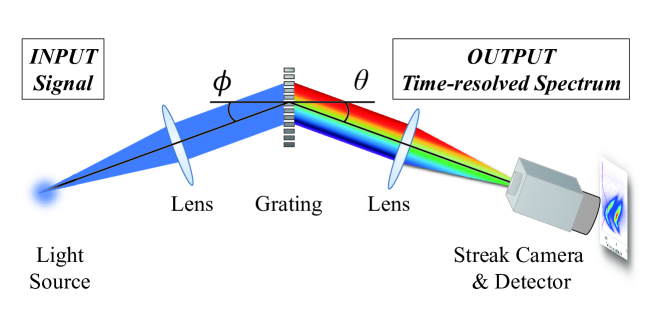
Figure 1: Schematic setup of time-resolved Thomson scattering measurement.

We describe the point source with a function $E(t)$. The output signal in the spectral plane of the spectrometer is given by

$$I(t,\theta)=\left|\frac{1}{N}\sum_{k=-N/2}^{N/2-1}E(t-k\tau_{\theta})\right|^{2},$$ (1)

where $\tau_{\theta}$ is time delay between two diffracted light waves from two adjacent groove lines of the grating,

$$\tau(\theta)=\frac{d}{c}(\sin\phi+\sin\theta).$$ (2)

Here $d$ is the grating constant, $c$ is the light speed, and $N$ is the total number of the active groove lines of the grating. The output signal depends on the time $t$ as well as the diffraction angle $\theta$ which determines the frequency through the Bragg equation. Therefore, Eq. (1) describes time-resolved spectrum.

With the introduction of the grating function $G$ defined as

$$G(t)=\frac{1}{N}\sum_{n=-N/2}^{N/2-1}\delta(t-n\tau_{\theta}),$$ (3)

the output signal (1) can be written as the square of the convolution of the input signal and the grating function,

$$I(t,\theta)=\left|\int_{-\infty}^{\infty}E(s)G(t-s)d\tau\right|^{2}.$$ (4)

It is straightforward to show that the right hand side of Eq. (4) can be described with two Wigner functions Diels and Rudolph (2006),

$$I(t,\theta)=\frac{1}{2\pi}\int_{-\infty}^{\infty}ds\int_{-\infty}^{\infty}d\omega W_{G}(t-s,\omega)W_{E}(s,\omega).$$ (5)

Here the Wigner function for a function $F$ is defined as

$$W_{F}(t,\omega)=\int_{-\infty}^{\infty}F^{\ast}(t-s/2)F(t+s/2)e^{-i\omega s}ds.$$ (6)

As seen in Eq. (5), the time-resolved spectrum is the convolution of two Wigner functions: one is from the instrument of known, the other is from the signal of interest.

Making the Fourier transformation of the Wigner functions with respect to the time variable,

$$\hat{I}(\chi,\theta) =\int_{-\infty}^{\infty}I(t,\theta)e^{-i\chi t}dt,$$

$$\hat{W}_{F}(\chi,\omega) =\int_{-\infty}^{\infty}W_{F}(t,\omega)e^{-i\chi t}dt,$$

Eq. (5) can be simplified in the frequency domain,

$$\hat{I}(\chi,\theta)=\int_{-\infty}^{\infty}\hat{W}_{G}(\chi,\omega)\hat{W}_{E}(\chi,\omega)\frac{d\omega}{2\pi}.$$ (7)

III Chirped pulse: an example

We are interested in the case that the frequency of the input signal is dependent of time. As an example, we first consider the experiment that a laser beam is scattered from a beam of uniformly accelerated electrons in non-relativistic condition. We assume that the laser pulse is a gaussian and that the velocity of the electron beam is given by

$$\mathbf{v}=\mathbf{a}t\text{ and }v\ll c.$$ (8)

Here $c$ is the light speed in vacuum. In this case, the scattering process can be approximated with the dipole radiation, and the signal can be described with the following equation,

$$E(t)=E_{0}e^{-\alpha t^{2}/2+i\omega_{0}t+i\beta t^{2}/2},$$ (9)

where $\omega_{0}$ is the frequency of the laser probe, $\alpha^{-1/2}$ is its pulse duration, and $\beta=\mathbf{k}\cdot\mathbf{a}$, and $\mathbf{k}$ is the differential wave number of the scattering. It is easy to show that the Wigner function of the input signal is then given by

$$W_{E}(t,\omega)=2E_{0}^{2}\sqrt{\frac{\pi}{\alpha}}e^{-\alpha t^{2}-(\omega-\omega_{0}-\beta t)^{2}/\alpha}.$$ (10)

Its Fourier component is

$$\hat{W}_{E}(\chi,\omega)=\frac{2\pi E_{0}^{2}}{\sqrt{\alpha^{2}+\beta^{2}}}e^{-\frac{\alpha\chi^{2}}{4(\alpha^{2}+\beta^{2})}-\frac{\alpha(\omega-\omega_{0})^{2}}{\alpha^{2}+\beta^{2}}-i\frac{\beta(\omega-\omega_{0})\chi}{\alpha^{2}+\beta^{2}}}$$ (11)

The Fourier component of the Wigner function $\hat{W}_{G}(\chi,\omega)$ for the grating can also be easily obtained,

$$\hat{W}_{G}(\chi,\omega)=e^{i\chi\tau_{\theta}}\mathcal{G}(\omega-\chi/2)\mathcal{G}(\omega+\chi/2),$$ (12)

where the function $\mathcal{G}(\omega)$ is defined as Born and Wolf (1999)

$$\mathcal{G}(\omega)=\frac{\sin(N\omega\tau_{\theta}/2)}{N\sin(\omega\tau_{\theta}/2)}.$$ (13)

In the case of $N\gg 1$, the function $\mathcal{G}(\omega)$ have a series of sharp spikes locating at

$$\omega\tau_{\theta}=2n\pi,\text{ where }n=0,\pm 1,\pm 2,\cdots.$$ (14)

For the sake of analytical calculation, we make the approximation

$$\mathcal{G}(\omega)\sim e^{-(\omega\tau_{\theta}-2\pi)/\sigma_{N}^{2}},\text{ where }\sigma_{N}=0.7\pi/N.$$ (15)

With this approximation, we have

$$\hat{W}_{G}(\chi,\omega)=e^{i\chi\tau_{\theta}-\frac{(\omega\tau_{\theta}-2\pi)^{2}}{\sigma_{N}^{2}}-\frac{\chi^{2}\tau_{\theta}^{2}}{4\sigma_{N}^{2}}}.$$ (16)

We introduce the diffraction angle shift $\Delta\theta$,

$$\Delta\theta=\theta-\theta_{0}.$$

where $\theta_{0}$ is defined as

$$\frac{d}{\lambda_{0}}(\sin\phi+\sin\theta_{0})=1,\text{ where }\lambda_{0}=\frac{2\pi c}{\omega_{0}}.$$

After some basic calculations, we obtain the time-resolved spectrum of the chirped pulse (9) output from a grating spectrometer,

$$I(t,\Delta\theta)=\frac{(\sigma_{N}/\tau_{0})^{2}E_{0}^{2}}{\sqrt{\beta^{2}+(\alpha+(\sigma_{N}/\tau_{0})^{2})^{2}}}e^{-(a\omega_{0})^{2}\frac{\alpha+(\sigma_{N}/\tau_{0})^{2}}{\beta^{2}+[a+(\sigma_{N}/\tau_{0})^{2}]^{2}}\left[\Delta\theta+\frac{\beta}{a\omega_{0}}\frac{(\sigma_{N}/\tau_{0})^{2}}{\alpha+(\sigma_{N}/\tau_{0})^{2}}t\right]^{2}-\frac{(\sigma_{N}/\tau_{0})^{2}\alpha t^{2}}{\alpha+(\sigma_{N}/\tau_{0})^{2}}},$$ (17)

were $a$ and $\tau_{0}$ are defined as

$$a=\frac{\cos\theta_{0}}{\sin\phi+\sin\theta_{0}},$$

and

$$\tau_{0}=\tau_{\theta}(\theta_{0}).$$

The result (17) shows that at any given time $t$ the output signal has a maximum locating at the diffraction angle

$$\Delta\theta=-\frac{\beta}{a\omega_{0}}\frac{(\sigma_{N}/\tau_{0})^{2}}{\alpha+(\sigma_{N}/\tau_{0})^{2}}t.$$

The measured frequency shift $\Delta\omega=\omega-\omega_{0}$, which can be found through the Bragg equation (14), depends on the diffraction angle $\Delta\theta$ through the following equation,

$$\Delta\omega=-a\omega_{0}\Delta\theta.$$ (18)

The time-resolve spectrum of a chirped pulse output from a grating spectrometer is

$$I(t,\Delta\omega)=\frac{(\sigma_{N}/\tau_{0})^{2}E_{0}^{2}}{\sqrt{\beta^{2}+(\alpha+(\sigma_{N}/\tau_{0})^{2})^{2}}}e^{-\frac{\alpha+(\sigma_{N}/\tau_{0})^{2}}{\beta^{2}+[a+(\sigma_{N}/\tau_{0})^{2}]^{2}}\left[\Delta\omega-\frac{(\sigma_{N}/\tau_{0})^{2}}{\alpha+(\sigma_{N}/\tau_{0})^{2}}\beta t\right]^{2}-\frac{(\sigma_{N}/\tau_{0})^{2}\alpha t^{2}}{\alpha+(\sigma_{N}/\tau_{0})^{2}}}.$$ (19)

As seen in Eq. (19), the measured frequency shift of the chirped pulse depends on time as

$$\Delta\omega=\frac{(\sigma/\tau_{0})^{2}}{\alpha+(\sigma/\tau_{0})^{2}}\beta t.$$

The changing rate of the measured frequency becomes smaller due to the dispersion of the grating. After integrating over the frequency $\Delta\omega$, we obtain the spectral-integrated signal,

$$I(t)\sim e^{-\frac{(\sigma_{N}/\tau_{0})^{2}\alpha t^{2}}{\alpha+(\sigma_{N}/\tau_{0})^{2}}}.$$

In comparison with the input signal, the output pulse becomes a little longer due to the dispersion of the grating. In the case of

$$\alpha\ll(\sigma_{N}/\tau_{0})^{2},$$

the effects of the grating on the frequency and duration of the chirped pulse becomes negligible,

$$I(t,\Delta\omega)=\frac{(\sigma_{N}/\tau_{0})^{2}E_{0}^{2}}{\sqrt{\beta^{2}+(\sigma_{N}/\tau_{0})^{4}}}e^{-\frac{(\sigma_{N}/\tau_{0})^{2}}{\beta^{2}+(\sigma_{N}/\tau_{0})^{4}}(\Delta\omega-\beta t)^{2}-\alpha t^{2}.}$$

IV Time-resovled spectrum of Thomson scattering

In an experiment of Thomson scattering off laser-produced plasmas, the observed scattering spectra usually vary with time due to the temporal evolutions of plasma parameters such as electron temperature and plasma flow velocity, etc. In the case that the incident wave is plane and monochromatic, the electric field of scattering waves from a plasma in non-relativistic case is given by Oberman and Williams (1983)

$$\mathbf{E}_{s}(\mathbf{R},t)=\frac{r_{e}\mathbf{n}\times(\mathbf{n}\times\mathbf{E}_{0})}{2R}\int_{V}d^{3}r\int d\tau\int\frac{d\omega_{s}}{2\pi}\left[e^{-i\omega_{s}(t-R/c)}e^{i(\omega_{s}-\omega_{0})\tau-i(\mathbf{n}\omega_{s}/c-\mathbf{k}_{0})\cdot\mathbf{r}}+\text{C.C.}\right]\hat{n}_{e}(\mathbf{r},\tau).$$ (20)

Here $\mathbf{R}$ is the position of the objective lens of the scattering system, $\mathbf{n}=\mathbf{R}/R$ is the scattering direction, $r_{e}$ is the classical electron radius, $(\omega_{0},\mathbf{k}_{0})$ are the frequency and wave vector of the incident light wave, $\mathbf{E}_{0}$ is the amplitude of the incident wave, C.C. denotes the complex conjugation term, and $\hat{n}_{e}(\mathbf{r},\tau)$ is the exact electron density defined as

$$\hat{n}_{e}(\mathbf{r},\tau)=\sum_{j=1}^{N_{e}}\delta(\mathbf{r}-\mathbf{r}_{j}(\tau)).$$ (21)

The time-dependent part of the scattering wave field can be fully described with the following function,

$$F(t)=\int_{V}d^{3}r\int d\tau\int\frac{d\omega_{s}}{2\pi}\left(e^{-i\omega_{s}t}e^{i\Delta\omega\tau-i\Delta\mathbf{k}\cdot\mathbf{r}}+c.c.\right)\hat{n}_{e}(\mathbf{r},\tau).$$

where $\Delta\omega$ and $\Delta\mathbf{k}$ are given by

$$\Delta\omega =\omega_{s}-\omega_{0},$$ (22a)

$$\Delta\mathbf{k} =\frac{\omega_{s}}{c}\mathbf{n}-\mathbf{k}_{0}.$$ (22b)

The scattering waves are relayed into a grating spectrometer and then recorded with a streak camera. The signal on the slit of the streak camera can be written as

$$I(t,\theta)=\Delta\Omega\frac{cE_{0}^{2}}{16\pi}r_{e}^{2}\left[1-(\mathbf{n}\cdot\mathbf{e}_{0})^{2}\right]\int_{-\infty}^{\infty}ds\int_{-\infty}^{\infty}W_{G}(t-s,\omega)W_{F}(s,\omega)\frac{d\omega}{2\pi},$$

where $\Delta\Omega$ is the solid angle of the collection system, and the Wigner function $W_{F}(t,\omega)$ of $F(t)$ is now given by

$$W_{F}(s,\omega) =\int dq\int_{V}d^{3}r\int d\tau\int\frac{d\omega_{s}}{2\pi}\int_{V}d^{3}r^{\prime}\int d\tau^{\prime}\int\frac{d\omega_{s}^{\prime}}{2\pi}\left\langle\hat{n}_{e}(\mathbf{r},\tau)\hat{n}_{e}(\mathbf{r}^{\prime},\tau^{\prime})\right\rangle e^{-i\omega q}$$

$$\times\left[e^{-i\omega_{s}(s+q/2)}e^{i\Delta\omega\tau-i\Delta\mathbf{k}\cdot\mathbf{r}}+\text{C.C.}\right]\left[e^{-i\omega_{s}^{\prime}(s-q/2)}e^{i\Delta\omega^{\prime}\tau^{\prime}-i\Delta\mathbf{k}^{\prime}\cdot\mathbf{r}^{\prime}}+\text{C.C.}\right].$$ (23)

Here $\left\langle\hat{n}_{e}(\mathbf{r},\tau)\hat{n}_{e}(\mathbf{r}^{\prime},\tau^{\prime})\right\rangle$ is the auto-correlation function of electron density, and the notation $\left\langle\cdots\right\rangle$ means ensemble average.

The auto-correlation function $\left\langle\hat{n}_{e}(\mathbf{r},\tau)\hat{n}_{e}(\mathbf{r}^{\prime},\tau^{\prime})\right\rangle$ in Eq. (23) plays the central role in the theory of Thomson scattering. For a stationary homogeneous plasma, the auto-correlation function $\left\langle\hat{n}_{e}(\mathbf{r},\tau)\hat{n}_{e}(\mathbf{r}^{\prime},\tau^{\prime})\right\rangle$ just depends on the spatial and temporal dispalcements between the points $(\mathbf{r},\tau)$ and $(\mathbf{r}^{\prime},\tau^{\prime})$. It is easy to show that the function $W_{F}$ is independent of the time variable $s$, and is proportional to the dynamic form factor of the plasma,

$$W_{F}(s,\omega)=4\pi n_{e}S(\Delta\mathbf{k},\Delta\omega).$$ (24)

Here $S(\Delta\mathbf{k},\Delta\omega)$ is the usual dynamic form factor of the plasma, $n_{e}$ is the ensemble-averaged electron density. In this case, of course, the recorded scattering spectrum does not vary with time.

When the plasma evolves slowly with space and time, the auto-correlation function $\left\langle\hat{n}_{e}(\mathbf{r},\tau)\hat{n}_{e}(\mathbf{r}^{\prime},\tau^{\prime})\right\rangle$ can be written as Belyi (2018)

$$\left\langle\hat{n}_{e}(\mathbf{r},\tau)\hat{n}_{e}(\mathbf{r}^{\prime},\tau^{\prime})\right\rangle=\left\langle\hat{n}_{e}(\mathbf{r}^{\prime}+\bm{\varrho},\tau^{\prime}+\eta)\hat{n}_{e}(\mathbf{r}^{\prime},\tau^{\prime})\right\rangle.$$ (25)

Now the auto-correlation function also depends on the space-time coordinates $(\mathbf{r}^{\prime},\tau^{\prime})$ as well as the displacements $(\bm{\varrho},\eta)$. We introduce a new function $Q(\mathbf{k},\omega;\mathbf{r}^{\prime},\tau^{\prime})$ defined as

$$Q(\Delta\mathbf{k},\Delta\omega;\mathbf{r}^{\prime},\tau^{\prime})=\int_{V}d^{3}\varrho\int d\eta e^{i\Delta\omega\eta-i\Delta\mathbf{k}\cdot\bm{\varrho}}\left\langle\hat{n}_{e}(\mathbf{r}^{\prime}+\bm{\varrho},\tau^{\prime}+\eta)\hat{n}_{e}(\mathbf{r}^{\prime},\tau^{\prime})\right\rangle.$$ (26)

Generally, $Q(\Delta\mathbf{k},\Delta\omega;\mathbf{r}^{\prime},\tau^{\prime})$ is a complex function. Neglecting high frequency terms around $2\omega_{0}$, one can easily show that Eq. (23) can be reduced into the following form,

$$W_{F}(s,\omega)=2\int\frac{d\omega_{s}}{2\pi}\int d^{3}\varrho^{\prime}\int d\tau^{\prime}Q(\Delta\mathbf{k},\Delta\omega;\bm{\varrho}^{\prime},\tau^{\prime})e^{-i2(\omega_{s}-\omega)s}e^{i2(\omega_{s}-\omega)\tau^{\prime}-i2[(\omega_{s}-\omega)/c]\mathbf{n}\cdot\bm{\varrho}^{\prime}}+\text{C.C.},$$

Introducing a new variable $\chi=2(\omega_{s}-\omega)$, we have

$$W_{F}(s,\omega)=\int\frac{d\chi}{2\pi}\int d^{3}\varrho^{\prime}\int d\tau^{\prime}Q\left[\Delta\mathbf{k}+(\chi/2c)\mathbf{n},\Delta\omega+\frac{\chi}{2};\bm{\varrho}^{\prime},\tau^{\prime}\right]e^{-i\chi s}e^{i\chi\tau^{\prime}-i(\chi/c)\mathbf{n}\cdot\bm{\varrho}^{\prime}}+\text{C.C.}.$$ (27)

It is reasonable to assume that the function $Q(\Delta\mathbf{k},\Delta\omega;\bm{\varrho}^{\prime},\tau^{\prime})$ varies with $(\bm{\varrho}^{\prime},\tau^{\prime})$ in hydrodynamic scales. On the other hand, $\Delta\omega$ is the typical frequency of fluctuations measured with Thomson scattering. The following condition can be fulfilled in usual experiments,

$$\chi\ll\Delta\omega.$$ (28)

The typical frequency of hydrodynamic motions of the plasma is about $c_{s}/L_{n}$, where $c_{s}$ is the sound speed, and $L_{n}$ is the scale length of the plasma. Then we can make the estimation,

$$(\chi/c)\mathbf{n}\cdot\bm{\varrho}^{\prime}\sim\frac{c_{s}}{c},$$ (29a)

$$\frac{\chi}{2c\Delta k}\sim 4\pi\sin(\theta_{s})\frac{\lambda_{0}}{L_{n}}\frac{c_{s}}{c},$$ (29b)

where $\lambda_{0}$ is the wavelength of probe light, and $\theta_{s}$ is the scattering angle. In writing Eq. (29a), we already assume that the size of the scattering volume is in the same order of the scale length, a condition usually satisfied in an experiment of laser-produced plasma. Since sound speed in a plasma is usually much slower than the light speed, we can neglect $\chi/c$ in Eq. (27). The function $W_{F}(s,\omega)$ can be approximated as

$$W_{F}(s,\omega)=2\int_{V}d^{3}r\operatorname{Re}Q\left(\Delta\mathbf{k},\Delta\omega;\mathbf{r},s\right)-\int_{V}d^{3}r\frac{\partial^{2}}{\partial s\partial\Delta\omega}\operatorname{Im}Q\left(\Delta\mathbf{k},\Delta\omega;\mathbf{r},s\right).$$ (30)

If the function $Q(\Delta\mathbf{k},\Delta\omega;\mathbf{r},s)$ is real, Eq. (30) can be simplified,

$$W_{F}(s,\omega)=2\int_{V}Q(\Delta\mathbf{k},\Delta\omega;\mathbf{r},s)d^{3}r.$$ (31)

The recorded signal is given by

$$I(t,\theta)=\Delta\Omega\frac{cE_{0}^{2}}{8\pi}r_{e}^{2}\left[1-(\mathbf{n}\cdot\mathbf{e}_{0})^{2}\right]\int_{-\infty}^{\infty}ds\int_{-\infty}^{\infty}d\omega\int_{V}W_{G}(t-s,\omega)Q\left(\Delta\mathbf{k},\Delta\omega;\mathbf{r},s\right)d^{3}r.$$ (32)

Equation (32) describes the time-resolved spectrum recorded with a streak camera, where the measured frequency is determined with Eq. (18). As indicated in the equation, the output signal is the convolution of the grating and the spectral density of auto-correlation function of electron density. Guided with the result of Eq. (24), we intuitively suggest that $Q\left(\Delta\mathbf{k},\Delta\omega;\mathbf{r},s\right)$ can be approximated as

$$Q(\Delta\mathbf{k},\Delta\omega;\mathbf{r},t)=n_{e}(\mathbf{r},t)S(\Delta\mathbf{k},\Delta\omega;\mathbf{r},t).$$ (33)

Here $S(\Delta\mathbf{k},\Delta\omega;\mathbf{r},t)$ is the dynamic form factor with inclusion of slow plasma evolution, which is recently carried out by V. V. Belyi Belyi (2018).

As a remark, it should be pointed out that the phase factor $(\chi/c)\mathbf{n}\cdot\bm{\varrho}^{\prime}$ in Eq. (27) may not always be negligible when a rapid process is studied. In a recent experiment performed by A. S. Davies et. al., picosecond thermodynamics in underdense plasmas was measured with Thomson scattering Davies et al. (2019). In the experiment, $\chi\sim 10^{11}$ Hz, and the size of the scattering volume along the scattering direction is about $100$ $\mu$m. The phase factor $(\chi/c)\mathbf{n}\cdot\bm{\varrho}^{\prime}$ is about $0.1\pi$, a marginal value that can be neglected.

V Summary

In this article, we examine the meaning of the so-called time-resolved Thomson scattering spectrum that is usually encountered in experiments of laser-driven high-energy-density physics. When plasma evolves slowly, our result shows that the recorded signal is indeed the convolution of the response function of dispersion element and the spectral density of auto-correlation of electrons, i.e., Eqs. (32) and (33).