Synchronization in discrete-time, discrete-state Random Dynamical Systems

Abstract.

We characterize synchronization phenomenon in discrete-time, discrete-state random dynamical systems, with random and probabilistic Boolean networks as particular examples. In terms of multiplicative ergodic properties of the induced linear cocycle, we show such a random dynamical system with finite state synchronizes if and only if the Lyapunov exponent $0$ has simple multiplicity. For the case of countable state space, characterization of synchronization is provided in term of the spectral subspace corresponding to the Lyapunov exponent $-\infty$. In addition, for both cases of finite and countable state spaces, the mechanism of partial synchronization is described by partitioning the state set into synchronized subsets. Applications to biological networks are also discussed.

1. Introduction

Deterministic dynamics with discrete-time steps in a discrete-state space has a long tradition since the work of von Neumann on automata in 1950s [28]. The subject was significantly developed in 1970s [30] parallel to the rise of nonlinear dynamical systems theory. For complex dynamics that arise in natural and social sciences, statistical physics employs a stochastic representation of dynamical behavior and phenomena. Stochastic processes and random dynamical systems (RDS) are two distinctly different types of models that generalize, respectively, traditional differential equations and deterministic dynamical systems: The former represents the stochastic movement of an individual system with intrinsic uncertainties; the latter describes the motions of many individuals under a common deterministic law that is randomly changing with time due to extrinsic noises [31]. The dynamics of an RDS may exhibit a counterintuitive phenomenon called noise-induced synchronization: The stochastic motions of noninteracting systems with different initial states synchronize under a common noisy law of motion; their individual trajectories converge to one stochastic motion.

This paper concerns the study of synchronization phenomenon in a discrete-time, discrete-state random dynamical system. More precisely, let ${\mathcal{S}=\{s_{j}\}}$ denote the state set which can be either finite or countable and furnished with the discrete topology. For a given measure-preserving map $\theta$ on a probability space $(\Omega,{\mathcal{F}},\mu)$, where $\mu$ is a probability measure defined on the $\sigma$-algebra ${\mathcal{F}}$ of $\Omega$, a discrete-time, discrete-state random dynamical system (dtds-RDS for short) is a random cocycle ${\mathcal{A}}(n,\cdot):{\mathcal{S}}\to{\mathcal{S}}$, $n\in{\mathbb{N}}$, over $(\Omega,{\mathcal{F}},\mu,\theta)$, i.e., for each $n$, $\{{\mathcal{A}}(n,\omega):\omega\in\Omega\}$ is a measurable family of continuous mappings on ${\mathcal{S}}$ which satisfies the cocycle property over the metric dynamical system $(\Omega,{\mathcal{F}},\mu,\theta)$ (see Section 2.1). ${\mathcal{A}}$ is called a finite-state random dynamical system (finite-state RDS for short) or a countable-state random dynamical system (countable-state RDS for short), when ${\mathcal{S}}$ is a finite set or a countable set respectively.

The cocycle ${\mathcal{A}}$ admits a unique matrix representation ${\mathcal{M}},$ called the induced linear cocycle:

$${\mathcal{M}}(n,\omega) = ({\mathcal{M}}_{s_{i}s_{j}}(n,\omega)),$$

(1.1) $${\mathcal{M}}_{s_{i}s_{j}}(n,\omega) = \begin{cases}1,&s_{i}={\mathcal{A}}(n,\omega)s_{j},\\ 0,&\text{otherwise},\end{cases}\;\,i,j=1,2,\cdots,$$

where $n\in{\mathbb{N}},\ \omega\in\Omega$. We will show in Section 2 that ${\mathcal{M}}$ is indeed a linear cocycle over $(\Omega,{\mathcal{F}},\mu,\theta)$ acting on ${\mathbb{R}}^{k}$, if $\#{\mathcal{S}}=k$, and on $\ell^{1}$, if $\#{\mathcal{S}}=\infty$ (see Lemmas 2.1, 2.2).

In parallel to continuous-state RDS theory, the framework of dtds-RDS is more practical and has enjoyed a wide range of applications in science and engineering [23, 31]. Particularly fitting examples include the random and probabilistic Boolean networks. The random Boolean network, introduced in 1969 by S. Kauffman [16, 17] as a simple model for gene regulatory networks, has two state variables $0,1$ representing “off” and “on” states of a gene respectively. A network of genes evolves according to a given Boolean function. A random Boolean network concerns randomly chosen initial data [5], while a probabilistic Boolean network involves randomly chosen i.i.d. Boolean functions to build a “randomly chosen constituent network” with deterministic Boolean dynamics in a “random period of time” [27]. Since then, different forms of Boolean network dynamics has found applications in neural computations, gene networks, as well as Boltzmann machines that led the current deep learning [1, 8, 12, 21, 32].

To describe a more general random or stochastic Boolean network, we let ${\mathcal{S}}$ be the set of Boolean variables on the nodes of a network, $\Omega$ be the probability space assembling all possible randomness, noise, or stochasticity in the network, and $\alpha(\omega):\mathcal{S}\to\mathcal{S}$, $\omega\in\Omega$ be a measurable family of state transition maps determined by a set of Boolean functions describing the connectivity of the network. Then

$${{\mathcal{A}}}(n,\omega)=\alpha(\theta^{n-1}\omega)\circ\cdots\circ\alpha(\theta(\omega))\circ\alpha(\omega),\qquad n\in{\mathbb{N}}$$

defines the random cocycle of the corresponding dtds-RDS and the and the induced linear cocycle ${\mathcal{M}}$ are the adjacency matrices of the network. With such a general setting, not only do we allow any finite or countable number of state variables, but also the randomness involved is also made general which particularly allows the dependency on the past history. We remark that unlike the case of a discrete stochastic process which emphasizes intrinsic stochasticity in the movement of each and every individual, the dtds-RDS modeling approach emphasizes the randomness in the “law of motion" for an entire population of individuals which are governed by the same law [23].

When ${\mathcal{A}}$ is a finite-state RDS, it generates a random subshift of finite type of the ${\mathcal{S}}$-symbolic random skew-product flow over $(\Omega,{\mathcal{F}},\mu,\theta)$, with induced cocycle ${\mathcal{M}}$ being the random transition matrices. Indeed, let $\Sigma$ denote the set ${\mathcal{S}}^{{\mathbb{N}}}$ of all sequences of elements of ${\mathcal{S}}$ endowed with the product topology, together with the left-shift operator $T$. Then

$$\Sigma_{{\mathcal{A}}}(\omega)=\{(s_{0},s_{1},\cdots):s_{i}\in{\mathcal{S}},\;{\mathcal{M}}_{s_{i}s_{i+1}}(1,\theta^{i}\omega)=1\},\qquad\omega\in\Omega$$

become a random subshift of finite type in $\Sigma\times\Omega$, i.e., $T^{n}\Sigma_{\mathcal{A}}(\omega)\subseteq\Sigma_{\mathcal{A}}(\theta^{n}\omega)$, $n\in{\mathbb{N}}$. We note that when ${\mathcal{A}}$ is not a finite-state RDS, a similar generating symbolic dynamical system is undefined and thus the cocycle ${\mathcal{A}}$ is a more general description of the corresponding dtds-RDS. We note that the above notion of a countable-state RDS allows the dynamical consideration of a wide range of applications including random lattices and infinite networks.

A well-developed concept in the random dynamical systems theory is synchronization (see [3, 6, 14, 24] and reference therein), which is intimately related to the “random attractor" in random as well as in non-autonomous dynamical systems. Roughly speaking, synchronization describes the phenomenon that for almost surely two different initial states collapse into a single one after sufficiently long time. This related property also has interests in neuron biology. In [20], synchronization is well discussed for neuron networks, which are formulated by a system of stochastic differential equations with white noise which is considered as the stimulus to the network. If along almost each single stimulus realization the response of the network always remains the same independent of which initials it starts from (i.e., synchronized), then the neuron network is said to be reliable. Under general conditions, the sign of the maximal Lyapunov exponent is set as a criterion for the reliability of the network: the negativity of maximal Lyapunov exponent implies reliability and positivity implies unreliability [20].

In [31], the notion of synchronization for a dtds-RDS is introduced and investigated under the spirit that an i.i.d dtds-RDS is a more refined model for stochastic systems than its counter part - the Markov chain. Adopting this notion to the present setting, given a dtds-RDS ${\mathcal{A}}$ over $(\Omega,{\mathcal{F}},\mu,\theta)$ and $\omega\in\Omega,$ a pair $\{s,s^{\prime}\}\subset\mathcal{S}$ is said to $\omega$-synchronize if there exists $n(\omega)\in\mathbb{N}$ such that

$$\mathcal{A}(n,\omega)s=\mathcal{A}(n,\omega)s^{\prime},\ \;\,n\geq n(\omega).$$

${\mathcal{A}}$ is said to synchronize if for $\mu$-a.e. $\omega\in\Omega,$ any pair $\{s,s^{\prime}\}\subset{\mathcal{S}}$ $\omega$-synchronizes.

In this paper, refining and generalizing results in [31], we give an equivalent characterization of synchronization for a dtds-RDS from the viewpoint of the multiplicative ergodic theory. Our main results state as follows.

Theorem A. Consider a finite-state RDS ${\mathcal{A}}$ with the $k$-state set $\mathcal{S}=\{s_{1},\cdots,s_{k}\}$. Then the following holds:

• For any $\omega\in\Omega,$ the Lyapunov exponents of the induced linear cocycle $\mathcal{M}$ acting on ${\mathbb{R}}^{k}$ exist and take at least the value $\lambda_{1}(\omega)=0$ and possibly another value $\lambda_{2}(\omega)=-\infty.$

• For any $\omega\in\Omega,$ there exists a partition of $\mathcal{S}:$

  $$\eta(\omega)=\{W_{1}(\omega),\cdots,W_{m_{1}(\omega)}(\omega)\},$$

  where $m_{1}(\omega)$ is the multiplicity of the Lyapunov exponent $\lambda_{1}(\omega)=0$, such that a pair $\{s,s^{\prime}\}\subset{\mathcal{S}}$ $\omega$-synchronizes if and only if $s,s^{\prime}\in W_{i}(\omega)$ for some integer $1\leq i\leq m_{1}(\omega).$

• The dtds-RDS ${\mathcal{A}}$ synchronizes if and only if for $\mu$-a.e. $\omega\in\Omega,$ ${\mathcal{M}}$ admits precisely two Lyapunov exponents $\lambda_{1}(\omega)=0$, $\lambda_{2}(\omega)=-\infty$ with respective multiplicities $m_{1}(\omega)=1,\ m_{2}(\omega)=k-1$.

For each $\omega\in\Omega$, the $\omega$-synchronized partition $\eta(\omega)$ stated in Theorem A (ii) can be of course defined through the equivalence relation that $s_{i}\sim s_{j}$ in ${\mathcal{S}}$ if and only if $\{s_{i},s_{j}\}$ $\omega$-synchronizes. We note that not only does Theorem A (ii) characterize the number of equivalence classes but also the proof of it gives constructive descriptions of the synchronized subsets $\{W_{i}(\omega)\}$ explaining the mechanism of partial synchronization.

In applying Theorem A to a particular finite-state RDS ${\mathcal{A}},$ of importance is the characterization of the multiplicity $m_{1}(\omega)$ of the $0$ Lyapunov exponent rather than the Lyapunov exponent itself because it is always attained by (i) above. One useful approach in making such a characterization for a particular model with ergodic $\mu$ is to combine Theorem A with the multiplicative ergodic theorem (see Theorem 2.1) to show that $m_{1}(\omega)$ is a constant for $\mu$-a.e. $\omega$. This then gives a characterization on whether ${\mathcal{A}}$ is synchronized or otherwise its number of synchronized subsets. We will demonstrate such applications in Section 5 with a p53 random network.

For a countable-state RDS, the $\omega$-synchronized partition and subsets can be defined through the same equivalence relation, but similar constructive descriptions of synchronized subsets are not available. In addition, unlike the finite-state case, Lyapunov exponents for a countable-state RDS need not exist in general, and even they do in some special situation, there can be uncountably many of them (see Remark 2.2). Nevertheless, we have the following result.

Theorem B. Consider a countable-state RDS ${\mathcal{A}}$ with the state set $\mathcal{S}=\{s_{i}:\ i\in{\mathbb{N}}\}$. Then the following holds:

• For any $\omega\in\Omega,$ let

  $$\eta(\omega)=\{W_{i}(\omega):i\in\mathcal{I}_{\omega}\}$$

  be the $\omega$-synchronized partition of ${\mathcal{S}}$, where $\mathcal{I}_{\omega}$ is finite or countable and for each $i\in\mathcal{I}_{\omega}$, $W_{i}(\omega)$ is a synchronized subset, i.e., $s,s^{\prime}\in W_{i}(\omega)$ if and only if $\{s,s^{\prime}\}\subset{\mathcal{S}}$ $\omega$-synchronizes. Then

  $$\overline{\{\boldsymbol{v}\in\ell^{1}:\lambda(\omega,\boldsymbol{v})=-\infty\}}=\{\boldsymbol{v}\in\ell^{1}:\sum\limits_{j:s_{j}\in W_{i}(\omega)}v_{j}=0,\ \forall i\in\mathcal{I}_{\omega}\},$$

  where $\lambda(\omega,v)$ is the Lyapunov exponent of the induced linear cocycle $\mathcal{M}$ associated with $\omega,v$ defined in (2.4).

• The dtds-RDS ${\mathcal{A}}$ synchronizes if and only if for $\mu$-a.e. $\omega\in\Omega$ the Lyapunov exponent $-\infty$ is attained and

  $$\overline{\{\boldsymbol{v}\in\ell^{1}:\lambda(\omega,\boldsymbol{v})=-\infty\}}=\left\{\boldsymbol{v}\in\ell^{1}:\sum\limits_{i=1}^{+\infty}v_{i}=0\right\}.$$

We note that Theorem B (ii) implies that if a countable-state RDS $\mathcal{A}$ synchronizes, then the closure of the spectral subspace associated with the Lyapunov exponent $-\infty$ has codimension-$1$ for $\mu$-a.e. $\omega\in\Omega.$

The paper is organized as follows. In Section 2, we study the induced linear cycles and their ergodic properties. In particular, Lyapunov exponents are characterized for the finite-state case and Theorem A (i) is proved. Basic notions of random dynamical systems and a general multiplicative ergodic theorem are also recalled. Section 3 is devoted to the analysis of synchronization phenomenon for a finite-state dtds-RDS. We give a characterization of full synchronization with respect to the Lyapunov exponent $0$ and a characterization of partial synchronization with respect to synchronized subsets. Theorem A (ii), (iii) are proved. Similar analysis is conducted in Section 4 for the countable-state case. In particular, we give a characterization of full synchronization with respect to the spectral subspace of the Lyapunov exponent $-\infty$ and a characterization of partial synchronization with respect to synchronized subsets. Theorem B (i), (ii) are proved. In Section 5, we give an example of probabilistic Boolean networks, i.e., the p53 random network, to demonstrate applications of Theorem A. Some discussions on similar applications in more complicated random networks are also given.

2. Ergodic properties of dtds-Random dynamical systems

In this section, we study basic ergodic properties of the dtds-RDS, and in particular, we show a multiplicative ergodic theorem for the induced linear cocycle. Notions of random dynamical systems, cocycles, and the classical multiplicative ergodic theorem will be recalled for the case of discrete time variable.

2.1. Matrix representations as a cocycle

Let $(\Omega,\mathcal{F},\mu)$ be a probability space, where $\mu$ is a probability measure defined on the $\sigma$-algebra ${\mathcal{F}}$ of $\Omega$. $(\Omega,\mathcal{F},\mu,\theta)$ is called a metric dynamical system if $\theta:\Omega\to\Omega$ is a measurable, measure-preserving transformation, i.e., $\mu(\theta^{-n}B)=\mu(B)$, $n\in{\mathbb{N}}$, $B\in{\mathcal{F}}$. Let $X$ be a topological space, called state space. A cocycle over $(\Omega,\mathcal{F},\mu,\theta)$ acting on $X$ is a family $\{\Phi(n,\omega),\ n\in{\mathbb{N}},\ \omega\in\Omega\}$ of continuous mappings on $X$ which are measurable in $\omega$ and satisfy the following cocycle property:

$$\Phi(0,\omega)=id,\ \ \Phi(m+n,\omega)=\Phi(n,\theta^{m}\omega)\circ\Phi(m,\omega),\;\,m,n\in\mathbb{N},\;\omega\in\Omega.$$

With the cocycle property, it is clear that the mapping $\phi:{\mathbb{N}}\times X\times Y\to X\times Y$:

$$\phi(n,x,\omega)=(\Phi(n,\omega)x,\theta^{n}\omega),\qquad n\in{\mathbb{N}},\,x\in X,\,\omega\in\Omega$$

defines a measurable skew-product flow on the phase space $X\times\Omega$, called a random dynamical system. If the state space $X$ is a normed vector space and $\Phi(n,\omega)$ is a bounded linear operator for each $n\in{\mathbb{N}},\omega\in\Omega$, then $\Phi$ is called a linear cocyle over $(\Omega,\mathcal{F},\mu,\theta)$ acting on $X$.

Now consider the dtds-RDS ${\mathcal{A}}$ described in Section 1. Let ${\mathcal{M}}$ be the matrix representation of ${\mathcal{A}}$ defined in (1).

Lemma 2.1.

${\mathcal{M}}$ depends on $\omega\in\Omega$ measurably and satisfies the cocycle property over $(\Omega,{\mathcal{F}},\mu,\theta)$.

Proof.

Denote ${\mathcal{S}}=\{s_{i}\}$ and let $\Gamma=\{f:\mathcal{S}\rightarrow\mathcal{S}\}$ be the collection of all deterministic self-maps of ${\mathcal{S}}.$ For each $f\in\Gamma,$ define $M_{f}=:((M_{f})_{ij})$ as follows

(2.1) $$(M_{f})_{ij}=\begin{cases}1,&s_{i}=fs_{j},\\ 0,&\text{otherwise},\end{cases}\ \;i,j=1,2,\cdots.$$

It is easy to see that $\{M_{f}\}$ satisfies

(2.2) $$M_{f_{1}}\cdot M_{f_{2}}=M_{f_{1}\circ f_{2}},\quad f_{1},f_{2}\in\Gamma.$$

Note that for fixed $n\in{\mathbb{N}}$ and $\omega\in\Omega,$ the matrix representation ${\mathcal{M}}$ in (1) satisfies ${\mathcal{M}}(n,\omega)=M_{{\mathcal{A}}(n,\omega)}.$ The lemma now follows from (2.2), the measurability of ${\mathcal{A}}$ in $\omega$, and the cocycle property of ${\mathcal{A}}$. ∎

The following lemma shows that ${\mathcal{M}}$ is a linear cocycle acting on a suitable state space.

Lemma 2.2.

Let ${\mathcal{A}}$ be a dtds-RDS with matrix representation ${\mathcal{M}}.$

(i) If ${\mathcal{A}}$ is a finite-state RDS with $k$-state set, then ${\mathcal{M}}$ is a linear cocycle over $(\Omega,{\mathcal{F}},\mu,\theta)$ acting on ${\mathbb{R}}^{k};$

(ii) If ${\mathcal{A}}$ is a countable-state RDS, then ${\mathcal{M}}$ is a linear cocycle over $(\Omega,{\mathcal{F}},\mu,\theta)$ acting on $\ell^{1}:=\{\boldsymbol{v}=(v_{i})_{i=1}^{+\infty}:\sum\limits_{i=1}^{+\infty}|v_{i}|<+\infty\}.$

Proof.

(i) Since for each $n\in{\mathbb{N}},$ ${\mathcal{M}}(n,\omega)$ is a $k\times k$ matrix, ${\mathcal{M}}$ is a linear cocycle acting on ${\mathbb{R}}^{k}$ by noting that any $k\times k$ matrix is a bounded linear operator on ${\mathbb{R}}^{k}$ with respect to the standard Euclidean norm.

(ii) We only need to verify that for any fixed $n\in{\mathbb{N}}$ and $\omega\in\Omega,$ $M_{{\mathcal{A}}(n,\omega)}$ defined in (1) is a bounded linear operator on $\ell^{1}.$ For any $\boldsymbol{v}=(v_{i})_{i=1}^{+\infty}\in\ell^{1}$, denote $(u_{i})_{i=1}^{+\infty}=\boldsymbol{u}=M_{{\mathcal{A}}(n,\omega)}\boldsymbol{v}$. Then

$$u_{i}=\begin{cases}0,&{\mathcal{A}}(n,\omega)s_{j}\neq s_{i}\ \text{for\ all}\ j\geq 1\\ \sum\limits_{j:{\mathcal{A}}(n,\omega)s_{j}=s_{i}}v_{j},&\text{otherwise},\end{cases}$$

and therefore

(2.3) $$\sum\limits_{i=1}^{+\infty}|u_{i}|=\|\boldsymbol{u}\|_{1}=\sum\limits_{i=1}^{\infty}|\sum\limits_{j:{\mathcal{A}}(n,\omega)s_{j}=s_{i}}v_{j}|\leq\sum\limits_{i=1}^{+\infty}|v_{i}|<+\infty.$$

∎

Remark 2.1.

We note that for a countable-state RDS ${\mathcal{A}},$ the induced linear cocycle ${\mathcal{M}}$ needs not define a cocycle acting on the state space $\ell^{p}$ for $1<p\leq+\infty$. For instance, if for some $n\in{\mathbb{N}}$ and $\ \omega\in\Omega,$ it satisfies that ${\mathcal{A}}(n,\omega)s_{i}=s_{1}$ for all $i=1,2,\cdots$. Then $\boldsymbol{v}=(1,1/2,\cdots,1/n,\cdots)\in\ell^{p}$ for any $1<p\leq+\infty$, but

$$M_{{\mathcal{A}}(n,\omega)}\boldsymbol{v}=(1+1/2+\cdots+1/n+\cdots,0,\cdots)\notin\ell^{p}$$

because $\sum\limits_{n=1}^{+\infty}\dfrac{1}{n}=+\infty.$

2.2. Multiplicative ergodic properties of dtds-RDS

Following the celebrated work of Oseledec’s [25], multiplicative ergodic theory has been substantially developed for linear cocycles. Below, we state a version of multiplicative ergodic theorem on finite dimensional state space. Denote $\log^{+}(\cdot)$=$\max\{\log(\cdot),0\}.$

Theorem 2.1.

(Theorem 3.4.1 in [2]) Consider a linear cocycle $\Phi$ over a metric dynamical system $(\Omega,\mathcal{F},\mu,\theta)$ acting on the state space ${\mathbb{R}}^{k}.$ Assume that $\log^{+}\|\Phi(1,\cdot)\|\in L^{1}(\Omega,\mathcal{F},\mu).$ Then there exist an integer-valued, measurable function $r,$ real-valued, measurable functions $\{\lambda_{i}\}_{i=1}^{r}$ with $\lambda_{r}$ possibly being $-\infty,$ integer-valued, measurable functions $\{m_{i}\}_{i=1}^{r}$ with $\sum\limits_{i=1}^{r}m_{i}=k,$ and a measurable filtration $\mathbb{R}^{k}=V_{1}\supsetneqq\cdots\supsetneqq V_{r}\supsetneqq V_{r+1}=\emptyset$ such that for $\mu$-a.e. $\omega\in\Omega,$ the following holds.

• (invariance) $r(\theta\omega)=r(\omega)$, $\lambda_{i}(\theta\omega)=\lambda_{i}(\omega)$, $m_{i}(\theta\omega)=m_{i}(\omega)$,  $i=1,\cdots,r(\omega)$;

• (dimensionality) $\dim V_{i}(\omega)-\dim V_{i+1}(\omega)=m_{i}(\omega),\;\,i=1,\cdots,r(\omega);$

• (exponential growthness) For any $\boldsymbol{v}\in V_{i}(\omega)\backslash V_{i+1}(\omega),\;i=1,\cdots,r(\omega),$

  $$\lim\limits_{n\rightarrow+\infty}\dfrac{1}{n}\log\|\Phi(n,\omega)\boldsymbol{v}\|=\lambda_{i}(\omega).$$

Moreover, if $\mu$ is ergodic, then all $\lambda_{i}(\omega)$’s, $m_{i}(\omega)$’s and $r(\omega)$ are constants for $\mu$-a.e. $\omega\in\Omega.$

Quantities $\lambda_{i},m_{i}$, $i=1,\cdots,r$ are referred to as the Lyapunov exponents and their multiplicities, respectively. For cocycles acting on a Banach space, Lyapunov exponents and their multiplicities can be similarly defined, provided that they exist.

When restricting to the case of finite-state RDS, we have the following refined result for the Lyapunov exponents which implies Theorem A (i).

Proposition 2.1.

Let ${\mathcal{A}}$ be a finite-state RDS and ${\mathcal{M}}$ be the induced linear cocycle over $(\Omega,{\mathcal{F}},\mu,\theta)$ acting on the state space ${\mathbb{R}}^{k}$ equipped with the standard Euclidean norm $\|\cdot\|$, where $k=\#{\mathcal{S}}$. Then for any $\omega\in\Omega$ and any $\boldsymbol{v}\in\mathbb{R}^{k},$

$$\lambda(\omega,\boldsymbol{v}):=\lim\limits_{n\rightarrow+\infty}\dfrac{1}{n}\log\|\mathcal{M}(n,\omega)\boldsymbol{v}\|$$

exists and equals either $0$ or $-\infty$, and consequently, the Lyapunov exponents of ${\mathcal{M}}$ take at most two values $\lambda_{1}=0$ or $\lambda_{2}=-\infty.$ Moreover, the Lyapunov exponent $\lambda_{1}=0$ is always attained.

Proof.

We note that with $n,\omega$ varying, there are only a finite number of choices of ${\mathcal{M}}(n,\omega)$. It follows that for any $\boldsymbol{v}\in{\mathbb{R}}^{k},$ $\|\mathcal{M}(n,\omega)$$v$$\|$ only take a finite number of different values for all $n\in\mathbb{N},\ \omega\in\Omega.$ Now we let $\omega\in\Omega$ be fixed.

If $\mathcal{M}(n,\omega)$$v$$\neq\mathbf{0}$ for all $n\in\mathbb{N}$, then $\|\mathcal{M}(n,\omega)$$v$$\|$ have uniform positive upper and lower bounds, i.e., there exist constants $0<\kappa_{1}<\kappa_{2}<+\infty$ independent of $n,\omega$ such that $\kappa_{1}\leq\|\mathcal{M}(n,\omega)$$v$$\|\leq\kappa_{2}$ for all $n\in\mathbb{N}.$ Thus, $\lim\limits_{n\rightarrow+\infty}\dfrac{1}{n}\log\|\mathcal{M}(n,\omega)$$v$$\|$ exists and equals $0.$

If there exists $n\in\mathbb{N}$ such that $\mathcal{M}(n,\omega)\boldsymbol{v}=\boldsymbol{0}$, then $\mathcal{M}(m,\omega)\boldsymbol{v}=\mathbf{0}$ for any $m\geq n.$ Thus $\lim\limits_{n\rightarrow+\infty}\dfrac{1}{n}\log\|\mathcal{M}(n,\omega)$$v$$\|=-\infty.$

We now argue that the Lyapunov exponent $\lambda_{1}=0$ is always attained. For otherwise, there exists an $n\in\mathbb{N}$ such that $\mathcal{M}(n,\omega)\boldsymbol{v}=0$ for all $\boldsymbol{v}\in\mathbb{R}^{k}$. This is impossible since $\mathcal{M}(n,\omega)$ is not a zero matrix.

∎

In the case of countable-state RDS, for any $\omega\in\Omega$ and any $\boldsymbol{v}\in\ell^{1},$ define

(2.4) $$\lambda(\omega,\boldsymbol{v})=\limsup\limits_{n\rightarrow+\infty}\dfrac{1}{n}\log\|{\mathcal{M}}(n,\omega)\boldsymbol{v}\|_{1},$$

which is referred to as the Lyapunov exponent of ${\mathcal{M}}$ associated with $\omega,\boldsymbol{v},$ whenever the limit exists.

Remark 2.2.

(i) Unlike Theorem 2.1, the conclusion of Proposition 2.1 holds for all $\omega\in\Omega$ instead of a full $\mu$-measure set.

(ii) There have been works in infinite-dimensional multiplicative ergodic theorem [4, 7, 10, 19]. However, all these works are for cases of countably many Lyapunov exponents. In our case, the induced linear cocycle of a countable-state RDS can admit uncountably many Lyapunov exponents. As an example, let

$$\mathcal{A}(n,\omega)=f^{n},\;\;n\in{\mathbb{N}},\,\omega\in\Omega$$

where $f:{\mathcal{S}}=\{s_{i},i\in{\mathbb{N}}\}\to{\mathcal{S}}$ is a deterministic map such that $fs_{i}=s_{i-1}$ for all $i\geq 2$ and $fs_{1}=s_{1}.$ For any given $\lambda\in(0,1),$ choose

$$\boldsymbol{v}=\left(\dfrac{\lambda}{1-\lambda},-\lambda,-\lambda^{2},\cdots,-\lambda^{n},\cdots\right)\in\ell^{1}.$$

Then for the induced linear cocycle ${\mathcal{M}},$

$$\lambda(\omega,\boldsymbol{v}) = \limsup\limits_{n\rightarrow+\infty}\dfrac{1}{n}\log\|{\mathcal{M}}(n,\omega)\boldsymbol{v}\|_{1}$$

$$= \lim\limits_{n\rightarrow+\infty}\dfrac{1}{n}\log\left(\dfrac{\lambda}{1-\lambda}-\dfrac{\lambda(1-\lambda^{n})}{1-\lambda}+\dfrac{\lambda^{n+1}}{1-\lambda}\right)$$

$$= \lim\limits_{n\to+\infty}\dfrac{1}{n}\log\left(\dfrac{2\lambda^{n+1}}{1-\lambda}\right)$$

$$= \log\lambda.$$

Thus, for this example, any value in $(-\infty,0)$ is a Lyapunov exponent of ${\mathcal{M}}$.

3. Synchronization in finite-state RDS

In this section, we study synchronization phenomenon for a finite-state RDS ${\mathcal{A}}$ with state set ${\mathcal{S}}=\{s_{i}:\ i=1,2,\cdots,k\}$. Recall that the induced linear cocycle ${\mathcal{M}}$ over $(\Omega,{\mathcal{F}},\mu,\theta)$ acts on the state space ${\mathbb{R}}^{k}$ equipped with the standard Euclidean norm.

3.1. A necessary and sufficient condition for synchronization

By Proposition 2.1, for any $\omega\in\Omega,$ ${\mathcal{M}}$ admits at most two Lyapunov exponents: $\lambda_{1}(\omega)=0,\lambda_{2}(\omega)=-\infty$. Let

(3.1) $$V(\omega)=\{\boldsymbol{v}\in\mathbb{R}^{k}:\lambda(\omega,\boldsymbol{v})=-\infty\}.$$

It is easy to see that $V(\omega)$ is a linear subspace of $\mathbb{R}^{k}$. The following result says that $V(\omega)$ is actually contained in a co-dimension-$1$ hyperplane $E_{0}.$

Lemma 3.1.

For any $\omega\in\Omega,$

(3.2) $$V(\omega)\subseteq E_{0}=:\{{\boldsymbol{v}}={(v_{1},\cdots,v_{k})^{\top}}:\sum\limits_{i=1}^{k}v_{i}=0\}.$$

Proof.

Let ${\boldmath v}={(v_{1},\cdots,v_{k})^{\top}}\in V(\omega)$. Then there exists $n\in\mathbb{N}$ such that $\mathcal{M}(n,\omega)\boldsymbol{v}=\boldsymbol{0}$. If we denote $\mathcal{M}(n,\omega)$$v$=$u$$=(u_{1},...,u_{k})^{\top}$, then $\sum\limits_{i=1}^{k}u_{i}=\sum\limits_{i=1}^{k}v_{i}$. Hence ${\boldmath v}\in E_{0}$. ∎

Note that for any $\boldsymbol{v}\in\mathbb{R}^{k}\backslash V(\omega),$ we have $\lambda(\omega,\boldsymbol{v})=0.$ Denote $m_{2}(\omega)=\dim V(\omega)$ and

(3.3) $$m_{1}(\omega)=\dim\mathbb{R}^{k}-\dim V(\omega)=k-m_{2}(\omega).$$

As in Theorem 2.1, we call $m_{1}(\omega),m_{2}(\omega)$ multiplicities of $\lambda_{1}(\omega),\lambda_{2}(\omega)$ respectively. From Proposition 2.1, we know that

(3.4) $$m_{1}(\omega)\geq 1,\ \ m_{2}(\omega)\leq k-1.$$

The following result, from which Theorem A (iii) follows, shows that the synchronization of ${\mathcal{A}}$ happens exactly when the equality in (3.4) holds true.

Theorem 3.1.

$\mathcal{A}$ synchronizes if and only if for $\mu$-a.e. $\omega\in\Omega,$ ${\mathcal{M}}$ admits precisely two Lyapunov exponents $\lambda_{1}(\omega)=0$, $\lambda_{2}(\omega)=-\infty$ with respective multiplicities

(3.5) $$m_{1}(\omega)=1,\ \ m_{2}(\omega)=k-1.$$

Proof.

Suppose $\mathcal{A}$ synchronizes. Then for $\mu$-a.e. $\omega\in\Omega,$ there are integers $\ n(\omega)\in\mathbb{N}$ such that for every $m\geq n_{(}\omega),$ we can find an integer $1\leq\ell(\omega,m)\leq k$ such that

$$\mathcal{A}(m,\omega)s_{i}=s_{\ell(\omega,m)},\,\;i=1,\cdots,k.$$

For given $\omega$ and $m\geq n(\omega),$ it follows from (1) that the matrix $\mathcal{M}(m,\omega)$ has every entries on the $\ell(\omega,m)$-th row being $1$ and all other being $0$. Let $\boldsymbol{v}\in E_{0},$ where $E_{0}$ is the co-dimension-$1$ hyperplane defined in (3.2). We then have $\mathcal{M}(m,\omega){\boldmath v}=\textbf{0}$, i.e., ${\boldmath v}\in V(\omega)$, where $V(\omega)$ is the spectral subspace defined in (3.1). Hence $E_{0}\subseteq V(\omega)$, and by Lemma 3.1, we actually have

(3.6) $$V(\omega)=E_{0}.$$

It follows that $m_{2}(\omega)={\rm dim}\ V(\omega)={\rm dim}\ E_{0}=k-1$ and $\lambda_{2}=-\infty$ is attained. By Proposition 2.1, the Lyapunov exponent $\lambda_{1}=0$ is always attained with $m_{1}(\omega)=k-m_{2}(\omega)=1.$

Now suppose (3.5) holds. Then ${\rm dim}\ V(\omega)=k-1$, $\mu$-a.e. $\omega\in\Omega$. It follows from Lemma 3.1 that (3.6) holds for $\mu$-a.e. $\omega\in\Omega.$ Let $s_{i},\ s_{j}$ be any two distinct elements of ${\mathcal{S}}$ and denote by $e_{i}$, respectively $e_{j}$, the $i$-th, respectively the $j$-th, standard unit vector in ${\mathbb{R}}^{k}$. Since $e_{i}-e_{j}\in E_{0},$ we have by (3.6) that $e_{i}-e_{j}\in V(\omega)$ for $\mu$-a.e. $\omega\in\Omega$. It follows from (3.1) that, for a fixed such $\omega$, there exists $n(\omega)$ sufficiently large such that for all $n\geq n(\omega)$,

$$\mathcal{M}(n,\omega)(e_{i}-e_{j})=\textbf{0},$$

i.e.,

$$\mathcal{M}(n,\omega)e_{i}=\mathcal{M}(n,\omega)e_{j},$$

or equivalently,

$$\mathcal{A}(n,\omega)s_{i}=\mathcal{A}(n,\omega)s_{j}.$$

This show that any pair of elements in ${\mathcal{S}}$ synchronizes, hence $\mathcal{A}$ synchronizes. ∎

3.2. Synchronization along synchronized subsets

It can be seen from the definition of synchronization that if the cocycle ${\mathcal{A}}$ is invertible, then none pair of elements in ${\mathcal{S}}$ can synchronize. Thus, for a dtds-RDS, total non-synchronization and total synchronization are two extreme situations, and partial synchronization is to be expected in general. Below, we give a characterization of the mechanism of partial synchronization for a finite-state RDS ${\mathcal{A}}$.

We call $\xi=\{W_{1},\cdots,W_{p}\}$ a partition of $\mathcal{S}$ if each $W_{i}$, referred to as a component of $\xi$, is a subset of $\mathcal{S}$, $W_{i}\cap W_{j}=\emptyset$ for all $i\neq j$, and $\bigcup\limits_{i=1}^{p}W_{i}=\mathcal{S}$. Let $\mathcal{P}_{\mathcal{S}}$ be the set of all partitions of $\mathcal{S}.$ For $\xi,\eta\in\mathcal{P}_{\mathcal{S}}$, we say

$$\xi\preccurlyeq\eta\ \Longleftrightarrow\ \text{each component of $\xi$ is the union of some components of $\eta$}.$$

It is clear that the binary relation “$\preccurlyeq$" defines a partial ordering on $\mathcal{P}_{\mathcal{S}}$. A partition family $\mathcal{Q}\subseteq\mathcal{P}_{\mathcal{S}}$ is called a chain if for any $\xi,\eta\in\mathcal{Q},$ either $\xi\preccurlyeq\eta$ or $\eta\preccurlyeq\xi.$ We call $\eta\in\mathcal{Q}$ a minimal partition of $\mathcal{Q}$ if $\xi\preccurlyeq\eta$ and $\xi\in\mathcal{Q}$ imply that $\xi=\eta.$ It is a well-known fact that any finite chain admits a unique minimal partition.

For the sake of analyzing partial synchronization occurred in the dtds-RDS, we would like to consider partitions of ${\mathcal{S}}$ that are connected to the random cocycle ${\mathcal{A}}$. For any $\omega\in\Omega,$ it is easy to see that $\xi_{n}(\omega)=:\{{\mathcal{A}}^{-1}(n,\omega)s_{i}:i=1,...,k\}$ is a partition of ${\mathcal{S}}$ for each $n\in{\mathbb{N}}$.

Lemma 3.2.

For each $\omega\in\Omega,$ $\{\xi_{n}(\omega):\ n\in{\mathbb{N}}\}$ form a nonincreasing chain of $\mathcal{P}_{\mathcal{S}}$, i.e.,

$$\xi_{0}(\omega)\succcurlyeq\xi_{1}(\omega)\succcurlyeq\cdots\succcurlyeq\xi_{n}(\omega)\succcurlyeq\cdots,$$

which is in fact a finite chain.

Proof.

For fixed $n\in{\mathbb{N}}$, let $W$ be a component of $\xi_{n+1}(\omega)$ and denote

$${\mathcal{S}}_{n}={\mathcal{A}}^{-1}(1,\theta^{n}\omega)({\mathcal{A}}(n+1,\omega)W).$$

It follows from the the cocycle property of ${\mathcal{A}}$ that

$$W={\mathcal{A}}^{-1}(n,\omega)\left({\mathcal{A}}^{-1}(1,\theta^{n}\omega)({\mathcal{A}}(n+1,\omega)W)\right)=\bigcup_{s\in{\mathcal{S}}_{n}}{\mathcal{A}}^{-1}(n,\omega)s.$$

Since $W$ is arbitrary and each ${\mathcal{A}}^{-1}(n,\omega)s$, $s\in{\mathcal{S}}_{n}$, is a component of $\xi_{n}(\omega)$, we have $\xi_{n}(\omega)\succcurlyeq\xi_{n+1}(\omega)$.

Since the chain $\{\xi_{n}(\omega):\ n\in{\mathbb{N}}\}$ is nonincreasing and ${\mathcal{S}}$ is finite, their number of components is a constant for $n$ sufficiently large. Hence $\{\xi_{n}(\omega):\ n\in{\mathbb{N}}\}$ is a finite chain. ∎

Given $\omega\in\Omega,$ let $\eta(\omega)$ be the minimal partition of the chain $\{\xi_{n}(\omega):\ n\in{\mathbb{N}}\},$ which we refer to as the $\omega$-synchronized partition. Components of $\eta(\omega)$ are called $\omega$-synchronized subsets of $\mathcal{A}.$

Proposition 3.1.

Consider the finite-state RDS ${\mathcal{A}}$. Then for any $\omega\in\Omega,$ a pair $\{s_{i},s_{j}\}$ in ${\mathcal{S}}$ $\omega$-synchronizes if and only if $s_{i},s_{j}$ lie in a same $\omega$-synchronized subset of ${\mathcal{A}}.$

Proof.

By definition of synchronization, if $\{s_{i},s_{j}\}$ $\omega$-synchronizes, then $\mathcal{A}(n,\omega)s_{i}=\mathcal{A}(n,\omega)s_{j}$ for $n$ sufficiently large. It follows that $s_{i}$ and $s_{j}$ lie in a same component of $\xi_{n}(\omega)$ for $n$ sufficiently large. Consequently, $s_{i}$ and $s_{j}$ lie in a same $\omega$-synchronized subset of ${\mathcal{A}}.$ The converse is also clear. ∎

Remark 3.1.

(i) Actually, by Proposition 3.1, we can define the partition $\eta(\omega)$ in a more straightforward way through the equivalence relation that $s_{i},s_{j}\in\mathcal{S}$ lie in the same component of $\eta(\omega)$ if and only if $\{s_{i},s_{j}\}$ $\omega$-synchronizes. We derive it through a chain of decreasing partitions as in Lemma 3.2 to give a more intuitive sense of how partial synchronization happens in a finite-state RDS.

(ii) We note that the concept of $\omega$-synchronization for a dtds-RDS ${\mathcal{A}}$ is defined in a pairwise way. In fact, for the finite-state case, this concept is global, i.e., for a given $\omega\in\Omega,$ if $W(\omega)$ is a $\omega$-synchronized subset, then there exists $n(\omega)\in{\mathbb{N}}$ such that ${\mathcal{A}}(n,\omega)W(\omega)$ is a single state for all $n\geq n(\omega).$

The following proposition relates the cardinality of the $\omega$-synchronized partition $\eta(\omega)$ and the multiplicity of Lyapunov exponent $\lambda_{1}(\omega)=0.$

Proposition 3.2.

For each $\omega\in\Omega,$

(3.7) $$\#\eta(\omega)=m_{1}(\omega),$$

where $m_{1}(\omega)$ is the multiplicity of the Lyapunov exponent $\lambda_{1}(\omega)=0.$

Proof.

For each $\omega\in\Omega$, since for all $n$ sufficiently large, the number of components of $\xi_{n}(\omega)$ is a constant, it must equal to $\#\eta(\omega).$ For a such $n$ sufficiently large, we note that $\#\xi_{n}(\omega)$ equals to $(k-m_{2}(\omega)),$ where $m_{2}(\omega)$ is the multiplicity of the Lyapunov exponent $\lambda_{2}(\omega)=-\infty.$ In fact, by definition of Lyapunov exponents, a vector $\boldsymbol{v}\in\mathbb{R}^{k}$ such that $\lambda_{2}(\omega,\boldsymbol{v})=-\infty$ if and only if $\boldsymbol{v}$ satisfies a homogeneous system of linear equations with coefficient matrix being ${\mathcal{M}}(n,\omega).$ By (1), the $i$-th row of ${\mathcal{M}}(n,\omega)$ is non-zero if and only if there exists some $j$ such that ${\mathcal{A}}(n,\omega)s_{j}=s_{i},$ i.e., ${\mathcal{A}}(n,\omega)^{-1}s_{i}$ is non-empty, which, by the construction of $\xi_{n}(\omega),$ is a component of $\xi_{n}(\omega).$ Thus, the number of non-zero rows equals $\#\xi_{n}(\omega).$ Note that for each column of ${\mathcal{M}}(n,\omega),$ there is only one entry being non-zero, which means that the number of non-zero rows is exactly the rank of ${\mathcal{M}}(n,\omega).$ Let $V(\omega)$ be as in  (3.1). Then its dimension equals $(k-\#\xi_{n}(\omega)),$ i.e., $m_{2}(\omega)=k-\#\eta(\omega).$ (3.7) now follows from (3.3). ∎

Remark 3.2.

We note that Theorem 3.1 is a special case of Propositions 3.1, 3.2 when $\#\eta(\omega)=1$ for $\mu$-a.e. $\omega\in\Omega.$

Theorem A (ii) follows from Proposition 3.1 and 3.2.

4. synchronization in countable-state RDS

In this section, we study the synchronization phenomenon for a countable-state RDS ${\mathcal{A}}$ with state set ${\mathcal{S}}=\{s_{i}:\ i\in{\mathbb{N}}\}$. Recall that the induced linear cocycle ${\mathcal{M}}$ over $(\Omega,{\mathcal{F}},\mu,\theta)$ acts on the state space $\ell^{1}$ equipped with the $\ell^{1}$-norm which we denote by $\|\cdot\|_{1}$.

4.1. A necessary and sufficient condition for synchronization

Let

(4.1) $$E_{0}=\left\{\boldsymbol{v}\in\ell^{1}:\sum\limits_{i=1}^{+\infty}v_{i}=0\right\},$$

and

$$F_{0}=\Big{\{}\boldsymbol{v}\in E_{0}:\boldsymbol{v}\ \text{ has at most finitely many components being non-zero}\Big{\}}.$$

We have the following basic facts.

Lemma 4.1.

The following holds.

• $E_{0}$ is a closed subspace of $\ell^{1}.$

• $\overline{F_{0}}=E_{0}.$

Proof.

(1) It is obvious that $E_{0}$ is a subspace of $\ell^{1}.$ To show the closeness, we take any sequence $\{\boldsymbol{v_{n}}\}$ in $E_{0}$ such that $\boldsymbol{v_{n}}=(v_{i}^{(n)})_{i=1}^{+\infty}\rightarrow\boldsymbol{v}=(v_{i})_{i=1}^{+\infty}$. Since

$$0=\lim\limits_{n\to+\infty}\sum\limits_{i=1}^{+\infty}v_{i}^{(n)}=\sum\limits_{i=1}^{+\infty}\lim\limits_{n\to+\infty}v_{i}^{(n)}=\sum\limits_{i=1}^{+\infty}v_{i},$$

we have $\boldsymbol{v}\in E_{0}.$

(2) For any $\boldsymbol{v}=(v_{i})_{i=1}^{+\infty}\in E_{0},$ let $\boldsymbol{u}^{(n)}=(u^{(n)}_{i})_{i=1}^{+\infty}$ be such that

$$u^{(n)}_{i}=\begin{cases}v_{i},&1\leq i<n,\\ \sum\limits_{j=n}^{+\infty}v_{j},&i=n,\\ 0,&i>n.\end{cases}$$

Then $\boldsymbol{u}^{(n)}\in F_{0}$ and it is easy to check that $\|\boldsymbol{u}^{(n)}-\boldsymbol{v}\|_{1}\to 0$ as $n\rightarrow+\infty.$ ∎

We directly obtain Theorem B (ii) from the following result by the definition of synchronization for a countable-state RDS $\mathcal{A}$.

Theorem 4.1.

Consider the countable-state RDS ${\mathcal{A}}$ and $\omega\in\Omega.$ Then any pair $\{s_{i},s_{j}\}\subset{\mathcal{S}}$ $\omega$-synchronizes if and only if

(4.2) $$\overline{\{\boldsymbol{v}\in\ell^{1}:\lambda(\omega,\boldsymbol{v})=-\infty\}}=E_{0},$$

where $\lambda(\omega,v)$ is defined in (2.4).

Proof.

Suppose (4.2) holds but there exist $s_{i_{0}},s_{j_{0}}\in{\mathcal{S}}$ with $s_{i_{0}}\neq s_{j_{0}}$ satisfying

(4.3) $$\mathcal{A}(n,\omega)s_{i_{0}}\neq\mathcal{A}(n,\omega)s_{j_{0}},\;\;\,\forall n\geq 0.$$

Since $e_{i_{0}}-e_{j_{0}}\in E_{0}$ and (4.2) holds, there exists $\boldsymbol{v}=(v_{i})_{i=1}^{+\infty}\in\ell^{1}$ such that

(4.4) $$\|\boldsymbol{v}-(e_{i_{0}}-e_{j_{0}})\|_{1}<\dfrac{1}{8},$$

(4.5) $$\lambda(\omega,\boldsymbol{v})=\lim\limits_{n\to+\infty}\dfrac{1}{n}\log\|\mathcal{M}(n,\omega)\boldsymbol{v}\|_{1}=-\infty.$$

We note by (4.4) that

$$v_{i_{0}}\in(\dfrac{7}{8},\dfrac{9}{8}),\ v_{j_{0}}\in(-\dfrac{9}{8},-\dfrac{7}{8}),\ \sum\limits_{i\neq i_{0},j_{0}}|v_{i}|<\dfrac{1}{8}.$$

It then follows from (4.3) that

$$\|\mathcal{M}(n,\omega)\boldsymbol{v}\|_{1}=\sum\limits_{i=1}^{+\infty}|\sum\limits_{j:\mathcal{A}(n,\omega)s_{j}=s_{i}}v_{j}|\geq|v_{i_{0}}|+|v_{j_{0}}|-\sum\limits_{i\neq i_{0},j_{0}}|v_{i}|>\dfrac{13}{8},$$

which leads to a contradiction to (4.5).

Conversely, suppose any pair $\{s_{i},s_{j}\}\subset{\mathcal{S}}$ $\omega$-synchronizes. We first show that

(4.6) $$\overline{\{\boldsymbol{v}\in\ell^{1}:\lambda(\omega,\boldsymbol{v})=-\infty\}}\subseteq E_{0}.$$

If not, then there exists $\boldsymbol{v}=(v_{i})_{i=1}^{+\infty}\in\ell^{1}\backslash E_{0}$ such that $\lambda(\omega,\boldsymbol{v})=-\infty.$ Since $|\sum\limits_{i=1}^{+\infty}v_{i}|=:a>0$, and any pair $\{s_{i},s_{j}\}$ synchronizes, there exists $m>0$ such that

$$\|\mathcal{M}(n,\omega)\boldsymbol{v}\|_{1}\geq|\sum\limits_{i=1}^{m}v_{i}|-\sum\limits_{i=m+1}^{\infty}|v_{i+1}|>\dfrac{1}{2}a,$$

for all $n$ sufficiently large, which is a contradiction to the fact that $\lambda(\omega,\boldsymbol{v})=-\infty.$ Thus

$$\{\boldsymbol{v}\in\ell^{1}:\lambda(\omega,\boldsymbol{v})=-\infty\}\subseteq E_{0}.$$

(4.6) then follows from Lemma 4.1 (1).

Next, we show that

(4.7) $$E_{0}\subseteq\overline{\{\boldsymbol{v}\in\ell^{1}:\lambda(\omega,\boldsymbol{v})=-\infty\}}.$$

Since any pair $(s_{i},s_{j})$ $\omega$-synchronizes, for any $\boldsymbol{v}\in F_{0},$ we have

$$\|\mathcal{M}(n,\omega)\boldsymbol{v}\|_{1}=|\sum\limits_{i:v_{i}\neq 0}v_{i}|=0,$$

when $n$ sufficiently large. Thus $F_{0}\subseteq\{\boldsymbol{v}\in\ell^{1}:\lambda(\omega,\boldsymbol{v})=-\infty\}$ and hence

$$\overline{F_{0}}\subseteq\overline{\{\boldsymbol{v}\in\ell^{1}:\lambda(\omega,\boldsymbol{v})=-\infty\}}.$$

Now (4.7) follows from Lemma  4.1 (2).

∎

Remark 4.1.

For a finite-state RDS ${\mathcal{A}}$, it follows from the proof of Theorem 3.1 that if ${\mathcal{A}}$ synchronizes, then

$$E_{0}=\{\boldsymbol{v}\in\mathbb{R}^{k}:\lambda(\omega,\boldsymbol{v})=-\infty\},\;\,\mu-a.e.\ \omega\in\Omega,$$

where $E_{0}$ is the co-dimension-$1$ hyperplane defined in (3.2). However, for a countable-state RDS that synchronize, a similar identity is no longer true, i.e., it is necessary to take closure in the identity (4.2). To see this, consider the example in Remark 2.2. It is easy to see that the cocycle ${\mathcal{A}}$ in this example synchronizes but for any $\omega\in\Omega$,

$$\{\boldsymbol{v}\in\ell^{1}:\lambda(\omega,\boldsymbol{v})=-\infty\}$$

is not of co-dimension-$1$ because there are more than two other Lyapunov exponents. Hence it cannot equal to the hyperplane $E_{0}$ defined in (4.1).

4.2. Synchronization along synchronized subsets

In the case of countable-state RDS ${\mathcal{A}},$ for each $\omega\in\Omega,$ the $\omega$-synchronized partition $\eta(\omega):=\{W_{i}(\omega):i\in\mathcal{I}_{\omega}\}$ of ${\mathcal{S}}$ can be defined through the equivalence relation as mentioned in Remak 3.2 (ii), i.e., a pair $(s_{i},s_{j})$ belongs to a same component of $\eta(\omega)$ if and only if $(s_{i},s_{j})$ $\omega$-synchronizes. We still call each component of $\eta(\omega)$ as a $\omega$-synchronized subset of ${\mathcal{A}}.$ Differing from the finite-state case, the number of synchronized subsets $\mathcal{I}_{\omega}$ can be infinite. Also, when restricted to each $\omega$-synchronized subset $W(\omega),$ ${\mathcal{A}}(n,\omega)W(\omega)$ need not be a single state for any finite $n.$

Now by restricting Theorem 4.1 to a same $W_{i}(\omega)$ of $\eta(\omega),$ we have the following result which gives Theorem B (i).

Theorem 4.2.

Let $\mathcal{A}$ be a countable-state RDS. Then for each $\omega\in\Omega,$

$$\overline{\{\boldsymbol{v}\in\ell^{1}:\lambda(\omega,\boldsymbol{v})=-\infty\}}=\{\boldsymbol{v}\in\ell^{1}:\sum\limits_{j:s_{j}\in W_{i}(\omega)}v_{j}=0,\ \forall i\in\mathcal{I}_{\omega}\},$$

where $\{W_{i}(\omega):i\in\mathcal{I}_{\omega}\}$ are the synchronized subsets of $\mathcal{A}$ and $\lambda(\omega,v)$ is defined in (2.4).

Remark 4.2.

Theorem 4.1 is a special case of Theorem 4.2 when $\#\mathcal{I}_{\omega}=1.$

5. Applications to i.i.d random networks

In this section, we demonstrate some applications of our theoretical findings to certain biological, i.i.d random networks in describing their synchronization behaviors, in particular in determining their number of synchronized subsets. In fact, as the example below will show, our results can be applied to networks with more general external randomness, e.g., those modeled by Poisson noises if the intensity is very small. Let ${\mathcal{S}}$ denote a discrete state set and $\Gamma$ collect all maps on ${\mathcal{S}},$ together with a probability measure $Q$ on $\Gamma.$ We recall that an i.i.d dtds-RDS is that each time a map from $\Gamma$ is randomly chosen to act on ${\mathcal{S}}$ according to $Q.$ The metric dynamical system $(\Omega,{\mathcal{F}},\mu,\theta)$ modeling the noise is simply defined by the probability space $(\Omega,{\mathcal{F}},\mu)=\prod_{0}^{\infty}(\Gamma,2^{\Gamma},Q)$ together with the left-shift operator $\theta.$

We shall consider a particular i.i.d random network - the probabilistic Boolean network model for the biochemical dynamics of regulating protein p53 in biological cells, followed by some discussions in treating i.i.d networks with more complexity.

5.1. The random p53 network

It has been shown that the tumor suppressor, p53, is a crucial protein in multicellular organism that prevents cancer develoment [26]. The working mechanism of p53, proposed by Harris and Levine [13], is described by a negative feedback loop as shown in Figure 1. In response to an external stress signal, the cell cycle enters arrest, apoptosis, cellular senescence, and DNA repair [13, 26]. These events were modeled in [9] by a Boolean network. Without the external stress, p53 is in the low steady state and the network is determined by another set of Boolean functions [11]. We assume an entire population of cells simultaneously experience a same external stress signal that is fluctuating. The dynamics of p53 in different cells then can be modeled by a dtds-RDS.

Figure 1. The negative feedback loop of p53. Each gene is denoted as node 1-5. The solid arrows denote stimulatory interactions, whereas the dashed arrows denote inhibitory influences.

To describe the p53 dynamics using dtds-RDS, we consider the external stress of the cell as the extrinsic noise, which comes from, for instance, the DNA damage due to environmental radiation. It can be properly modeled as a discrete-time Poisson process with small intensity $\lambda$ as follows. Initially, all cells start from different initial conditions and without external stress, the p53 dynamics of all cells follow a map $B.$ Once the external stress appears after time random $T$ with exponential distribution $\text{Exp}(\lambda)$, p53 dynamics of all cells follow a different map $A$ (Figure 2(A)) and cells will engage in the DNA repair process for a constant period of time $T_{r},$ where $T_{r}$ is much smaller than the expected waiting time $1/\lambda$. Denote the map $C$ as the $T_{r}$-th iteration of the map $A.$ Afterwards all cells return back to normal and follow the map $B$ (Figure 2(B)) again until another external stress appears. It is possible that another external stress appears during the repair cycle, but the probability of this happening is usually very small, and even this happens, the cell may enter the cycle of apoptosis. The discrete-time counterpart of Poisson process for small $\lambda$ is a Bernoulli process, e.g., a Bernoulli shift in the language of dynamical systems. More precisely, the noise probability space is simply

$$(\Omega,{\mathcal{F}},\mu)=\prod_{0}^{\infty}(\{C,B\},2^{\{C,B\}},\{p,1-p\}),$$

where $Q:=\{p,1-p\}$ denotes the probability measure on $\{C,B\}$ with $C$ and $B$ taking the measure $p$ and $1-p,$ respectively. Note that $p\approx\lambda$ if we discretize the time of the Poisson process by the unit time. Let $\theta$ be the left-shift map on $\Omega.$ Then the product measure $\mu=\{p,1-p\}^{{\mathbb{N}}_{0}}$ is an ergodic $\theta$-invariant probability measure on $(\Omega,{\mathcal{F}})$ ([29, Theorem 1.12]), and consequently $(\Omega,{\mathcal{F}},\sigma,\mu)$ is a metric dynamical system.

(A)

(B)

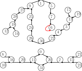
Figure 2. (A) The state transition map for the Boolean network corresponding to p53 dynamics in response to an external stress. (B) The state transition map corresponding to p53 dynamics in the absence of the external stress.

In the p53 network as shown in Figure 1, there are five nodes in total and each node only admits two values, $1$ or $0,$ representing the active and inactive state respectively. So the state set $\mathcal{S}$ is the binary expansion from 0 to 31 and in total, there are 32 states. In the state transition maps $A$ and $B$, we use decimal numbers 0-31 to indicate the gene expression. Note that we do not plot the map $C$ which is just $A^{T_{r}}.$

For each $\omega\in\Omega,$ define ${\mathcal{A}}:{\mathcal{S}}\to{\mathcal{S}}$ as follows

$${\mathcal{A}}(n,\omega)={\mathcal{A}}(1,\theta^{n-1}\omega)\circ\cdots\circ{\mathcal{A}}(1,\omega),\qquad n\in{\mathbb{N}},$$

where

$${\mathcal{A}}(1,\omega)=\begin{cases}C,&{\text{if the $0-$th position of $\omega$ is $C$};}\\ B,&{\text{if the $0-$th position of $\omega$ is $B$}.}\end{cases}$$

It is easy to see that ${\mathcal{A}}$ satisfies the cocycle property and hence it is an i.i.d dtds-RDS over $(\Omega,{\mathcal{F}},\mu,\theta)$.

Figure 2(A) shows that the map $A$ admits two attractors which are in fact two limit cycles:

(5.1) $$1\rightarrow 5\rightarrow 7\rightarrow 6\rightarrow 22\rightarrow 30\rightarrow 26\rightarrow 24\rightarrow 25\rightarrow 9\rightarrow 1,$$

(5.2) $$0\rightarrow 20\rightarrow 31\rightarrow 11\rightarrow 0,$$

respectively. Note that the map $C$ has the same attractors as the map $A.$ However, under the map $B,$ the limit cycle (5.1) collapses into a fixed point $\{6\},$ which indicates the homeostasis of the cell, whereas the limit cycle (5.2) remains the same.

The dtds-RDS ${\mathcal{A}}$ does not synchronize, because two nodes from two different basins of attractions, like 7 and 0, will never synchronize. However, according to Theorem A(ii), ${\mathcal{A}}$ is always partially synchronized, i.e., for any $\omega\in\Omega,$ there exists a partition $\eta(\omega)$ of $\mathcal{S}$ such that a pair of states belonging to the same component of $\eta$ is $\omega$-synchronized, and moreover, the cardinality of $\eta(\omega)$ equals the multiplicity $m_{1}(\omega)$ of the Lyapunov exponent $\lambda_{1}(\omega)=0.$

Using Theorem A(ii), we have the following result.

Proposition 5.1.

For $\mu$-a.e. $\omega\in\Omega$, $m_{1}(\omega)=5$, i.e., $\eta(\omega)$ consists of $5$ $\omega$-synchronized subsets.

Proof.

Let

$$\Omega_{*}=\{\omega\in\Omega:\text{the $0$-th position of $\theta^{n}\omega$ is $B$ for $n=0,\cdots,14$}\}.$$

By the definition of $\mu,$ we have

$$\mu(\Omega_{*})=(1-p)^{15}>0.$$

It is easy to see that for any $\omega\in\Omega,$ there are at least five components of $\eta(\omega),$ and four of them constitutes the attracting basin of the limits cycle (5.2), which are $W_{1}=\{31,29,21,23\},W_{2}=\{0,2,8,10\},W_{3}=\{11,15\}$ and $W_{4}=\{20,16\},$ respectively. If $\omega\in\Omega_{*}$, then the map $B$ is applied repeatedly for 14 times to all the 20 states in the basin $W_{5}$ of the limit cycle (5.1), driving all these states into the state $6$. Consequently, any two points in $W_{5}$ is $\omega$-synchronized. It follows from Theorem A(ii) that

$$m_{1}(\omega)=5,\qquad\omega\in\Omega_{*}.$$

Since $\mu(\Omega_{*})>0$ and $\mu$ is ergodic, it follows from Theorem 2.1 that $m_{1}(\omega)=5$ for $\mu$-a.e. $\omega\in\Omega.$

∎

We note that, for some other $\omega$, if, as $n$ increases, switchings between maps $A$ and $B$ at the $0$-th position of $\theta^{n}\omega$ is rather frequent, then it may happen that certain two different states in the limit cycle (5.1) never collapse, i.e., $W_{5}$ can be further decomposed into different synchronized subsets and $m_{1}(\omega)>5.$ But Proposition 5.1 says that such $\omega$’s are of zero $\mu$-measure.

Proposition 5.1 allows one to define, up to a $\mu$-null set of $\omega$’s, the equivalence relation of these gene expressions that $s_{i}\sim s_{j}$, if and only if they are in the same component of $\eta(\omega).$ To our knowledge, such concepts are new to the community of Boolean networks. The extrinsic noise-induced synchronization behaviour described above is in principle different from synchronization in mechanical systems (e.g. coupled-oscillators), because no direct interactions between cells in our model is required. It would be interesting to conduct a biological experiment to verify the partial synchronization phenomenon of multiple cells with different gene expressions exposed by the same radiation source.

In many realistic models of gene regulations, random perturbations are incorporated by making the network never “get stuck” in any state set. Generally speaking, a random gene perturbation means that any given gene has a small probability of being randomly flipped to a different state, e.g., a gene admitting value 0 can be flipped to value 1, although this only happens with very small probability [27]. Under random gene perturbations, a partially synchronized random network usually becomes a synchronized one since states from different attracting basins may collapse together due to the random flipping effect. In fact, this can be understood from Theorem A that the number of synchronized subsets is equal to the multiplicity of $0$ Lyapunov exponent, which, if being bigger than 1, is easily reduced to 1 under certain generic perturbations.

5.2. More general i.i.d networks

In the example of p53 random network, the number of state set is only 32. However, a general i.i.d random network in reality can have tens of thousands state variables. In general, to determine the multiplicity of $0$ Lyapunov exponent and the synchronized partition for a complex random network with a huge number of state variables along certain infinite sequence of maps are very difficult tasks. Nevertheless, we show below that the cardinality of the synchronized partitions, i.e. the multiplicity of $\lambda_{1}=0$ by Theorem A(ii), for a general i.i.d dtds-RDS can be estimated, at least numerically, by using the Markov chain it induces. We recall from [31] that an i.i.d dtds-RDS uniquely induces a Markov chain on ${\mathcal{S}}$ with transition probability $P=(p_{ij})_{1\leq i,j\leq k},$ where $p_{ij}=Q\{f\in\Gamma:fs_{i}=s_{j}\}$ and ${\mathcal{S}}=\{s_{1},\cdots,s_{k}\}.$

An upper bound of the multiplicity of $\lambda_{1}$ can be estimated by the number of recurrent states of the induced Markov chain as follows. Given a transit state, say $s_{i},$ of the Markov chain, almost all sample trajectories of the Markov chain visit $s_{i}$ only finite times. Then by our construction of the synchronized subsets of $\{\eta(\omega)\}$ in section 3.2, along almost every sequence of maps determined by the element $\omega$ in $\Omega,$ the component of $\eta(\omega)$ corresponding to the pre-image of $s_{i},$ ${\mathcal{A}}^{-1}(n,\omega)s_{i},$ is an empty set for $n$ sufficiently large. Consequently, the number of non-trivial components of each $\eta(\omega)$ is no more than the number of recurrent states of the induced Markov chain.

As to the lower bound, we will show that the multiplicity of $\lambda_{1}=0$ is no less than the number of recurrent classes of the induced Markov chain. In fact, algorithms has been developed to figure out the latter ones, e.g., if we treat this induced Markov chain as the digraph $G=(V,E)$, then an efficient algorithm of depth-first search of the digraph could be used to identify the recurrent communicating classes in $\mathcal{O}(|V|+|E|)$ time [15]. Recall that a recurrent class of a Markov chain is the set of all recurrent states that can go to each other with positive possibilities. In other words, any two initial states belonging to different recurrent classes will not collapse together along almost every sample trajectories of the Markov chain, i.e, they belong to different synchronized subsets. Then Theorem A(ii) implies that the multiplicity of $\lambda_{1}$ is no less than the number of recurrent classes of the induced Markov chain. Inside each recurrent class, however, it is a more delicate issue to determine whether two different states belong to a same synchronized subset, for which, the two-point motion techniques (e.g. [31]) can be used. More precisely, by applying the same sequence of maps determined by an element $\omega$ in $\Omega,$ we construct two infinite trajectories on ${\mathcal{S}}$ starting from two different initial states. For the i.i.d dtds-RDS, this two-point motion induces a Markov chain on $\mathcal{S}\times\mathcal{S}$ with transition probability $W$ being

$$W_{(s_{i},s_{j})\rightarrow(s_{m},s_{\ell})}=Q\{f\in\Gamma:fs_{i}=s_{m},fs_{j}=s_{\ell}\},\ \forall i,j,m,\ell\in\{1,\cdots,k\}.$$

Note that when $s_{i}=s_{j},s_{m}=s_{\ell}$, the transition probability is the same as that of the Markov chain induced by the i.i.d dtds-RDS, and when $s_{i}=s_{j},s_{m}\neq s_{\ell}$, the transition probability is 0. Therefore, $\{(s_{1},s_{1}),(s_{2},s_{2}),\dots,(s_{k},s_{k})\}$ is a recurrent class the Markov chain induced by $W.$ Furthermore, one can show that the i.i.d dtds-RDS synchronizes if and only if $\{(s_{1},s_{1}),(s_{2},s_{2}),\dots,(s_{k},s_{k})\}$ is the only recurrent class of the Markov chain induced by the two-point motion. If there exists any other recurrent class, then for almost every $\omega$ in $\Omega,$ the first state of any pair inside the class cannot be in the same component of the synchronized partition $\eta(\omega)$ as the second state. By Theorem A(ii), the multiplicity of $\lambda_{1}=0$ within such a recurrent class for almost every $\omega$ is at least 2. Indeed, we may better estimates the lower bound from this restriction. For instance, if $(s_{i},s_{j})$, $(s_{j},s_{\ell})$ and $(s_{i},s_{\ell})$ are in the same recurrent class other than the trivial one $\{(s_{1},s_{1}),(s_{2},s_{2}),\dots,(s_{k},s_{k})\},$ then for almost every $\omega,$ $s_{i},s_{j}$ and $s_{\ell}$ should be in three different components of $\eta(\omega),$ i.e., the multiplicity of $\lambda_{1}(\omega)=0$ in this case is at least 3. In this way, we give a lower bound for the multiplicity of the $0$ Lyapunov exponent.

We illustrate the estimation by the following example. This example of 4 states comes from [31]. The deterministic maps to choose in the i.i.d dtds-RDS are

$$\Gamma=\left\{\underbrace{\left(\begin{array}[]{c}1\rightarrow 2\\ 2\rightarrow 1\\ 3\rightarrow 4\\ 4\rightarrow 3\end{array}\right)}_{\alpha_{1}},\ \underbrace{\left(\begin{array}[]{cc}1\rightarrow 1\\ 2\rightarrow 2\\ 3\rightarrow 3\\ 4\rightarrow 4\end{array}\right)}_{\alpha_{2}},\ \underbrace{\left(\begin{array}[]{cc}1\rightarrow 4\\ 2\rightarrow 3\\ 3\rightarrow 2\\ 4\rightarrow 1\end{array}\right)}_{\alpha_{3}},\ \underbrace{\left(\begin{array}[]{cc}1\rightarrow 3\\ 2\rightarrow 4\\ 3\rightarrow 1\\ 4\rightarrow 2\end{array}\right)}_{\alpha_{4}},\ \underbrace{\left(\begin{array}[]{cc}1\rightarrow 1\\ 2\rightarrow 2\\ 3\rightarrow 3\\ 4\rightarrow 3\end{array}\right)}_{\alpha_{5}}\right\}.$$

Note that the maps $\alpha_{1},\alpha_{2},\alpha_{3},\alpha_{4}$ are permutations, while $\alpha_{5}$ is not. One can assign non-zero probability mass on each map such that the induced Markov chain is always aperiodic and irreducible. If we consider the two-point motion, then there exists a recurrent communicating class, $\{(1,3),(3,1),(2,4),(4,2),(2,3),(3,2),(4,1),(1,4)\},$ other than the trivial one. That is, if we start from any pair of these states, for some $\omega$, these two infinite long sequences will never synchronize under this i.i.d dtds-RDS. From our previous arguments, the first state cannot be in the same component as the second one in the partition $\eta(\omega),$ e.g., 1 cannot be in the same component as 3. With this restriction, a possible minimal partition could be $\eta(\omega)=\left\{\{1,2\},\{3,4\}\right\},$ which indicates that the multiplicity of $\lambda_{1}=0$ for some $\omega$ is at least 2. So we give an estimation of the lower bound of the multiplicity.

References

- [1] D. H. Ackley, G. E. Hinton, and T. J. Sejnowski, A learning algorithm for Boltzmann machine, Cog. Sci., 9, 147–169, 1985.
- [2] L. Arnold, Random Dynamical Systems, Springer, New York, 1998.
- [3] P. H. Baxendale, Statistical equilibrium and two-point motion for a stochastic flow of diffeomorphisms, Spatial Stochastic Processes: Festschrift for T. E. Harris (Ed. K. S. Alexander and J. C. Watkins), Birkhäser, Boston, 189–218, 1991.
- [4] A. Blumenthal, A volume-based approach to the multiplicative ergodic theorem on Banach spaces, Discrete Contin. Dyn. Syst. 36(5), 2377–2403, 2016.
- [5] B. Drossel, Random Boolean Networks, Reviews of Nonlinear Dynamics and Complexity (Ed. H. G, Schuster), 69–110, 2008.
- [6] F. Franco, B. Gess, and M. Scheutzow, Synchronization by noise, Prob. Th. & Related Fields, 168, 511–556, 2017.
- [7] G. Froyland, C. González-Tokman, and A. Quas, Hilbert space Lyapunov exponent stability, Trans. Amer. Math. Soc., 2019, to appear.
- [8] H. Ge, H. Qian, and M. Qian, Synchronized dynamics and nonequilibrium steady states in a stochastic yeast cell-cycle network, Math. Biosci., 211, 132–152, 2008.
- [9] H. Ge and M. Qian, Boolean network approach to negative feedback loops of the p53 pathways: synchronized dynamics and stochastic limit cycles, J. Comp. Biol., 16(1), 119–132, 2009.
- [10] C. González-Tokman, A. Quas, A concise proof of the multiplicative ergodic theorem on Banach spaces, J. Mod. Dyn. 9, 237–255, 2015.
- [11] Y. Guo, Z. You and H. Ge, Robustness and relative stability of multiple attractors in a stochastic Boolean network (in Chinese), Sci. Sin. Math., 47, 1831–1852, 2017.
- [12] J. J. Hopfield, Neural networks and physical systems with emergent collective computational abilities, Proc. Natl. Acad. Sci., 79, 2554–2558, 1982.
- [13] S. L. Harris and A. J. Levine, The p53 pathway: positive and negative feedback loops, Oncogene, 24, 2899–2908, 2005
- [14] Y. L. Jan, Équilibre statistique pour les produits de difféomorphismes aléatoires indépendants, Ann. Inst. Henri Poincare, Sect. B, 23, 111–120, 1987.
- [15] J. Jarvis and D. Shier, Graph-theoretic analysis of finite Markov chains, in: D. Shier, K. Wallenius (Eds.), Applied Mathematical Modeling: A Multidisciplinary Approach, Chapman & Hall/CRC, 2000.
- [16] S. A. Kauffman, Metabolic stability and epigenesis in randomly constructed genetic nets, J. Theor. Biol., 22(3), 437–467, 1969.
- [17] S. A. Kauffman, Homeostasis and differentiation in random genetic control networks, Nature, 224, 177–178, 1969.
- [18] Y. Kifer, Ergodic Theory of Random Transformations., Birkhäuser, Basel, 1986.
- [19] Z. Lian and K. Lu, Lyapunov exponents and invariant manifolds for random dynamical systems in a Banach space, Mem. Amer. Math. Soc. 206, 967, 2010.
- [20] K. K. Lin, Stimulus-response reliability of biological networks, Nonautonomous and Random Dynamical Systems in Life Sciences, Lecture Notes in Math. Biosci. (Ed. P. Kloeden and C. Pötzsche), 135–161, Springer, New York, 2012.
- [21] F. Li, T. Long, Y. Lu, Q. Ouyang, and C. Tang, The yeast cell-cycle network is robustly designed, Proc. Natl. Acad. Sci., 101, 4781–4786, 2004.
- [22] P. Liu and M. Qian, Smooth Ergodic Theory of Random Dynamical Systems, Springer, 2006.
- [23] Y. Ma, H. Qian, and F. X.-F. Ye, Stochastic dynamics: Models for intrinsic and extrinsic noises and their applications (in Chinese), Sci. Sin. Math., 47, 1693–1702, 2017.
- [24] J. Newman, Necessary and sufficient conditions for stable synchronization inrandom dynamical systems, Ergod. Theory Dyn. Syst., 38(5), 1857–1875, 2018.
- [25] V. I. Oseledec, A multiplicative ergodic theorem, Trans. Mosc. Math. Soc., 19(2), 179–210, 1968.
- [26] J. E. Purvis, K. W. Karhohs, C. Mock, E. Batchelor, A. Loewer and G. Lahav, p53 dynamics control cell fate, Science, 336(6087): 1440–1444, 2012.
- [27] I. Shmulevich and E. R. Dougherty, Probabilistic Boolean Networks: A Model for Gene Regulatory Networks, SIAM Press, Philadelphia, PA, 2009.
- [28] J. von Neumann, The general and logical theory of automata, Cerebral mechanisms in behavior, 1(41), 1–2, 1951.
- [29] P. Walters, An Introduction to Ergodic Theory., Springer Verlag, 1982.
- [30] S. Wolfram, A New Kind of Science, Wolfram Media, IL, 2002.
- [31] F. X.-F. Ye, Y. Wang, and H. Qian, Stochastic dynamics: Markov chains and random transformations, Discrete Cont. Dyn. Sys. B, 21, 2337–2361, 2016.
- [32] Y. Zhang, M.-P. Qian, Q. Ouyang, M. Deng, F. Li, and C. Tang, Stochastic model of yeast cell-cycle network, Physica D, 219, 35–39, 2006.