Frequency-Selective Beamforming Cancellation Design for Millimeter-Wave Full-Duplex

Abstract

The wide bandwidths offered at millimeter-wave (mmWave) frequencies have made them an attractive choice for future wireless communication systems. Recent works have presented beamforming strategies for enabling in-band full-duplex (FD) capability at mmWave even under the constraints of hybrid beamforming, extending the exciting possibilities of next-generation wireless. Existing mmWave FD designs, however, do not consider frequency-selective mmWave channels. Wideband communication at mmWave suggests that frequency-selectivity will likely be of concern since communication channels will be on the order of hundreds of megahertz or more. This has motivated the work of this paper, in which we present a frequency-selective beamforming design to enable practical wideband mmWave FD applications. In our designs, we account for the challenges associated with hybrid analog/digital beamforming such as phase shifter resolution, a desirably low number of radio frequency (RF) chains, and the frequency-flat nature of analog beamformers. We use simulation to validate our work, which indicates that spectral efficiency gains can be achieved with our design by enabling simultaneous transmission and reception in-band.

I Introduction

Future wireless networks have turned to millimeter-wave (mmWave) frequencies due to their wide bandwidths, which can offer higher rates and support more users [1]. While there are challenges associated with communication at such high frequencies, researchers have presented creative solutions that enable practical mmWave communication. Chief among these is hybrid beamforming, where the combination of a digital beamformer and an analog beamformer is used to achieve performance comparable to an unconstrained fully-digital beamformer with a reduced number of radio frequency (RF) chains [2]. The analog beamformer’s phase shifter resolution and lack of amplitude control are constraints that often complicate the hybrid approximation process [2].

The expected impacts of mmWave communication could be extended even further by equipping mmWave systems with in-band full-duplex (FD) capability—the ability for a device to simultaneously transmit and receive in-band. Such a capability offers exciting benefits over traditional half-duplex (HD) operation, where the incurred self-interference (SI) is prohibitive. Most immediately, FD operation has the potential of doubling the achievable spectral efficiency since orthogonal duplexing of transmission and reception is no longer necessary. Furthermore, at a network level, FD capability could offer significant throughput gains thanks to the transformative ability to sense the channel while transmitting, suggesting that overhead and challenges associated with conventional medium access techniques can be avoided. Additionally, the relaying associated with fifth generation (5G) network densification is a particularly suitable application for mmWave FD where a relay node could simultaneously forward and receive data.

In recent years, FD has become a reality thanks to the development of various self-interference cancellation (SIC) techniques that take advantage of the fact that a transceiver knows its own transmission, allowing it to reconstruct the SI and subtract it at the receiver. If done properly, SIC leaves a desired receive signal virtually free from SI. Almost all existing FD techniques, however, have been for systems operating at sub-$6$ GHz frequencies and cannot be applied directly to mmWave systems largely due to the numerous antennas in use and high nonlinearity. For this reason, the few existing FD designs for mmWave propose methods for mitigating SI by a means referred to as beamforming cancellation (BFC) where the transmit and receive beamformers at a transceiver are designed to avoid introducing SI [3].

Given that wide bandwidths will be used by mmWave systems, frequency-selective channels will likely be of concern. Existing BFC designs for mmWave FD, however, do not consider this frequency-selectivity, presenting designs for frequency-flat channels [3, 4]. While schemes such as orthogonal frequency-division multiplexing (OFDM) can transform a frequency-selective channel into a bank of frequency-flat subchannels, the existing BFC designs cannot be applied on a subcarrier basis due to the frequency-flat nature of the analog beamformer. For this reason, we present a frequency-selective BFC design to enable wideband mmWave FD applications. Our design captures the hybrid beamforming structure used at mmWave and incorporates its limitations during the design. We account for phase shifter resolution and a lack of amplitude control commonly associated with RF beamformers. Most importantly, our design is a frequency-selective one, enabling practical wideband FD operation at mmWave.

We use the following notation. We use bold uppercase, $\mathbf{A}$, to represent matrices. We use bold lowercase, $\mathbf{a}$, to represent column vectors. We use $(\cdot)$^∗ and $\left\lVert{\cdot}\right\rVert_{\textsf{F}}$ to represent the conjugate transpose and Frobenius norm, respectively. We use $\left[\mathbf{A}\right]_{i,j}$ to denote the element in the $i$th row and $j$th column of $\mathbf{A}$. We use $\left[\mathbf{A}\right]_{i,:}$ and $\left[\mathbf{A}\right]_{:,j}$ to denote the $i$th row and $j$th column of $\mathbf{A}$. We use $\mathcal{N}_{\mathbb{C}}\left({\mathbf{m}},{\mathbf{R}}\right)$ as a multivariate circularly symmetric complex Normal distribution having mean $\mathbf{m}$ and covariance matrix $\mathbf{R}$. We use the term “beamformer” most often to refer to a single column (rather than matrix) of beamforming weights.

II System Model

In our design, we consider a mmWave network of three nodes: $i$, $j$, and $k$. Node $i$ is a FD transceiver transmitting to $j$ while receiving from $k$ (in-band). Node $i$ is capable of simultaneously realizing independent transmit and receive beamformers at separate arrays. Nodes $j$ and $k$ are HD devices. We remark that, together, $j$ and $k$ could represent another FD device. We assume that all precoding and combining is done via fully-connected hybrid beamforming [2], where the combination of baseband and RF beamforming is used at each transmitter and receiver.

Let $N_{\textrm{t}}^{{}^{\left(m\right)}}$ $(N_{\textrm{r}}^{{}^{\left(m\right)}})$ be the number of transmit (receive) antennas at node $m\in\{i,j,k\}$. Let $L_{\textrm{t}}^{{}^{\left(m\right)}}$ $(L_{\textrm{r}}^{{}^{\left(m\right)}})$ be the number of RF chains at the transmitter (receiver) of node $m\in\{i,j,k\}$. Let all channels be frequency-selective over the band of interest. Being frequency-selective, assume the channel impulse response has length $D$ taps, and $d\in\{0,\dots,D-1\}$ represents the channel tap index (in time).

For the desired channels $\left\{\mathbf{H}_{ij}[d]\right\}$ and $\left\{\mathbf{H}_{ki}[d]\right\}$, we use the model in (1), where the multiple-input multiple-output (MIMO) channel matrix between a node’s transmit array and a different node’s receive array at tap $d$ as

$$\mathbf{H}[d]=\alpha\sum_{m=1}^{N_{\textsf{clust}}}\sum_{n=1}^{N_{\textsf{rays}}}\beta_{mn}p\left(dT_{\textrm{s}}-\tau_{mn}\right)\mathbf{a}_{\textrm{r}}(\theta_{mn})\mathbf{a}_{\textrm{t}}^{{*}}(\phi_{mn}),$$ (1)

where $\alpha=\sqrt{{N_{\textrm{t}}N_{\textrm{r}}}/{(N_{\textsf{rays}}N_{\textsf{clust}})}}$, $\mathbf{a}_{\textrm{r}}(\theta_{mn})$ and $\mathbf{a}_{\textrm{t}}(\phi_{mn})$ are the receive and transmit array responses, respectively, for ray $n$ within cluster $m$, which has some angle of arrival (AoA), $\theta_{mn}$, and angle of departure (AoD), $\phi_{mn}$ [2, 5]. The total number of clusters is $N_{\textsf{clust}}$ and the number of rays per cluster is $N_{\textsf{rays}}$. Each ray has a random gain $\beta_{mn}\sim\mathcal{N}_{\mathbb{C}}\left({0},{1}\right)$. The function $p(t)$ captures the gain at time $t$ due to pulse shaping, and $\tau_{mn}$ is the associated relative delay of ray $n$ within cluster $m$. The sampling rate of the channel is $1/T_{\textrm{s}}$ samples per second.

For the SI channel at $i$, $\{\mathbf{H}_{ii}[d]\}$, we use the Rician summation shown in (2), where $\kappa$ is the Rician factor. The line-of-sight (LOS) component $\mathbf{H}^{\textrm{LOS}}_{ii}$ is based on the spherical-wave MIMO model in [3, 6] and is frequency-flat, reserving it due to space constraints. The non-line-of-sight (NLOS) component $\mathbf{H}^{\textrm{NLOS}}_{ii}[d]$ is based on the model in (1), meaning it is frequency-selective.

$$\mathbf{H}_{ii}[d] =\sqrt{\frac{\kappa}{\kappa+1}}\mathbf{H}^{\textrm{LOS}}_{ii}+\sqrt{\frac{1}{\kappa+1}}\mathbf{H}^{\textrm{NLOS}}_{ii}[d]$$ (2)

It is worthwhile to remark that the SI channel is not well-characterized for mmWave FD systems, meaning our model may not align well with practice. The channel in (2) is full-rank, though we do not rely on its particular channel structure in our design. We expect our design will translate well to other, more practically-sound frequency-selective SI channels.

We assume OFDM is used for sufficiently transforming a frequency-selective wideband channel into a bank of $U$ frequency-flat subchannels by use of cyclic prefix of length $N_{\textrm{CP}}$. Let $u\in\{0,\dots,U-1\}$ denote the subcarrier index. Let $\bm{\mathsf{H}}_{mn}[u]$ be the frequency-flat MIMO channel matrix from node $m$ to node $n$ on subcarrier $u$ where $m,n\in\{i,j,k\}$. Having an effectively circularly-convolved channel in time, we take a $U$-point discrete Fourier transform (DFT) of the channel matrices across time to get MIMO channels across subcarriers, which are frequency-flat.

$$\bm{\mathsf{H}}[u]=\sum_{d=0}^{D-1}\mathbf{H}[d]\ e^{-\textrm{j}\frac{2\pi ud}{U}}$$ (3)

Let $\bm{\mathsf{s}}^{{}^{\left(m\right)}}[u]\sim\mathcal{N}_{\mathbb{C}}\left({\mathbf{0}},{\bm{\mathsf{R}}_{\mathsf{s}}}\right)$ be the $N_{\textrm{s}}^{{}^{\left(m\right)}}\times 1$ symbol vector transmitted on subcarrier $u$ intended for node $m\in\{i,j,k\}$, where we have assumed each subcarrier is transmitted with the same number of streams. Let $\bm{\mathsf{n}}^{{}^{\left(m\right)}}[u]\sim\mathcal{N}_{\mathbb{C}}\left({\mathbf{0}},{\sigma^{2}\bm{\mathsf{R}}_{\mathsf{n}}}\right)$ be a noise vector received by the receive array at node $m$ on subcarrier $u$, where we have assumed a common (and frequency-flat) noise covariance matrix. Defining $\sigma^{2}$ as the noise variance and letting $\bm{\mathsf{R}}_{\mathsf{n}}=\mathbf{I}$ and $\bm{\mathsf{R}}_{\mathsf{s}}=\frac{1}{U}\mathbf{I}$ provides a convenient formulation. For $m,n\in\{i,j,k\}$, we define the per subcarrier link signal-to-noise ratio (SNR) from node $m$ to node $n$ as $\mathrm{SNR}_{mn}\triangleq{P_{\textrm{tx}}^{{}^{\left(m\right)}}G^{2}_{mn}}/({\sigma^{2}B})$, where $P_{\textrm{tx}}^{{}^{\left(m\right)}}$ is the transmit power at $m$, $G^{2}_{mn}$ is the large-scale power gain of the propagation from $m$ to $n$, and $B$ is the total bandwidth. Our simulated results in Section IV are not concerned with a particular $B$; we simply use the SNR as a varied scalar quantity for evaluating our design.

Let $\bm{\mathsf{F}}_{\mathsf{BB}}^{{}^{\left(m\right)}}[u]$ $(\bm{\mathsf{W}}_{\mathsf{BB}}^{{}^{\left(m\right)}}[u])$ be the baseband precoding (combining) matrix at node $m\in\{i,j,k\}$ for subcarrier $u$. Unlike the baseband beamformers, the RF beamformers are not frequency-selective but rather frequency-flat and are not indexed per subcarrier. This fact will impact our design in Section III. Let $\bm{\mathsf{F}}_{\mathsf{RF}}^{{}^{\left(m\right)}}$ $(\bm{\mathsf{W}}_{\mathsf{RF}}^{{}^{\left(m\right)}})$ be the RF precoding (combining) matrix at $m\in\{i,j,k\}$. We impose a constant amplitude constraint on the entries of the RF beamformers representing the fact that they have phase control and no amplitude control. Further, we assume the phase shifters have finite resolution, though our design does not rely on a particular resolution.

For the sake of analysis, we impose a uniform power allocation across subcarriers and streams. To do this, we normalize the baseband precoder for each stream on subcarrier $u$ such that ${\Big{\|}\bm{\mathsf{F}}_{\mathsf{RF}}^{{}^{\left(m\right)}}\left[{\bm{\mathsf{F}}_{\mathsf{BB}}^{{}^{\left(m\right)}}[u]}\right]_{:,\ell}\Big{\|}_{\textsf{F}}}^{2}=1\ \forall\ \ell\in[0,N_{\textrm{s}}^{{}^{\left(m\right)}}-1]$ , which ensures that for all $m\in\{i,j,k\}$

$$\sum_{u=0}^{U-1}\left\lVert{\bm{\mathsf{F}}_{\mathsf{RF}}^{{}^{\left(m\right)}}{\bm{\mathsf{F}}_{\mathsf{BB}}^{{}^{\left(m\right)}}[u]}}\right\rVert_{\textsf{F}}^{2}=UN_{\textrm{s}}^{{}^{\left(m\right)}}.$$ (4)

$$\hat{\bm{\mathsf{s}}}^{{}^{\left(i\right)}}[u]= \bm{\mathsf{W}}_{\mathsf{BB}}^{{*}^{\left(i\right)}}[u]\bm{\mathsf{W}}_{\mathsf{RF}}^{{*}^{\left(i\right)}}\left(\sqrt{\mathrm{SNR}_{ki}}\ \bm{\mathsf{H}}_{ki}[u]\bm{\mathsf{F}}_{\mathsf{RF}}^{{}^{\left(k\right)}}\bm{\mathsf{F}}_{\mathsf{BB}}^{{}^{\left(k\right)}}[u]\bm{\mathsf{s}}^{{}^{\left(i\right)}}[u]+\sqrt{\mathrm{SNR}_{ii}}\ \bm{\mathsf{H}}_{ii}[u]\bm{\mathsf{F}}_{\mathsf{RF}}^{{}^{\left(i\right)}}\bm{\mathsf{F}}_{\mathsf{BB}}^{{}^{\left(i\right)}}[u]\bm{\mathsf{s}}^{{}^{\left(j\right)}}[u]+\bm{\mathsf{n}}^{{}^{\left(i\right)}}[u]\right)$$ (5)

$$\hat{\bm{\mathsf{s}}}^{{}^{\left(j\right)}}[u]= \bm{\mathsf{W}}_{\mathsf{BB}}^{{*}^{\left(j\right)}}[u]\bm{\mathsf{W}}_{\mathsf{RF}}^{{*}^{\left(j\right)}}\left(\sqrt{\mathrm{SNR}_{ij}}\ \bm{\mathsf{H}}_{ij}[u]\bm{\mathsf{F}}_{\mathsf{RF}}^{{}^{\left(i\right)}}\bm{\mathsf{F}}_{\mathsf{BB}}^{{}^{\left(i\right)}}[u]\bm{\mathsf{s}}^{{}^{\left(j\right)}}[u]+\bm{\mathsf{n}}^{{}^{\left(j\right)}}[u]\right)$$ (6)

Recall that we are considering the network where $i$ is transmitting to $j$ while $i$ is receiving from $k$ (in a FD fashion). A MIMO formulation per subcarrier gives us an estimated received symbol as (5). Notice that the transmitted signal from $i$ intended for $j$ traverses through the SI channel $\bm{\mathsf{H}}_{ii}[u]$ and is received by the combiner at $i$ being used for reception from $k$. The estimated receive symbol at $j$ from $i$ is (6), where $j$ does not encounter any SI since it is a HD device. We ignore adjacent user interference between $j$ and $k$—justified by the high path loss and directionality at mmWave.

III Frequency-Selective Beamforming Cancellation Design

$$\hat{\bm{\mathsf{F}}}_{\mathsf{BB}}^{{}^{\left(i\right)}}[u]=\left[{\left(\bm{\mathsf{H}}_{\mathrm{des}}[u]\bm{\mathsf{H}}^{{*}}_{\mathrm{des}}[u]+\frac{\mathrm{SNR}_{ii}}{\mathrm{SNR}_{ij}}\bm{\mathsf{H}}_{\mathrm{int}}[u]\bm{\mathsf{H}}^{{*}}_{\mathrm{int}}[u]+\frac{L_{\textrm{t}}^{{}^{\left(i\right)}}}{\mathrm{SNR}_{ij}}\mathbf{I}\right)^{-1}\bm{\mathsf{H}}^{{*}}_{\mathrm{des}}[u]}\right]_{:,0:N_{\textrm{s}}^{{}^{\left(i\right)}}-1}$$ (23)

In this section, we present a frequency-selective BFC design for the system described in Section II. Our goal is to design precoding and combining strategies across nodes $i$, $j$, and $k$ that enable FD operation at $i$ by mitigating the SI it would otherwise incur. In this design, we assume perfect channel state information (CSI) across nodes. There are two primary factors to keep in mind throughout our design. First, the hybrid beamforming architecture involves a baseband and an RF beamformer at each transmitter and each receiver. Second, being a frequency-selective one, our design will be on a per subcarrier basis: the baseband beamformer is frequency-selective but the RF beamformer is frequency-flat and would ideally be designed to satisfy all subcarriers to some degree.

III-A Frequency-Selective Hybrid Approximation

We first present a frequency-selective hybrid approximation algorithm that we will use throughout our design. This algorithm extends orthogonal matching pursuit (OMP) based hybrid approximation [7] from the conventional frequency-flat setting to a frequency-selective one. In OMP based hybrid approximation, the constraints of the RF beamformer (e.g., phase quantization and constant amplitude) are captured in a codebook matrix $\bm{\mathsf{A}}_{\mathsf{RF}}$ whose columns are beamformers satisfying the constraints. Conventional OMP hybrid approximation is represented in (7), where a fully-digital, frequency-flat beamforming matrix $\bm{\mathsf{X}}$ is being approximated by the product $\bm{\mathsf{X}}_{\mathsf{RF}}\bm{\mathsf{X}}_{\mathsf{BB}}$ for a given codebook $\bm{\mathsf{A}}_{\mathsf{RF}}$ and number of RF chains $N_{\textrm{RF}}$. We leave the precise definition of OMP hybrid approximation to [7]. In short, OMP hybrid approximation builds $\bm{\mathsf{X}}_{\mathsf{RF}}$ column-by-column by choosing the columns in $\bm{\mathsf{A}}_{\mathsf{RF}}$ that correlate the best with the columns of $\bm{\mathsf{X}}$, appropriately updating its search based on the chosen RF beamformers as the algorithm progresses. Note that, when transmitting/receiving $N_{\textrm{s}}$ streams on $N_{\textrm{a}}$ antennas, we have $\bm{\mathsf{X}}\in\mathbb{C}^{N_{\textrm{a}}\times N_{\textrm{s}}}$, then $\bm{\mathsf{X}}_{\mathsf{RF}}\in\mathbb{C}^{N_{\textrm{a}}\times N_{\textrm{RF}}}$ and $\bm{\mathsf{X}}_{\mathsf{BB}}\in\mathbb{C}^{N_{\textrm{RF}}\times N_{\textrm{s}}}$.

$$\left(\bm{\mathsf{X}}_{\mathsf{RF}},\bm{\mathsf{X}}_{\mathsf{BB}}\right)=\text{omp\_hybrid\_approx}\left(\bm{\mathsf{X}},\bm{\mathsf{A}}_{\mathsf{RF}},N_{\textrm{RF}}\right)$$ (7)

To extend this conventional frequency-flat OMP hybrid approximation to a frequency-selective one, we present the following. Given a set of fully-digital beamforming matrices $\left\{\bm{\mathsf{X}}[u]\right\}_{u=0}^{U-1}$, indexed by subcarrier, we construct the matrix $\bar{\bm{\mathsf{X}}}$ by horizontally stacking the matrices as follows.

$$\bar{\bm{\mathsf{X}}}=\begin{bmatrix}{\bm{\mathsf{X}}[0]}&{\bm{\mathsf{X}}[1]}&\cdots&{\bm{\mathsf{X}}[U-1]}\end{bmatrix}\in\mathbb{C}^{N_{\textrm{a}}\times UN_{\textrm{s}}}$$ (8)

We then invoke conventional OMP hybrid approximation using (7) on $\bar{\bm{\mathsf{X}}}$ instead of $\bm{\mathsf{X}}$, as shown in (9). The effect of this is that the OMP hybrid approximation algorithm extracts the beamformers in $\bm{\mathsf{A}}_{\mathsf{RF}}$ that satisfy beamformers across all subcarriers.

$$\left(\bm{\mathsf{X}}_{\mathsf{RF}},\bar{\bm{\mathsf{X}}}_{\mathsf{BB}}\right)=\text{omp\_hybrid}\left(\bar{\bm{\mathsf{X}}},\bm{\mathsf{A}}_{\mathsf{RF}},N_{\textrm{RF}}\right)$$ (9)

The returned baseband matrix $\bar{\bm{\mathsf{X}}}_{\mathsf{BB}}\in\mathbb{C}^{N_{\textrm{RF}}\times UN_{\textrm{s}}}$ is then of the fashion

$$\bar{\bm{\mathsf{X}}}_{\mathsf{BB}} =\begin{bmatrix}{\bm{\mathsf{X}}_{\mathsf{BB}}[0]}&{\bm{\mathsf{X}}_{\mathsf{BB}}[1]}&\cdots&{\bm{\mathsf{X}}_{\mathsf{BB}}[U-1]}\end{bmatrix},$$ (10)

where the baseband beamforming matrices per subcarrier are horizontally stacked. The returned RF matrix $\bm{\mathsf{X}}_{\mathsf{RF}}$ is of the standard fashion having dimensions number of antennas by number of RF chains. We refer to this method as frequency-selective OMP hybrid approximation (FS-OMP) throughout our design.

III-B Precoding and Combining at the Half-Duplex Nodes

Taking the singular value decomposition (SVD) of the desired channels on subcarrier $u$, we get

$$\bm{\mathsf{H}}_{ki}[u] =\bm{\mathsf{U}}_{\bm{\mathsf{H}}_{ki}}[u]\ \bm{\mathsf{\Sigma}}_{\bm{\mathsf{H}}_{ki}}[u]\ \bm{\mathsf{V}}^{{*}}_{\bm{\mathsf{H}}_{ki}}[u]$$ (11)

$$\bm{\mathsf{H}}_{ij}[u] =\bm{\mathsf{U}}_{\bm{\mathsf{H}}_{ij}}[u]\ \bm{\mathsf{\Sigma}}_{\bm{\mathsf{H}}_{ij}}[u]\ \bm{\mathsf{V}}^{{*}}_{\bm{\mathsf{H}}_{ij}}[u],$$ (12)

where the singular values in both are decreasing along their diagonals. We set the desired precoder at $k$ and the desired combiner at $j$ to the so-called eigenbeamformers

$$\bm{\mathsf{F}}^{{}^{\left(k\right)}}[u] =\left[{\bm{\mathsf{V}}_{\bm{\mathsf{H}}_{ki}}[u]}\right]_{:,0:N_{\textrm{s}}^{{}^{\left(k\right)}}-1}$$ (13)

$$\bm{\mathsf{W}}^{{}^{\left(j\right)}}[u] =\left[{\bm{\mathsf{U}}_{\bm{\mathsf{H}}_{ij}}[u]}\right]_{:,0:N_{\textrm{s}}^{{}^{\left(i\right)}}-1},$$ (14)

where $N_{\textrm{s}}^{{}^{\left(k\right)}},N_{\textrm{s}}^{{}^{\left(i\right)}}$ streams are being communicated on each subcarrier’s strongest so-called eigenchannels. Being fully-digital beamforming matrices, we now seek to represent them in a hybrid fashion. To do this, we employ FS-OMP by building $\bar{\bm{\mathsf{F}}}^{{}^{\left(k\right)}}$ from $\{\bm{\mathsf{F}}^{{}^{\left(k\right)}}[u]\}$ and $\bar{\bm{\mathsf{W}}}^{{}^{\left(j\right)}}$ from $\{\bm{\mathsf{W}}^{{}^{\left(j\right)}}[u]\}$, as described by (8). Invoking (9) on each gives us

$$\left(\bm{\mathsf{F}}_{\mathsf{RF}}^{{}^{\left(k\right)}},\bar{\bm{\mathsf{F}}}_{\mathsf{BB}}^{{}^{\left(k\right)}}\right)=\text{omp\_hybrid}\left(\bar{\bm{\mathsf{F}}}^{{}^{\left(k\right)}},\bm{\mathsf{A}}_{\mathsf{RF}}^{{}^{\left(k\right)}},L_{\textrm{t}}^{{}^{\left(k\right)}}\right)$$ (15)

$$\left(\bm{\mathsf{W}}_{\mathsf{RF}}^{{}^{\left(j\right)}},\bar{\bm{\mathsf{W}}}_{\mathsf{BB}}^{{}^{\left(j\right)}}\right)=\text{omp\_hybrid}\left(\bar{\bm{\mathsf{W}}}^{{}^{\left(j\right)}},\bm{\mathsf{A}}_{\mathsf{RF}}^{{}^{\left(j\right)}},L_{\textrm{r}}^{{}^{\left(j\right)}}\right),$$ (16)

where $\bm{\mathsf{A}}_{\mathsf{RF}}^{{}^{\left(m\right)}}$ is the beamforming codebook matrix at $m\in\{j,k\}$. Unpacking $\bar{\bm{\mathsf{F}}}_{\mathsf{BB}}^{{}^{\left(k\right)}}$ and $\bar{\bm{\mathsf{W}}}_{\mathsf{BB}}^{{}^{\left(j\right)}}$ gives us the baseband beamforming matrix at $k$ and $j$, respectively, for each subcarrier as described by (10). We fix these hybrid beamformers at the half-duplex nodes $k$ and $j$, concluding their design.

III-C Precoding and Combining at the Full-Duplex Node

Having set the precoder at $k$ and the combiner at $j$, we focus our attention to designing the precoder and combiner at $i$. We begin with considering the eigenbeamformers associated with receiving from $k$ and transmitting to $j$. Referring to (11) and (12),

$$\bm{\mathsf{W}}^{{}^{\left(i\right)}}[u] =\left[{\bm{\mathsf{U}}_{\bm{\mathsf{H}}_{ki}}[u]}\right]_{:,0:N_{\textrm{s}}^{{}^{\left(k\right)}}-1}$$ (17)

$$\bm{\mathsf{F}}^{{}^{\left(i\right)}}[u] =\left[{\bm{\mathsf{V}}_{\bm{\mathsf{H}}_{ij}}[u]}\right]_{:,0:N_{\textrm{s}}^{{}^{\left(i\right)}}-1}.$$ (18)

We invoke FS-OMP to get the hybrid approximations of each and unpack the baseband beamformers per subcarrier to get

$$\left(\bm{\mathsf{W}}_{\mathsf{RF}}^{{}^{\left(i\right)}},\left\{\bm{\mathsf{W}}_{\mathsf{BB}}^{{}^{\left(i\right)}}[u]\right\}\right)$$ (19)

$$\left(\bm{\mathsf{F}}_{\mathsf{RF}}^{{}^{\left(i\right)}},\left\{\bm{\mathsf{F}}_{\mathsf{BB}}^{{}^{\left(i\right)}}[u]\right\}\right).$$ (20)

Now, we choose to fix the baseband and RF combiners to those in (19) and the RF precoder to that in (20). The final stage of our design is in tailoring the baseband precoder on each subcarrier to avoid introducing SI.

We desire our choice of precoder $\{\hat{\bm{\mathsf{F}}}_{\mathsf{BB}}^{{}^{\left(i\right)}}[u]\}$ to be such that the received SI is mitigated on a per subcarrier basis. We have chosen to fix $\bm{\mathsf{F}}_{\mathsf{RF}}^{{}^{\left(i\right)}}$ due to its constant amplitude constraint and quantized phase shifters. Thus, we have set every baseband and RF beamformer at each transmitter and receiver except the baseband precoder at $i$. This motivates us to define the effective SI channel

$$\bm{\mathsf{H}}_{\mathrm{int}}[u]\triangleq\bm{\mathsf{W}}_{\mathsf{BB}}^{{*}^{\left(i\right)}}[u]\bm{\mathsf{W}}_{\mathsf{RF}}^{{*}^{\left(i\right)}}\bm{\mathsf{H}}_{ii}[u]\bm{\mathsf{F}}_{\mathsf{RF}}^{{}^{\left(i\right)}}$$ (21)

and the effective desired channel from $i$ to $j$ as

$$\bm{\mathsf{H}}_{\mathrm{des}}[u]\triangleq\bm{\mathsf{W}}_{\mathsf{BB}}^{{*}^{\left(j\right)}}[u]\bm{\mathsf{W}}_{\mathsf{RF}}^{{*}^{\left(j\right)}}\bm{\mathsf{H}}_{ij}[u]\bm{\mathsf{F}}_{\mathsf{RF}}^{{}^{\left(i\right)}}$$ (22)

With these definitions, we recognize that a desirable design of the baseband precoder at $i$ resembles that of a regularized zero-forcing (RZF) transmitter (or commonly called a linear minimum mean square error (LMMSE) transmitter) [8]. In such a precoder design, the signal-to-leakage-plus-noise ratio is the metric of choice, rather than the signal-to-interference-plus-noise ratio which would apply to the combiner design. A RZF design resembles an LMMSE one, where trading off matched filtering for interference suppression is done dynamically based on the SNRs involved. We invoke (23), where ${\hat{\bm{\mathsf{F}}}_{\mathsf{BB}}}^{{}^{\left(i\right)}}[u]$ is our baseband precoder at $i$ on subcarrier $u$ with BFC applied.

Upon normalizing all our beamformers according to our power constraint, this concludes our design, having set the RF beamformers at all nodes and the baseband beamformers on all subcarriers at all nodes.

III-D Design Remarks

We note that an RZF, like an LMMSE, will be driven to a zero-forcing (ZF) solution when the interference dominates. Such a scenario is common in FD applications since the SI channel is often much stronger than the desired channels. This indicates that ZF designs like that in [3] will likely be similar to the solution arrived at by a RZF design. For this reason, we expect that appropriate dimensionality should be offered to the baseband precoder to allow a ZF solution requiring $L_{\textrm{t}}^{{}^{\left(i\right)}}\geq(N_{\textrm{s}}^{{}^{\left(i\right)}}+N_{\textrm{s}}^{{}^{\left(k\right)}})$ to successfully design a precoder at $i$ that avoids the interference in (21) completely. This is because there are $N_{\textrm{s}}^{{}^{\left(k\right)}}$ dimensions being received by the combiner and another $N_{\textrm{s}}^{{}^{\left(i\right)}}$ dimensions are needed in the null space to transmit on.

IV Simulation and Results

To validate our design, we simulated three scenarios using the following parameters, where each scenario is a variant of the three node network referenced throughout. The number of clusters and rays per cluster is the same for each tap. Ray delays for a given tap are uniformly distributed between sampling instances $(dT_{\textrm{s}})$, where $f_{\textrm{s}}=1/T_{\textrm{s}}=2$ GSPS. For the desired channels, the number of clusters and rays per cluster are uniformly distributed on $[1,6]$ and $[1,10]$, respectively. Each ray’s AoD and AoA are Laplacian distributed with a standard deviation of $0.2$ and a mean according to its cluster mean AoD and AoA, which is uniformly distributed on $[0,\pi]$. We consider a root raised cosine pulse shape where $\beta=1$. The maximum delay of frequency-selective channels $D$ is varied throughout our simulated scenarios, though we consistently use an OFDM cyclic prefix of length $N_{\textrm{CP}}=D/4$.

We transmit two streams on each link, i.e., $N_{\textrm{s}}^{{}^{\left(k\right)}}=N_{\textrm{s}}^{{}^{\left(i\right)}}=2$. Horizontal half-wavelength uniform linear arrays (ULAs) are used at all nodes, where the number of transmit antennas and the number of receive antennas are both $32$. The transmit and receive arrays at $i$ are vertically stacked with a separation of $10$ wavelengths, a factor only of concern to create the spherical-wave MIMO SI channel in (2). For the SI channel, we use a Rician factor of $\kappa=10$ dB and a NLOS channel with the same parameters as the simulated desired channels, except with fewer clusters and rays. The number of clusters is uniformly distributed on $[1,3]$, and the number of rays per cluster is uniformly distributed on $[1,6]$. In all simulated scenarios, we let $\mathrm{SNR}_{ii}=80$ dB due to close proximity of the transmit and receive arrays at $i$.

During OMP hybrid approximation, we use a DFT codebook matrix across at all nodes. Note that this choice implicitly suggests that the phase shifters have a resolution of at least $2\pi/N_{\textrm{a}}$, where $N_{\textrm{a}}$ is the number of antennas at the beamformer being approximated.

TABLE I: Simulated Scenarios and their Parameters

Scenario	$U$	$L_{\textrm{t}}^{{}^{\left(i\right)}}$	$L_{\textrm{r}}^{{}^{\left(i\right)}}$	$L_{\textrm{r}}^{{}^{\left(j\right)}}$	$L_{\textrm{t}}^{{}^{\left(k\right)}}$
Equal users, low selectivity	$8$	$6$	$2$	$2$	$2$
Equal users, high selectivity	$128$	$8$	$4$	$4$	$4$
Disparate users, low selectivity	$8$	$6$	$2$	$2$	$2$

Important Benchmarks

Our primary metric for evaluating our design is the sum of the spectral efficiencies from $i$ to $j$ and from $k$ to $i$.

IV-1 Ideal Full-Duplex

To evaluate our design, we compare its performance to that of an ideal FD system, where the two links simultaneously operate interference-free. There are two ideal FD scenarios to consider: (i) two non-interfering links operating with fully-digital eigenbeamformers and (ii) two non-interfering links operating with hybrid-approximated eigenbeamformers. We consider both because there will be some loss attributed to frequency-selective hybrid approximation and to BFC design—plotting them against our achieved results will indicate our design’s relative performance.

IV-2 Half-Duplex

For evaluating the HD spectral efficiency, we again consider both a fully-digital and a hybrid case, both using eigenbeamformers. In both, it is important to note that we assume equal time-sharing of the medium by the two links. (Of course, equal time-sharing may not satisfy a particular application’s sense of fairness.) Given equal time-sharing, the fully-digital HD sum spectral efficiency is half of the fully-digital ideal FD one. The hybrid HD sum spectral efficiency is half of the hybrid ideal FD one. It is the goal of our FD design to outperform HD operation.

Scenario #1: Similar Users in a Mildly Selective Channel

In this simulated scenario, we have considered equal SNRs on the links from $k$ to $i$ and from $i$ to $j$, i.e., $\mathrm{SNR}_{ki}=\mathrm{SNR}_{ij}$. Such a scenario could correspond to a case where $k$ and $j$ are collocated, perhaps together comprising a single FD node. (However, we remark that we have not considered reciprocal channels.) Additionally, we have considered a mildly selective channel where $D=8$ and $U=8$. As indicated by the first row of Table I, we have allotted $6$ RF chains to our precoder at $i$. This provides the dimensionality for sufficient performance of our design, as described in our design remarks, where we will use the additional RF chains for mitigating SI.

The results of this scenario are shown in Figure 1, which shows the sum spectral efficiency of the two links as a function of their SNRs. The two variants of ideal FD operation are shown, where the fully-digital case outperforms the hybrid one, as expected, due to imperfect hybrid approximation by OMP. Also included are the fully-digital and hybrid HD cases. Between HD and ideal FD operation lies our achieved FD sum spectral efficiency. The goal of FD operation, of course, is to outperform HD operation, which is achieved by our design. In fact, the gain that can be seen over HD operation by our design is almost completely attributed to the spectral efficiency of the link from $i$ to $j$ since the link from $k$ to $i$ is relatively unaffected by our design. This is thanks to the ZF nature of the precoder at $i$ given that $\mathrm{SNR}_{ii}$ is so strong.

We now comment on our frequency-selective hybrid approximation algorithm based on OMP (i.e., FS-OMP). In this case we have considered a mildly selective channel, meaning that there are fewer subcarriers. For this reason, it is expected that frequency-selective hybrid approximation is more likely to offer better performance since the frequency-flat RF beamformer has to satisfy fewer subcarriers. In general, increasing the number of RF chains will improve the accuracy of hybrid approximation, which is supported in the next simulated scenario. Hybrid approximation (which is inevitably imperfect) will always be outperformed by a fully-digital solution free of constraints. This can be observed in Figure 1 between the two ideal FD cases and between the two HD cases. At best, our design can aim for the performance seen by the hybrid-approximated ideal FD spectral efficiency. Given all of this, we remark that our frequency-selective BFC design could be enhanced with improvements to hybrid approximation.

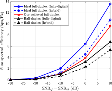
Figure 1: Results of simulating Scenario #1 showing sum spectral efficiency as a function of $\mathrm{SNR}_{ij}=\mathrm{SNR}_{ki}$ when $\mathrm{SNR}_{ii}=80$ dB.

Scenario #2: Similar Users in a Highly Selective Channel

In this scenario, we again consider users with equal SNRs, i.e., $\mathrm{SNR}_{ij}=\mathrm{SNR}_{ki}$. However, this time, we consider a highly selective channel where the number of channel taps is $D=128$ and the number of subcarriers is accordingly $U=128$. Most immediately, we remark that high frequency-selectivity will introduce challenges in hybrid approximation: the frequency-flat RF beamformers must satisfy many subcarriers. To account for this, we increase the number of RF chains at each transmitter and each receiver compared to the mildly selective case in Scenario #1. The parameters used are shown in the second row of Table I.

The results of this scenario are in Figure 2. Comparing this to the results of Scenario #1, we make a few points. First, we remark that such high selectivity introduces significant challenges in hybrid approximation, even with the increased number of RF chains. This introduces sizable gaps between a fully-digital curve and its respective hybrid curve. For this reason, it’s important that we compare our design to the FD and HD hybrid cases rather than to the fully-digital ones. Our design does quite well in approaching the hybrid ideal FD spectral efficiency, nearly doubling the hybrid HD spectral efficiency. These results indicate that our design extends from a mildly selective scenario to a highly selective one quite well.

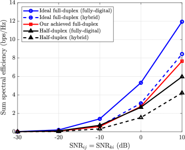
Figure 2: Results of simulating Scenario #2 showing sum spectral efficiency as a function of $\mathrm{SNR}_{ij}=\mathrm{SNR}_{ki}$ when $\mathrm{SNR}_{ii}=80$ dB.

Scenario #3: Disparate Users in a Mildly Selective Channel

In this scenario, we consider the case when the link from $k$ to $i$ is $30$ dB weaker than the link from $i$ to $j$, i.e., $\mathrm{SNR}_{ij}=\mathrm{SNR}_{ki}+30$ dB. Recall that our design sacrifices some performance on the link from $i$ to $j$ while aiming to preserve the link from $k$ to $i$. We consider user disparity to see how this loss on $i$ to $j$ affects the overall performance of our design. The simulation parameters for this can be seen in Table I, where we have allotted $6$ RF chains to the transmitter to exaggerate our point. A lower number of RF chains at the transmitter yield similar, but less convincing, results. We remark that we forgo showing the alternative, when $k$ to $i$ is stronger than $i$ to $j$, because such a scenario is favored by our design by preserving the stronger link.

The results of this scenario are shown in Figure 3, where the sum spectral efficiency is shown as a function of $\mathrm{SNR}_{ij}$. The achieved sum spectral efficiency during FD operation with our design is comprised of the degraded link on $i$ to $j$ and the relatively unaffected link from $k$ to $i$. However, since $\mathrm{SNR}_{ki}$ is much weaker than $\mathrm{SNR}_{ij}$, the losses on $i$ to $j$ are magnified, given our assumption of equal time-sharing for HD operation. Even with $30$ dB of disparity, the sum spectral efficiency achieved by our FD design outperforms HD operation. These results indicate that our design, while somewhat lopsided in that it only tailors precoder in its design, manages to produce meaningful gains over HD, both fully-digital and hybrid.

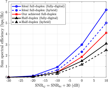
Figure 3: Results of simulating Scenario #3 showing sum spectral efficiency as a function of $\mathrm{SNR}_{ij}=\mathrm{SNR}_{ki}+30$ dB when $\mathrm{SNR}_{ii}=80$ dB.

V Conclusion

In this paper, we presented a frequency-selective beamforming strategy that enables simultaneous in-band transmission and reception at a mmWave transceiver employing fully-connected hybrid beamforming. Our design leverages existing OMP based hybrid approximation to account for quantized phase shifters and lack of amplitude control associated with RF beamforming. Our strategy addresses the frequency-selectivity that mmWave systems are likely see over wideband communication, mitigating SI on each subcarrier while maintaining service to the desired users. Results from simulation indicate that our strategy offers FD spectral efficiency gains in various channel conditions.

References

- [1] J. G. Andrews, S. Buzzi, W. Choi, S. V. Hanly, A. Lozano, A. C. K. Soong, and J. C. Zhang, “What will 5G be?” IEEE Journal on Selected Areas in Communications, vol. 32, no. 6, pp. 1065–1082, Jun 2014.
- [2] R. W. Heath, N. Gonzalez-Prelcic, S. Rangan, W. Roh, and A. M. Sayeed, “An overview of signal processing techniques for millimeter wave MIMO systems,” IEEE Journal of Selected Topics in Signal Processing, vol. 10, no. 3, pp. 436–453, Apr. 2016.
- [3] I. P. Roberts and S. Vishwanath, “Beamforming cancellation design for millimeter-wave full-duplex,” in Proceedings of the 2019 IEEE Global Communications Conference: Signal Processing for Communications, Waikoloa, HI, USA, Dec. 2019.
- [4] K. Satyanarayana, et al., “Hybrid beamforming design for full-duplex millimeter wave communication,” IEEE Transactions on Vehicular Technology, vol. 68, no. 2, pp. 1394–1404, Feb. 2019.
- [5] A. Alkhateeb and R. W. Heath, “Frequency selective hybrid precoding for limited feedback millimeter wave systems,” IEEE Transactions on Communications, vol. 64, no. 5, pp. 1801–1818, May 2016.
- [6] J. S. Jiang and M. A. Ingram, “Spherical-wave model for short-range MIMO,” IEEE Transactions on Communications, vol. 53, no. 9, pp. 1534–1541, Sep. 2005.
- [7] O. E. Ayach, S. Rajagopal, S. Abu-Surra, Z. Pi, and R. W. Heath, “Spatially sparse precoding in millimeter wave MIMO systems,” IEEE Transactions on Wireless Communications, vol. 13, no. 3, pp. 1499–1513, Mar. 2014.
- [8] R. W. Heath Jr. and A. Lozano, Foundations of MIMO Communication. Cambridge University Press, 2018.