A Gibbs sampler for a class of random convex polytopes

Abstract

We present a Gibbs sampler for the Dempster–Shafer (DS) approach to statistical inference for Categorical distributions. The DS framework extends the Bayesian approach, allows in particular the use of partial prior information, and yields three-valued uncertainty assessments representing probabilities “for”, “against”, and “don’t know” about formal assertions of interest. The proposed algorithm targets the distribution of a class of random convex polytopes which encapsulate the DS inference. The sampler relies on an equivalence between the iterative constraints of the vertex configuration and the non-negativity of cycles in a fully connected directed graph. Illustrations include the testing of independence in $2\times 2$ contingency tables and parameter estimation of the linkage model.

1 Introduction

Consider observed counts of $K$ possible categories, denoted by $N_{1},\ldots,N_{K}$ and summing to $N$. We assume that these counts are sums of independent draws from a Categorical distribution. The goal is to infer the associated parameters $\theta$ in the simplex of dimension $K$ and to forecast future observations. The setting is most familiar to statisticians and if $K$ is small relative to $N$, and without further information about $\theta$, the story is somewhat simple with the maximum likelihood estimator being both very intuitive and efficient. The plot thickens quickly if $N$ is small or indeterminate, if partial prior information is available, if observations are imperfect, or if additional constraints are imposed, especially when uncertainty quantification is simultaneously sought (Fitzpatrick and Scott, 1987; Berger and Bernardo, 1992; Sison and Glaz, 1995; Liu, 2000; Lang, 2004; Chafai and Concordet, 2009; Dunson and Xing, 2009). As any probability distribution on a finite unordered set is necessarily Categorical, the setting often arises as part of more elaborate procedures. Besides, the canonical nature of Categorical distributions has made them a common test bed for various approaches to inference (Walley, 1996; Bernard, 1998).

The Dempster–Shafer (DS) theory is a framework for probabilistic reasoning based on observed data and modeling of knowledge. In the DS framework, inferences on user-defined assertions are expressed probabilistically. These assertions can be statements concerning parameters (“the parameter belongs to a certain set”) or concerning future observations. Contrary to Bayesian inference, no prior distribution is strictly required, and partial prior specification is allowed (see Section 4.2). Rather than posterior probabilities, DS inference yields three-valued assessments of uncertainty, namely probabilities “for”, “against”, and “don’t know” associated with the assertion of interest, and denoted by $(\texttt{p},\texttt{q},\texttt{r})$ (see Section 2.2). In his pioneering work, Dempster (1963, 1966, 1967, 1968) developed the idea of upper and lower probabilities for assertions of interest. Together with the contributions of Shafer (1976, 1979), the approach became known as the Dempster–Shafer (DS) theory of belief functions. The framework has various connections to other ways of obtaining lower and upper probabilities and to robust Bayesian inference (Wasserman, 1990). Over the past decades, the DS theory saw various applications in signal processing, computer vision and machine learning (see e.g., Bloch, 1996; Vasseur et al., 1999; Denoeux, 2000; Basir and Yuan, 2007; Denoeux, 2008; Díaz-Más et al., 2010). As outlined in Dempster (2008, 2014) the DS framework is an ambitious tool for carrying out statistical inferences in scientific practice. During the developments of DS, Categorical distributions were front and center due to their generality and relevance to ubiquitous statistical objects such as contingency tables.

The computation required by the DS approach for Categorical distributions proved to be demanding. The approach involves distributions of convex polytopes within the simplex, some properties of which were found in Dempster (1966, 1968, 1972). Unfortunately, no closed-form joint distribution of the vertices has been found, hindering both theoretical developments and numerical approximations. The challenge prompted Denœux (2006) to comment that, “Dempster studied the trinomial case […] However, the application of these results to compute the marginal belief function […] has proved, so far and to our knowledge, mathematically intractable.” Likewise, Lawrence et al. (2009) commented: “[…] his method for the Multinomial model is seldom used, partly because of its computational complexity.” Over the past fifty years, the literature saw a handful of alternative methods for Categorical inference via generalized fiducial inference (Hannig et al., 2016; Liu and Hannig, 2016) the Imprecise Dirichlet Model (Walley, 1996), the Dirichlet-DSM method (Lawrence et al., 2009), the vector-valued Poisson model (Edlefsen et al., 2009), and the Poisson-projection method for Multinomial data (Gong, 2018, unpublished PhD thesis). The latter three methods were motivated in part to circumvent the computational hurdle put forward by the original DS formulation. The present article aims at filling that gap by proposing an algorithm that carries out the computation proposed in Dempster (1966, 1972). The presentation does not assume previous knowledge on DS inference.

Section 2 introduces the formal setup. Section 3 presents an equivalence between constraints arising in the definition of the problem and the existence of “negative cycles” (defined in Section 3.2) in a certain weighted graph, that leads to a Gibbs sampler. Various illustrations and extensions are laid out in Section 4. Section 5 concerns applications to $2\times 2$ contingency tables and the linkage model. Elements of future research are discussed in Section 6. Code in R (R Core Team, 2018) is available at github.com/pierrejacob/dempsterpolytope to reproduce the figures of the article.

2 Inference in Categorical distributions

We describe inference in Categorical distributions as proposed in Dempster (1966), using the following notation. The observations are $\mathbf{x}=(x_{n})_{n\in[N]}$, with $x_{n}\in[K]$ for all $n\in[N]$, where $[m]$ denotes the set $\{1,\ldots,m\}$ for $m\geq 1$. The number of categories is $K$. The $K$-dimensional simplex is $\Delta=\{z\in\mathbb{R}_{+}^{K}\colon\;\sum_{k=1}^{K}z_{k}=1\}$. The set of measurable subsets of $\Delta$ is denoted by $\mathcal{B}(\Delta)$. We denote the vertices of $\Delta$ by $V_{1},\ldots,V_{K}$. In barycentric coordinates, $V_{k}$ is a $K$-vector with $k$-th entry equal to one and other entries equal to zero. A polytope is a set of points $z\in\mathbb{R}^{K}$ satisfying linear inequalities, of the form $Mz\leq c$ understood component-wise, and where $M$ is a matrix with $K$ columns and $c$ is a vector. For a given $\mathbf{x}\in[K]^{N}$, $\mathcal{I}_{k}$ is the set of indices $\{n\in[N]\colon x_{n}=k\}$. The counts are $N_{k}=|\mathcal{I}_{k}|$ and $\sum_{k\in[K]}N_{k}=N$. Coordinates of $u_{n}\in\Delta$ are denoted by $u_{n,k}$ for $k\in[K]$. The volume of a set $A$ is denoted by $\text{Vol}(A)$. The uniform variable $Z$ over $\mathcal{S}$ is written $Z\sim\mathcal{S}$.

2.1 Sampling mechanism and feasible sets

The goal is to infer the parameters $\theta=(\theta_{1},\ldots,\theta_{K})\in\Delta$ of a Categorical distribution using observation $\mathbf{x}=(x_{n})_{n\in[N]}\in[K]^{N}$. Viewing $x_{n}$ as a random variable, the model states $\mathbb{P}(x_{n}=k)=\theta_{k}$ for all $k\in[K]$, $n\in[N]$. Generating draws from a Categorical distribution can be done in different ways. In the DS approach, the choice of sampling mechanism of the observable data has an impact on inference of the parameters, a feature that distinguishes DS from likelihood-based approaches, and aligns it with fiducial (Fisher, 1935; Hannig et al., 2016), structural (Fraser, 1968), and functional (Dawid and Stone, 1982) approaches. Appendix A illustrates this impact in a simple setting. We follow Dempster (1966) and consider the following sampling mechanism for $x_{n}$, which is invariant by permutation of the labels of the categories; it is equivalent to the “Gumbel-max trick” (Maddison et al., 2014) as explained in Appendix B. Given $\theta$, for each $k\in[K]$, define $\Delta_{k}(\theta)$ to be a “subsimplex” obtained as the polytope with the same vertices as $\Delta$ except that vertex $V_{k}$ is replaced by $\theta$. The sets $(\Delta_{k}(\theta))_{k\in[K]}$ form a partition of $\Delta$, shown in Figure 1a. It can be checked that $\text{Vol}(\Delta_{k}(\theta))=\theta_{k}$. Then, introduce $u_{n}\sim\Delta$, and define $x_{n}$ as

$$x_{n}=\sum_{k\in[K]}k\mathds{1}(u_{n}\in\Delta_{k}(\theta)).$$ (2.1)

In other words, $x_{n}$ is the unique index $k\in[K]$ such that $u_{n}$ belongs to $\Delta_{k}(\theta)$. Since $\text{Vol}(\Delta_{k}(\theta))=\theta_{k}$, $x_{n}$ indeed follows the Categorical distribution with parameter $\theta$. Lemma 2.1 recalls a useful characterization of $\Delta_{k}(\theta)$.

Lemma 2.1.

(Lemma 5.2 in Dempster (1966)). For $k\in[K]$, $\theta\in\Delta$ and $u_{n}\in\Delta$, $u_{n}\in\Delta_{k}(\theta)$ if and only if $u_{n,\ell}/u_{n,k}\geq\theta_{\ell}/\theta_{k}$ for all $\ell\in[K]$.

Given fixed observations $\mathbf{x}=(x_{n})_{n\in[N]}$, the sampling mechanism in (2.1) can be turned into constraints on the values of $\mathbf{u}=(u_{n})_{n\in[N]}$ and $\theta$ that could have led to the observations. A central piece of the machinery is the following set,

$$\mathcal{R}_{\mathbf{x}}=\left\{(u_{1},\ldots,u_{N})\in\Delta^{N}\colon\;\exists\theta\in\Delta\quad\forall n\in[N]\quad u_{n}\in\Delta_{x_{n}}(\theta)\right\}.$$ (2.2)

It is the set of all possible realizations of $\mathbf{u}$ which could have produced the data $\mathbf{x}$ for (at least) some $\theta$, via the specified sampling mechanism. Given a realization of $\mathbf{u}\in\mathcal{R}_{\mathbf{x}}$ by definition there is a non-empty “feasible” set $\mathcal{F}(\mathbf{u})\subset\Delta$ defined as

$$\mathcal{F}(\mathbf{u})=\left\{\theta\in\Delta\colon\;\forall n\in[N]\quad u_{n}\in\Delta_{x_{n}}(\theta)\right\}.$$ (2.3)

On the other hand if $\mathbf{u}$ is an arbitrary point in $\Delta^{N}$ then $\mathcal{F}(\mathbf{u})$ defined above can be empty. For example $\mathbf{u}=(u_{1},u_{2},u_{3})$ shown in Figure 1b leads to an empty $\mathcal{F}(\mathbf{u})$ for the observations $x_{1}=1,x_{2}=3,x_{3}=2$. The goal of the proposed method is to obtain non-empty sets $\mathcal{F}(\mathbf{u})$, as illustrated for another data set in Figure 2a. We can rewrite (2.2) as $\mathcal{R}_{\mathbf{x}}=\{\mathbf{u}\colon\mathcal{F}(\mathbf{u})\neq\emptyset\}$.

The ingredients introduced thus far specify the “source” of a belief function (e.g. Wasserman, 1990). The central object of interest here is the distribution of the random sets $\mathcal{F}(\mathbf{u})$ conditional on them being non-empty. We consider the uniform distribution on $\mathcal{R}_{\mathbf{x}}$ denoted by $\nu_{\mathbf{x}}$, with density

$$\forall u_{1},\ldots,u_{N}\in\Delta^{N}\quad\nu_{\mathbf{x}}(u_{1},\ldots,u_{N})=\text{Vol}\left(\mathcal{R}_{\mathbf{x}}\right)^{-1}\mathds{1}\left((u_{1},\ldots,u_{N})\in\mathcal{R}_{\mathbf{x}}\right).$$ (2.4)

Our main contribution is an algorithm to sample $\mathbf{u}$ from $\nu_{\mathbf{x}}$. The sets $\mathcal{F}(\mathbf{u})$ obtained when $\mathbf{u}\sim\nu_{\mathbf{x}}$ constitute the class of random convex polytopes studied in Dempster (1972) and referred to in the title of the present article. The distribution $\nu_{\mathbf{x}}$ is also the result of Dempster’s rule of combination (Dempster, 1967) applied to the information provided separately by each of the $N$ observations.

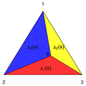
(a)

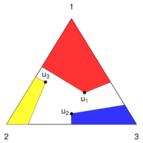
(b)

Figure 1: Partition of $\Delta$ into $(\Delta_{k}(\theta))_{k\in[K]}$ in 1a, with $K=3$. Each point $u_{n}\in\Delta$ defines, for a fixed $x_{n}\in[K]$, a set of $\theta\in\Delta$ such that $u_{n}\in\Delta_{x_{n}}(\theta)$; three such sets are colored in 1b, for $x_{1}=1,x_{2}=3,x_{3}=2$. Here, no $\theta\in\Delta$ is such that $u_{n}\in\Delta_{x_{n}}(\theta)$ for $n=1,2,3$.

2.2 Inference using random sets

We recall briefly how random sets can be processed into “lower” and “upper” probabilities as in Dempster (1966), or into “belief” and “plausibility” as in Shafer (1976, 1990); Wasserman (1990), or $(\texttt{p},\texttt{q},\texttt{r})$ probabilities as in Dempster (2008). The user provides a measurable subset $\Sigma\in\mathcal{B}(\Delta)$ corresponding to an “assertion” of interest about the parameter, for instance $\Sigma=\{\theta\in\Delta\colon\theta_{1}\leq 1/3\}$, or $\Sigma=\{\theta\in\Delta\colon\theta_{1}/\theta_{2}>\theta_{3}/\theta_{4}\}$. The belief function assigns a value to each $\Sigma\in\mathcal{B}(\Delta)$ defined as $\text{Bel}(\Sigma)=\nu_{\mathbf{x}}(\{\mathbf{u}\colon\mathcal{F}(\mathbf{u})\subset\Sigma\})$. This can be called lower probability and written $\underline{P}(\Sigma)$. The upper probability or “plausibility” $\bar{P}(\Sigma)$ is defined as $1-\underline{P}(\Sigma^{c})$, or equivalently $\nu_{\mathbf{x}}(\{\mathbf{u}\colon\mathcal{F}(\mathbf{u})\cap\Sigma\neq\emptyset)\}$. Bayesian inference is recovered exactly when combining the distribution of $\mathcal{F}(\mathbf{u})$ obtained from $\mathbf{x}$ with a prior distribution on $\theta$, see Dempster (1968) and Section 4.2. Following Dempster (2008) DS inference can be summarized via the probability triple $(\texttt{p},\texttt{q},\texttt{r})$:

$$\texttt{p}(\Sigma)=\underline{P}(\Sigma),\quad\texttt{q}(\Sigma)=1-\bar{P}(\Sigma),\quad\texttt{r}(\Sigma)=\bar{P}(\Sigma)-\underline{P}(\Sigma),$$ (2.5)

with $\texttt{p}+\texttt{q}+\texttt{r}=1$ for all $\Sigma$, quantifying support “for”, “against”, and “don’t know” about the assertion $\Sigma$. As argued in Dempster (2008); Gong (2019), the triple $(\texttt{p},\texttt{q},\texttt{r})$ draws a stochastic parallel to the three-valued logic, with r representing weight of evidence in a third, indeterminate logical state. A p or q value close to 1 is interpreted as strong evidence towards $\Sigma$ or $\Sigma^{c}$, respectively. A large r suggests that the model and data are structurally deficient in making precise judgment about the assertion $\Sigma$ or its negation.

Sampling methods enable approximations of these probabilities via standard Monte Carlo arguments. A simple strategy is to draw $(u_{n})_{n\in[N]}$ from the uniform on $\Delta^{N}$ until $\mathcal{F}(\mathbf{u})$ is non-empty. However the rejection rate would be prohibitively high as $N$ increases. Some properties of $\nu_{\mathbf{x}}$ have been obtained in Dempster (1966, 1972). For example, Equation (2.1) in Dempster (1972) states that, for a fixed $\theta\in\Delta$, $\nu_{\mathbf{x}}(\{\mathbf{u}\colon\theta\in\mathcal{F}(\mathbf{u})\})$ is equal to the Multinomial probability mass function with parameter $\theta$ evaluated at $N_{1},\ldots,N_{K}$. Equation (2.5) in Dempster (1972) gives the expected volume of $\mathcal{F}(\mathbf{u})$. Dempster (1972) also obtains the distribution of vertices of $\mathcal{F}(\mathbf{u})$ under $\mathbf{u}\sim\nu_{\mathbf{x}}$ with smallest and largest coordinate $\theta_{k}$ for any $k\in[K]$, which are Dirichlet distributions. These enable the approximation of $(\texttt{p},\texttt{q},\texttt{r})$ for certain assertions, including the sets $\{\theta\colon\theta_{k}\in[0,c]\}$ for arbitrary $c\in[0,1]$. However, for general assertions the joint distribution of all vertices of $\mathcal{F}(\mathbf{u})$ under $\mathbf{u}\sim\nu_{\mathbf{x}}$ is necessary, as in the case of both applications in Section 5.

3 Proposed Gibbs sampler

Input: $k\in[K]$, $\theta\in\Delta$, and the vertices of $\Delta$ denoted by $(V_{\ell})_{\ell\in[K]}$.

• Sample $(w_{1},\ldots,w_{K})$ uniformly on $\Delta$,
  e.g. $\tilde{w}_{\ell}\sim\text{Exponential}(1)$ for all $\ell\in[K]$ and $w_{\ell}=\tilde{w}_{\ell}/\sum_{j=1}^{K}\tilde{w}_{j}$.

• Define the point $z=w_{k}\theta+\sum_{\ell\neq k}w_{\ell}V_{\ell}$,
  e.g. $z_{k}=w_{k}\theta_{k}$ and $z_{\ell}=w_{k}\theta_{\ell}+w_{\ell}$ for $\ell\neq k$.

• Return $z$, a uniformly distributed point in $\Delta_{k}(\theta)$.

Algorithm 1 Uniform sampling in $\Delta_{k}(\theta)$.

3.1 Strategy

The proposed algorithm is a Markov chain Monte Carlo (MCMC) method targeting $\nu_{\mathbf{x}}$, thus referred to as the target distribution. At the initial step, we set $\theta^{(0)}$ arbitrarily in $\Delta$, for example a draw from a Dirichlet distribution. Given $\theta^{(0)}$ we can sample, for $k\in[K]$ and $n\in\mathcal{I}_{k}$, $u_{n}\sim\Delta_{k}(\theta^{(0)})$. Then $\mathbf{u}=(u_{n})_{n\in[N]}$ is in $\mathcal{R}_{\mathbf{x}}$ because $\theta^{(0)}$ is in $\mathcal{F}(\mathbf{u})$ by construction. Sampling uniformly over $\Delta_{k}(\theta)$ can be done following equation (5.7) in Dempster (1966), as recalled in Algorithm 1. In this section we assume that $N_{k}=|\mathcal{I}_{k}|\geq 1$ for all $k\in[K]$, and describe how to handle empty categories in Section 4.1.

We draw components of $\mathbf{u}$ from conditional distributions given the other components under $\nu_{\mathbf{x}}$, namely we draw $\mathbf{u}_{\mathcal{I}_{k}}=(u_{n})_{n\in\mathcal{I}_{k}}$ for $k\in[K]$ from $\nu_{\mathbf{x}}(d\mathbf{u}_{\mathcal{I}_{k}}|\mathbf{u}_{[N]\setminus\mathcal{I}_{k}})$. Drawing $\mathbf{u}_{\mathcal{I}_{k}}$ from this conditional distribution will constitute an iteration of a Gibbs sampler, illustrated in Figure 2 for the data $N_{1}=2,N_{2}=3,N_{3}=1$. Figure 2a shows a sample $\mathbf{u}\in\mathcal{R}_{\mathbf{x}}$, with each $u_{n}$ colored according to $x_{n}\in[K]$. Sampling from $\nu_{\mathbf{x}}(d\mathbf{u}_{\mathcal{I}_{k}}|\mathbf{u}_{[N]\setminus\mathcal{I}_{k}})$ can be understood as drawing all the points of the same color conditional on the other points. The overall Gibbs sampler cycles through the $K$ categories to generate a sequence of draws $\mathbf{u}^{(t)}$ that converges to $\nu_{\mathbf{x}}$ as $t\to\infty$, for example in distribution. To each $\mathbf{u}^{(t)}$ is associated a feasible set $\mathcal{F}(\mathbf{u}^{(t)})$ that can contribute to the approximation of $(\texttt{p},\texttt{q},\texttt{r})$ triples described in Section 2.2. The next question is how to sample from the adequate conditional distributions. Towards this aim we will draw on a representation of $\mathcal{R}_{\mathbf{x}}$ connected to the presence of “negative cycles” in a complete graph with $K$ vertices.

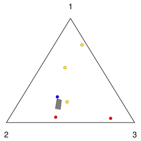
(a)

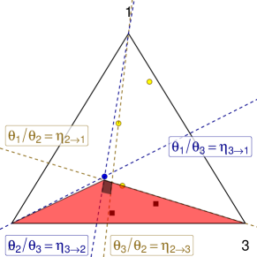
(b)

Figure 2: Given $\mathbf{u}\in\mathcal{R}_{\mathbf{x}}$ (shown in 2a), drop components $\mathbf{u}_{\mathcal{I}_{k}}$ for some $k\in[K]$ (the red dots in 2a) and draw new components $\mathbf{u}_{\mathcal{I}_{k}}$ (the red squares in 2b) from their conditional distribution identified in Proposition 3.2 with support represented by the shaded triangle.

3.2 Non-emptiness of feasible sets

We can represent $\mathcal{R}_{\mathbf{x}}$ without mention of the existence of some $\theta\in\Delta$ as in (2.2), but instead with explicit constraints on the components of $\mathbf{u}$. We first find an equivalent representation of $\theta\in\mathcal{F}(\mathbf{u})$ for a fixed $\mathbf{u}$. By definition $\theta\in\mathcal{F}(\mathbf{u})$ satisfies for all $n\in[N]\;u_{n}\in\Delta_{x_{n}}(\theta)$. For each $k\in[K]$, using Lemma 2.1 we write

$$\forall n\in\mathcal{I}_{k}\quad\forall\ell\in[K]\setminus\{k\}\quad\frac{u_{n,\ell}}{u_{n,k}}\geq\frac{\theta_{\ell}}{\theta_{k}}\quad\Leftrightarrow\quad\forall\ell\in[K]\setminus\{k\}\quad\min_{n\in\mathcal{I}_{k}}\frac{u_{n,\ell}}{u_{n,k}}\geq\frac{\theta_{\ell}}{\theta_{k}}.$$

This prompts the definition

$$\forall k\in[K]\quad\forall\ell\in[K]\quad\eta_{k\to\ell}(\mathbf{u})=\min_{n\in\mathcal{I}_{k}}\frac{u_{n,\ell}}{u_{n,k}}.$$ (3.1)

Observe that the values $(\eta_{k\to\ell}(\mathbf{u}))$ depend on the observations through the sets $(\mathcal{I}_{k})$. At this point, $\theta\in\mathcal{F}(\mathbf{u})$ is equivalent to $\theta_{\ell}/\theta_{k}\leq\eta_{k\to\ell}(\mathbf{u})$ for $\ell,k\in[K]$. Next assume $\theta\in\mathcal{F}(\mathbf{u})$ and consider some implications. First, for all $k,\ell$

$$\frac{\theta_{\ell}}{\theta_{k}}\leq\eta_{k\to\ell}(\mathbf{u}),\quad\text{and}\quad\frac{\theta_{k}}{\theta_{\ell}}\leq\eta_{\ell\to k}(\mathbf{u}),\quad\text{thus}\quad\eta_{k\to\ell}(\mathbf{u})\eta_{\ell\to k}(\mathbf{u})\geq 1.$$

If $K\geq 3$ we can write $\theta_{\ell}/\theta_{k}$ as $(\theta_{\ell}/\theta_{j})(\theta_{j}/\theta_{k})$, and apply a similar reasoning to obtain the inequalities $\eta_{\ell\to k}(\mathbf{u})\eta_{k\to j}(\mathbf{u})\eta_{j\to\ell}(\mathbf{u})\geq 1$ for all $k,\ell,j$. Overall we can write, for all $K\geq 2$, with any number $L$ of indices $j_{1},\ldots,j_{L}\in[K]$, the following constraints:

$$\forall L\in[K]\quad\forall j_{1},\ldots,j_{L}\in[K]\quad\eta_{j_{1}\to j_{2}}(\mathbf{u})\eta_{j_{2}\to j_{3}}(\mathbf{u})\ldots\eta_{j_{L}\to j_{1}}(\mathbf{u})\geq 1.$$ (3.2)

Hereafter we drop “$(\mathbf{u})$” from the notation for clarity. The case $L=1$ gives inequalities $\eta_{k\to k}\geq 1$ which are always satisfied since $\eta_{k\to k}=1$ following (3.1). Furthermore, it suffices to consider only indices $j_{1},\ldots,j_{L}$ that are unique, otherwise the associated inequality in (3.2) is implied by inequalities associated with smaller values of $L$.

At this point, we observe a fruitful connection between (3.2) and directed graphs. The indices in $[K]$ can be viewed as vertices of a fully connected directed graph. Directed edges are ordered pairs $(j_{1},j_{2})$. We associate the product $\eta_{j_{1}\to j_{2}}\eta_{j_{2}\to j_{3}}\ldots\eta_{j_{L}\to j_{1}}$ with a sequence of edges, $(j_{1},j_{2})$, $(j_{2},j_{3})$, up to $(j_{L},j_{1})$. That sequence forms a path from vertex $j_{1}$ back to vertex $j_{1}$, of length $L$, in other words a directed cycle of length $L$. Define $w_{k\to\ell}=\log\eta_{k\to\ell}$ for all $k,\ell\in[K]$, and treat it as the weight of edge $(k,\ell)$. Then the inequality (3.2) is equivalent to $w_{j_{1}\to j_{2}}+w_{j_{2}\to j_{3}}+\ldots+w_{j_{L}\to j_{1}}\geq 0$. The sum of weights along a path is called its “value”. The inequalities in (3.2) are then equivalent to all cycles in the graph having non-negative values. See Figure 3 for an illustration for $K=3$ of the equivalent conception of constraints in (3.2) as graph cycle values. Detecting whether graphs contain cycles with negative values, called “negative cycles”, can be done with the Bellman–Ford algorithm (Bang-Jensen and Gutin, 2008).

At this point we have established that $\theta\in\mathcal{F}(\mathbf{u})$ implies the inequalities of (3.2), which can be understood as constraints on the weights of a graph. Our next result states that the converse also holds.

Proposition 3.1.

There exists $\theta\in\Delta$ satisfying $\theta_{\ell}/\theta_{k}\leq\eta_{k\to\ell}$ for all $k,\ell\in[K]$ if and only if the values $(\eta_{k\to\ell})$ satisfy

$$\forall L\in[K]\quad\forall j_{1},\ldots,j_{L}\in[K]\quad\eta_{j_{1}\to j_{2}}\eta_{j_{2}\to j_{3}}\ldots\eta_{j_{L}\to j_{1}}\geq 1.$$ (3.3)

Furthermore it suffices to restrict (3.3) to distinct indices $j_{1},\ldots,j_{L}$.

Proof.

The proof of the reverse implication explicitly constructs a feasible $\theta$ based on the values $(\eta_{k\to\ell})$, assuming that they satisfy (3.3). Introduce the fully connected graph with $K$ vertices, with weight $\log\eta_{k\to\ell}$ on edge $(k,\ell)$. Thanks to $(\eta_{k\to\ell})$ satisfying (3.3), there are no negative cycles thus one cannot decrease the value of a path by appending a cycle to it. Since there are only finitely many paths without cycles there is a finite minimal value over all paths from $k$ to $\ell$, which we denote by $\min(k\to\ell)$. In other words (3.3) implies that $\min(k\to\ell)$ is finite.

We choose a vertex in $[K]$ arbitrarily, for instance vertex $K$. We define $\theta$ by $\theta_{k}=\exp(\min(K\to k))$ and then by normalizing the entries so that $\theta\in\Delta$. We can write $\min(K\to\ell)\leq\min(K\to k)+\log\eta_{k\to\ell}$, because the right hand side is the value of a path from $K$ to $\ell$ (via $k$), while the left hand side is the smallest value over all such paths. Upon taking the exponential, the above inequality is equivalent to $\theta_{\ell}/\theta_{k}\leq\eta_{k\to\ell}$. ∎

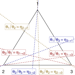
(a)

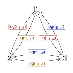
(b)

Figure 3: Two views on the constraints in (3.2). In 3a the values $\eta_{k\to\ell}$ define linear constraints $\theta_{\ell}/\theta_{k}=\eta_{k\to\ell}$. In 3b the log values are weights on the edges of a complete directed graph.

3.3 Conditional distributions

Thanks to Proposition 3.1 we can write $\mathcal{R}_{\mathbf{x}}$ defined in (2.2) as the set of $\mathbf{u}$ for which the values $\eta_{k\to\ell}$ satisfy (3.3), with $\eta_{k\to\ell}$ defined in (3.1). We next provide a representation of the conditional distribution of $\mathbf{u}_{\mathcal{I}_{k}}$ under $\nu_{\mathbf{x}}$ that is convenient for sampling purposes.

Proposition 3.2.

Let $\mathbf{u}=(u_{1},\ldots,u_{N})\in\mathcal{R}_{\mathbf{x}}$, and define $\eta_{k\to\ell}=\min_{n\in\mathcal{I}_{k}}u_{n,\ell}/u_{n,k}$ for all $k,\ell\in[K]$. Let $k\in[K]$. Define for $\ell\in[K]$,

$$\theta_{\ell}=\frac{\exp(-\min(\ell\to k))}{\sum_{\ell^{\prime}\in[K]}\exp(-\min(\ell^{\prime}\to k))}$$ (3.4)

where $\min(\ell\to k)$ is the minimum value over all paths from $\ell$ to $k$, in a fully connected directed graph with weight $\log\eta_{j\to\ell}$ on edge $(j,\ell)$. Then, $\nu_{\mathbf{x}}(d\mathbf{u}_{\mathcal{I}_{k}}|\mathbf{u}_{[N]\setminus\mathcal{I}_{k}})$ is the uniform distribution on $\Delta_{k}(\theta)^{N_{k}}$.

In other words $\nu_{\mathbf{x}}(d\mathbf{u}_{\mathcal{I}_{k}}|\mathbf{u}_{[N]\setminus\mathcal{I}_{k}})$ is the product measure with each component $u_{n}$ following the uniform distribution on $\Delta_{k}(\theta)$, with $\theta$ defined in (3.4). The proposition is key to the implementation of the proposed Gibbs sampler.

Proof.

We consider an arbitrary $k\in[K]$, and assume that $\mathbf{u}\in\mathcal{R}_{\mathbf{x}}$. Listing the inequalities in (3.3) that involve the index $k$ and separating the terms $\eta_{k\to\ell}$ from the others, we obtain

$$\forall\ell\in[K]\quad \quad\eta_{k\to\ell}\geq\eta_{\ell\to k}^{-1}\;,$$ (3.5)

$$\forall\ell\in[K]\quad\forall L\in[K-2]\quad\forall j_{1},\ldots,j_{L}\in[K]\setminus\{k,\ell\} \quad\eta_{k\to\ell}\geq\left(\eta_{\ell\to j_{1}}\ldots\eta_{j_{L}\to k}\right)^{-1}.$$ (3.6)

Thus, for $\mathbf{u}$ to remain in $\mathcal{R}_{\mathbf{x}}$ after updating its components $\mathbf{u}_{\mathcal{I}_{k}}$, it is enough to check that the ratios $u_{n,\ell}/u_{n,k}$ for $\ell\in[K]$ and $n\in\mathcal{I}_{k}$ are lower bounded as above.

The finiteness of $\min(\ell\to k)$ results from the same reasoning as in the proof of Proposition 3.1. Note that $\min(\ell\to k)$ can be constructed without the entries $\mathbf{u}_{\mathcal{I}_{k}}$ of $\mathbf{u}$, because the shortest path from $\ell$ to $k$ should pay no attention to any directed edges that stem from $k$, and the entries $\mathbf{u}_{\mathcal{I}_{k}}$ inform only the weights of edges stemming from $k$. Thus we can define $\theta$ as in (3.4).

We next show that the support of $\nu_{\mathbf{x}}(d\mathbf{u}_{\mathcal{I}_{k}}|\mathbf{u}_{[N]\setminus\mathcal{I}_{k}})$ is exactly $\Delta_{k}(\theta)^{N_{k}}$. Let $\mathbf{u}_{\mathcal{I}_{k}}\in\Delta_{k}(\theta)^{N_{k}}$. By Lemma 2.1 and the definition of $\theta$, we have

$$\forall\ell\in[K]\quad\min_{n\in\mathcal{I}_{k}}\frac{u_{n,\ell}}{u_{n,k}}\geq\exp(-\min(\ell\to k)).$$

But $\exp(-\min(\ell\to k))=(\exp(\min(\ell\to k)))^{-1}$ is greater than $(\eta_{\ell\to j_{1}}\ldots\eta_{j_{L}\to k})^{-1}$ for any path $\ell\to j_{1}\ldots j_{L}\to k$. Thus, with $\eta_{k\to\ell}=\min_{n\in\mathcal{I}_{k}}u_{n,\ell}/u_{n,k}$, inequalities (3.5)-(3.6) are satisfied. Proposition 3.1 guarantees that $\mathbf{u}$ is in $\mathcal{R}_{\mathbf{x}}$, thus $\Delta_{k}(\theta)^{N_{k}}$ is contained in the support of $\nu_{\mathbf{x}}(d\mathbf{u}_{\mathcal{I}_{k}}|\mathbf{u}_{[N]\setminus\mathcal{I}_{k}})$.

Let us show the reverse inclusion by considering $\mathbf{u}_{\mathcal{I}_{k}}\notin\Delta_{k}(\theta)^{N_{k}}$. There, for some $n\in\mathcal{I}_{k}$ and some $\ell\in[K]$, we have $u_{n,\ell}/u_{n,k}<\exp(-\min(\ell\to k))$. Denote by $\ell\to j_{1}\ldots j_{L}\to k$ the path attaining the value $\min(\ell\to k)$. We obtain $\eta_{k\to\ell}\leq u_{n,\ell}/u_{n,k}<(\eta_{\ell\to j_{1}}\ldots\eta_{j_{L}\to k})^{-1}$, and thus $\eta_{k\to\ell}\eta_{\ell\to j_{1}}\ldots\eta_{j_{L}\to k}<1$, in other words some inequalities in (3.3) are not satisfied and thus, by Proposition 3.1, $\mathbf{u}$ is not in $\mathcal{R}_{\mathbf{x}}$. ∎

Proposition 3.2 provides a strategy to sample from the conditional distributions of interest, provided that we can obtain $\theta\in\Delta$ in (3.4), which involves $\min(\ell\to k)$ for all $\ell$. These can be obtained from shortest path algorithms such as Bellman–Ford implemented in igraph (Csardi and Nepusz, 2006). Alternatively we can view $\theta$ in (3.4) as the solution of the linear program,

$$\text{max}\left\{\theta_{k}\colon\theta\in\Delta\quad\forall j\neq k\quad\forall i\neq j\quad\frac{\theta_{i}}{\theta_{j}}\leq\eta_{j\to i}\right\}.$$ (3.7)

This has a simple interpretation: $\theta$ in (3.4) is precisely the vertex of $\mathcal{F}(\mathbf{u})$ with the largest $k$-th component. The equivalence between shortest path problems and linear programs is well known. Implementations are provided in lpsolve (Berkelaar et al., 2004; Konis, 2014).

The Gibbs sampler is described in Algorithm 2. Its outputs include $\mathbf{u}^{(t)}$ converging to $\nu_{\mathbf{x}}$ in distribution as $t\to\infty$, as well as the associated values of $(\eta_{k\to\ell}^{(t)})$ from which we can obtain the sets $\mathcal{F}(\mathbf{u}^{(t)})$ as $\{\theta\in\Delta:\theta_{\ell}/\theta_{k}\leq\eta_{k\to\ell}^{(t)}\;\forall k,\ell\in[K]\}$. Such sets can be stored in “half-space representation” or as a list of vertices in $\Delta$, obtained by vertex enumeration (Avis and Fukuda, 1992). Convenient functions to store and manipulate polytopes can be found in rcdd (Geyer and Meeden, 2008; Fukuda, 1997). We run $100$ iterations of the sampler and record elapsed seconds for different values of $N$ and $K$. Medians over $50$ experiments are reported in Figure 4, for counts set to $\lfloor N/K\rfloor$ in each category.

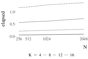
(a)

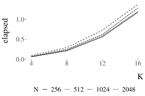
(b)

Figure 4: Elapsed time in seconds for 100 iterations of the sampler. In 4a, elapsed time as a function of $N$, for different $K$. In 4b, elapsed time as a function of $K$, for different $N$.

1. Set $\theta^{(0)}$ in $\Delta$, and for all $k\in[K]$, all $n\in\mathcal{I}_{k}$, sample $u_{n}^{(0)}\sim\Delta_{k}(\theta^{(0)})$ (Algorithm 1).

2. Compute $\eta_{k\to\ell}^{(0)}=\min_{n\in\mathcal{I}_{k}}u_{n,\ell}^{(0)}/u_{n,k}^{(0)}$ for all $k,\ell\in[K]$.

3. At iteration $t\geq 1$,

   1. Set $\eta_{k\to\ell}^{(t)}\leftarrow\eta_{k\to\ell}^{(t-1)}$ for all $k,\ell\in[K]$.

   2. For category $k\in[K]$,

      1. Compute $\theta\in\Delta$ from the values $(\eta_{j\to\ell}^{(t)})$ according to (3.4),

      2. either by computing shortest paths or by solving a linear program (3.7).

      3. For each $n\in\mathcal{I}_{k}$, sample $u^{(t)}_{n}\sim\Delta_{k}(\theta)$ (Algorithm 1).

      4. Set $\eta_{k\to\ell}^{(t)}\leftarrow\min_{n\in\mathcal{I}_{k}}u^{(t)}_{n,\ell}/u^{(t)}_{n,k}$, for all $\ell\neq k$.

Algorithm 2 Gibbs sampler for Categorical inference in the Dempster–Shafer framework.
Input: observations $\mathbf{x}\in[K]^{N}$, defining index sets $\mathcal{I}_{k}=\{n\in[N]:x_{n}=k\}$ for $k\in[K]$.
Output: sequence $(\mathbf{u}^{(t)})_{t\geq 0}$ converging to $\nu_{\mathbf{x}}$, the uniform distribution on $\mathcal{R}_{\mathbf{x}}$.

3.4 Convergence to stationarity

A common question to all MCMC algorithms is the rate of convergence to stationary (Jerrum, 1998; Roberts and Rosenthal, 2004), which here might depend on $K$ and the observed counts $N_{1},\ldots,N_{K}$. In the simplest case where $K=2$, with counts $N_{1}\geq 1,N_{2}\geq 1$, we obtain an upper bound on the mixing time of the chain in the 1-Wasserstein metric (e.g. Gibbs, 2004) as detailed in Appendix C. We find that the upper bound increases at most linearly with the total count $N=N_{1}+N_{2}$. The extension of this theoretical result to arbitrary $K\geq 3$ is left as an open question.

For arbitrary $K$ we use the empirical approach of Biswas et al. (2019), that provides estimated upper bounds on the total variation distance (TV) between $\mathbf{u}^{(t)}$ at iteration $t$ and $\nu_{\mathbf{x}}$. These upper bounds are obtained as empirical averages over independent runs of coupled Markov chains; see Appendix D for a brief description of the approach. For $K=4,8,12,16$, we construct synthetic data sets with $10$ observations in each category and estimate upper bounds for a range of $t$ shown in Figure 5a. The number of iterations required for convergence seems to be stable in $K$. Next, we set $K=5$ and consider $10,20,30,40$ counts in each category, leading to $N$ varying between $50$ and $200$. Figure 5b shows the associated upper bounds, that increase with $N$.

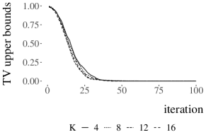
(a)

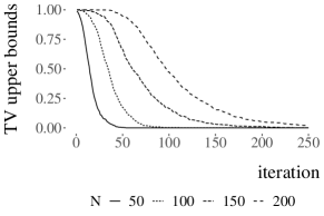
(b)

Figure 5: Upper bounds on the TV distance between $\mathbf{u}^{(t)}$ and $\nu_{\mathbf{x}}$ against $t$. Figure 5a shows varying $K$ with $10$ counts in each category. Figure 5b shows varying $N$ with $K=5$ and $N/K$ counts in each category.

4 Adding categories, observations and priors

4.1 Adding empty categories

We describe how to add empty and remove empty categories based on the output of the Gibbs sampler. Suppose that we have draws $\mathbf{u}$ distributed according to the target $\nu_{\mathbf{x}}$ associated with a data set $\mathbf{x}\in[K]^{N}$ with $K$ non-empty categories. We add a category $K+1$ with $\mathcal{I}_{K+1}=\emptyset$, $N_{K+1}=0$, and consider how to obtain samples $\mathbf{u}^{\prime}$ from the corresponding target $\nu_{\mathbf{x}^{\prime}}$. Recall that a variable $(u_{1},\ldots,u_{K})$ following Dirichlet$(1,\ldots,1)$ is equal in distribution to the vector with $\ell$-th entry $w_{\ell}/\sum_{j\in[K]}w_{j}$ for $\ell\in[K]$, where $(w_{\ell})_{\ell\in[K]}$ are independent Exponential(1). Given $(u_{1},\ldots,u_{K})\sim\Delta$ consider the following procedure. First, draw $s\sim\text{Gamma}(K,1)$, define $w_{\ell}=s\times u_{\ell}$ for $\ell\in[K]$, and draw $w_{K+1}\sim\text{Exponential}(1)$. Then define $u^{\prime}_{\ell}=w_{\ell}/\sum_{j\in[K+1]}w_{j}$ for $\ell\in[K+1]$. The resulting vector $\mathbf{u}^{\prime}=(u^{\prime}_{1},\ldots,u^{\prime}_{K+1})$ is uniformly distributed on the probability simplex with $K+1$ vertices denoted by $\Delta^{\prime}$. Since $u^{\prime}_{\ell}/u^{\prime}_{k}=u_{\ell}/u_{k}$ for all $k,\ell\in[K]$, if $(u_{1},\ldots,u_{K})$ satisfies certain constraints on ratios $u_{\ell}/u_{k}$, the same constraints are satisfied for $(u^{\prime}_{1},\ldots,u^{\prime}_{K+1})$. Thus $\mathbf{u}^{\prime}\sim\nu_{\mathbf{x}^{\prime}}$.

We can also remove empty categories. Assume that category $K+1$ is empty and that we have draws $\mathbf{u}^{\prime}\sim\nu_{\mathbf{x}^{\prime}}$. For each $u^{\prime}_{n}$, drop the $(K+1)$-th component $u^{\prime}_{n,K+1}$, and define $u_{n}$ by normalizing the remaining $K$ components. The resulting $\mathbf{u}$ follows $\nu_{\mathbf{x}}$. Importantly, inferences obtained from $\nu_{\mathbf{x}}$ are not necessarily identical to those obtained from $\nu_{\mathbf{x}^{\prime}}$. This is illustrated with Figure 6, showing the $(\texttt{p},\texttt{q},\texttt{r})$ probabilities associated with the sets $\{\theta\colon\theta_{1}\in[0,c)\}$ and $\{\theta\colon\log\theta_{1}/\theta_{2}\in(-\infty,c)\}$, for the counts $(4,3)$ and $(4,3,0)$.

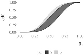
(a)

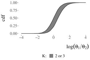
(b)

Figure 6: Inference on $\theta_{1}$ (6a) and on $\log(\theta_{1}/\theta_{2})$ (6b) using counts $(4,3)$ ($K=2$) and $(4,3,0)$ ($K=3$). Including an empty third category modifies the inference on $\theta_{1}$ but not on $\theta_{1}/\theta_{2}$.

4.2 Adding partial prior information

In the DS framework multiple sources of information can be merged using Dempster’s rule of combination (Dempster (Section 5, 1967); Wasserman (Section 2, 1990)). If two sources yield random sets $\mathcal{F}$ and $\mathcal{G}$ the combination is obtained by intersections $\mathcal{F}\cap\mathcal{G}$, under an independent coupling of $\mathcal{F}$ and $\mathcal{G}$ conditional on $\mathcal{F}\cap\mathcal{G}\neq\emptyset$. The rule of combination can be used to incorporate prior knowledge. If the prior is encoded as a probability distribution on $\theta\in\Delta$, we can view each prior draw as a singleton $\mathcal{G}$, thus intersections $\mathcal{F}\cap\mathcal{G}$ are either singletons or empty. It can be checked that the non-empty $\mathcal{F}\cap\mathcal{G}$ are equivalent to draws from the posterior by noting that, for a given $\theta\in\Delta$,

$$\nu_{\mathbf{x}}\left(\{\mathbf{u}\colon\theta\in\mathcal{F}(\mathbf{u})\}\right)=\frac{\text{uniform}\left(\{(u_{1},\ldots,u_{N})\in\Delta^{N}:\theta\in\mathcal{F}(\mathbf{u})\}\right)}{\text{uniform}\left(\{(u_{1},\ldots,u_{N})\in\Delta^{N}:\mathcal{F}(\mathbf{u})\neq\emptyset\}\right)}\propto\theta_{1}^{N_{1}}\ldots\theta_{K}^{N_{K}},$$

which is proportional to the Multinomial likelihood associated with $\theta$ and $(N_{1},\ldots,N_{K})$ (Dempster, 1972). This justifies why DS can be seen as a generalization of Bayesian inference. In $(\texttt{p},\texttt{q},\texttt{r})$ for an assertion $\Sigma\in\mathcal{B}(\Delta)$ this leads to $\texttt{p}=\mathbb{P}(\theta\in\Sigma|\mathbf{x})$, the posterior mass of $\Sigma$, $\texttt{q}=1-\texttt{p}$ and $\texttt{r}=0$.

The DS framework allows the inclusion of partial prior information. We follow the above reasoning except that the prior is formulated as random sets that are not necessarily singletons. For example, we can specify a prior on some components of $\theta$ and extend these into random subsets of $\Delta$ by “up-projection” (Dempster, 2008) or “minimal extension” (Section 2.5, Wasserman, 1990). Concretely suppose that we observe counts $(N_{1},N_{2})$ of two categories. We specify a Dirichlet prior on $(\theta_{1},\theta_{2})$ and obtain a Dirichlet posterior. Next we are told that there exists in fact a third category, which we could not observe before. This is different than being told that there is a new category with zero counts, $N_{3}=0$, which we could handle as in Section 4.1. Up-projection of each posterior draw $(\theta_{1},\theta_{2})$ onto the 3-simplex $\Delta$ goes as follows. We compute $\eta_{1\to 2}=\theta_{2}/\theta_{1}$ and $\eta_{2\to 1}=\theta_{1}/\theta_{2}$, and set $\eta_{3\to k}=\eta_{k\to 3}=+\infty$ for $k=1,2$. Denote by $\mathcal{F}$ the resulting feasible sets $\{\theta\in\Delta\colon\theta_{\ell}/\theta_{k}\leq\eta_{k\to\ell}\;\forall k,\ell\}$. These sets $\mathcal{F}$ correspond to a “minimal extension” in that inference on $\theta_{1}/\theta_{2}$ is unchanged, while inference on $\theta_{3}$ is vacuous. Vacuous means that for any assertion $\Sigma=\{\theta\in\Delta\colon\theta_{3}\in A\}$ with $A\subset[0,1]$, the sets $\mathcal{F}$ result in $\texttt{p}=0,\texttt{q}=0,\texttt{r}=1$. Using the rule of combination we can subsequently intersect such sets $\mathcal{F}$ with independent random sets corresponding to new observations of the three categories. Visuals are provided in Figure 7, with 7b showing random sets corresponding to counts of three categories using a partial Dirichlet(2,2) prior on $(\theta_{1},\theta_{2})$.

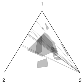
(a)

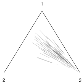
(b)

Figure 7: Up-projection of posterior samples $(\theta_{1},\theta_{2})$, obtained from $(N_{1}=8,N_{2}=4)$ and a Dirichlet(2,2) prior (segments in 7a), and feasible sets obtained independently for counts $(2,1,3)$ (polygons in 7a). The rule of combination retains non-empty intersections of these sets (7b).

4.3 Adding observations

We consider the addition of new observations to existing categories. Denote by $\mathbf{x}_{N+1}$ the original data $\mathbf{x}_{N}$ augmented with an observation $x_{N+1}$, which we assume equal to $k\in[K]$.

Any $u_{1:N+1}\in\mathcal{R}_{\mathbf{x}_{N+1}}$ is such that $u_{1:N}\in\mathcal{R}_{\mathbf{x}_{N}}$ and $u_{N+1}\in\Delta_{k}(\theta)$, with $\theta\in\Delta$ constructed from $u_{1:N}$ as in Proposition 3.2. Indeed if $u_{1:N+1}=(u_{1},\ldots,u_{N+1})\in\mathcal{R}_{\mathbf{x}_{N+1}}$, there exists $\theta^{\prime}\in\Delta$ such that, for all $n\in[N+1]$, $u_{n,\ell}/u_{n,k}\geq\theta^{\prime}_{\ell}/\theta^{\prime}_{k}$. Thus $u_{1:N}\in\mathcal{R}_{\mathbf{x}_{N}}$. We can check that $u_{N+1}$ is in $\Delta_{k}(\theta)$. Since $u_{1:N+1}\in\mathcal{R}_{\mathbf{x}_{N+1}}$, then $(u_{n})_{n\in\mathcal{I}_{k}}$ belongs to the support of $\nu_{\mathbf{x}_{N+1}}(d\mathbf{u}_{\mathcal{I}_{k}}|\mathbf{u}_{[N+1]\setminus\mathcal{I}_{k}})$, which is $\Delta_{k}(\theta)^{N_{k}}$ by Proposition 3.2. Here we have re-defined $\mathcal{I}_{k}=\{n\in[N+1]:x_{n}=k\}$. Conversely, if $u_{1:N}\in\mathcal{R}_{\mathbf{x}_{N}}$ and $u_{N+1}\in\Delta_{k}(\theta)$ then $u_{1:N+1}\in\mathcal{R}_{\mathbf{x}_{N+1}}$; again because $\Delta_{k}(\theta)$ is precisely the support of $\nu_{\mathbf{x}_{N+1}}(du_{N+1}|\mathbf{u}_{[N+1]\setminus\mathcal{I}_{k}})$.

This motivates an importance sampling strategy. For $u_{1:N}\sim\nu_{\mathbf{x}_{N}}$, generate $u_{N+1}\sim\Delta_{k}(\theta)$, with $\theta\in\Delta$ as above. Denote this distribution by $q_{N+1}(du_{N+1}|u_{1:N})$. The density $u_{N+1}\mapsto q_{N+1}(u_{N+1}|u_{1:N})$ equals $(\theta_{k})^{-1}$ for $u_{N+1}\in\Delta_{k}(\theta)$, since the volume of $\Delta_{k}(\theta)$ is $\theta_{k}$. We can correct for the discrepancy between proposal and target by computing weights

$$w_{N+1}(u_{1:N+1})=\frac{\nu_{\mathbf{x}_{N+1}}(u_{1:N+1})}{\nu_{\mathbf{x}_{N}}(u_{1:N})q_{N+1}(u_{N+1}|u_{1:N})} =\frac{Z_{N}}{Z_{N+1}}\text{Vol}(\Delta_{k}(\theta)),$$

where $Z_{N}$ is the volume of $\mathcal{R}_{\mathbf{x}_{N}}$. We can thus implement self-normalized importance sampling (Owen, 2013). The reasoning can be extended to assimilate observations recursively with a sequential Monte Carlo sampler (Del Moral et al., 2006), alternating importance sampling and Gibbs moves. This strategy will be employed in Section 5.1.

5 Applications

We present two applications. In both examples, the $(\texttt{p},\texttt{q},\texttt{r})$ probabilities require distributional information about the entire random polytopes, and not only the extreme vertices elicited in Dempster (1972). Both examples involve $K=4$ categories and curves in the simplex shown in Figure 8. Our main objective is to illustrate the output of the algorithm. We briefly recall from Section 2 that the inferred p and q probabilities can be understood as the degree of evidential support “for” or “against” the hypothesis of interest based on available observations and the model specification. The r probability, which is a distinctive feature of DS compared to standard Bayes, indicates a degree of epistemological indeterminacy, with a larger value encouraging the analyst to suspend judgment about the assertion of interest. The r probability can be useful to make decisions or to postpone them, as with other types of imprecise probabilities and robust Bayesian analysis (Berger et al., 1994). The way that decisions can be informed by DS uncertainties has received some attention, for example see Section 12 of Shafer (1990), and also Yager (1992); Bauer (1997).

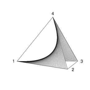
(a)

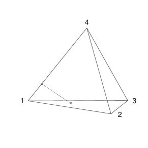
(b)

Figure 8: Two surfaces in the 4-simplex. 8a shows the independence surface $\theta_{1}\theta_{4}=\theta_{2}\theta_{3}$ (Fienberg and Gilbert, 1970). 8b shows the linkage constraint of (5.1) for $\phi\in(0,1)$ as a dashed segment.

5.1 Testing independence

In the case of $K=4$, count data may be arranged in a $2\times 2$ table with proportions $(\theta_{1},\theta_{2},\theta_{3},\theta_{4})$ as cell probabilities, row by row. We may be interested in testing independence, $H_{0}:\theta_{1}\theta_{4}=\theta_{2}\theta_{3}$, see Wasserman (Chapter 15, 2013). Classic tests include the Pearson’s chi-squared test with $\chi^{2}=\sum_{i,j}{(x_{ij}-e_{ij})^{2}}/{e_{ij}}$, where $e_{ij}$ is the expected number of counts in cell “$ij$” under $H_{0}$. The Pearson test statistic is asymptotically $\chi^{2}_{1}$. The likelihood ratio test with statistic $G^{2}=2\sum_{i,j}x_{ij}\log(x_{ij}/e_{ij})$, is asymptotically equivalent; see Diaconis and Efron (1985) for further interpretations.

Evaluating the posterior probability of $H_{0}$ raises the issue that the set $\{\theta\in\Delta\colon\theta_{1}\theta_{4}=\theta_{2}\theta_{3}\}$, a surface in the 4-simplex as depicted in Figure 8a, might be of zero measure under the posterior. As a remedy one can employ Bayes factors (e.g. Albert and Gupta, 1983), or we can consider the evidence towards either positive or negative association, i.e. $H_{+}:\theta_{1}\theta_{4}\geq\theta_{2}\theta_{3}$ or $H_{-}:\theta_{1}\theta_{4}\leq\theta_{2}\theta_{3}$, and interpret such evidence as being against independence.

We consider the data set presented in Rosenbaum (2002, p.191) regarding the effect of drainage pits on incident survival in the London underground. Some stations are equipped with drainage pits below the tracks. Passengers who accidentally fall off the platform may seek refuge in the pit to avoid an incoming train. For stations without a pit, only 5 lived out of 21 recorded incidents. In the presence of a pit, 18 out of 32 lived. Ding and Miratrix (2019) reanalyzed the data to assess the difference in mortality rates. Their analysis suggests that the existence of a pit significantly increases the chance of survival. The data can be summarized as counts $(16,5,14,18)$. Pearson’s chi-squared test statistic is $\chi^{2}=5.43$ with a p-value of $0.02$, while the likelihood ratio test yields a p-value of $0.017$. The Bayesian analysis shows strong evidence for positive association, with posterior probabilities ${P}(H_{+}\mid{\bf x})=0.99$ and ${P}(H_{-}\mid{\bf x})=0.01$.

The DS approach applied sequentially yields the results shown in Figure 9. The horizontal axis shows the observations, in an arbitrary order. The dark ribbon tracks $\texttt{p}(H_{+})$ and $(1-\texttt{q}(H_{+}))$ by its lower and upper rims, respectively. The “don’t know” probability $\texttt{r}(H_{+})$, represented by the width of the ribbon, can be seen to progressively shrink, but not systematically. The support for $H_{+}$ increases with each observation in $\{1,4\}$ and decreases with each observation in $\{2,3\}$ (as highlighted with background shades). Figure 9 is inspired by Figure 4 of Walley et al. (1996). In DS inference, the width of the ribbon is part of the inference and could be used, for example, to inform decisions about the collection of additional data.

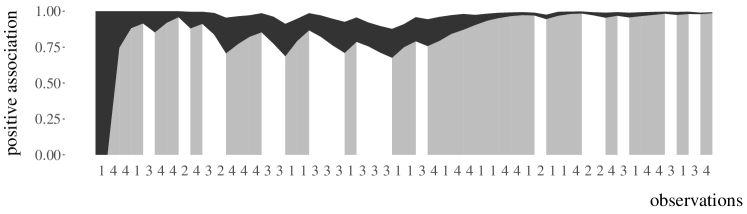
Figure 9: Support for the hypothesis of positive association $H_{+}:\theta_{1}\theta_{4}\geq\theta_{2}\theta_{3}$ as observations in $\{1,2,3,4\}$ are incorporated one by one. The dark ribbon delineates the probability p for $H_{+}$, and one minus the support against it, respectively as its lower and upper rims. The width of the ribbon represents the amount of “don’t know” about the hypothesis.

5.2 Linkage model

The linkage model from Rao (1973, pp.368-369) was considered by Lawrence et al. (2009), as an example illustrating inference with an additional constraint. They compare the Imprecise Dirichlet Model (IDM) of Walley (1996) and their method termed Dirichlet DSM (for Dempster–Shafer Model). The data consist of $N=197$ counts over $K=4$ categories, with probabilities satisfying

$${\theta}(\phi)=\left(\frac{1}{2}+\frac{\phi}{4},\frac{1-\phi}{4},\frac{1-\phi}{4},\frac{\phi}{4}\right),$$ (5.1)

for some $\phi\in(0,1)$. In other words, $\theta(\phi)=A\phi+b$ for appropriately defined $4\times 1$ matrices $A$ and $b$, as shown in Figure 8b. The original observations were $(125,18,20,34)$, but Lawrence et al. (2009) considered the counts $(25,3,4,7)$, which results in a more visible amount of “don’t know” probability.

We briefly introduce Dirichlet DSM and focus on the comparison between the approaches. They differ by the choice of sampling mechanism: instead of using the mechanism described in Dempster (1966), Lawrence et al. (2009) introduced another mechanism in order to make inference simpler computationally. For a vector of counts $\left(N_{1},...,N_{K}\right)$, the Dirichlet DSM model expresses its posterior inference for the proportion vector ${\theta}$ via the random feasible set $\{{\theta}\in\Delta:\theta_{1}\geq z_{1},...,\theta_{K}\geq z_{K}\},$ where ${\bf z}=\left(z_{0},z_{1},...,z_{K}\right)\sim\text{Dirichlet}_{K+1}(1,N_{1},...,N_{K})$. Incorporating the parameter constraint $\theta=A\phi+b$, the feasible set for $\phi$ is $[\phi_{\min}({\bf z}),\phi_{\max}({\bf z})]$ with

$$\phi_{\min}({\bf z})\equiv\max\left(4z_{1}-2,4z_{4}\right)\leq\phi_{\max}({\bf z})\equiv\min\left(1-4z_{2},1-4z_{3}\right).$$ (5.2)

For the approach of Dempster (1966), termed “Simplex-DSM” in Lawrence et al. (2009), we first run the proposed Gibbs sampler without taking into account the linear constraint (5.1). Among the generated feasible sets, only those that intersect with the linear constraint are retained, and an interval $[\underline{\phi},\overline{\phi}]$ is obtained for each such set, where

$$\underline{\phi}=\text{argmin}_{\phi}\left\{\theta\left(\phi\right)\in\mathcal{F}\left({\bf u}\right)\right\},\qquad\overline{\phi}=\text{argmax}_{\phi}\left\{\theta\left(\phi\right)\in\mathcal{F}\left({\bf u}\right)\right\}.$$

For the data considered here, this retains $5\%$ of the iterations, and is therefore a practical solution. However the approach would become impractical if the counts were much less “compatible” with the linkage constraint, in which case novel computational methods would be necessary. We estimate $(\texttt{p},\texttt{q},\texttt{r})$ for sets $\{\phi\in[0,c)\}$ for $c\in(0,1)$, i.e. lower and upper cumulative distribution functions, under both approaches and represent them in Figure 10a. The plot shows the overall agreement between the two approaches. Figure 10b highlights the difference in r values, and illustrates that multiple approaches within the DS framework lead to different results.

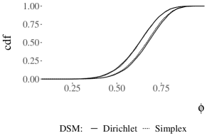
(a)

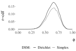
(b)

Figure 10: “Dirichlet-DSM” approach of Lawrence et al. (2009) and the original approach of Dempster (1966), for the linkage model with data $(25,3,4,7)$, the latter implemented with the proposed Gibbs sampler. Here 10a shows the lower and upper probabilities for assertions of the form $\{\phi<c\}$ for increasing $c\in[0,1]$, while 10b depicts the difference between these upper and lower probabilites, or equivalently the r values.

6 Discussion

The discipline of statistics does not have a single framework for parameter inference. The setting of count data is rich enough to contrast various approaches. Before any other considerations, for a framework to be useful to scientists and decision-makers, the ability to perform the associated computation is essential, and allows for grounded discussions and concrete comparisons. Our work helps with the computation in the DS framework for Categorical distributions, which will hopefully motivate further theoretical investigations of its statistical features.

One of the appeals of the DS framework is its flexibility to incorporate types of partial information which are difficult to express in the Bayesian framework. This includes vacuous or partial priors, coarse data which arise from imprecise measurement devices and imperfect surveys. These elements can be represented as random sets (Nguyen, 2006; Plass et al., 2015) in the DS framework while circumventing assumptions about the coarsening mechanism (e.g. Heitjan and Rubin, 1991).

Whether a perfect sampler could be devised as an alternative to the proposed Gibbs sampler is an open question. Generic algorithms for uniform sampling on polytopes (Vempala, 2005; Narayanan, 2016; Chen et al., 2018) could also provide competitive results. The proposed Gibbs sampler could itself be accelerated, for instance by using warm starts in the linear program solvers over subsequent iterations.

The typical challenge of DS computations is the generation of non-empty intersections of random sets. The proposed Gibbs sampler can be seen as a way of avoiding inefficient rejection samplers in the setting of inference in Categorical distributions. It remains to see whether similar ideas can be used to deploy the DS framework in other models, for example to avoid rejection sampling in the linkage model, or in hidden Markov models and models with moment constraints (Chamberlain and Imbens, 2003; Bornn et al., 2019), which are natural extensions of the Categorical distribution.

Acknowledgements

The authors thank Rahul Mazumder for useful advice on linear programming. The plots were generated using ggplot2 (Wickham, 2016) and R (R Core Team, 2018). The authors gratefully acknowledge support from the National Science Foundation (DMS-1712872, DMS-1844695, DMS-1916002), and the National Institute of Allergy and Infectious Disease at the National Institutes of Health [2 R37 AI054165-11 and 75N93019C00070]. The content is solely the responsibility of the authors and does not necessarily represent the official views of the National Institutes of Health.

Appendix A The choice of sampling mechanism

In DS inference, the sampling mechanism of the observable data is defined by a structural equation which deterministically associates the data $x$ with the parameter $\theta$ and an auxiliary random variable $u$, of an appropriate dimension and a known distribution. Inference for $\theta$ is obtained by inverting the structural equation and fixing $x$ at its observed value, resulting in a map from $u$ to subsets of the parameter space. In the present work, we have denoted this map as $\mathcal{F}$, suppressing its dependence on $x$.

Different sampling mechanisms may result in different DS inference for the parameter $\theta$, even if both mechanisms correspond to the same likelihood of the data $x$ as a function of $\theta$. We give an example in the case $K=2$, and consider two sampling mechanisms corresponding to $x\sim\text{Binomial}(N,\theta)$, where $\theta\in[0,1]$. The first sampling mechanism is essentially the same as that described in the main text, but adapted to the case where $K=2$. We define $u$ as an $N$-vector $(u_{1},\ldots,u_{N})$ of independent Uniform$(0,1)$ variables, and the structural equation

$$x=\sum_{n=1}^{N}{\mathds{1}}\left(u_{n}\leq\theta\right).$$ (A.1)

Upon observing $x$, inverting the equation gives a map from $(u_{1},\ldots,u_{N})\in[0,1]^{N}$ to measurable subsets of $[0,1]$. The random sets are of the form $[u_{\left(x\right)},u_{\left(x+1\right)}]$, random closed intervals with end points given by the $x$-th and $x+1$-th order statistics of $u_{1},\ldots,u_{N}$, with the convention $u_{(0)}=0,u_{(N+1)}=1$.

The second sampling mechanism amounts to an inverse transform method applied to the Binomial distribution, and involves the quantile function $Q_{a,b}$ of the $\text{Beta}(a,b)$ distribution. Consider the equation

$$x=\sum_{n=0}^{N-1}\mathds{1}\left(Q_{n+1,N-n}\left(u\right)\leq\theta\right),$$ (A.2)

where $u\sim\text{Uniform}(0,1)$. Using the fact that $(x,u)\mapsto Q_{x+1,N-x}(u)$ is increasing in $x$ for fixed $u$, it can be shown that $x$ follows a $\text{Binomial}(N,\theta)$. For fixed $x$, the random sets of interest are of the form

$$\left[Q_{x,N-x+1}\left(u\right),Q_{x+1,N-x}\left(u\right)\right],$$ (A.3)

and we observe that the endpoints are distributed marginally as the endpoints of $[u_{\left(x\right)},u_{\left(x+1\right)}]$, $\text{Beta}(x,N-x+1)$ and $\text{Beta}(x+1,N-x)$ respectively. The random interval of the form (A.3) is employed for Binomial inference by the Inferential Model framework [Martin and Liu, 2015, Section 9.3.4]. We observe from (A.3) that the length of these intervals is deterministic given either endpoint, which is not the case for the intervals of the form $[u_{\left(x\right)},u_{\left(x+1\right)}]$. Therefore the $(\texttt{p},\texttt{q},\texttt{r})$ triples associated with assertions of interest on the parameters are in general different.

Appendix B Sampling mechanism and Gumbel-max trick

We observe an equivalence between the mechanism to sample Categorical random variables from Dempster [1966] and the “Gumbel-max” trick [Maddison et al., 2014, 2016, Jang et al., 2016, Paulus et al., 2020].

As in the main text, we can sample from a Categorical distribution with parameters $\theta_{1},\ldots,\theta_{K}$ as follows: sample $w$ uniformly in the simplex $\Delta$, and output the integer $k\in[K]$ such that $w\in\Delta_{k}(\theta)$. To sample $w$ uniformly in $\Delta$, we can sample $\tilde{w}_{1},\ldots,\tilde{w}_{K}$ as independent Exponential(1), and normalize: the $\ell$-th component $w_{\ell}$ of $w$ is $\tilde{w}_{\ell}/\sum_{j\in[K]}\tilde{w}_{j}$. According to Lemma 5.2 in Dempster [1966], the output $k\in[K]$ is such that $w_{\ell}/w_{k}\geq\theta_{\ell}/\theta_{k}$ for all $\ell\in[K]$. Taking the logarithm and rearranging, this is equivalent to

$$\forall\ell\in[K]\quad\log\theta_{\ell}-\log\tilde{w}_{\ell}\leq\log\theta_{k}-\log\tilde{w}_{k}.$$

Since each $\tilde{w}_{\ell}$ is Exponential(1), $-\log\tilde{w}_{\ell}$ is a standard Gumbel. Therefore the procedure is equivalent to selecting

$$k=\text{argmax}_{\ell\in[K]}\log\theta_{\ell}+G_{\ell},$$

where $(G_{\ell})$ are independent Gumbel. This is exactly the “Gumbel-max trick”, see equation (2) in Maddison et al. [2014]. An appeal of that sampling mechanism is that the categories “are to be treated without regard to order” [Dempster, 1966], whereas the more common ways of sampling from a Categorical distribution involve ordering the categories. A similar appeal of the Gumbel-max trick is described in Oberst and Sontag [2019].

Appendix C Convergence rate when $K=2$

We consider the convergence of the proposed Gibbs sampler in the case of two categories, $K=2$. The analysis quantifies the impact of the counts $(N_{1},N_{2})$ on the convergence of the chain, which aligns with numerical experiments shown in the main text. In the case $K=2$ the Gibbs sampler is of course unnecessary, as we can sample the feasible sets simply by sorting Uniform draws, as described in Appendix A.

In the case $K=2$, $\Delta$ is the interval $[0,1]$ and the Gibbs sampler takes a particularly explicit form. We assume $N_{1}\geq 1,N_{2}\geq 1$. The conditional distributions of $u_{n},n\in\mathcal{I}_{k}$ given all $u_{n},n\in\mathcal{I}_{j}$ under $\nu_{\mathbf{x}}$ are

$$\nu_{\mathbf{x}}((u_{n})_{n\in\mathcal{I}_{1}}|(u_{n})_{n\in\mathcal{I}_{2}}) \propto\prod_{n\in\mathcal{I}_{1}}\mathds{1}(u_{n}\in(0,\min_{m\in\mathcal{I}_{2}}u_{m})),$$

$$\nu_{\mathbf{x}}((u_{n})_{n\in\mathcal{I}_{2}}|(u_{n})_{n\in\mathcal{I}_{1}}) \propto\prod_{n\in\mathcal{I}_{2}}\mathds{1}(u_{n}\in(\max_{m\in\mathcal{I}_{1}}u_{m},1)),$$

so that both conditionals are products of Uniform distributions. The variables $\max_{n\in\mathcal{I}_{1}}u_{n}$ and $\min_{n\in\mathcal{I}_{2}}u_{n}$ can be sampled from directly from translated and scaled Beta distributions. The Gibbs sampler alternatively updates these two variables, which we denote by $Y$ and $Z$ below. The procedure is described in Algorithm 3. Note that $Y^{(t)}\leq Z^{(t)}$ almost surely for all $t\geq 0$ and the feasible sets “$\mathcal{F}(\mathbf{u})$” are the intervals $[Y^{(t)},Z^{(t)}]$.

• Initialization: e.g. set $Y^{(0)}=1/2$, $Z^{(0)}=1/2$.

• At iteration $t\geq 1$,

  • Draw $Y^{(t)}=Z^{(t-1)}\times\text{Beta}(N_{1},1)$,

  • Draw $Z^{(t)}=Y^{(t)}+(1-Y^{(t)})\times\text{Beta}(1,N_{2})$.

• Output chain $(Y^{(t)},Z^{(t)})_{t\geq 0}$.

Algorithm 3 Gibbs sampler for the Bernoulli model, $K=2$.

We can re-write the evolution of $Z^{(t)}$ as

$$Z^{(t)}=B_{1}(1-B_{2})Z^{(t-1)}+B_{2},$$

where $B_{1}\sim\text{Beta}(N_{1},1)$ and $B_{2}\sim\text{Beta}(1,N_{2})$ are independent. Then we recognize that the chain $(Z^{(t)})$ is an auto-regressive process with random coefficients. We can analyze its rate of convergence with a coupling strategy. Introduce another chain $(\tilde{Z}^{(t)})$, started at stationarity and evolving with the same random input as $(Z^{(t)})$. Then we can write

$$\mathbb{E}\left[\left|Z^{(t)}-\tilde{Z}^{(t)}\right|\mid Z^{(t-1)},\tilde{Z}^{(t-1)}\right]=\mathbb{E}\left[B_{1}(1-B_{2})\right]\cdot|Z^{(t-1)}-\tilde{Z}^{(t-1)}|.$$

Since $B_{1}$ and $B_{2}$ are independent Beta distributions, by induction we can compute

$$\mathbb{E}\left[\left|Z^{(t)}-\tilde{Z}^{(t)}\right|\right]\leq\left(\frac{N_{1}}{N_{1}+1}\times\frac{N_{2}}{N_{2}+1}\right)^{t}\cdot\mathbb{E}\left[\left|Z^{(0)}-\tilde{Z}^{(0)}\right|\right].$$

Therefore the chains contract towards one another on average, at a rate that depends on $N_{1},N_{2}$. This leads to geometric convergence in the Wasserstein distance [e.g Theorem 2.1 in Gibbs, 2004]. Using manipulations, the inequality $\mathbb{E}[|Z^{(0)}-\tilde{Z}^{(0)}|]\leq 1$ and the inequality $\log(x)\leq x-1$ for all $x>0$, the Markov chain $(Z^{(t)})$ is less than $\epsilon$ from stationarity in the 1-Wasserstein distance, with $\epsilon\in(0,1)$, for all $t$ larger than

$$\frac{(N_{1}+1)(N_{2}+1)}{N_{1}+N_{2}+2}(-\log(\epsilon)).$$

The above is an upper bound on the $\epsilon$-mixing time of the chain. If both $N_{1}$ and $N_{2}$ increase proportionally to the sum $N=N_{1}+N_{2}$, the bound increases linearly in $N$, which is in agreement with figures in the main text. If $N_{1}$ is fixed while $N_{2}$ increases to infinity, the mixing time is upper bounded by a constant independent of $N$.

Appendix D Estimated convergence rate based on coupled chains

We provide a quick description of the method of Biswas et al. [2019] to obtain upper bounds on the distance between a chain and its limiting distribution, that can be estimated by Monte Carlo simulations. We consider the total variation distance, defined for two variables $X$ and $Y$ as

$$\|\mathcal{L}(X)-\mathcal{L}(Y)\|_{\text{TV}}=\frac{1}{2}\sup_{h:|h|\leq 1}|\mathbb{E}[h(X)-h(Y)]|.$$

The supremum is over functions $h$ bounded by one. Suppose that we can construct two chains $X^{(t)}$ and $Y^{(t)}$, evolving marginally according to a Markov kernel $P$, converging to a distribution of interest $\pi$, and such that $X^{(t)}=Y^{(t)}$ in distribution for all $t\geq 0$, while $X^{(t)}=Y^{(t-L)}$ almost surely for $t\geq\tau^{(L)}=\inf\{t:X^{(t)}=Y^{(t-L)}\}$ and where $L\geq 1$ is a user-chosen “lag” integer.

Then Jacob et al. [2020], Biswas et al. [2019] provide a set of assumptions under which, for any function $h$ bounded by one,

$$\int h(x)\pi(dx)-\mathbb{E}[h(X^{(t)})]=\mathbb{E}\left[\sum_{j=1}^{\lceil(\tau^{(L)}-L-t)/L\rceil}\left(h(X^{(t+jL)})-h(Y^{(t+(j-1)L)})\right)\right].$$

This comes from a telescopic sum argument first derived in the context of coupled Markov chains by Glynn and Rhee [2014]. From there, conditioning on $\tau^{(L)}$, taking triangle inequalities and upper bounding $|h(x)-h(y)|$ by $2$ for all $x,y$, we obtain

$$\|\mathcal{L}(X^{(t)})-\pi\|_{\text{TV}} \leq\mathbb{E}\left[\max(0,\lceil(\tau^{(L)}-L-t)/L\rceil)\right].$$

The right-hand side can be estimated by generating independent copies of $\tau^{(L)}$, in other words by sampling coupled Markov chains with a lag and recording their meeting time $\tau^{(L)}$, and then by approximating the expectation by an empirical average.

It remains to describe the coupling employed for the proposed Gibbs sampler. Denoting by $P$ the transition kernel of the Gibbs sampler, so that $\mathbf{u}^{\prime}\sim P(\mathbf{u},\cdot)$ given $\mathbf{u}\in\Delta^{N}$, we construct a coupled transition kernel $\bar{P}$ on $\Delta^{N}\times\Delta^{N}$. The second chain is denoted by $\tilde{\mathbf{u}}$. We employ the following coupling strategy. With probability $\omega\in(0,1)$, we propagate the two chains using common random numbers. As we have established in the case $K=2$ in Section C, this induces a contraction between the chains. With the remaining probability, conditional updates are maximally coupled [e.g Thorisson, 2000, Jacob et al., 2020], so that we have a chance to observe $\mathbf{u}^{(t)}=\tilde{\mathbf{u}}^{(t-L)}$. This mixture strategy is similar to that employed in Heng and Jacob [2019] for Hamiltonian Monte Carlo samplers. The mixing parameter $\omega$ was set to $0.9$ throughout our experiments.

For the choice of lag, we have used $L=50$ for Figure 5(a) in the main text and $L=10\times N$ for Figure 5(b), and both figures are obtained from $500$ independent copies of $\tau^{(L)}$, which took a few minutes to run on a personal computer from 2019 with a 2.4 GHz Intel Core i9, using 7 cores, 14 threads.

References

- Albert and Gupta [1983] J. H. Albert and A. K. Gupta. Bayesian estimation methods for 2 2 contingency tables using mixtures of Dirichlet distributions. Journal of the American Statistical Association, 78(383):708–717, 1983.
- Avis and Fukuda [1992] D. Avis and K. Fukuda. A pivoting algorithm for convex hulls and vertex enumeration of arrangements and polyhedra. Discrete & Computational Geometry, 8(3):295–313, 1992.
- Bang-Jensen and Gutin [2008] J. Bang-Jensen and G. Z. Gutin. Digraphs: theory, algorithms and applications. Springer Science & Business Media, 2008.
- Basir and Yuan [2007] O. Basir and X. Yuan. Engine fault diagnosis based on multi-sensor information fusion using Dempster–Shafer evidence theory. Information fusion, 8(4):379–386, 2007.
- Bauer [1997] M. Bauer. Approximation algorithms and decision making in the Dempster–Shafer theory of evidence - an empirical study. International Journal of Approximate Reasoning, 17(2-3):217–237, 1997.
- Berger and Bernardo [1992] J. O. Berger and J. M. Bernardo. Ordered group reference priors with application to the multinomial problem. Biometrika, 79(1):25–37, 1992.
- Berger et al. [1994] J. O. Berger, E. Moreno, L. R. Pericchi, M. J. Bayarri, J. M. Bernardo, J. A. Cano, J. De la Horra, J. Martín, D. Ríos-Insúa, and B. Betrò. An overview of robust Bayesian analysis. Test, 3(1):5–124, 1994.
- Berkelaar et al. [2004] M. Berkelaar, K. Eikland, and P. Notebaert. lpsolve: Open source (mixed-integer) linear programming system. Eindhoven U. of Technology, 63, 2004.
- Bernard [1998] J.-M. Bernard. Bayesian inference for categorized data. New ways in statistical methodology, pages 159–226, 1998.
- Biswas et al. [2019] N. Biswas, P. E. Jacob, and P. Vanetti. Estimating convergence of Markov chains with L-lag couplings. In Advances in Neural Information Processing Systems, pages 7389–7399, 2019.
- Bloch [1996] I. Bloch. Some aspects of Dempster–Shafer evidence theory for classification of multi-modality medical images taking partial volume effect into account. Pattern Recognition Letters, 17(8):905–919, 1996.
- Bornn et al. [2019] L. Bornn, N. Shephard, and R. Solgi. Moment conditions and Bayesian non-parametrics. Journal of the Royal Statistical Society: Series B (Statistical Methodology), 81(1):5–43, 2019.
- Chafai and Concordet [2009] D. Chafai and D. Concordet. Confidence regions for the multinomial parameter with small sample size. Journal of the American Statistical Association, 104(487):1071–1079, 2009.
- Chamberlain and Imbens [2003] G. Chamberlain and G. W. Imbens. Nonparametric applications of Bayesian inference. Journal of Business & Economic Statistics, 21(1):12–18, 2003.
- Chen et al. [2018] Y. Chen, R. Dwivedi, M. J. Wainwright, and B. Yu. Fast MCMC sampling algorithms on polytopes. The Journal of Machine Learning Research, 19(1):2146–2231, 2018.
- Csardi and Nepusz [2006] G. Csardi and T. Nepusz. The igraph software package for complex network research. InterJournal, Complex Systems:1695, 2006. URL http://igraph.org.
- Dawid and Stone [1982] A. P. Dawid and M. Stone. The functional-model basis of fiducial inference. The Annals of Statistics, pages 1054–1067, 1982.
- Del Moral et al. [2006] P. Del Moral, A. Doucet, and A. Jasra. Sequential Monte Carlo samplers. Journal of the Royal Statistical Society: Series B (Statistical Methodology), 68(3):411–436, 2006.
- Dempster [1963] A. P. Dempster. On direct probabilities. Journal of the Royal Statistical Society: Series B (Methodological), pages 100–110, 1963.
- Dempster [1966] A. P. Dempster. New methods for reasoning towards posterior distributions based on sample data. The Annals of Mathematical Statistics, 37(2):355–374, 1966.
- Dempster [1967] A. P. Dempster. Upper and lower probabilities induced by a multivalued mapping. The Annals of Mathematical Statistics, 38(2):325–339, 1967.
- Dempster [1968] A. P. Dempster. A generalization of Bayesian inference. Journal of the Royal Statistical Society: Series B (Methodological), 30(2):205–247, 1968.
- Dempster [1972] A. P. Dempster. A class of random convex polytopes. The Annals of Mathematical Statistics, pages 260–272, 1972.
- Dempster [2008] A. P. Dempster. The Dempster–Shafer calculus for statisticians. International Journal of approximate reasoning, 48(2):365–377, 2008.
- Dempster [2014] A. P. Dempster. Statistical inference from a Dempster–Shafer perspective. In X. Lin, C. Genest, D. L. Banks, G. Molenberghs, D. W. Scott, and J.-L. Wang, editors, Past, Present, and Future of Statistical Science, pages 275–288. Chapman and Hall/CRC, 2014.
- Denoeux [2000] T. Denoeux. A neural network classifier based on Dempster–Shafer theory. IEEE Transactions on Systems, Man, and Cybernetics-Part A: Systems and Humans, 30(2):131–150, 2000.
- Denœux [2006] T. Denœux. Constructing belief functions from sample data using multinomial confidence regions. International Journal of Approximate Reasoning, 42(3):228–252, 2006.
- Denoeux [2008] T. Denoeux. A k-nearest neighbor classification rule based on Dempster–Shafer theory. In Classic works of the Dempster-Shafer theory of belief functions, pages 737–760. Springer, 2008.
- Diaconis and Efron [1985] P. Diaconis and B. Efron. Testing for independence in a two-way table: new interpretations of the chi-square statistic. The Annals of Statistics, pages 845–874, 1985.
- Díaz-Más et al. [2010] L. Díaz-Más, R. Muñoz-Salinas, F. J. Madrid-Cuevas, and R. Medina-Carnicer. Shape from silhouette using Dempster–Shafer theory. Pattern Recognition, 43(6):2119–2131, 2010.
- Ding and Miratrix [2019] P. Ding and L. W. Miratrix. Model-free causal inference of binary experimental data. Scandinavian Journal of Statistics, 46(1):200–214, 2019.
- Dunson and Xing [2009] D. B. Dunson and C. Xing. Nonparametric Bayes modeling of multivariate categorical data. Journal of the American Statistical Association, 104(487):1042–1051, 2009.
- Edlefsen et al. [2009] P. T. Edlefsen, C. Liu, and A. P. Dempster. Estimating limits from Poisson counting data using Dempster–Shafer analysis. The Annals of Applied Statistics, 3(2):764–790, 2009.
- Fienberg and Gilbert [1970] S. E. Fienberg and J. P. Gilbert. The geometry of a two by two contingency table. Journal of the American Statistical Association, 65(330):694–701, 1970.
- Fisher [1935] R. A. Fisher. The fiducial argument in statistical inference. Annals of eugenics, 6(4):391–398, 1935.
- Fitzpatrick and Scott [1987] S. Fitzpatrick and A. Scott. Quick simultaneous confidence intervals for multinomial proportions. Journal of the American Statistical Association, 82(399):875–878, 1987.
- Fraser [1968] D. A. S. Fraser. The Structure of Inference. New York: John Wiley and Sons, 1968.
- Fukuda [1997] K. Fukuda. cdd/cdd+ reference manual. Institute for Operations Research, ETH-Zentrum, pages 91–111, 1997.
- Geyer and Meeden [2008] C. J. Geyer and G. D. Meeden. R package rcdd (C double description for R), version 1.1, 2008.
- Gibbs [2004] A. L. Gibbs. Convergence in the Wasserstein metric for Markov chain Monte Carlo algorithms with applications to image restoration. Stochastic Models, 20(4):473–492, 2004. doi: 10.1081/STM-200033117.
- Glynn and Rhee [2014] P. W. Glynn and C.-h. Rhee. Exact estimation for Markov chain equilibrium expectations. Journal of Applied Probability, 51(A):377–389, 2014.
- Gong [2018] R. Gong. Low-resolution Statistical Modeling with Belief Functions. PhD thesis, Harvard University, 2018.
- Gong [2019] R. Gong. Simultaneous inference under the vacuous orientation assumption. Proceedings of Machine Learning Research, 103:225–234, 2019.
- Hannig et al. [2016] J. Hannig, H. Iyer, R. C. S. Lai, and T. C. M. Lee. Generalized fiducial inference: a review and new results. Journal of the American Statistical Association, 111(515):1346–1361, 2016.
- Heitjan and Rubin [1991] D. F. Heitjan and D. B. Rubin. Ignorability and coarse data. The Annals of Statistics, pages 2244–2253, 1991.
- Heng and Jacob [2019] J. Heng and P. E. Jacob. Unbiased Hamiltonian Monte Carlo with couplings. Biometrika, 106(2):287–302, 2019.
- Jacob et al. [2020] P. E. Jacob, J. O’Leary, and Y. F. Atchadé. Unbiased Markov chain Monte Carlo methods with couplings. Journal of the Royal Statistical Society: Series B (Statistical Methodology), 82(3):543–600, 2020.
- Jang et al. [2016] E. Jang, S. Gu, and B. Poole. Categorical reparameterization with Gumbel-softmax. arXiv preprint arXiv:1611.01144, 2016.
- Jerrum [1998] M. Jerrum. Mathematical foundations of the Markov chain Monte Carlo method. In Probabilistic methods for algorithmic discrete mathematics, pages 116–165. Springer, 1998.
- Konis [2014] K. Konis. lpSolveAPI: R interface for lpsolve version 5.5. R package version, 5:2–0, 2014.
- Lang [2004] J. B. Lang. Multinomial-Poisson homogeneous models for contingency tables. The Annals of Statistics, 32(1):340–383, 2004.
- Lawrence et al. [2009] E. C. Lawrence, S. Vander Wiel, C. Liu, and J. Zhang. A new method for multinomial inference using Dempster-Shafer theory. Technical report, Los Alamos National Lab, Los Alamos, New Mexico, United States, 2009.
- Liu [2000] C. Liu. Estimation of discrete distributions with a class of simplex constraints. Journal of the American Statistical Association, 95(449):109–120, 2000.
- Liu and Hannig [2016] Y. Liu and J. Hannig. Generalized fiducial inference for binary logistic item response models. Psychometrika, 81(2):290–324, 2016.
- Maddison et al. [2014] C. J. Maddison, D. Tarlow, and T. Minka. A* sampling. In Advances in Neural Information Processing Systems, pages 3086–3094, 2014.
- Maddison et al. [2016] C. J. Maddison, A. Mnih, and Y. W. Teh. The concrete distribution: A continuous relaxation of discrete random variables. arXiv preprint arXiv:1611.00712, 2016.
- Martin and Liu [2015] R. Martin and C. Liu. Inferential models: reasoning with uncertainty, volume 145. CRC Press, 2015.
- Narayanan [2016] H. Narayanan. Randomized interior point methods for sampling and optimization. The Annals of Applied Probability, 26(1):597–641, 2016.
- Nguyen [2006] H. T. Nguyen. An introduction to random sets. CRC Press, Boca Raton, FL, 2006.
- Oberst and Sontag [2019] M. Oberst and D. Sontag. Counterfactual off-policy evaluation with Gumbel-max structural causal models. arXiv preprint arXiv:1905.05824, 2019.
- Owen [2013] A. B. Owen. Monte Carlo theory, methods and examples. 2013.
- Paulus et al. [2020] M. B. Paulus, D. Choi, D. Tarlow, A. Krause, and C. J. Maddison. Gradient estimation with stochastic softmax tricks. arXiv preprint arXiv:2006.08063, 2020.
- Plass et al. [2015] J. Plass, T. Augustin, M. Cattaneo, and G. Schollmeyer. Statistical modelling under epistemic data imprecision: some results on estimating multinomial distributions and logistic regression for coarse categorical data. In ISIPTA, volume 15, pages 247–256, 2015.
- R Core Team [2018] R Core Team. R: A Language and Environment for Statistical Computing. R Foundation for Statistical Computing, Vienna, Austria, 2018. URL https://www.R-project.org/.
- Rao [1973] C. R. Rao. Linear statistical inference and its applications, volume 2. Wiley New York, 1973.
- Roberts and Rosenthal [2004] G. O. Roberts and J. S. Rosenthal. General state space Markov chains and MCMC algorithms. Probability surveys, 1:20–71, 2004.
- Rosenbaum [2002] P. R. Rosenbaum. Observational Studies. Springer-Verlag New York, 2002.
- Shafer [1976] G. Shafer. A mathematical theory of evidence, volume 42. Princeton university press, 1976.
- Shafer [1979] G. Shafer. Allocations of probability. The Annals of Probability, 7(5):827–839, 1979.
- Shafer [1990] G. Shafer. Perspectives on the theory and practice of belief functions. International Journal of Approximate Reasoning, 4(5-6):323–362, 1990.
- Sison and Glaz [1995] C. P. Sison and J. Glaz. Simultaneous confidence intervals and sample size determination for multinomial proportions. Journal of the American Statistical Association, 90(429):366–369, 1995.
- Thorisson [2000] H. Thorisson. Coupling, stationarity, and regeneration, volume 14. Springer New York, 2000.
- Vasseur et al. [1999] P. Vasseur, C. Pégard, E. Mouaddib, and L. Delahoche. Perceptual organization approach based on Dempster–Shafer theory. Pattern recognition, 32(8):1449–1462, 1999.
- Vempala [2005] S. Vempala. Geometric random walks: a survey. Combinatorial and computational geometry, 52(573-612):2, 2005.
- Walley [1996] P. Walley. Inferences from multinomial data: learning about a bag of marbles. Journal of the Royal Statistical Society: Series B (Statistical Methodology), 58(1):3–34, 1996.
- Walley et al. [1996] P. Walley, L. Gurrin, and P. Burton. Analysis of clinical data using imprecise prior probabilities. Journal of the Royal Statistical Society: Series D (The Statistician), 45(4):457–485, 1996.
- Wasserman [1990] L. Wasserman. Belief functions and statistical inference. Canadian Journal of Statistics, 18(3):183–196, 1990.
- Wasserman [2013] L. Wasserman. All of statistics: a concise course in statistical inference. Springer Science & Business Media, 2013.
- Wickham [2016] H. Wickham. ggplot2: Elegant Graphics for Data Analysis. Springer-Verlag New York, 2016. ISBN 978-3-319-24277-4. URL https://ggplot2.tidyverse.org.
- Yager [1992] R. R. Yager. Decision making under Dempster–Shafer uncertainties. International Journal of General System, 20(3):233–245, 1992.