Low-Resource Domain Adaptation for Speaker Recognition Using Cycle-GANs

Abstract

Current speaker recognition technology provides great performance with the x-vector approach. However, performance decreases when the evaluation domain is different from the training domain, an issue usually addressed with domain adaptation approaches. Recently, unsupervised domain adaptation using cycle-consistent Generative Adversarial Networks (CycleGAN) has received a lot of attention. CycleGAN learn mappings between features of two domains given non-parallel data. We investigate their effectiveness in low resource scenario i.e. when limited amount of target domain data is available for adaptation, a case unexplored in previous works. We experiment with two adaptation tasks: microphone to telephone and a novel reverberant to clean adaptation with the end goal of improving speaker recognition performance. Number of speakers present in source and target domains are 7000 and 191 respectively. By adding noise to the target domain during CycleGAN training, we were able to achieve better performance compared to the adaptation system whose CycleGAN was trained on a larger target data. On reverberant to clean adaptation task, our models improved EER by 18.3% relative on VOiCES dataset compared to a system trained on clean data. They also slightly improved over the state-of-the-art Weighted Prediction Error (WPE) de-reverberation algorithm.

Index Terms—  Domain Adaptation, CycleGAN, Low Resource, Microphone-Telephone, Speaker Recognition

1 Introduction

Speaker recognition technology has made great progress in the last decade. The x-vector approach [1] is the current state-of-the-art in this field, providing superior performance in NIST SRE, Speakers In The Wild (SITW) [2] and VoxCeleb datasets [3]. x-vectors is a data-hungry approach, i.e., it requires a huge amount of labeled data ($\sim 10$k speakers with multiple recordings per speaker) to be properly trained. Most data available for training consists of English speech of moderately good quality. When we apply x-vector networks trained on these data to other acoustic domains, performance dramatically drops. We can witness this in the latest NIST SRE18 [4]. Acquiring labeled data from thousands of speakers of each domain would be very expensive or just unfeasible. However, in some cases, it is possible to get access to certain amount of data from the domain of interest denoted from now on as the target domain. Then, we can make use of domain adaptation techniques to adapt features or models trained on data from the source domain–the domain with plenty of training data– to the target domain or vice-versa. The final goal is to improve the performance on evaluation corpora sampled from the target domain.

In this paper, we are interested in the particular case of low-resource unsupervised domain adaptation. It is low-resource because we assume a limited amount of target domain (LT) data is available to train the adaptation system. Furthermore, it is unsupervised in two ways. First, we assume that the adaptation data doesn’t have any speaker labels. Second, we assume that we don’t have any paired data between source and target domains. By paired data, we mean, for example, the case where somebody records the same conversation through close-talk and far-field microphones at the same time. Then, we can use the matched pairs to learn mapping functions between domains. This setting is of interest to us because this opens up the possibility of maximally taking advantage of small development set found in real data, and not use simulated sets (as done commonly in practice).

Typically, we find two types of strategies for domain adaptation. The first one consist of adapting a model trained on the source domain to the target domain. The second one, which is the one we follow, consist of mapping the acoustic input features from the target domain back to the source domain. Thus, we can use the original source domain speaker recognition system without any changes.

For this unsupervised scenario, CycleGAN [5] is an effective solution. Training objective function for CycleGAN is a combination of reconstruction and adversarial losses [6]. CycleGAN was first proposed in computer vision literature for image-to-image translation with non-parallel data. In speech research, CycleGAN has been used for mapping noisy speech to clean speech, improving automatic speech recognition (ASR) trained on clean speech [7, 8], voice conversion [9, 10, 11], gender adaptation [12], and microphone to telephone (mic-tel) adaptation for speaker recognition [13].

All works cited above have demonstrated the capability of CycleGAN for unsupervised domain adaptation across wide range of tasks. However, they were trained on comparable amounts of source and target domain data. For example, in the noisy to clean adaptation work in [8], the same amount of data is used for both domains- target domain data is created by artificially adding noise to clean data. Also in [9], the authors create target domain data by augmenting real noisy data with data created by artificially adding noise to the source domain. In our previous work  [13], we improved the performance of the speaker recognition system trained on telephone corpus on Speakers In The Wild (SITW) [2], a microphone corpus. For that, we used development portion of SITW and the much larger VoxCeleb1 dataset [3] as the target domain data to learn the feature mapping function.

In this work, we experimented with mic-tel (as done in [13]) and a novel reverberant to clean speech (reverb-clean) adaptation tasks, both with the end goal of improving speaker recognition performance under the low-resource setting. For both tasks, CycleGANs were trained with data from  7000 speakers from the source domain and 191 speakers from the target domain. We observed that the low-resource setting limits the capability of CycleGAN to learn meaningful mappings between domains. The drop in performance can be attributed to the phenomenon of over-fitting or lack of sufficient variation between the domains. To overcome this disadvantage, we experimented with artificially adding noise to the LT data before training CycleGAN. The motivation behind adding noise is to prevent over-fitting by making it act as a regularizer and to make both the source and target distributions more different (telephone corpus is often considered as clean) of which the adversarial loss can take advantage. By adding noise, adaptation system with CycleGAN trained on LT data performed slightly better than adaptation system whose CycleGAN was trained on larger amounts of target domain data. We observed this on both the tasks. More importantly, we observed that noise addition speeds up training (slightly better performance with fewer epochs of training). For the reverb-clean task, CycleGAN trained with LT data and added noise yielded good improvements (18.3% relative improvement in EER) w.r.t the baseline speaker recognition system trained on clean and tested on reverberant speech. CycleGAN adaptation also showed slight improvements over the state-of-the-art weighted prediction error (WPE) [14] de-reverberation algorithm.

2 Low-resource CycleGAN System

The adaptation procedure in this study is as follows. We start-off by training an x-vector network [1] on source domain data. During the evaluation, we map the input features of the x-vector network from target domain data to the source domain. This is accomplished by learning feature mapping functions between the two domains. The training corpora to learn the feature mapping functions consists of audio samples $\mathbf{A}_{\mathrm{S}}=\{{\mathbf{a}}_{\mathrm{S},i}\}_{i=1}^{N}$ and $\mathbf{A}_{\mathrm{T}}=\{{\mathbf{a}}_{\mathrm{T},i}\}_{i=1}^{M}$ drawn from two different domains: source $S$ and target $T$ with distributions ${\mathbf{a}}_{\mathrm{S},i}\sim q_{\mathrm{S}}({\mathbf{a}})$ and ${\mathbf{a}}_{\mathrm{T},i}\sim q_{\mathrm{T}}({\mathbf{a}})$ respectively. In this work we assume $M<<N$. Noise is then added to the target domain audio samples which result in a transformed target domain distribution $T^{\prime}$. Log mel-filter bank features are extracted from audio samples of source and transformed target domain distributions denoted as $\mathbf{X}_{\mathrm{S}}=\{\mathbf{x}_{\mathrm{S},i}\}_{i=1}^{N}$ and $\mathbf{X}_{\mathrm{T}^{\prime}}=\{\mathbf{x}_{\mathrm{T}^{\prime},i}\}_{i=1}^{M}$. The distributions in filter bank space are $\mathbf{x}_{\mathrm{S},i}\sim p_{\mathrm{S}}(\mathbf{x})$ and $\mathbf{x}_{\mathrm{T}^{\prime},i}\sim p_{\mathrm{T}^{\prime}}(\mathbf{x})$ respectively. $\mathbf{X}_{\mathrm{S}}$ and $\mathbf{X}_{\mathrm{T}^{\prime}}$ are used as features from two different distributions to train the feature mapping functions. Speaker labels from either domain are not needed to train the feature mapping function. The training data is assumed non-parallel which makes the adaptation procedure unsupervised. Noise is added to the target domain audio only during training. During evaluation original audio samples of the evaluation data sampled from the target domain data are used to extract filter bank features which are then mapped to the source domain. The target domain data used to train and evaluate the feature mapping system has no speaker overlap.

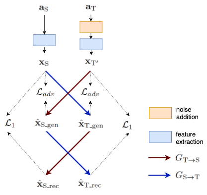
Fig. 1: CycleGAN layout

The feature mapping between domains is achieved by training a CycleGAN system. The training procedure for CycleGAN with LT data is outlined in Figure 1. It consists of two generators, each of which maps features of one domain to the opposite. It also has two discriminators, one for each domain (not shown in Figure 1). Each discriminator tries to distinguish between real features from its domain and features mapped (generated) from the opposite domain to that domain.

2.1 CycleGAN training objectives

The training procedure is as follows: two batches of features $\mathbf{x}_{\mathrm{S}}$ and $\mathbf{x}_{\mathrm{T}^{\prime}}$ are sampled from source and transformed target domains respectively. The generator $G_{\mathrm{T}\rightarrow\mathrm{S}}$ maps $\mathbf{x}_{\mathrm{T}^{\prime}}$ to source domain, producing features $\hat{\mathbf{x}}_{\mathrm{S}\_\mathrm{gen}}$. A discriminator $D_{\mathrm{S}}$ is trained to discriminate between original and generated source domain features. The generator $G_{\mathrm{T}\rightarrow\mathrm{S}}$ is then trained to output features $\hat{\mathbf{x}}_{\mathrm{S}\_\mathrm{gen}}$ that appear identical to the original target domain features $\mathbf{x}_{\mathrm{S}}$. This is accomplished by training the generator with an adversarial loss [6]. As recommended in [15], we used the least-squares objective to train our generator and discriminator (LS-GAN). $D_{\mathrm{S}}$ and $G_{\mathrm{T}\rightarrow\mathrm{S}}$ are trained to minimize the objectives 2.1 and 2 respectively.

$$L_{\mathrm{disc}}(G_{\mathrm{T}\rightarrow\mathrm{S}},D_{\mathrm{S}},\mathbf{X}_{\mathrm{T}^{\prime}},\mathbf{X}_{\mathrm{S}})= \mathop{\mathbb{E}_{\mathbf{x}\sim p_{\mathrm{T}^{\prime}}}[D_{\mathrm{S}}(G_{\mathrm{T}\rightarrow\mathrm{S}}(\mathbf{x}))^{2}]}+$$

$$\mathop{\mathbb{E}_{\mathbf{x}\sim p_{\mathrm{S}}}[(D_{\mathrm{S}}(\mathbf{x})-1)^{2}]}$$ (1)

$$L_{\mathrm{adv}}(G_{\mathrm{T}\rightarrow\mathrm{S}},D_{\mathrm{S}},\mathbf{X}_{\mathrm{T}^{\prime}})=\mathop{\mathbb{E}_{\mathbf{x}\sim p_{\mathrm{T}^{\prime}}}[(D_{\mathrm{S}}(G_{\mathrm{T}\rightarrow\mathrm{S}}(\mathbf{x}))-1)^{2}]}$$ (2)

Equivalently, the other generator-discriminator ($G_{\mathrm{S}\rightarrow\mathrm{T}}$, $D_{\mathrm{T}}$) pair is trained in a similar fashion to transfer features from source domain to transformed target domain. During evaluation, since we map features from the target domain to the source domain without adding noise, we keep the notation of generators as $G_{\mathrm{T}\rightarrow\mathrm{S}}$ instead of $G_{\mathrm{T}^{\prime}\rightarrow\mathrm{S}}$.

A single generator-discriminator pair trained with adversarial loss would suffice, in theory, to transfer features from one domain to the opposite domain. However, this leads to an ill-posed problem with adversarial loss putting a weak constraint on the generators. Thus, the generator could create many possible features which appear to be drawn from the true distribution but may fail to preserve the structure present in the signal like the linguistic information, speaker and gender information. To restrict the space of possible mappings from the generator, CycleGAN enforce cycle-consistency constraint on the generators - reconstructing the original features, e.g. $\mathbf{x}_{\mathrm{S}}$, from the generated features in the opposite domain, e.g., $\hat{\mathbf{x}}_{\mathrm{T}\_\mathrm{gen}}$. This is achieved by minimizing the objective in (3) between $\mathbf{x}_{\mathrm{S}}$ and $\hat{\mathbf{x}}_{\mathrm{S}\_\mathrm{rec}}=G_{\mathrm{T}\rightarrow\mathrm{S}}(\hat{\mathbf{x}}_{\mathrm{T}\_\mathrm{gen}})$ where we used $l_{1}$ distance as the metric. We refer to this loss as forward cycle consistency loss. Similarly, the loss computed between $\mathbf{x}_{\mathrm{T}^{\prime}}$ and $\hat{\mathbf{x}}_{\mathrm{T}\_\mathrm{rec}}$ is referred to as backward cycle consistency loss. The final cycle consistency loss is the combination of both these objectives and is given in (2.1).

$$L_{1}(G_{\mathrm{S}\rightarrow\mathrm{T}},G_{\mathrm{T}\rightarrow\mathrm{S}},\mathbf{X}_{\mathrm{S}})=\mathop{\mathbb{E}_{\mathbf{x}\sim p_{\mathrm{S}}}{||G_{\mathrm{T}\rightarrow\mathrm{S}}(G_{\mathrm{S}\rightarrow\mathrm{T}}(\mathbf{x}))-\mathbf{x}||}_{1}}$$ (3)

$$L_{\mathrm{cyc}}(G_{\mathrm{S}\rightarrow\mathrm{T}},G_{\mathrm{T}\rightarrow\mathrm{S}},\mathbf{X}_{\mathrm{S}},\mathbf{X}_{\mathrm{T}^{\prime}}) =L_{1}(G_{\mathrm{S}\rightarrow\mathrm{T}},G_{\mathrm{T}\rightarrow\mathrm{S}},\mathbf{X}_{\mathrm{S}})$$

$$+L_{1}(G_{\mathrm{T}\rightarrow\mathrm{S}},G_{\mathrm{S}\rightarrow\mathrm{T}},\mathbf{X}_{\mathrm{T}^{\prime}})$$ (4)

Finally, both the generators of CycleGAN are trained using multi-task objective: by minimizing both the adversarial and cycle consistency objectives as shown in (2.1). ${\lambda}_{\mathrm{cyc}}$ and ${\lambda}_{\mathrm{adv}}$ in (2.1) denote the weights assigned to cycle consistency loss and adversarial loss respectively.

$$L(G_{\mathrm{T}\rightarrow\mathrm{S}},G_{\mathrm{S}\rightarrow\mathrm{T}},D_{\mathrm{T}},D_{\mathrm{S}},\mathbf{X}_{\mathrm{S}},\mathbf{X}_{\mathrm{T}^{\prime}})$$

$$={\lambda}_{adv}L_{\mathrm{adv}}(G_{\mathrm{T}\rightarrow\mathrm{S}},D_{\mathrm{S}},\mathbf{X}_{\mathrm{T}^{\prime}})$$

$$+{\lambda}_{\mathrm{adv}}L_{\mathrm{adv}}(G_{\mathrm{S}\rightarrow\mathrm{T}},D_{\mathrm{T}},\mathbf{X}_{\mathrm{S}})$$

$$+{\lambda}_{\mathrm{cyc}}L_{\mathrm{cyc}}(G_{\mathrm{S}\rightarrow\mathrm{T}},G_{\mathrm{T}\rightarrow\mathrm{S}},\mathbf{X}_{\mathrm{S}},\mathbf{X}_{\mathrm{T}^{\prime}})$$ (5)

Table 1: Generator architecture

Layer	Kernel size	Output
Shortcut	-	h x w x 1
Downsampler
Conv, ReLU	[3,3,1]	h x w x 32
Conv, IN, ReLU	[3,3,2]	h/2 x w/2 x 64
Conv, IN, ReLU	[3,3,2]	h/4 x w/4 x 128
(ResBlock, ReLU) x 9	-	h/4 x w/4 x 128
Upsampler
Deconv, IN, ReLU	[3,3,2]	h/2 x w/2 x 64
Deconv, IN, ReLU	[3,3,2]	h x w x 32
Conv	[3,3,1]	h x w x 1
Addition	-	h x w x 1

Table 2: ResBlock architecture

Layer	Kernel size	Output
Shortcut	-	h/4 x w/4 x 128
Conv, IN, ReLU	[3,3,1]	h/4 x w/4 x 128
Conv, IN	[3,3,1]	h/4 x w/4 x 128
Addition	-	h/4 x w/4 x 128

Table 3: Discriminator architecture

Layer	Kernel size	Output
Conv, LeReLU	[4,4,2]	h/2 x w/2 x 64
Conv, LeReLU	[4,4,2]	h/4 x w/4 x 128
Conv, LeReLU	[4,4,2]	h/8 x w/8 x 256
Conv, LeReLU	[4,4,1]	h/8 x w/8 x 512
Conv	[4,4,1]	h/8 x w/8 x 1

2.2 Network architectures

The architecture for generators is given in Table 1. It is a full-convolutional network with a downsampler-upsampler architecture. Kernel size is described as [kernel_h, kernel_w, stride]. Input shape to the network is h x w and output shape of each layer is h x w x channels. Similar to the work in [13], we used a short cut connection from input and added the shortcut to the output of the last convolutional layer of the network. The architecture for the residual block used in the generator is given in Table 2 and the architecture for discriminators is given in Table 3. The slopes of all Leaky ReLU (LeReLU) functions were set to 0.2. Since we used least squares objective to train the discriminator, we have not applied any non-linear activation at the output. For both mic-tel and reverb-clean adaptation tasks, we used same network architectures and same training objectives

3 Experimental details for mic-tel adaptation

In this section, we describe the experimental setup for low-resource mic-tel adaptation.

3.1 source and target domain datasets

Telephone domain data (source domain) used to train x-vector system consisted of recordings from datasets SRE04-10, Mixer6 and Switchboard 1-Phase 1, 2, and 3. This gave us 90946 utterances from 6986 speakers. This was also used as the source domain data to train the CycleGAN system. Development corpus of SITW (referred to as SITW dev) was used as microphone corpus from the target domain to train the CycleGAN system. It has 4439 utterances from 119 speakers. The mismatch in the number of speakers and utterances between both the domains can clearly be observed justifying the need for low-resource domain adaptation. SITW evaluation corpus (referred to as SITW eval) was used to evaluate the system. No speaker overlap exists between SITW eval and dev corpora. The microphone speech was down-sampled to 8KHz to match the sampling frequency of telephone speech.

3.2 Noise addition to the target domain data

We added noise to the speech signals from the target domain to train CycleGAN. To add noise we used 930 ”noise” samples from MUSAN [16] corpus. Noise was added as foreground noises at the interval of 1 second with the signal to noise ratios (SNRs) ranging from 0 to 15dB. The ”music” and ”babble” portions of MUSAN corpus were not used in this work. Noise addition was done only on target domain data during the training of CycleGAN system. The original target domain data (without noise) was not used during training. While forward passing the SITW eval features through CycleGAN, no noise was added. No noise was added to the source domain data during the training of x-vector system and CycleGAN system.

3.3 Baseline system

The x-vector system was based on Kaldi [17]. We used the same setup as in SRE16 Kaldi recipe but without any data augmentation. The x-vector system was trained on telephone corpus mentioned in Section 3.1 and evaluated on SITW eval. The system used 40-dimensional log Mel filter-bank features with short-time centering (300 frames). Energy-based VAD was applied to remove the non-speech frames. x-vector network was trained for 3 epochs. After the training, the network was used to extract x-vectors (speaker embeddings) for the training and evaluation corpus. The x-vectors were centered, projected to 150 dimensions using Linear Discriminant Analysis (LDA) and length normalized. Full-rank Probabilistic Linear Discriminant Analysis (PLDA) [18] was used to get the scores. Finally, scores were normalized using adaptive symmetric norm (S-Norm) [19]. In the baseline system, both the x-vector network and PLDA backend were trained on telephone speech and tested on microphone speech.

3.4 Adaptation system

For the adaptation system, the x-vector network and PLDA were same as in the baseline. Feature adaptation was done in the evaluation stage. First, the filter-bank features of the evaluation corpus were mapped from microphone to telephone domain by forward passing through the $G_{\mathrm{T}\to\mathrm{S}}$ generator of CycleGAN network. Then, the mapped features were used to extract the x-vectors for the evaluation data.

3.5 CycleGAN training

Similar to x-vector system, CycleGAN system was trained on 40-dimensional log mel-filter bank features with short time centering. Energy VAD was applied on centered features to remove the non-speech frames. Two batches of features were sampled randomly from source and transformed target domain (target domain with noise) during each training step. Since no parallel data exists between both the domains, the batches were drawn in a completely random fashion. The size of the batches was set to 32 and the number of contiguous frames sampled from each utterance (sequence length) was set to 127. The model was trained for 50 epochs. Each epoch was set to be complete when all the telephone utterances have appeared once in that epoch. Adam Optimizer was used with momentum $\beta_{1}=0.5$ as suggested by [20]. The learning rates for the generators and discriminators were set to 0.0003 and 0.0001 respectively. The learning rates were kept constant for the first 15 epochs and, then, linearly decreased until they reach the minimum learning rate (1e-6). The cycle loss weight was set to 2.5 and adversarial loss weight was set to 1.0. We used PyTorch for the CycleGAN implementation.

Table 4: Results for Adaptation system LT trained without noise

	SITW Core-Core		SITW Assist-Multi
	EER	DCF	EER	DCF
Baseline system S	10.14	0.6842	12.72	0.6941
Adaptation system	8.87	0.6548	10.78	0.6643
Adaptation system LT	9.51	0.6608	11.43	0.6683
Baseline system S & T	7.90	0.6226	10.14	0.6418

4 Results for mic-tel adaptation

We report our results using metrics Equal Error Rate (EER) in % and DCF (Detection Cost Function) [21] under two testing conditions of SITW corpus: Core-Core and Assist-Multi [2]. We refer to the adaptation system trained with LT data as Adaptation system LT.

4.1 Adaptation system LT trained without noise

First, we present results for CycleGAN trained without noise addition to the target domain. Table 4 presents the results for baseline system trained on source domain (Baseline system S) and Adaptation system LT without noise addition. We also trained a baseline x-vector system on both source and target domains (using SITW dev). This baseline is referred as Baseline system S & T and we treat it as oracle baseline. To compare the performance of Adaptation system LT with the system in [13], we trained an adaptation system with more target domain data (SITW dev and VoxCeleb1). We refer to this system as Adaptation system. Both the adaptation systems in Table 4 were trained without noise in the target domain.

Results indicate that Adaptation system LT suffers in performance compared to Adaptation system which was trained on a larger amount of target domain data but still improved w.r.t. Baseline system S. The performance drop (compared to Adaptation system) can either be because of over-fitting or the inability of feature mapping networks to learn good mappings with limited amount of variability in the data.

Table 5: Results for Adaptation system LT trained with noise

	SITW Core-Core		SITW Assist-Multi
	EER	DCF	EER	DCF
Baseline system S	10.14	0.6842	12.72	0.6941
Adaptation system LT
without noise	9.51	0.6608	11.43	0.6683
Adaptation system LT
with noise	8.91	0.6495	10.71	0.6608
Adaptation system LT
with noise on S & T	9.98	0.6818	11.9	0.6897
Adaptation system	8.87	0.6548	10.78	0.6643
Baseline system S & T	7.90	0.6226	10.14	0.6418

4.2 Adaptation system LT trained with noise

In this section, we experimented with adding noise to the target domain data during the training of CycleGAN (procedure mentioned in Section 2). The intuition behind adding noise is two-fold. One, it is well known that the addition of noise acts as a regularizer during training and prevents over-fitting. Two, the addition of noise to the target domain also pulls the distributions apart, which facilitates better training of GANs. Results are in Table 5.

Adaptation system LT trained with noise had much better performance compared to Baseline system S and slightly better results compared to Adaptation system, which was trained with larger target domain data. We also experimented with adding noise on both the domains (system referred as Adaptation system LT with noise on S & T) but this system yielded poor results. This justifies our intuition that adding noise on one domain makes the two distributions more different and facilitates better learning for GANs.

4.3 Adaptation system trained with noise

Here, we investigated the impact of noise addition on the performance of adaptation system when larger amount of target domain data was available (SITW dev and VoxCeleb1). The motivation was to check whether adding noise to target domain would also benefit non low-resource adaptation. We trained Adaptation system with noise for 50 epochs only as opposed to Adaptation system without noise where it was trained for 75 epochs. The results are presented in Table 6. We observe that both systems yield comparable performance even though system with noise was trained for fewer epochs which indicates addition of noise speeds up the training process.

Table 6: Results for Adaptation system trained with noise

	SITW Core-Core		SITW Assist-Multi
	EER	DCF	EER	DCF
Baseline system S	10.14	0.6842	12.72	0.6941
Adaptation System
without noise (epoch 75)	8.87	0.6548	10.78	0.6643
with noise (epoch 50)	8.64	0.6610	10.57	0.6682

5 Experimental details for reverb-clean adaptation

For reverb-clean adaptation experiments, we trained the x-vector system on clean data (source domain). During evaluation we map features of reverberant speech to clean domain.

5.1 source and target domain datasets

A good candidate for the source domain dataset should consist of spontaneous speech, have a large number of utterances, and have sufficient speaker variability. It should also be relatively clean as it makes the learning to map to a sufficiently different domain more well-defined and effective. To facilitate this, we used VoxCeleb1 and Voxceleb2 [22] for our experiments. To be able to train on longer audio sequences, we concatenated the files by the same speaker session. This gives us around 2710 hours of spontaneous audio with 7185 speakers. We call this dataset as voxcelebcat and it is used for training the x-vector network. Since voxcelebcat is collected in wild conditions and may contain unwanted background noise, additional filtering of files is required based on their SNR values to construct the source domain data. Inspired from the recent LibriTTS [23] work, we retained only the top 50% files sorted by their estimated SNR value using WADA-SNR algorithm [24]. This gave us our source domain dataset which we call voxcelebcat_wadasnr. It consisted of 7104 speakers and duration is around 1665 hours.

We use reverberant versions of SITW dev and SITW eval as the target domain data to train and evaluate the CycleGAN system respectively. The reverberant versions of SITW dev and SITW eval were created artificially by convolving the original speech signals with real room impulse responses (RIRs) which are publicly available. The corpus has 315 real RIRs. We randomly selected 285 RIRs from them and used them to corrupt the SITW dev. We used the remaining 30 RIRs to make the reverberant copy of SITW eval. We refer to both these copies as SITW dev_rev and SITW dev_eval respectively. Similar to mic-tel adaptation work we added noise to the target domain data (SITW dev_rev) with the same procedure mentioned in section 3.2. For evaluation, we also used a recent far field VOiCES corpus  [25, 26]. We did not add noise to the evaluation corpora. All the training and evaluation corpora used in this section was sampled at 16KHz.

5.2 Baseline and adaptation systems

The x-vector network was trained on voxcelebcat dataset mentioned in 5.1. The features used and other training details were exactly the same as in the mic-tel adaptation work. For training the CycleGAN system, we used voxcelebcat_wadasnr and SITW dev_rev with noise as the source and target domain datasets respectively. The training details for CycleGAN were the same as in Section 3.5. For adaptation system, the features of the evaluation data were mapped to clean domain using the generator $G_{\mathrm{T}\to\mathrm{S}}$. These features were forward passed through the x-vector system to get embeddings in the clean domain which were used to score the PLDA model which was trained on clean embeddings from original source domain. We also dereverberated the evaluation corpora using the state-of-the-art weighted prediction error (WPE) [14, 27] algorithm and tested the x-vector system on the dereverberted features. We consider it as one of our baselines.

Table 7: Results for reverb-clean adaptation experiments.

	SITW eval_rev Core		VOiCES eval
	EER	DCF	EER	DCF
Baseline system	7.24	0.5602	11.12	0.7874
Baseline system with WPE	6.52	0.5205	9.36	0.6872
Adaptation system LT
real RIRs	6.31	0.5018	9.77	0.7125
real RIRs and noise	6.12	0.4974	9.08	0.6734
Adaptation system
real RIRs	6.26	0.5027	9.79	0.6916
real RIRs and noise	6.34	0.4919	8.95	0.6780

6 Results for reverb-clean adaptation

Experimental results are presented in Table 7. We refer to adaptation system trained with a limited amount of target domain data (SITW dev_rev which contains 191 speakers) as Adaptation system LT. To compare the performance of this system when a much bigger target domain dataset is present during training of CycleGAN we trained a system with reverberant version of voxcelebcat_wadasnr created using the same protocol as SITW dev_rev as the target domain data. We name this system Adaptation system. All the models are tested on simulated SITW eval_rev created from real RIRs and VOiCES eval. To investigate the effect of adding noise, we did our experiments with and without noise. The results demonstrate that adding noise improved the performance, more pronounced improvements were observed on challenging VOiCES eval corpus. Adaptation system LT with noise and Adaptation system yielded comparable performance which is consistent with our observation in mic-tel adaptation. Moreover, adaptation systems trained with noise performed slightly better than the state of the art WPE. Adaptation system LT with noise yielded improvements of 18.3% and 14.5% relative in terms of EER and DCF compared to Baseline system and 3% and 2% relative in terms of EER and DCF compared to Baseline system with WPE.

7 Summary and future work

We investigated unsupervised domain adaptation using CycleGAN trained with limited amount of target domain data. We experimented with two adaptation tasks: microphone to telephone and reverberant to clean speech adaptation to improve the performance of speaker recognition systems trained on source domain. We demonstrated that adding noise to target domain data while training CycleGAN yielded much better performance compared to a non-adapted baseline system. The low-resource adaptation results are slightly better than the results of an adaptation system trained with a larger amounts of target domain data. We also observed noise addition on the target domain was beneficial even under non-low-resource setting with an increase in training speed (comparable performance with fewer epochs of training). On the reverberant to clean adaptation task, our low-resource adaptation model yielded 18.4% and 14.5% relative improvements compared to a non-adapted baseline system on evaluation corpus of VOiCES and slightly better results compared to the state-of-the-art WPE dereverberation algorithm. In the future, we intend to transfer features from the clean to the reverberant domain using the generator $G_{\mathrm{S}\rightarrow\mathrm{T}}$ and train the x-vector and PLDA backend on the reverberant domain and test it on reverberant speech. We intend to compare this system with an x-vector network trained on augmented data.

References

- [1] David Snyder, Daniel Garcia-Romero, Gregory Sell, Daniel Povey, and Sanjeev Khudanpur, “X-Vectors : Robust DNN Embeddings for Speaker Recognition,” in Proceedings of the IEEE International Conference on Acoustics, Speech and Signal Processing, ICASSP 2018, Alberta, Canada, apr 2018, pp. 5329–5333, IEEE.
- [2] Mitchell McLaren, Luciana Ferrer, Diego Castan, and Aaron Lawson, “The speakers in the wild (sitw) speaker recognition database.,” in Interspeech, 2016, pp. 818–822.
- [3] Arsha Nagrani, Joon Son Chung, and Andrew Zisserman, “Voxceleb: a large-scale speaker identification dataset,” arXiv preprint arXiv:1706.08612, 2017.
- [4] Jesús Villalba, Nanxin Chen, David Snyder, Daniel Garcia-Romero, Alan McCree, Gregory Sell, Jonas Borgstrom, Fred Richardson, Suwon Shon, François Grondin, et al., “State-of-the-art speaker recognition for telephone and video speech: the jhu-mit submission for nist sre18,” in Interspeech, 2019, p. accepted for publication.
- [5] Jun-Yan Zhu, Taesung Park, Phillip Isola, and Alexei A Efros, “Unpaired image-to-image translation using cycle-consistent adversarial networks,” arXiv preprint, 2017.
- [6] Ian Goodfellow, Jean Pouget-Abadie, Mehdi Mirza, Bing Xu, David Warde-Farley, Sherjil Ozair, Aaron Courville, and Yoshua Bengio, “Generative adversarial nets,” in Advances in neural information processing systems, 2014, pp. 2672–2680.
- [7] Masato Mimura, Shinsuke Sakai, and Tatsuya Kawahara, “Cross-domain speech recognition using nonparallel corpora with cycle-consistent adversarial networks,” in Automatic Speech Recognition and Understanding Workshop (ASRU), 2017 IEEE. IEEE, 2017, pp. 134–140.
- [8] Zhong Meng, Jinyu Li, Yifan Gong, et al., “Cycle-consistent speech enhancement,” arXiv preprint arXiv:1809.02253, 2018.
- [9] Takuhiro Kaneko and Hirokazu Kameoka, “Parallel-data-free voice conversion using cycle-consistent adversarial networks,” arXiv preprint arXiv:1711.11293, 2017.
- [10] Fuming Fang, Junichi Yamagishi, Isao Echizen, and Jaime Lorenzo-Trueba, “High-quality nonparallel voice conversion based on cycle-consistent adversarial network,” arXiv preprint arXiv:1804.00425, 2018.
- [11] Hirokazu Kameoka, Takuhiro Kaneko, Kou Tanaka, and Nobukatsu Hojo, “Stargan-vc: Non-parallel many-to-many voice conversion with star generative adversarial networks,” arXiv preprint arXiv:1806.02169, 2018.
- [12] Ehsan Hosseini-Asl, Yingbo Zhou, Caiming Xiong, and Richard Socher, “A multi-discriminator cyclegan for unsupervised non-parallel speech domain adaptation,” arXiv preprint arXiv:1804.00522, 2018.
- [13] Phani Sankar Nidadavolu, Jesús Villalba, and Najim Dehak, “Cycle-gans for domain adaptation of acoustic features for speaker recognition,” in ICASSP 2019-2019 IEEE International Conference on Acoustics, Speech and Signal Processing (ICASSP). IEEE, 2019, pp. 6206–6210.
- [14] Tomohiro Nakatani, Takuya Yoshioka, Keisuke Kinoshita, Masato Miyoshi, and Biing-Hwang Juang, “Speech dereverberation based on variance-normalized delayed linear prediction,” IEEE Transactions on Audio, Speech, and Language Processing, vol. 18, no. 7, pp. 1717–1731, 2010.
- [15] Xudong Mao, Qing Li, Haoran Xie, Raymond YK Lau, Zhen Wang, and Stephen Paul Smolley, “Least squares generative adversarial networks,” in Computer Vision (ICCV), 2017 IEEE International Conference on. IEEE, 2017, pp. 2813–2821.
- [16] David Snyder, Guoguo Chen, and Daniel Povey, “Musan: A music, speech, and noise corpus,” arXiv preprint arXiv:1510.08484, 2015.
- [17] Daniel Povey, Arnab Ghoshal, Gilles Boulianne, Lukas Burget, Ondrej Glembek, Nagendra Goel, Mirko Hannemann, Petr Motlicek, Yanmin Qian, Petr Schwarz, et al., “The kaldi speech recognition toolkit,” in IEEE 2011 workshop on automatic speech recognition and understanding. IEEE Signal Processing Society, 2011, EPFL-CONF-192584.
- [18] Niko Brümmer and Edward De Villiers, “The speaker partitioning problem.,” in Odyssey, 2010, p. 34.
- [19] Niko Brümmer and Albert Strasheim, “Agnitio’s speaker recognition system for evalita 2009,” in The 11th Conference of the Italian Association for Artificial Intelligence. Citeseer, 2009.
- [20] Alec Radford, Luke Metz, and Soumith Chintala, “Unsupervised representation learning with deep convolutional generative adversarial networks,” arXiv preprint arXiv:1511.06434, 2015.
- [21] Niko Brümmer and Johan Du Preez, “Application-independent evaluation of speaker detection,” Computer Speech & Language, vol. 20, no. 2-3, pp. 230–275, 2006.
- [22] Joon Son Chung, Arsha Nagrani, and Andrew Zisserman, “Voxceleb2: Deep speaker recognition,” arXiv preprint arXiv:1806.05622, 2018.
- [23] Heiga Zen, Viet Dang, Rob Clark, Yu Zhang, Ron J Weiss, Ye Jia, Zhifeng Chen, and Yonghui Wu, “Libritts: A corpus derived from librispeech for text-to-speech,” arXiv preprint arXiv:1904.02882, 2019.
- [24] Chanwoo Kim and Richard M Stern, “Robust signal-to-noise ratio estimation based on waveform amplitude distribution analysis,” in Ninth Annual Conference of the International Speech Communication Association, 2008.
- [25] Colleen Richey, Maria A. Barrios, Zeb Armstrong, Chris Bartels, Horacio Franco, Martin Graciarena, Aaron Lawson, Mahesh Kumar Nandwana, Allen Stauffer, Julien van Hout, Paul Gamble, Jeffrey Hetherly, Cory Stephenson, and Karl Ni, “Voices obscured in complex environmental settings (voices) corpus,” in Proc. Interspeech 2018, 2018, pp. 1566–1570.
- [26] Mahesh Kumar Nandwana, Julien Van Hout, Mitchell McLaren, Colleen Richey, Aaron Lawson, and Maria Alejandra Barrios, “The voices from a distance challenge 2019 evaluation plan,” arXiv preprint arXiv:1902.10828, 2019.
- [27] Takuya Yoshioka and Tomohiro Nakatani, “Generalization of multi-channel linear prediction methods for blind mimo impulse response shortening,” IEEE Transactions on Audio, Speech, and Language Processing, vol. 20, no. 10, pp. 2707–2720, 2012.