Möbius Insulator and Higher-Order Topology in MnBi_2nTe_3n+1

Abstract

We propose MnBi_2nTe_3n+1 as a magnetically tunable platform for realizing various symmetry-protected higher-order topology. Its canted antiferromagnetic phase can host exotic topological surface states with a Möbius twist that are protected by nonsymmorphic symmetry. Moreover, opposite surfaces hosting Möbius fermions are connected by one-dimensional chiral hinge modes, which offers the first material candidate of a higher-order topological Möbius insulator. We uncover a general mechanism to feasibly induce this exotic physics by applying a small in-plane magnetic field to the antiferromagnetic topological insulating phase of MnBi_2nTe_3n+1, as well as other proposed axion insulators. For other magnetic configurations, two classes of inversion-protected higher-order topological phases are ubiquitous in this system, which both manifest gapped surfaces and gapless chiral hinge modes. We systematically discuss their classification, microscopic mechanisms, and experimental signatures. Remarkably, the magnetic-field-induced transition between distinct chiral hinge mode configurations provides an effective “topological magnetic switch”.

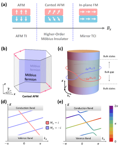
Figure 1: (a) Applying an in-plane field $B_{x}$ to an AFM TI induces a topological transition to a higher-order Möbius insulator, and eventually to a mirror TCI protected by $M_{x}$. (b) Schematic of a higher-order Möbius insulator in a hexagonal geometry. The red arrows represent chiral hinge modes. (c) Schematic of surface Möbius fermions along the glide-invariant line (GIL) labeled with a ${\cal G}_{x}$ eigenvalue of $\pm ie^{ik_{z}/2}$. Along GIL, the Möbius fermions can be disconnected from other bands. We schematically show how the surface state of a mirror TCI in (d) evolves into a Möbius fermion in (e), when the mirror symmetry is broken to ${\cal G}_{x}$. The color bar in (e) shows the phase of the corresponding ${\cal G}_{x}$ eigenvalue. A gap opens when two surface states with the same color cross.

Introduction - The past decade has witnessed the rapid development of topological crystalline insulators (TCI) as a new class of materials Fu (2011); Hsieh et al. (2012); Mong et al. (2010); Ando and Fu (2015); Liu et al. (2014); Zhang and Liu (2015); Shiozaki et al. (2015); Fang and Fu (2015); Wang et al. (2016); Chang et al. (2017), where crystalline symmetries protect band topology in solids. The bulk topology of a TCI enforces protected in-gap states to emerge only on its symmetry-preserving boundaries. Recently, it was realized that a special class of TCI also features higher-order topology Benalcazar et al. (2017a, b); Schindler et al. (2018a); Langbehn et al. (2017); Khalaf (2018); Khalaf et al. (2018); Zhang et al. (2013), where gapless modes live on $(D-d)$-dimensional boundary of a $D$-dimensional TCI with $1<d\leq D$. Theoretical work on these higher-order topological insulators (HOTI) has mainly focused on topological classifications and model constructions, with only a few realistic candidate materials being proposed Schindler et al. (2018b); Xu et al. (2019a); Yue et al. (2019); Wang et al. (2018); Lee et al. (2019a); Sheng et al. (2019). Experimentally, the only evidence for electronic HOTI was demonstrated in bismuth Schindler et al. (2018b). Therefore, identifying more experimentally accessible HOTI systems is important.

Recently, a major breakthrough for TCI is the discovery of antiferromagnetic (AFM) topological insulators (TI) in MnBi_2nTe_3n+1 family of materials Zhang et al. (2019); Otrokov et al. (2018); Gong et al. (2019); Li et al. (2019a); Vidal et al. (2019a); Hu et al. (2019a); Wu et al. (2019); Li et al. (2019b); Hao et al. (2019); Chen et al. (2019). With intrinsic $A$-type AFM order and an out-of-plane easy axis, the band topology of MnBi_2nTe_3n+1 is protected by an AFM time-reversal symmetry (TRS) $\Theta_{M}$, which combines the TRS operation $\Theta$ and a half-unit-cell translation $T_{[00\frac{1}{2}]}$ along $\hat{z}$ direction. Compounds with $n=1,2,3$ (i.e., MnBi₂Te₄, MnBi₄Te₇, and MnBi₆Te₁₀) are currently under active experimental study Hu et al. (2019a); Wu et al. (2019); Vidal et al. (2019b); Shi et al. (2019); Ding et al. (2019); Tian et al. (2019); Xu et al. (2019b); Hu et al. (2019b); Lee et al. (2019b); Yan et al. (2019a, b). Remarkably, evidence of quantum anomalous Hall effect Deng et al. (2019); Ge et al. (2019) and axion insulator Liu et al. (2019) has recently been reported in few-layer MnBi₂Te₄. Since the magnetic moments of MnBi_2nTe_3n+1 can be easily manipulated by a weak applied magnetic field, it is an interesting open question on the type of band topology that could arise for various field-induced magnetic configurations in MnBi_2nTe_3n+1.

In this Letter, we propose MnBi_2nTe_3n+1 as a highly tunable system to realize a variety of HOTI phases. In particular, we show that applying an in-plane magnetic field cants the AFM ordering and leads to the first material platform for a higher-order Möbius insulator with a Möbius twist in its topological surface state, as schematically shown in Fig. 1. Furthermore, opposite surfaces hosting Möbius states are connected by 1d chiral hinge modes, manifesting the higher-order nature. For general magnetic configurations, two distinct classes of inversion-protected HOTIs are expected in MnBi_2nTe_3n+1. These two HOTI phases share the same bulk topological index but differ in their hinge mode configurations. Rotating the magnetic field can drive transition between these two phases, and therefore, can lead to a topological magnetic switching of $G_{zz}$, the two-terminal conductance along $\hat{z}$ direction. We also discuss experimental consequences and application of our theory to other proposed axion insulators.

Model Hamiltonian - We start by defining an effective Hamiltonian for MnBi_2nTe_3n+1 that captures its essential symmetry and topological features. In the absence of magnetism, the point group of MnBi_2nTe_3n+1 is $D_{3d}$ foo , which can be generated by (i) a three-fold rotation $C_{3z}$ around $z$-axis, (ii) a two-fold rotation $C_{2x}$ around $x$-axis, and (iii) the spatial inversion ${\cal I}$. $D_{3d}$ also contains three in-plane mirror operations including $M_{x}$. Following earlier first-principles calculations Zhang et al. (2019); Vidal et al. (2019b), we consider the basis functions $|\uparrow(\downarrow),\pm\rangle$ with $\pm$ parity eigenvalues. This defines a four-band ${\bf k}\cdot{\bf p}$ Hamiltonian $H_{0}({\bf k})$ around $\Gamma$ point, which resembles that for Bi₂Se₃ Liu et al. (2010) and describes a 3d massive Dirac fermion. In particular, $H_{0}({\bf k})=e({\bf k})\mathbb{I}_{4}+\sum_{i=1}^{5}d_{i}({\bf k})\Gamma_{i}$, where $\mathbb{I}_{4}$ is the identity matrix, $\Gamma_{i}=s_{i}\otimes\sigma_{1}$ for $i=1,2,3$, $\Gamma_{4}=s_{0}\otimes\sigma_{2}$, and $\Gamma_{5}=s_{0}\otimes\sigma_{3}$. $s_{i}$ and $\sigma_{i}$ are the Pauli matrices for the spin and orbital degrees of freedom, respectively. The point group symmetry constrains the explicit forms of $d_{i}({\bf k})$ to be $d_{1}=vk_{x},\ d_{2}=vk_{y},\ d_{3}=v_{z}k_{z},\ d_{4}=w(k_{+}^{3}+k_{-}^{3}),\ d_{5}=M_{0}+M_{1}k_{z}^{2}+M_{2}(k_{x}^{2}+k_{y}^{2})$, and $e({\bf k})=C_{0}+C_{1}k_{z}^{2}+C_{2}(k_{x}^{2}+k_{y}^{2})$. Physically, $v$ and $v_{z}$ denote the in-plane and out-of-plane Fermi velocities, while $w$ controls the hexagonal warping effect and reduces the full rotation symmetry down to $C_{3z}$. For our purpose, we regularize our model on a 3d hexagonal lattice as shown in Fig. 2 (a). The full expression for the lattice model is given in the Supplemental Material (SM) sup .

The pristine MnBi_2nTe_3n+1 compounds usually develop A-type AFM ordering along (001) direction, as shown in Fig. 2 (a), where we introduce a sublayer index $i=A,B$ to describe the AFM-induced unit cell doubling. We characterize the magnetization in sublayer $i$ by ${\bf M}_{i}=(\cos\phi_{i}\sin\theta_{i},\sin\phi_{i}\sin\theta_{i},\cos\theta_{i})$ with angles $\phi_{i}$ and $\theta_{i}$. In particular, the exchange coupling term is

$$H_{\text{ex}}=\begin{pmatrix}{\bf M}_{A}\cdot\vec{s}\otimes\sigma_{0}&0\\ 0&{\bf M}_{B}\cdot\vec{s}\otimes\sigma_{0}\\ \end{pmatrix}.$$ (1)

The AFM ordering is described by $(\theta_{A},\theta_{B})=(0,\pi)$. With a set of band parameters that captures the bulk band inversion at $\Gamma$ sup , we calculate the energy spectrum for the (010) surface of the AFM phase in a semi-infinite geometry using iterative Green function method. As shown in Fig. 2 (b), the system hosts a single gapless Dirac cone at $\bar{\Gamma}$, the origin of surface Brillouin zone (BZ). The gapless Dirac surface state here is protected by the AFM TRS $\Theta_{M}$ and generally shows up for any surface that is compatible with $\Theta_{M}$ symmetry Mong et al. (2010). On the other hand, a finite surface energy gap is expected on the (001) surface. The AFM TI phase serves as the starting point for our discussion on higher-order topology.

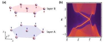
Figure 2: (a) Lattice structure of our tight-binding model. (b) Surface spectrum for (010) surface of the AFM phase.

Higher-Order Möbius Insulator - In the presence of an external in-plane magnetic field ${\bf B}$, the AFM cants along the field direction [see Fig. 1 (a) and discussions in the SM sup ] and generally breaks all symmetries except for the spatial inversion ${\cal I}$. The loss of $\Theta_{M}$ generally leads to a magnetic surface gap for every surface and trivializes the $\Theta_{M}$-protected topology. However, this enables the possibility of higher-order topology emerging in this system.

When ${\bf B}$ is along $\hat{x}$ and hence perpendicular to the $M_{x}$ mirror plane, the canted AFM ordering respects a non-symmorphic glide mirror symmetry ${\cal G}_{x}$ that combines mirror reflection $M_{x}$ and the half-unit-cell translation $T_{[00\frac{1}{2}]}$ along $\hat{z}$, as shown in Fig. 3 (a). Along the glide-invariant line (GIL) of the nonsymmorphic 010 surface BZ (e.g. $k_{x}=0,\pi$), the surface states are labeled by their glide eigenvalues $g_{x}=\pm ie^{ik_{z}/2}$. Whenever surface states with distinct $g_{x}$ cross, a “locally” robust surface Dirac point is formed. Nevertheless, only an odd number of surface Dirac points is topologically robust for this system, featuring $\mathbb{Z}_{2}$ band topology Fang and Fu (2015); Shiozaki et al. (2015). This motivates us to calculate the (010) surface spectrum for our canted AFM system. As shown in Fig. 3 (b), a single surface Dirac point is clearly revealed along GIL, which proves the topological nature of the canted AFM phase.

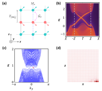
Figure 3: (a) When magnetic moments in the canted AFM cant towards $\hat{x}$ direction, the system has a glide mirror symmetry ${\cal G}_{x}$, which interchanges the green and red magnetic moments. (b) The surface spectrum on (010) surface for the canted AFM phase with $\theta_{A}=\pi-\theta_{B}=0.3\pi$ and $\phi_{A}=\phi_{B}=0$. The glide-invariant line is sanwiched between two white dashed lines, where the Möbius fermion is well-defined. (c) The corresponding in-gap chiral hinge modes in a prism geometry periodic in $\tilde{y}$ direction. (d) The real-space distribution in the $x$-$z$ plane for the chiral modes marked by the red dot in (c).

While the crystal momentum is $2\pi$ periodic along GIL, the glide eigenvalue $g_{x}$ follows a periodicity of $4\pi$ due to the half-unit-cell translation. Therefore, the surface state manifold along GIL manifests itself as a Möbius twist for $g_{x}$ Shiozaki et al. (2015); Wang et al. (2016); Chang et al. (2017); Wieder et al. (2018), as schematically plotted in Fig. 1 (c). We thus dub this surface state as 2d “Möbius fermions”. Distinct from conventional surface states of topological insulators, the Möbius fermions can be disconnected from other surface or bulk bands along GIL, but are connected to higher-energy bands away from GIL for being unremovable. In our canted AFM phase, Möbius fermions only live on the (010) surfaces [i.e., the purple surfaces in Fig. 1 (b)] where glide symmetry is preserved, while surface gaps show up on all other surfaces. The topological characterization of the Möbius fermions using Wilson loop method is discussed in the SM sup .

Remarkably, there exist hinge-localized 1d chiral modes that connect the opposite (010) surfaces with Möbius fermions, as shown in Fig. 1 (b). Indeed, while the glide symmetry ${\cal G}_{x}$ allows for a $\mathbb{Z}_{2}$ invariant $\nu_{g}$ to characterize the Möbius fermions, a $\mathbb{Z}_{4}$ symmetry indicator $\kappa$ for the inversion symmetry ${\cal I}$ can be simultaneously defined as Turner et al. (2012); Ono and Watanabe (2018)

$$\kappa\equiv\sum_{k_{i}}\frac{(n_{+}-n_{-})}{2}\ \ (\text{mod }4).$$ (2)

Here $n_{\pm}$ counts the number of occupied bands with $\pm$ parity eigenvalues and the summation is over all inversion-symmetric crystal momenta. Physically, an odd $\kappa$ implies a Weyl semimetal. When a system is known to be gapped, the $\kappa=2$ phase is an axion insulator with higher-order topology Wieder and Bernevig (2018). Crucially, symmetry argument imposes a relation between $\nu_{g}$ and $\kappa$ as Kim et al. (2019)

$$\nu_{g}\equiv\frac{\kappa}{2}\ \ \text{mod }2.$$ (3)

As a result, when Möbius fermions show up ($\nu_{g}=1$), the chiral hinge mode is required to appear because of $\kappa=2$, and vice versa.

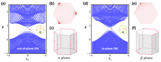
Figure 4: (a) The hinge mode spectrum of the HOTI $\alpha$ phase with $\theta_{A}=\theta_{B}=0$. (b) The spatial profile of the left-moving hinge modes indicated by the red dot in (a), which confirms the schematic plot in (c). (d)-(f) Corresponding plots for the HOTI $\beta$ phase. $\phi_{A}=\phi_{B}=\frac{\pi}{6}$ and $\theta_{A}=\theta_{B}=\frac{\pi}{2}$ for calculations done in (d) and (e).

A simple topological index analysis in the SM sup implies $\kappa=2$ in our model if the transition from AFM to canted AFM does NOT close the bulk gap. Numerically, we consider a prism geometry periodic along $\tilde{y}$ with a finite cross section in its $x$-$z$ plane ($20\times 21$ lattice sites). Note that $\tilde{y}$ differs from the Cartesian-coordinate $\hat{y}$ axis by a $\pi/6$ rotation around $\hat{z}$. Fig. 3 (c) plots the energy spectrum in this prism geometry, showing 1d chiral modes that traverse the surface gaps. In Fig. 3 (d), we depict the spatial profile of the left-moving mode in the $x$-$z$ cross section and find it localized at the bottom right corner, which verifies the hinge-mode picture. The existence of Möbius fermions on (010) surface and 1d chiral hinge modes along $\tilde{y}$ direction together establishes our canted AFM phase as a “higher-order Möbius insulator”.

By gradually increasing the in-plane ${\bf B}$ field, the canted AFM phase eventually evolves to an in-plane FM phase, which promotes the glide symmetry ${\cal G}_{x}$ to a mirror symmetry $M_{x}$. As shown in Fig. 1 (a), the higher-order Möbius phase thus evolves to a mirror-protected TCI Hsieh et al. (2012); Vidal et al. (2019b) with no hinge physics. The transition from a Möbius fermion to a mirror-protected topological surface state is schematically shown in Figs. 1(d) and 1(e).

Inversion-Protected Higher-Order Topology - When ${\bf B}$ deviates from $\hat{x}$, various new magnetic configurations can be induced that generally break the glide symmetry ${\cal G}_{x}$ and thus spoil the Möbius physics, as well as the mirror TCI physics. Despite energy gaps on all surfaces because of lack of symmetries sup , the inversion indicator $\kappa=2$ remains well-defined as long as the bulk gap survives, which characterizes our system as a robust inversion-symmetric higher-order TI Khalaf (2018); Khalaf et al. (2018) with chiral hinge mode. In particular, there exist two classes of inversion-symmetric HOTI phases in MnBi_2nTe_3n+1, which we discuss next.

When MnBi_2nTe_3n+1 is ferromagnetic along $\hat{z}$, it realizes a HOTI that preserves three-fold rotation symmetry $C_{3z}$. When placed on a hexagonal geometry, the hinge mode configuration compatible with both inversion ${\cal I}$ and $C_{3z}$ is shown in Fig. 4 (c), which consists of three spatially separated chiral hinge modes along $+\hat{z}$ along with their inversion partners on the opposite hinges. We call this phase the HOTI $\alpha$ phase to distinguish it from the $\beta$ phase defined later. Numerically, we calculate the energy spectrum of this out-of-plane ferromagnet in the hexagonal prism geometry with in-plane open boundary conditions and with periodicity in $\hat{z}$ direction. As shown in Fig. 4 (a), we find three pairs of 1d modes that traverse the surface gap, which are further confirmed as chiral hinge modes by their spatial profiles plotted in Fig. 4 (b). These results together confirm the schematic in Fig. 4 (c).

In contrast, the HOTI $\beta$ phase is defined by the chiral hinge mode trajectory shown in Fig. 4 (f), which explicitly breaks $C_{3z}$ and has only one pair of chiral hinge modes along $\hat{z}$. The $\beta$ phase can be induced by applying a magnetic field off the high-symmetry directions, which holds for generic magnetic structures in MnBi_2nTe_3n+1. An example of $\beta$ phase with FM ordering is numerically confirmed in Fig. 4 (d) and (e). In the SM sup , we provide a second example of $\beta$ phase with canted AFM ordering. We emphasize that $\alpha$ and $\beta$ phases share the same bulk index $\kappa=2$ and are hence topologically equivalent. Although phenomenologically distinct, an $\alpha$ phase can be transformed into a $\beta$ phase by symmetrically attaching 2d layers of Chern insulator to the side surfaces. In other words, $\alpha$ phase can be connected to $\beta$ phase by only closing its surface gaps, which can be achieved by manipulating its bulk magnetic ordering via ${\bf B}$ field sup .

Experiment Signatures - For a finite-slab geometry, the chiral hinge modes in both $\alpha$ and $\beta$ phases enable in-plane quantized anomalous Hall conductance $\sigma_{xy}=e^{2}/h$. Notably, this conductance quantization to $e^{2}/h$ persists when the slab thickness grows, which signals 3d higher-order topology. In addition, we suggest using scanning tunneling microscopy to map out the in-gap local density of states (LDOS) on the top surface. As shown in Fig. 5 (a), we predict that for a HOTI $\alpha$ phase, the LDOS on the top surface only peaks at some specific hinges or step edges. As a comparison, we also plot the in-gap LDOS peak of a 2d Chern insulator, which generally appears on all edges [Fig. 5 (b)]. This special LDOS pattern of the chiral hinge modes provides another direct experimental evidence for higher-order topology.

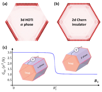
Figure 5: In-gap LDOS for (a) the top surface of a HOTI $\alpha$ phase and (b) a 2d Chern insulator. (c) The transition from HOTI $\alpha$ phase to $\beta$ phase is accompanied by a quantized jump in $G_{zz}$, which realizes a topological magnetic switch.

Meanwhile, $\alpha$ and $\beta$ phases behave distinctly in their out-of-plane transport measurements. In Fig. 5 (c), we propose measuring the two-terminal conductance $G_{zz}=I_{z}/V_{z}$ by driving a $\hat{z}$-directional current $I_{z}$ and measuring the voltage drop $V_{z}$ between top and bottom surfaces. Although quantized signals are expected for both phases, the $\alpha$ phase has $G_{zz}=3e^{2}/h$ while the $\beta$ phase has $G_{zz}=e^{2}/h$. Since an in-plane magnetic field ${\bf B}_{\parallel}$ generally drives the transition between these phases, this device realizes a “topological magnetic switch”, where the ${\bf B}_{\parallel}$ controls a quantized jump of $G_{zz}$ by a factor of 3 [Fig. 5 (c)]. Remarkably, the threshold for $B_{\parallel}$ to trigger this switching could be as low as $0.2$ T Hu et al. (2019a); Vidal et al. (2019b), which holds promise for practical topological electronics.

Conclusion - We have proposed MnBi_2nTe_3n+1 as a possible material class for realizing higher-order Möbius physics and various inversion-symmetric higher-order topological phases. For MnBi₂Te₄, MnBi₄Te₇, and MnBi₆Te₁₀, A-type AFM physics have been reported at zero field and signatures of canted AFM have been observed with an in-plane magnetic field Gong et al. (2019); Hu et al. (2019a); Wu et al. (2019); Vidal et al. (2019b); Shi et al. (2019); Tian et al. (2019). Based on our topological index analysis, we expect those canted AFM systems to be exactly our proposed higher-order Möbius insulators, when the magnetic field is carefully aligned to preserve the glide symmetry.

For both MnBi₄Te₇ and MnBi₆Te₁₀, an out-of-plane FM phase is observed at a small ($\sim$0.2 T) Hu et al. (2019a); Wu et al. (2019); Vidal et al. (2019b) or even vanishing field Shi et al. (2019); Tian et al. (2019). Recent first-principles calculations suggest a non-trivial symmetry indicator $\kappa=2$ for the FM phases in both materials Vidal et al. (2019b); Tian et al. (2019), which supports our prediction of the HOTI $\alpha$ phase in these FM systems. Moreover, the HOTI $\beta$ phase and the topological magnetic switch effect can be feasibly achieved by simply rotating the magnetic field.

Finally, we emphasize that our theory provides a microscopic mechanism for higher-order Möbius insulators in magnetic topological materials. For example, the higher-order Möbius physics can also be realized on the (010) surface of the afmc phase in the axion insulator candidate EuIn₂As₂ Xu et al. (2019a) when an external in-plane field cants the magnetic moments. Similar physics can also be expected for other candidate axion insulators, such as EuSn₂As₂ Li et al. (2019b) and EuSn₂P₂ Gui et al. (2019). With the recent rapid developments in this field, we believe that our proposed Möbius and higher-order topological phases should soon be experimentally realizable.

Acknowledgment - We thank Yang-Zhi Chou, Sheng-Jie Huang, Jiabin Yu, and Zhida Song for helpful discussions. This work is supported by the Laboratory for Physical Sciences and Microsoft. R.X.Z acknowledges a JQI postdoctoral fellowship.

.1 Supplemental Material for “Möbius Insulator and Higher-Order Topology in MnBi_2nTe_3n+1”

I Appendix A: Lattice Model

We start by defining our effective lattice model. The continuum model in the main text is regularized on a 3d hexagonal lattice, which is defined by the lattice constants ${\bf a}_{1}=(1,0,0)^{T},\ {\bf a}_{2}=\frac{1}{2}(1,\sqrt{3},0)^{T},\ {\bf a}_{3}=(0,0,1)^{T}$. For our purpose, we further define the crystal momenta $(k_{1},k_{2},k_{z})$ as

$$k_{1}=k_{x},\ k_{2}=\frac{1}{2}(k_{x}+\sqrt{3}k_{y}).$$ (4)

The full lattice model is given by

$$H=H_{\text{lat}}+H_{ex}$$ (5)

where the exchange-coupling term $H_{ex}$ is defined in Eq. [1] in the main text. The normal part

$$H_{\text{lat}}=\begin{pmatrix}h&h_{AB}\\ h_{AB}^{\dagger}&h\\ \end{pmatrix},$$ (6)

Here the intra-layer Hamiltonian is

$$h = (\tilde{C}-\frac{4}{3}C_{2}[\cos k_{1}+\cos k_{2}+\cos(k_{1}-k_{2})])\mathbb{I}_{4}+\frac{2v}{3}(\sin k_{1}+\frac{1}{2}[\sin(k_{1}-k_{2})+\sin k_{2}])\Gamma_{1}$$ (7)

$$+(\frac{v}{\sqrt{3}}[\sin k_{2}-\sin(k_{1}-k_{2})])\Gamma_{2}+w[-\sin k_{1}+\sin k_{2}+\sin(k_{1}-k_{2})]\Gamma_{4}$$

$$+(\tilde{M}-\frac{4}{3}M_{2}[\cos k_{1}+\cos k_{2}+\cos(k_{1}-k_{2})])\Gamma_{5},$$

where $\tilde{C}=C_{0}+2C_{1}+4C_{2}$ and $\tilde{M}=M_{0}+2M_{1}+4M_{2}$. The hopping between layer A and layer B is described by

$$h_{AB}=-2C_{1}\cos\frac{k_{z}}{2}\mathbb{I}_{4}+2v_{z}\sin\frac{k_{z}}{2}\Gamma_{3}-2M_{1}\cos\frac{k_{z}}{2}\Gamma_{5}.$$ (8)

By expanding $H_{\text{lat}}$ around $\Gamma$ point, it reproduces the continuum Hamiltonian in the main text.

We have used $M_{0}=-2,M_{1}=1,M_{2}=1,C_{0}=0,C_{1}=0.3,C_{2}=0.4,v_{z}=1,v=0.5,m=0.4,w=1.5$ as our choice of parameters throughout the work.

II Appendix B: Equivalent Relations Among Symmetry Indicators

In this section, we discuss the equivalent relations among the inversion symmetry indicators for various topological phases that appear in our system. In a time-reversal-symmetric system with inversion symmetry, we can define a $\mathbb{Z}_{4}$ symmetry indicator

$$\kappa_{\Theta}=\frac{1}{4}\sum_{k_{i}}(n_{+}-n_{-})\ \ (\text{mod }4).$$ (9)

Here $n_{+}$ and $n_{-}$ are the numbers of occupied bands with $+$ and $-$ parity eigenvalues, respectively, which are summed over eight time-reversal-invariant momenta $k_{i}$ in a 3d BZ. While an odd (even) $\kappa$ implies existence (absence) of a strong TI phase, $\kappa=2$ characterizes a HOTI phase with 1d helical hinge states.

When AFM is introduced and the TRS is broken to an AFM TRS, the band topology is characterized by a similar $\mathbb{Z}_{2}$ inversion indicator $\xi\in\mathbb{Z}_{2}$ with

$$\xi=\frac{1}{4}\sum_{k_{i}}(n_{+}-n_{-})\ \ (\text{mod }2).$$ (10)

Clearly, by definition,

$$\xi=\kappa_{\Theta}\ \ (\text{mod }2).$$ (11)

This leads to the following statement:

• By adiabatically breaking TRS to an AFM TRS while preserving inversion, a 3d strong TI with $\kappa_{\Theta}=1,3$ is connected to an AFM TI with $\xi=1$.

For the magnetic higher-order topological physics discussed in our system, it is indicated by a new $\mathbb{Z}_{4}$ indicator

$$\kappa=\frac{1}{2}\sum_{k_{i}}(n_{+}-n_{-})\ \ (\text{mod }4),$$ (12)

which is Eq. [2] in the main text. To see the connection between $\xi$ and $\kappa$, we note that the parity eigenvalues obey

$$\sum_{k_{i}}(n_{+}-n_{-})=4(2l+\xi),$$ (13)

following Eq. 10, where $l\in\mathbb{Z}$ is an integer. Therefore,

$$\kappa = 4m+2\xi\ \ (\text{mod }4)$$ (14)

$$\equiv 2\xi\ \ (\text{mod }4).$$

As a result, we arrive at an important conclusion:

• By adiabatically breaking $\Theta_{M}$ while preserving inversion, a 3d AFM TI with $\xi=1$ is connected to an axion insulator with $\kappa=2$ and higher-order topology.

Here we have included the BZ folding effect of AFM in the definitions of $\kappa,\kappa_{\Theta}$, and $\xi$.

III Appendix C: Wilson Loop Characterization for Möbius Fermion

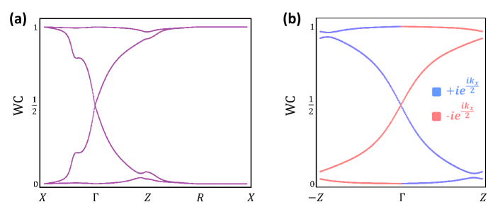
Figure 6: (a) Gapless WC flows along the high symmetry lines reveals nontrivial surface state on the (010) surface. (b) The Möbius pattern of WC flows along the glide-invariant line. Different colors denote different glide-mirror sectors.

In this section, we discuss the nontrivial Wilson loop spectrum that characterizes the topological nature of the higher-order Möbius insulator. The Wilson loop along a closed path $L$ in the momentum space is defined as

$${\cal W}_{L}=\text{exp}[i\oint_{L}{\bf A}d{\bf k}],$$ (15)

where the non-Abelian Berry connection

$${\bf A}_{mn}({\bf k})=i\langle u_{m}({\bf k})|\nabla_{\bf k}|u_{n}({\bf k})\rangle.$$ (16)

For given $k_{x}$ and $k_{z}$, the phases of the eigenvalues for the Wilson loop

$${\cal W}_{y}(k_{x},k_{z})=\text{exp}[i\int_{0}^{2\pi}dk_{y}{\bf A}(k_{y})]$$ (17)

are the Wannier centers (WC), or equivalently the 1d electronic polarization along $\hat{y}$. Physically, the evolution of WCs in the 2d BZ spanned by $k_{x}$ and $k_{z}$ describe the charge pumping process on the $(010)$ surface.

In Fig. 6 (a), we calculate the evolution of WC flows along the high symmetry lines that are perpendicular to the $k_{y}$ axis. Crucially, the two WC flows show a nontrivial gapless winding pattern along the high symmetry lines, featuring a topological gapless surface state on the $(010)$ surface. This WC pattern is similar to that of the hourglass fermion in Ref. Wang et al. (2016).

As shown in Fig. 6 (b), we plot the WC flows along the glide-invariant line (GIL) from $-Z$ to $Z$ via $\Gamma$. Since the Hamiltonian is block-diagonal along GIL, the WC flow for each glide-mirror sector can be individually plotted. In particular, we find that the WC flow along GIL also has a Möbius nature, manifesting the bulk-boundary correspondence.

IV Appendix D: Effective Surface Theory

In this section, we establish an effective surface theory to understand the formation of chiral hinge modes and the surface topological transition of HOTI $\alpha$ and $\beta$ phases. To start with, consider a Hamiltonian $H({\bf k})$ for HOTI $\alpha$ phase, which describes a 3d topological insulator with out-of-plane FM.

$$H({\bf k})=\begin{pmatrix}e({\bf k})+M({\bf k})+g_{z}&v_{z}k_{z}&0&v(k_{x}-ik_{y})\\ v_{z}k_{z}&e({\bf k})-M({\bf k})+g_{z}&v(k_{x}-ik_{y})&0\\ 0&v(k_{x}+ik_{y})&e({\bf k})+M({\bf k})-g_{z}&-v_{z}k_{z}\\ v(k_{x}+ik_{y})&0&-v_{z}k_{z}&e({\bf k})-M({\bf k})-g_{z}\\ \end{pmatrix},$$ (18)

with $M({\bf k})=M_{0}+M_{1}k_{z}^{2}+M_{2}(k_{x}^{2}+k_{y}^{2})$ and $C({\bf k})=C_{2}k_{y}^{2}$. Here we have ignored the $k_{x}^{2}$ and $k_{z}^{2}$ terms in $C{\bf k}$ for simplicity. $g_{z}$ chracterizes the FM exchange coupling parallel to $\hat{z}$. For our purpose, we focus on the (010) surface theory which will be solved by replacing $k_{y}$ with $-i\partial_{y}$. The Hamiltonian can be then separated into two parts,

$$H_{\perp}(-i\partial_{y})=$$

$$\begin{pmatrix}-(M_{2}+C_{2})\partial_{y}^{2}+(M_{0}+g_{z})&0&0&-v\partial_{y}\\ 0&(M_{2}-C_{2})\partial_{y}^{2}-(M_{0}-g_{z})&-v\partial_{y}&0\\ 0&v\partial_{y}&-(M_{2}+C_{2})\partial_{y}^{2}+(M_{0}-g_{z})&0\\ v\partial_{y}&0&0&(M_{2}-C_{2})\partial_{y}^{2}-(M_{0}+g_{z})\\ \end{pmatrix},$$

and

$$H_{\parallel}(k_{x},k_{z})=\begin{pmatrix}M_{1}k_{z}^{2}+M_{2}k_{x}^{2}&v_{z}k_{z}&0&vk_{x}\\ v_{z}k_{z}&-(M_{1}k_{z}^{2}+M_{2}k_{x}^{2})&vk_{x}&0\\ 0&vk_{x}&M_{1}k_{z}^{2}+M_{2}k_{x}^{2}&-v_{z}k_{z}\\ vk_{x}&0&-v_{z}k_{z}&-(M_{1}k_{z}^{2}+M_{2}k_{x}^{2})\\ \end{pmatrix},$$ (20)

In particular, $H_{\perp}$ consists of two $2$ by $2$ blocks,

$$h_{14}=\begin{pmatrix}-(M_{2}+C_{2})\partial_{y}^{2}+(M_{0}+g_{z})&-v\partial_{y}\\ v\partial_{y}&(M_{2}-C_{2})\partial_{y}^{2}-(M_{0}+g_{z})\\ \end{pmatrix},$$ (21)

and

$$h_{23}=\begin{pmatrix}(M_{2}-C_{2})\partial_{y}^{2}-(M_{0}-g_{z})&-v\partial_{y}\\ v\partial_{y}&-(M_{2}+C_{2})\partial_{y}^{2}+(M_{0}-g_{z})\\ \end{pmatrix}.$$ (22)

IV.1 Surface State Solution

We note that $h_{23}$ is exactly $h_{14}$ if we flip the sign of $M_{0}$ and $M_{2}$. Thus, we only need to solve for the surface state of $h_{14}$. Let us define $m_{g}=M_{0}+g_{z}$ and consider a trial surface state solution at an energy $E$,

$$\psi=\begin{pmatrix}A\\ B\\ \end{pmatrix}e^{-\lambda y},\ \ h_{14}\psi=E\psi.$$ (23)

This leads to

$$\begin{pmatrix}m_{g}-(M_{2}+C_{2})\lambda^{2}-E&v\lambda\\ -v\lambda&-m_{g}+(M_{2}-C_{2})\lambda^{2}-E\\ \end{pmatrix}\begin{pmatrix}A\\ B\\ \end{pmatrix}=0.$$ (24)

Therefore, we have

$$\psi_{E}=\begin{pmatrix}-m_{g}+(M_{2}-C_{2})\lambda^{2}-E\\ v\lambda\\ \end{pmatrix}e^{-\lambda y}$$ (25)

For a given energy $E$, we notice that Eq. 24 implies the existence of two decay soluations $\lambda_{1,2}$. Therefore, $\psi_{E}$ should be modified to

$$\psi_{E}={\cal N}_{1}\begin{pmatrix}-m_{g}+(M_{2}-C_{2})\lambda_{1}^{2}-E\\ v\lambda_{1}\\ \end{pmatrix}e^{-\lambda_{1}y}+{\cal N}_{2}\begin{pmatrix}-m_{g}+(M_{2}-C_{2})\lambda_{2}^{2}-E\\ v\lambda_{2}\\ \end{pmatrix}e^{-\lambda_{2}y}$$ (26)

where ${\cal N}_{1,2}$ are the normalization factors. The boundary condition at $y=0$ enforces the vanishing of the surface state wavefunction and we find that

$$\begin{pmatrix}-m_{g}+(M_{2}-C_{2})\lambda_{1}^{2}-E&-m_{g}+(M_{2}-C_{2})\lambda_{2}^{2}-E\\ v\lambda_{1}&v\lambda_{2}\\ \end{pmatrix}\begin{pmatrix}{\cal N}_{1}\\ {\cal N}_{2}\end{pmatrix}=0$$ (27)

This immediately leads to

$$\lambda_{1}\lambda_{2}=-\frac{E+m_{g}}{M_{2}-C_{2}}.$$ (28)

On the other hand, following Eq. 24, we have

$$(C_{2}^{2}-M_{2}^{2})\lambda^{4}+(v^{2}+2M_{2}m_{g}+2C_{2}E)\lambda^{2}+(E^{2}-m_{g}^{2})=0$$ (29)

and consequently

$$\lambda_{1}\lambda_{2}=\frac{E^{2}-m_{g}^{2}}{C_{2}^{2}-M_{2}^{2}}.$$ (30)

Together, since $\lambda_{1}\lambda_{2}\neq 0$, we have

$$E_{14}=-\frac{(M_{0}+g_{z})C_{1}}{M_{2}}.$$ (31)

Plug it into Eq. 29 and complete the square, we arrive at

$$(\lambda^{2}-\frac{m_{g}}{M_{2}})^{2}=-\frac{(v\lambda)^{2}}{C_{1}^{2}-M_{2}^{2}}.$$ (32)

and eventually we find that the spinor part of $\psi_{E}$ is

$$\xi_{14}=\begin{pmatrix}\sqrt{\frac{M_{2}-C_{1}}{M_{2}+C_{1}}}\\ 1\\ \end{pmatrix}$$ (33)

Similarly, one can obtain

$$E_{23}=\frac{(-M_{0}+g_{z})C_{1}}{M_{2}},\ \ \xi_{23}=\begin{pmatrix}\sqrt{\frac{M_{2}+C_{1}}{M_{2}-C_{1}}}\\ -1\\ \end{pmatrix}$$ (34)

IV.2 Surface Hamiltonian and the Gap

With the surface states in Eq. 33 and Eq. 34, the projection of $H_{\parallel}$ is straightforward. Up to ${\cal O}(k)$ and ignoring the identity term, we have

$$H_{ss}=\tilde{v}k_{x}\sigma_{z}+\tilde{v}_{z}k_{z}\sigma_{x}-\frac{g_{z}C_{1}}{M_{2}}\sigma_{z}.$$ (35)

Therefore, with out-of-plane FM, the surface Dirac point of (010) surface only gets shifted from the origin of surface BZ to $k_{x}=\frac{g_{z}C_{1}}{\tilde{v}M_{2}}$. The surface gap opens up only when we include the hexagonal warping effect. We find that $H_{ss}$ is modified to

$$H_{ss}=\tilde{v}k_{x}\sigma_{z}+\tilde{v}_{z}k_{z}\sigma_{x}-\frac{g_{z}C_{1}}{M_{2}}\sigma_{z}+\tilde{w}k_{x}^{3}\sigma_{y}.$$ (36)

Therefore, the surface gap of (010) surface is a combined efect of out-of-plane FM $g_{z}$, the particle-hole breaking $C_{1}$, and the hexagonal warping $w$. Since the momentum part of the hexagonal warping term is invariant under $C_{3z}$ but odd under inversion, it is expected that the hinge between neighboring surfaces on the hexagonal prism [in Fig. 4(c) of the main text] forms a mass domain wall for 2d Dirac fermions, which explains the existence of chiral hinge modes.

IV.3 Surface Transition between HOTI $\alpha$ and $\beta$ Phases

When the FM moment is rotated by the magnetic field and has an in-plane component, the surface topological transition between $\alpha$ and $\beta$ phases can be induced. In the bulk Hamiltonian, we consider a y-directional Zeeman term $g_{y}s_{y}\otimes\sigma_{0}$. Upon projection, we arrive at

$$H_{ss}=\tilde{v}k_{x}\sigma_{z}+\tilde{v}_{z}k_{z}\sigma_{x}-\frac{gC_{1}}{M_{2}}\sigma_{z}+(\tilde{w}k_{x}^{3}-\tilde{g}_{y})\sigma_{y}.$$ (37)

The transition happens when the surface gap closes. This is only possible when

$$\tilde{g}_{y}=\tilde{w}k_{x}^{3}=\frac{C_{1}^{3}\tilde{w}}{\tilde{v}^{3}M_{2}^{3}}g_{z}^{3}.$$ (38)

V Appendix E: HOTI $\beta$ Phase with Canted AFM

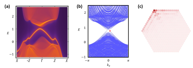
Figure 7: (a) The (010) surface spectrum calculated using iterative Green function method. (b) The energy spectrum in a prism geometry as a function of $k_{z}$. (c) The wavefunction distribution of the left-moving mode shown by the red dot in (b).

In this section, we provide an example of HOTI $\beta$ phase with canted AFM ordering. The canted AFM we consider is characterized by $\phi_{A}=\phi_{B}=\pi/6$, $\theta_{A}=0.3\pi$ and $\theta_{B}=0.7\pi$, which explicitly breaks both $\Theta_{M}$, $C_{3z}$, $M_{x}$ and the glide mirror ${\cal G}_{x}$. The spatial inversion ${\cal I}$, however, remains preserved.

The surface dispersion on the (010) surface is calculated and shown in Fig. 7 (a). Just as we expect, the surface spectrum displays a finite energy gap due to symmetry breaking. We then calculate the energy spectrum in the prism geometry with the periodic boundary condition applied along $z$ direction. Inside the surface gap, there exists a pair of spatially-separated counterpropagating hinge modes that are locally chiral. For example, the spatial profile of the left-moving chiral channel is plotted in Fig. 7 (c).

The results in Fig. 7 unambiguously establish this phase as a HOTI $\beta$ phase defined in the main text.

VI Appendix F: Macrospin Approximation for Field-Induced Canted AFM

In the AFM phase of MnBi_2nTe_3n+1, the easy axis of the magnetic moment is along the out-of-plane $\hat{z}$ direction. When an external magnetic field ${\bf B}$ is applied perpendicular to this easy axis, the magnetic moments cant towards the field direction. This canting effect can be described by the Stoner-Wohlfarth model Baltz et al. (2018). In the macrospin approximation, the magnetic energy per magnetic unit cell is given by

$$\mathcal{E}=2J_{AF}{\bf M}_{A}\cdot{\bf M}_{B}-K(M_{A,z}^{2}+M_{B,z}^{2})-g({\bf M}_{A}+{\bf M}_{B})\cdot{\bf B},$$ (39)

where ${\bf M}_{A,B}$ are unit vectors representing the direction of magnetic moments, $J_{AF}>0$ is the antiferromagnetic exchange coupling, $K>0$ is the uniaxial anisotropy, and $g$ is the effective Zeeman coupling.

When ${\bf B}$ field is along in-plane $\hat{x}$ direction, ${\bf M}_{A}$ and ${\bf M}_{B}$ build up equal $\hat{x}$ component. The energy density $\mathcal{E}$ can be minimized by the canted AFM ansatz ${\bf M}_{A}=(n_{x},0,\sqrt{1-n_{x}^{2}})$ and ${\bf M}_{B}=(n_{x},0,-\sqrt{1-n_{x}^{2}})$, where $|n_{x}|<1$. In terms of $n_{x}$, $\mathcal{E}$ is given by:

$$\mathcal{E}=2(2J_{AF}+K)n_{x}^{2}-2gn_{x}B_{x}-2(J_{AF}+K).$$ (40)

For a small in-plane ${\bf B}$ field, $\mathcal{E}$ is minimized by

$$n_{x}=\frac{g}{2(2J_{AF}+K)}B_{x}.$$ (41)

Therefore, the in-plane moments grow linearly with the in-plane field before saturating at $B_{x}^{*}=2(2J_{AF}+K)/g$. When $B_{x}$ exceeds $B_{x}^{*}$, the canted AFM phase is transformed to the in-plane ferromagnetic phase, as schematically plotted in Fig. 1(a) of the main text.

References

- Fu (2011) L. Fu, Phys. Rev. Lett. 106, 106802 (2011).
- Hsieh et al. (2012) T. H. Hsieh, H. Lin, J. Liu, W. Duan, A. Bansil, and L. Fu, Nature Communications 3, 982 (2012).
- Mong et al. (2010) R. S. K. Mong, A. M. Essin, and J. E. Moore, Phys. Rev. B 81, 245209 (2010).
- Ando and Fu (2015) Y. Ando and L. Fu, Annual Review of Condensed Matter Physics 6, 361 (2015).
- Liu et al. (2014) C.-X. Liu, R.-X. Zhang, and B. K. VanLeeuwen, Phys. Rev. B 90, 085304 (2014).
- Zhang and Liu (2015) R.-X. Zhang and C.-X. Liu, Phys. Rev. B 91, 115317 (2015).
- Shiozaki et al. (2015) K. Shiozaki, M. Sato, and K. Gomi, Phys. Rev. B 91, 155120 (2015).
- Fang and Fu (2015) C. Fang and L. Fu, Phys. Rev. B 91, 161105 (2015).
- Wang et al. (2016) Z. Wang, A. Alexandradinata, R. J. Cava, and B. A. Bernevig, Nature 532, 189 EP (2016).
- Chang et al. (2017) P.-Y. Chang, O. Erten, and P. Coleman, Nature Physics 13, 794 EP (2017).
- Benalcazar et al. (2017a) W. A. Benalcazar, B. A. Bernevig, and T. L. Hughes, Science 357, 61 (2017a).
- Benalcazar et al. (2017b) W. A. Benalcazar, B. A. Bernevig, and T. L. Hughes, Phys. Rev. B 96, 245115 (2017b).
- Schindler et al. (2018a) F. Schindler, A. M. Cook, M. G. Vergniory, Z. Wang, S. S. P. Parkin, B. A. Bernevig, and T. Neupert, Science Advances 4 (2018a), 10.1126/sciadv.aat0346.
- Langbehn et al. (2017) J. Langbehn, Y. Peng, L. Trifunovic, F. von Oppen, and P. W. Brouwer, Phys. Rev. Lett. 119, 246401 (2017).
- Khalaf (2018) E. Khalaf, Phys. Rev. B 97, 205136 (2018).
- Khalaf et al. (2018) E. Khalaf, H. C. Po, A. Vishwanath, and H. Watanabe, Phys. Rev. X 8, 031070 (2018).
- Zhang et al. (2013) F. Zhang, C. L. Kane, and E. J. Mele, Phys. Rev. Lett. 110, 046404 (2013).
- Schindler et al. (2018b) F. Schindler, Z. Wang, M. G. Vergniory, A. M. Cook, A. Murani, S. Sengupta, A. Y. Kasumov, R. Deblock, S. Jeon, I. Drozdov, H. Bouchiat, S. Guéron, A. Yazdani, B. A. Bernevig, and T. Neupert, Nature Physics 14, 918 (2018b).
- Xu et al. (2019a) Y. Xu, Z. Song, Z. Wang, H. Weng, and X. Dai, Phys. Rev. Lett. 122, 256402 (2019a).
- Yue et al. (2019) C. Yue, Y. Xu, Z. Song, H. Weng, Y.-M. Lu, C. Fang, and X. Dai, Nature Physics 15, 577 (2019).
- Wang et al. (2018) Z. Wang, B. J. Wieder, J. Li, B. Yan, and B. A. Bernevig, arXiv preprint arXiv:1806.11116 (2018).
- Lee et al. (2019a) E. Lee, R. Kim, J. Ahn, and B.-J. Yang, arXiv preprint arXiv:1904.11452 (2019a).
- Sheng et al. (2019) X.-L. Sheng, C. Chen, H. Liu, Z. Chen, Y. Zhao, Z.-M. Yu, and S. A. Yang, arXiv preprint arXiv:1904.09985 (2019).
- Zhang et al. (2019) D. Zhang, M. Shi, T. Zhu, D. Xing, H. Zhang, and J. Wang, Phys. Rev. Lett. 122, 206401 (2019).
- Otrokov et al. (2018) M. M. Otrokov, I. I. Klimovskikh, H. Bentmann, A. Zeugner, Z. S. Aliev, S. Gass, A. U. Wolter, A. V. Koroleva, D. Estyunin, A. M. Shikin, et al., (2018), arXiv:1809.07389 [cond-mat.mtrl-sci] .
- Gong et al. (2019) Y. Gong, J. Guo, J. Li, K. Zhu, M. Liao, X. Liu, Q. Zhang, L. Gu, L. Tang, X. Feng, D. Zhang, W. Li, C. Song, L. Wang, P. Yu, X. Chen, Y. Wang, H. Yao, W. Duan, Y. Xu, S.-C. Zhang, X. Ma, Q.-K. Xue, and K. He, Chinese Physics Letters 36, 076801 (2019).
- Li et al. (2019a) J. Li, Y. Li, S. Du, Z. Wang, B.-L. Gu, S.-C. Zhang, K. He, W. Duan, and Y. Xu, Science Advances 5 (2019a), 10.1126/sciadv.aaw5685.
- Vidal et al. (2019a) R. C. Vidal, H. Bentmann, T. R. F. Peixoto, A. Zeugner, S. Moser, C.-H. Min, S. Schatz, K. Kißner, M. Ünzelmann, C. I. Fornari, H. B. Vasili, M. Valvidares, K. Sakamoto, D. Mondal, J. Fujii, I. Vobornik, S. Jung, C. Cacho, T. K. Kim, R. J. Koch, C. Jozwiak, A. Bostwick, J. D. Denlinger, E. Rotenberg, J. Buck, M. Hoesch, F. Diekmann, S. Rohlf, M. Kalläne, K. Rossnagel, M. M. Otrokov, E. V. Chulkov, M. Ruck, A. Isaeva, and F. Reinert, Phys. Rev. B 100, 121104 (2019a).
- Hu et al. (2019a) C. Hu, X. Zhou, P. Liu, J. Liu, P. Hao, E. Emmanouilidou, H. Sun, Y. Liu, H. Brawer, A. P. Ramirez, H. Cao, Q. Liu, D. Dessau, and N. Ni, (2019a), arXiv:1905.02154 [cond-mat.mtrl-sci] .
- Wu et al. (2019) J. Wu, F. Liu, M. Sasase, K. Ienaga, Y. Obata, R. Yukawa, K. Horiba, H. Kumigashira, S. Okuma, T. Inoshita, and H. Hosono, (2019), arXiv:1905.02385 [cond-mat.mtrl-sci] .
- Li et al. (2019b) H. Li, S.-Y. Gao, S.-F. Duan, Y.-F. Xu, K.-J. Zhu, S.-J. Tian, W.-H. Fan, Z.-C. Rao, J.-R. Huang, J.-J. Li, et al., (2019b), arXiv:1907.06491 [cond-mat.mtrl-sci] .
- Hao et al. (2019) Y.-J. Hao, P. Liu, Y. Feng, X.-M. Ma, E. F. Schwier, M. Arita, S. Kumar, C. Hu, R. Lu, M. Zeng, et al., (2019), arXiv:1907.03722 [cond-mat.mtrl-sci] .
- Chen et al. (2019) Y. Chen, L. Xu, J. Li, Y. Li, C. Zhang, H. Li, Y. Wu, A. Liang, C. Chen, S. Jung, et al., (2019), arXiv:1907.05119 [cond-mat.mtrl-sci] .
- Vidal et al. (2019b) R. C. Vidal, A. Zeugner, J. I. Facio, R. Ray, M. H. Haghighi, A. U. Wolter, L. T. C. Bohorquez, F. Caglieris, S. Moser, T. Figgemeier, et al., (2019b), arXiv:1906.08394 [cond-mat.mtrl-sci] .
- Shi et al. (2019) M. Z. Shi, B. Lei, C. S. Zhu, D. H. Ma, J. H. Cui, Z. L. Sun, J. J. Ying, and X. H. Chen, (2019), arXiv:1910.08912 [cond-mat.mtrl-sci] .
- Ding et al. (2019) L. Ding, C. Hu, F. Ye, E. Feng, N. Ni, and H. Cao, (2019), arXiv:1910.06248 [cond-mat.str-el] .
- Tian et al. (2019) S. Tian, S. Gao, S. Nie, Y. Qian, C. Gong, Y. Fu, H. Li, W. Fan, P. Zhang, T. Kondo, S. Shin, J. Adell, H. Fedderwitz, H. Ding, Z. Wang, T. Qian, and H. Lei, (2019), arXiv:1910.10101 [cond-mat.mtrl-sci] .
- Xu et al. (2019b) L. X. Xu, Y. H. Mao, H. Y. Wang, J. H. Li, Y. J. Chen, Y. Y. Y. Xia, Y. W. Li, J. Zhang, H. J. Zheng, K. Huang, C. F. Zhang, S. T. Cui, A. J. Liang, W. Xia, H. Su, S. W. Jung, C. Cacho, M. X. Wang, G. Li, Y. Xu, Y. F. Guo, L. X. Yang, Z. K. Liu, and Y. L. Chen, (2019b), arXiv:1910.11014 [cond-mat.mtrl-sci] .
- Hu et al. (2019b) Y. Hu, L. Xu, M. Shi, A. Luo, S. Peng, Z. Y. Wang, J. J. Ying, T. Wu, Z. K. Liu, C. F. Zhang, Y. L. Chen, G. Xu, X. H. Chen, and J. F. He, (2019b), arXiv:1910.11323 [cond-mat.mtrl-sci] .
- Lee et al. (2019b) S. H. Lee, Y. Zhu, Y. Wang, L. Miao, T. Pillsbury, H. Yi, S. Kempinger, J. Hu, C. A. Heikes, P. Quarterman, W. Ratcliff, J. A. Borchers, H. Zhang, X. Ke, D. Graf, N. Alem, C.-Z. Chang, N. Samarth, and Z. Mao, Phys. Rev. Research 1, 012011 (2019b).
- Yan et al. (2019a) J. Q. Yan, Y. H. Liu, D. Parker, M. A. McGuire, and B. C. Sales, (2019a), arXiv:1910.06273 [cond-mat.mtrl-sci] .
- Yan et al. (2019b) J.-Q. Yan, Q. Zhang, T. Heitmann, Z. Huang, K. Y. Chen, J.-G. Cheng, W. Wu, D. Vaknin, B. C. Sales, and R. J. McQueeney, Phys. Rev. Materials 3, 064202 (2019b).
- Deng et al. (2019) Y. Deng, Y. Yu, M. Z. Shi, J. Wang, X. H. Chen, and Y. Zhang, (2019), arXiv:1904.11468 [cond-mat.mtrl-sci] .
- Ge et al. (2019) J. Ge, Y. Liu, J. Li, H. Li, T. Luo, Y. Wu, Y. Xu, and J. Wang, (2019), arXiv:1907.09947 [cond-mat.mes-hall] .
- Liu et al. (2019) C. Liu, Y. Wang, H. Li, Y. Wu, Y. Li, J. Li, K. He, Y. Xu, J. Zhang, and Y. Wang, (2019), arXiv:1905.00715 [cond-mat.mes-hall] .
- (46) Our lattice model generally describes the topological physics in both MnBi2nTe3n+1 compounds with (space group ) and those with (space group ) Ding et al. (2019). In the latter case, the axis in our lattice model should be viewed as the -axis in the rhombohedral lattice.
- Liu et al. (2010) C.-X. Liu, X.-L. Qi, H. Zhang, X. Dai, Z. Fang, and S.-C. Zhang, Phys. Rev. B 82, 045122 (2010).
- (48) See Supplemental Material at XX for the full lattice model, equivalent relations among different symmetry indicators, Wilson loop characterization for Möbius fermions, an effective surface theory for different HOTI phases, an example of HOTI phase with canted AFM, and a theory for field-induced canted AFM.
- Wieder et al. (2018) B. J. Wieder, B. Bradlyn, Z. Wang, J. Cano, Y. Kim, H.-S. D. Kim, A. M. Rappe, C. L. Kane, and B. A. Bernevig, Science 361, 246 (2018).
- Turner et al. (2012) A. M. Turner, Y. Zhang, R. S. K. Mong, and A. Vishwanath, Phys. Rev. B 85, 165120 (2012).
- Ono and Watanabe (2018) S. Ono and H. Watanabe, Phys. Rev. B 98, 115150 (2018).
- Wieder and Bernevig (2018) B. J. Wieder and B. A. Bernevig, (2018), arXiv:1810.02373 [cond-mat.mes-hall] .
- Kim et al. (2019) H. Kim, K. Shiozaki, and S. Murakami, Phys. Rev. B 100, 165202 (2019).
- Gui et al. (2019) X. Gui, I. Pletikosic, H. Cao, H.-J. Tien, X. Xu, R. Zhong, G. Wang, T.-R. Chang, S. Jia, T. Valla, W. Xie, and R. J. Cava, (2019), arXiv:1903.03888 [cond-mat.mtrl-sci] .
- Baltz et al. (2018) V. Baltz, A. Manchon, M. Tsoi, T. Moriyama, T. Ono, and Y. Tserkovnyak, Rev. Mod. Phys. 90, 015005 (2018).