To use or not to use synthetic stellar spectra in population synthesis models?

Abstract

Stellar population synthesis (SPS) models are invaluable to study star clusters and galaxies. They provide means to extract stellar masses, stellar ages, star formation histories, chemical enrichment and dust content of galaxies from their integrated spectral energy distributions, colours or spectra. As most models, they contain uncertainties which can hamper our ability to model and interpret observed spectra. This work aims at studying a specific source of model uncertainty: the choice of an empirical vs. a synthetic stellar spectral library. Empirical libraries suffer from limited coverage of parameter space, while synthetic libraries suffer from modelling inaccuracies. Given our current inability to have both ideal stellar-parameter coverage with ideal stellar spectra, what should one favour: better coverage of the parameters (synthetic library) or better spectra on a star-by-star basis (empirical library)? To study this question, we build a synthetic stellar library mimicking the coverage of an empirical library, and SPS models with different choices of stellar library tailored to these investigations. Through the comparison of model predictions and the spectral fitting of a sample of nearby galaxies, we learned that: predicted colours are more affected by the coverage effect than the choice of a synthetic vs. empirical library; the effects on predicted spectral indices are multiple and defy simple conclusions; derived galaxy ages are virtually unaffected by the choice of the library, but are underestimated when SPS models with limited parameter coverage are used; metallicities are robust against limited HRD coverage, but are underestimated when using synthetic libraries.

1 Introduction

Stellar population synthesis (SPS) models are among the most powerful tools developed over the last few decades in astrophysics. Originally based on the seminal work by Tinsley & Gunn (1976, see also ), they are today the means through which we are able to model (and thus, interpret) the integrated properties of galaxies and unresolved star clusters. In the current era of large spectroscopic galaxy surveys, SPS models play a key role in inferring massive amounts of information about the origin and evolution of galaxies (see, e.g., Kauffmann et al., 2003; Tremonti et al., 2004; Gallazzi et al., 2005; da Cunha et al., 2008; Cid Fernandes et al., 2009; Conroy & Gunn, 2010; Sodré et al., 2013; Chevallard & Charlot, 2016, for examples of the use of SPS models in the interpretation of large samples of galaxies).

SPS models can be built in a variety of ways, but the so-called Evolutionary Stellar Population Synthesis models are among the ones with more predictive and interpretative power, and have been used very frequently in the literature (e.g. Bruzual A., 1983; Arimoto & Yoshii, 1986; Guiderdoni & Rocca-Volmerange, 1987; Charlot & Bruzual, 1991; Bruzual & Charlot, 1993, 2003; Bressan et al., 1994; Fritze-v. Alvensleben & Gerhard, 1994; Worthey, 1994; Vazdekis et al., 1996; Vazdekis et al., 2015; Fioc & Rocca-Volmerange, 1997, 2019; Kodama & Arimoto, 1997; Maraston, 1998, 2005; Coelho et al., 2007; Leitherer et al., 1999; Conroy & Gunn, 2010; Conroy & van Dokkum, 2012). Such models are built upon a set of key ingredients, namely: (i) stellar evolutionary tracks or isochrones; (ii) stellar flux libraries; (iii) initial mass functions; and (iv) star formation histories (see e.g. the review by Conroy, 2013).

A model can only be as good as its ingredients, and there are published studies devoted to the investigation of the uncertainties affecting SPS models (e.g. Charlot et al., 1996; Conroy et al., 2009; Percival & Salaris, 2009). These studies have shown that limitations of SPS models can arise from uncertainties in both stellar evolution theory and stellar spectral libraries.

In this work, we take a new look at quantifying the uncertainties affecting SPS models by studying a particular source of error: the impact of choosing between an empirical (i.e. observational) or a theoretical library of individual stellar spectra to describe stellar fluxes. By ‘stellar spectral library’, we mean a compilation of homogeneous spectra (either observed or modelled), of which a plethora is available in the literature. For stellar population studies, a library should ideally provide complete coverage of the Hertzsprung–Russell diagram (HRD hereafter), accurate and precise atmospheric parameters (effective temperature, $T_{\rm eff}$, surface gravity, $\log g$, abundances, [Fe/H] and [Mg/Fe], rotation, micro- and macro-turbulent velocities, etc.), as well as a good compromise between wavelength coverage, spectral resolution and signal-to-noise ratio (SNR). Both empirical and theoretical spectral libraries have been largely used in the literature, each presenting advantages and disadvantages.

In a theoretical library (e.g., in recent years, Leitherer et al., 2010; Palacios et al., 2010; Sordo et al., 2010; Kirby, 2011; de Laverny et al., 2012; Husser et al., 2013; Coelho, 2014), a stellar spectrum has well-defined atmospheric parameters, does not suffer from low SNR or flux calibration problems, and covers a larger wavelength range at a higher spectral resolution than any empirical library. The drawback is that current limitations in our knowledge of the physics of stellar atmospheres and in the databases of atomic and molecular opacities make theoretical spectra suffer from limited ability to reproduce observations accurately (e.g. Bessell et al., 1998; Kučinskas et al., 2005; Kurucz, 2006; Martins & Coelho, 2007; Bertone et al., 2008; Coelho, 2009; Plez, 2011; Lebzelter et al., 2012b; Sansom et al., 2013; Coelho, 2014; Knowles et al., 2019).

In an empirical library, in contrast, all spectral features are accurate (modulo any observational and data reduction problems). Several such libraries have been proposed with different coverages in wavelength, resolution and stellar parameters (e.g., in recent years, Ayres, 2010; Blanco-Cuaresma et al., 2014; Chen et al., 2014; De Pascale et al., 2014; Lebzelter et al., 2012a; Liu et al., 2015; Villaume et al., 2017; Worley et al., 2012, 2016; Luo et al., 2015; Yan et al., 2018). The strongest limitation of an empirical library is that it is virtually impossible to fully sample the parameter space – in terms of atmospheric parameters, including abundance ratios – needed to probe the full range of galaxy evolution studies: stellar populations exist in other galaxies, which are not represented by the stars we harbour in our Galaxy, such as young metal-poor stars expected to dominate the spectra of high-redshift galaxies (e.g., Stark, 2016) and chemical mixtures different from those tracing the specific history of the solar neighbourhood. A classical example of the latter is the over-abundance of $\alpha$-process over iron-peak elements in high-metallicity populations found in elliptical galaxies (e.g. Worthey et al., 1992; Thomas et al., 2005). Moreover, even to date, assigning atmospheric parameters to observed spectra remains challenging, to the point that different groups often derive different parameters for the same stars. This is a concern for the community, which triggered the creation of an IAU Working Group on Stellar Spectral Libraries. Meanwhile, impressive work is being achieved towards deriving accurate and precise parameters for stars, while exploring and understanding the sources of deviant parameter estimates (e.g. Gilmore et al., 2012; Smiljanic et al., 2014; Jofré et al., 2014, 2015, 2017, and references therein).

SPS models incorporating stellar spectral libraries can be roughly classified into 4 types:

1. models relying purely on empirical stellar libraries, which we refer to as semi-empirical SPS models (e.g., Maraston et al., 2009; Vazdekis et al., 2010, 2016);

2. models relying purely on theoretical stellar libraries, which we refer to as fully-theoretical SPS models (e.g., Leitherer et al., 1999; Delgado et al., 2005; Maraston, 2005; Coelho et al., 2007; Percival et al., 2009; Buzzoni et al., 2009; Lee et al., 2009; Leitherer et al., 2014);

3. models combining empirical and theoretical libraries to sample the parameter space and widen the wavelength coverage (e.g. Bruzual & Charlot, 2003; Maraston & Strömbäck, 2011);

4. models using an empirical library as a base (typically for solar abundances), from which predictions are computed differentially (often via theoretical spectra), which we refer to as differential SPS models (Prugniel et al., 2007; Walcher et al., 2009; Conroy & van Dokkum, 2012; Vazdekis et al., 2015).

Traditionally, the trend has been to prefer empirical libraries to study stellar absorption features in the spectra of old stellar populations (e.g. Vazdekis et al., 2016), while models for young and UV-bright stellar populations heavily rely on theoretical libraries (e.g. Leitherer et al., 2014). The recent work by Martins et al. (2019) probed different spectral libraries to reproduce the integrated spectra of Galactic star clusters, concluding that modern theoretical libraries are competitive also for modelling old populations.

Our focus in the present work is on the comparison between semi-empirical and fully-theoretical SPS models. In particular, we aim at investigating how the strengths and caveats of empirical versus theoretical libraries of stellar spectra impact the integrated properties of Simple Stellar Populations (SSPs). The questions we seek to answer are:

1. How do the uncertainties identified in theoretical stellar libraries affect integrated colours and spectral indices of model stellar populations?

2. How does the non-ideal coverage of the HR diagram by empirical libraries affect the predictions of integrated properties of stellar populations?

3. How do random errors in the stellar atmospheric parameters translate into the models?

4. To what extent does the choice of an empirical or a theoretical library affect age and metallicity estimates from integrated light of galaxies?

To address these questions, we compute SPS models for different choices of empirical and theoretical stellar libraries, isolating the effects introduced by the use of synthetic versus empirical spectra from those due to the HRD coverage. These SPS models are tailored to the specific tests performed in this paper and are not expected to be useful for the general user.

The structure of the paper is as follows: we start by detailing a new synthetic stellar library in Section 2; in Section 3 we describe the SPS models built to address the questions outlined above; Section 4 shows results from the model comparison. The discussion and conclusions follow in Sections 5 and 6. We provide ancillary information in an online appendix. All models computed for this work are available at http://specmodels.iag.usp.br.

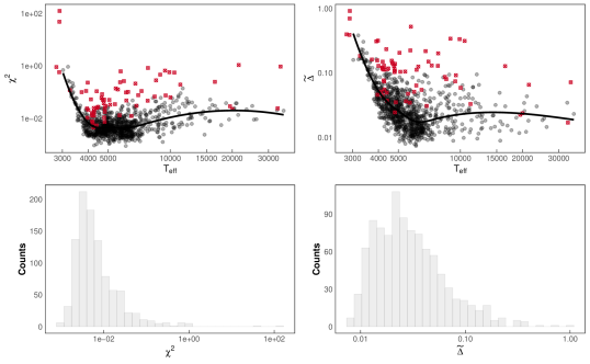
Figure 1: Top panels: The $\chi^{2}$ and $\tilde{\Delta}$ metrics as a function of $T_{\rm eff}$ for the SynCoMiL stars. Red crosses indicate stars which have not been used in the SPS models (see text in Section 2). The smooth line corresponds to a LOESS (locally estimated scatter plot smoothing) regression to the points, plotted to aid the eye. Bottom panels: Distribution of $\chi^{2}$ and $\tilde{\Delta}$ values for the SynCoMiL library.

2 SynCoMiL: A synthetic counterpart to the MILES library

For the present work we built a Synthetic Counterpart to the MILES Library (SynCoMiL hereafter), a theoretical spectral grid which mimics the MILES stellar library in terms of its wavelength and HRD coverage, and spectral resolution. MILES (Sánchez-Blázquez et al., 2006; Cenarro et al., 2007) is a carefully flux-calibrated empirical spectral library widely used in stellar population modelling (e.g. Vazdekis et al., 2010, 2012; Vazdekis et al., 2015; Vazdekis et al., 2016; Martín-Hernández et al., 2010; Maraston & Strömbäck, 2011; Röck et al., 2016). It contains spectra for close to 1000 stars covering $\lambda\lambda$ 3540 – 7410 Å at FWHM $\sim$ 2.5 Å spectral resolution (Falcón-Barroso et al., 2011). Atmospheric parameters for the stars in MILES were first compiled from the literature by Cenarro et al. (2007). Prugniel et al. (2011) and Sharma et al. (2016) re-derived these parameters, providing error estimates for the majority of the MILES stars. MILES was designed to have an optimal coverage of the HRD in terms of the effective temperature $T_{\rm eff}$, surface gravity $\log g$, and metallicity [Fe/H] of the stars in the library. The [Fe/H] vs. [$\alpha$/Fe] relation for the MILES stars, characterised by Milone et al. (2011), made the library particularly suitable for comparison with stellar spectral models, where both the abundance pattern and the global metallicity need to be defined.

It is well known that atomic and molecular opacities play an essential role in stellar atmosphere models and corresponding synthetic spectra. An analysis of libraries from the literature shows different predictions for spectral indices, depending on the exact combination of opacities and grid (e.g. Martins & Coelho, 2007). The authors illustrate a trend with $T_{\rm eff}$ (hot stars are better reproduced on average than cool ones) and wavelength (redder spectral indices being on average better reproduced than bluer ones). The recent work by Knowles et al. (2019, see their fig. 16) shows that modern grids still show evidence for a light trend with wavelength, and their differential predictions also differ. Nonetheless, and even though improving the opacities is a slow and time-consuming process, considerable progress has been achieved over time (e.g. Peterson & Kurucz, 2015; Kurucz, 2017; Franchini et al., 2018). The recent work by Martins et al. (2019) compared the ability of different grids (both empirical and synthetic) in reproducing the integrated spectra of globular clusters. They show that current synthetic grids are competitive, despite still showing discrepancies when compared to observations. Martins & Coelho (2017) discuss current needs regarding synthetic libraries, in particular for applications to stellar population studies.

The computation of SynCoMiL is largely based on the work by Coelho (2014) (C14 hereafter). Comparisons with MILES library stars discussed in C14 (see her table 6 and fig. 10) show trends with $T_{\rm eff}$ and wavelength similar to the ones mentioned above. The ingredients for these models are summarised below, and we refer the reader to C14 for technical details.

1. Opacity distribution functions (ODFs) were adopted from C14 for iron abundances [Fe/H]  = –1.3, –1.0, –0.8, –0.5, and from Castelli & Kurucz (2003) for [Fe/H]  = –3.0, –2.5, –2.0, –1.5, –0.3, –0.2, –0.1, +0.0, +0.2, +0.3, +0.4, +0.5, +1.0. A new set of ODFs was computed with [Fe/H] = –0.5 and [$\alpha$/Fe] = +0.2.

2. Model atmospheres were computed with ATLAS9 (Kurucz, 1970; Sbordone et al., 2004) for stars with $T_{\rm eff}$ $\geq$ 3500 K and the ODFs described above, adopting the atmospheric parameters of the MILES stars and the convergence criteria as in Mészáros et al. (2012); For stars with $T_{\rm eff}$ $<$ 3500 K we used existing MARCS atmosphere models (Gustafsson et al., 2008) to compute a small grid of cool stars. In all MARCS models we adopted the standard chemical composition class, with spherical model geometry for $\log g$ $\leq$ 1.5, and plane-parallel for $\log g$ $\geq$ 4.5.

3. Synthetic stellar spectra were computed with the SYNTHE code (Kurucz & Avrett, 1981; Sbordone et al., 2004), based on the ATLAS9 and MARCS models. The opacities are as in C14 with one update, the inclusion of the molecular transition C₂ D-A from Brooke et al. (2013) to correct for the problem identified by Knowles et al. (2019). For stars with $T_{\rm eff}$ $\geq$ 3500 K the synthetic spectrum was computed based on the ATLAS9 models. Cooler star spectra were computed from the MARCS model grids, then interpolated to achieve the atmospheric parameters of SynCoMiL stars. Interpolation was performed linearly in $\theta=5040$/$T_{\rm eff}$, $\log g$ and [Fe/H], with the flux in logarithmic scale. We adopted this scheme after different tests comparing synthetic spectra with the interpolated ones.

4. The synthetic spectra were then corrected for the effect of predicted lines, interpolating linearly the coefficients listed in Table B1 of C14 to the exact atmospheric parameters of the SynCoMiL stars.

5. The spectra were convolved, rebinned and trimmed to match the resolution, dispersion and wavelength range of MILES (Falcón-Barroso et al., 2011).

We adopt the MILES atmospheric stellar parameters mainly from Prugniel et al. (2011), with the revision for cool stars provided by Sharma et al. (2016). For 26 stars we use the parameters from Cenarro et al. (2007), either because Prugniel et al. (2011) do not provide an independent determination, or because we concluded by visual comparison that the Cenarro et al. (2007) parameters permit a closer match between observed and model spectra. For stars HD001326B and HD199478 we modified slightly the reported parameters, as we could not obtain converged models for the nominal parameters. The changes in $T_{\rm eff}$ and $\log g$ are nevertheless small – the smallest needed to achieve convergence – and are within the reported errors. We list in Table 1 the atmospheric parameters adopted for each star in MILES and SynCoMiL, along with their respective sources. To mimic the abundance pattern of the MILES library, we follow table 7 of C14, based on the work by Milone et al. (2011).

Table 1: Atmospheric parameters used as input values in the computation of SynCoMiL (abridged; the full table is available as supplementary online material; see Table LABEL:tab_atmpars). Unlisted MILES stars are not used in the SPS models in this work and are reported separately in Table 2 (see Section 2).

MILES ID	Star	$T_{\rm eff}$	$\log g$	[Fe/H]	Notes
001	HD224930	5411	4.19	-0.78	b
002	HD225212	4117	0.68	0.14	c
012	HD001326b	3571	4.81	-0.57	d
096	HD016901	5345	0.85	0.00	a
149	HD027371	4995	2.76	0.15	b
581	HD143807	10727	3.84	-0.01	b
Atmospheric parameters adopted from: aCenarro et al. (2007);
bPrugniel et al. (2011); cSharma et al. (2016); dUsed different
parameters than proposed in the literature to ensure model
convergence.

Table 2: MILES stars unsuitable for SPS modelling (abridged; the full table is available as supplementary online material; see Table LABEL:tab_discarded).

MILES ID	Star	$T_{\rm eff}$	$\log g$	[Fe/H]	Notes
029	HD004395	5444	3.43	-0.27	b, 1, 6
044	HD006474	6781	0.49	0.26	b, 6, 7
045	HD006497	4401	2.55	0.00	c, 1, 6
104	HD018391	5750	1.20	-0.13	b, 5, 6, 7
140	HD281679	8542	2.50	-1.43	a, 6
204	HD041117	20000	2.40	-0.12	b, 3
212	HD043042	6480	4.18	0.06	b, 2
246	HD055496	4858	2.05	-1.48	b, 4
780	HD199478	11200	1.90	0.00	d, 3, 6
Atmospheric parameters adopted from: aCenarro et al. (2007);
bPrugniel et al. (2011); cSharma et al. (2016); dsame as a but
unknown [Fe/H] assumed to be solar. Star discarded due to:
1Excessive noise or corrupted spectrum; 2Visible continuum
distortions; 3Visible emission lines; 4Peculiar features;
${}^{5}E(B-V)>0.3$ from Prugniel et al. (2011); 6Removed by cut
in $\chi^{2}$; 7Removed by cut in $\tilde{\Delta}$ (Section 2).

SynCoMiL spectra were compared with the empirical ones from MILES both visually and quantitatively. Quantitative differences between model and observations were obtained via a $\chi^{2}$ metrics

$$\chi^{2}=\sum_{\lambda}{\frac{\left(f^{\textrm{syn}}_{\lambda}-{f^{\textrm{obs}}_{\lambda}}\right)^{2}}{\sigma^{2}_{\lambda}}},$$ (1)

and a median deviation $\tilde{\Delta}$ defined as

$$\tilde{\Delta}={\rm median}\left({\frac{|f^{\textrm{syn}}_{\lambda}-f^{\textrm{obs}}_{\lambda}|}{f^{\textrm{obs}}_{\lambda}}}\right),$$ (2)

where $f^{\textrm{syn}}_{\lambda}$ and $f^{\textrm{obs}}_{\lambda}$ are the synthetic and observed fluxes at a given $\lambda$, respectively. The standard deviation $\sigma_{\lambda}$ appearing in Eq. (1) was estimated for each star as follows. P. Sánchez-Blázquez (priv. comm.) kindly provided us with the error spectra for each star in MILES, which was used in turn to compute the signal-to-noise ratio SNR($\lambda$) for each star. Since very deviant values of SNR were obtained for some of the stars, we chose to use the median[SNR($\lambda$)] of the distribution of SNR at each $\lambda$ as a fiducial value to compute $\sigma_{\lambda}=f^{\textrm{obs}}_{\lambda}$/median[SNR($\lambda$)]. This fiducial SNR($\lambda$) ranges from $\approx 8$ to $\approx 190$ over the MILES wavelength range.

Fig. 1 shows the resulting distributions of $\chi^{2}$ and $\tilde{\Delta}$, as well as the corresponding values for each star plotted vs. $T_{\rm eff}$. We found that $T_{\rm eff}$ is the only atmospheric parameter which correlates with the metrics in Eqs. 1 and 2. The patterns in Fig. 1 are in agreement with previous work: the larger values of $\chi^{2}$ and $\tilde{\Delta}$ for cool stars are in agreement with, e.g., Martins & Coelho (2007) and C14, and the larger values for $T_{\rm eff}$ $\gtrapprox$ 7000K are consistent with the larger errors in $T_{\rm eff}$ for these stars reported by Prugniel et al. (2011). The red symbols in 1 correspond to 71 stars which we opted not to use in the remaining of this work (e.g., bottom panel in Fig. 2). Spectra in MILES which are not suitable for stellar population modelling have been identified previously in the literature (e.g., Prugniel et al., 2011; Barber et al., 2014, R. Peletier, priv. comm.). In the present work, a star is not used in the SPS models if any of the conditions below applies.

1. The observed spectrum shows:

   • emission lines,

   • excessive noise or corrupted pixels,

   • distortions in the continuum,

   • $E(B-V)$ > 0.3, as inferred by Prugniel et al. (2011),

   • peculiar spectral features (e.g. HD055496).

2. $\chi^{2}$ and $T_{\rm eff}$ fulfill any of:

   • $T_{\rm eff}$ < 4000 K and $\chi^{2}>1$,

   • 4000 $\leq$ $T_{\rm eff}$ $\leq$ 7000K and $\chi^{2}>0.05$,

   • $T_{\rm eff}$ > 7000 K and $\chi^{2}>0.15$.

3. $\tilde{\Delta}$ and $T_{\rm eff}$ fulfill any of:

   • $T_{\rm eff}$ $<$ 4000K and $\tilde{\Delta}>0.4$,

   • $T_{\rm eff}$ $\geq$ 4000K and $\tilde{\Delta}>0.1$.

Table 2 lists the discarded stars. Most of the discarded stars satisfy more than one of these criteria. Stars which fall into the quantitative cuts listed above show strong continuum mismatches between model and observations. We hypothesise that these are due to either large errors in $T_{\rm eff}$, or problems with flux calibration, reddening, or star identification. The results of Prugniel et al. (2011) and Martins et al. (2019) also show evidence of residual flux calibration problems in MILES. For illustration purposes, in Fig. 2 we compare model and observed spectra for three stars.

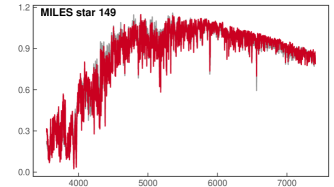
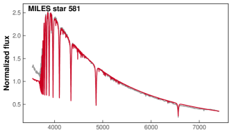
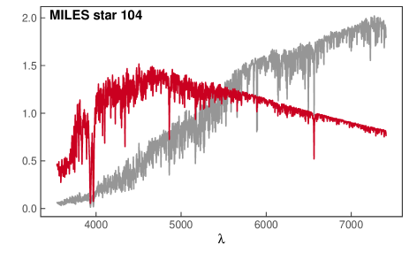
Figure 2: Comparison of MILES and SynCoMiL spectra for 3 stars in the MILES library. (top) star 149, HD027371, $T_{\rm eff}$ = 4995 K, $\log g$ = 2.76, [Fe/H] = 0.15, (middle) star 581, HD143807, $T_{\rm eff}$ = 10727 K, $\log g$ = 3.84, [Fe/H] = -0.01, and (bottom) star 104, HD018391, $T_{\rm eff}$ = 5750 K, $\log g$ = 1.20, [Fe/H] = -0.13. The indicated atmospheric parameters are taken from Prugniel et al. (2011). MILES spectra are shown in gray and SynCoMiL spectra are shown in red. Fluxes have been normalised to $\int_{3540}^{7410}{F_{\lambda}\,d\lambda}=1$. The top and middle panels show SynCoMiL stars around the 25th and 50th percentiles of the $\tilde{\Delta}$ distribution in Fig. 1. The bottom panel shows a ‘peculiar‘ case, identified as a Cepheid variable by Prugniel et al. (2011), discarded from the remaining of the present work. See Section 2 and Tables 1 and 2.

3 Methodology

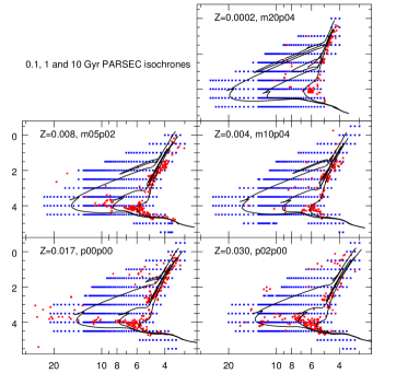
Figure 3: Coverage of the stellar flux libraries in the $\log g$ vs. $T_{\rm eff}$ diagram. Red symbols indicate the MILES (and SynCoMiL) stars, and the blue symbols represent the stars from C14. Isochrones for ages 0.1, 1 and 10 Gyr are plotted as black lines. The chemical mixtures are indicated in each panel (see Table 3).

Table 3: Metallicity regimes explored in the present work

Bin	Isochrone	[Fe/H]	# MILES	C14a
	$Z$	range	stars	mix
Sub Solar 3	0.0002	$<-1.3$	86	m20p04
Sub Solar 2	0.004	$[-1.3,-0.6]$	144	m10p04
Sub Solar 1	0.008	$[-0.6,-0.1]$	262	m05p02
Solar	0.017	$[-0.1,+0.1]$	224	p00p00
Super Solar 1	0.030	$>+0.1$	198	p02p00
a Extended for the present work by adding the mixtures
([Fe/H], [$\alpha$/Fe]): (–2.0, 0.4) and (–0.5, 0.2), corresponding to
$Z=0.0002$ and $0.008$.

To address the questions outlined in Section 1, we compute four different sets of SPS models in which all the ingredients are the same except for the choice of the stellar flux library. The SPS models are computed using the galaxev code (Bruzual & Charlot, 2003, and recent updates). This is a flexible code which provides SPS models for a variety of stellar evolutionary tracks, stellar spectral libraries, chemical abundances, initial mass functions, and star formation histories, and probes ideal towards our goal of computing models which differ only in the stellar spectral library. We adopt the PARSEC stellar evolutionary tracks (Bressan et al., 2012; Chen et al., 2015) to describe the evolution of stellar populations of the five metallicities listed in Table 3. From the evolutionary tracks the galaxev code builds isochrones for the required age and metallicity.

Fig. 3 shows three isochrones for each stellar metallicity in Table 3, together with the coverage in the HRD of the MILES, SynCoMiL, and C14 libraries. This coverage is complete for C14 but very sparse for MILES. The sparse coverage of the HRD by the MILES and other empirical libraries is what forces us to supplement these libraries with synthetic stellar spectra in the Bruzual & Charlot (2003, and recent updates) models. One of the goals of the present paper is to quantify the effects on the SPS models of assigning stellar spectra with ($T_{\rm eff}$, $\log g$, [Fe/H]) relatively far from the true values.

We consider four different sets of SPS models for each mixture in Table 3, denoted sps-m, sps-s, sps-c and sps-r, which differ only in the stellar spectral library, as follows:

sps-m: the empirical MILES library.

sps-s:  the synthetic SynCoMiL library.

sps-c:  the synthetic C14 library.

sps-r:  10 realisations of sps-s  (details below).

To each star along an isochrone, the galaxev code assigns a spectrum drawn from the selected library. The stellar spectrum is assigned on the basis of the proximity of the stellar parameters of the library stars to the corresponding parameters of the problem star in the HRD, interpolating between neighbouring spectra when required. For the sps-c models, each problem star in the isochrone is bracketed by four C14 stellar models (see Fig. 3), characterized each by ($\theta$, $\log g$), where $\theta$= $5040/T_{\rm eff}$. In this case, we interpolate the stellar models logarithmically in flux, first in $\theta$ at constant $\log g$ and then in $\log g$. This interpolation scheme is possible only in very few instances when using the MILES library in the sps-m models. In some cases, we can interpolate in $T_{\rm eff}$ two MILES spectra of the required $\log g$, but in most cases we use the MILES spectrum closest in ($T_{\rm eff}$, $\log g$) to the problem star on the isochrone.

For the sps-s models, we use the same spectral assignment as in the sps-m models, but draw the corresponding stellar spectra from the SynCoMiL instead of the MILES library.

For the sps-r models, we modify the stellar parameters of each SynCoMiL star by adding to each parameter a Gaussian random error. Then we replace each star in the sps-s models with the star with closest parameters in the modified table. This exercise is repeated 10 times for each set of SPS models listed in Table 3. We adopt errors for $T_{\rm eff}$ and $\log g$ as compiled by C14 (see her table 5): for $T_{\rm eff}$ the error ranges from 120 K for cool stars to 3000 K for hot stars; for $\log g$ the errors range from 0.1 to 0.3 depending on $T_{\rm eff}$. For [Fe/H] we adopt conservative errors of 0.15 (e.g., Soubiran et al., 1998).

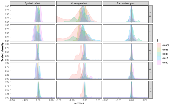
Figure 4: Density plots showing the distributions of colour differences ($\Delta{\rm\sf colour}$, defined in Section 4.1.1) for the different combinations of SDSS-based colours (in rows) and the model effects (in columns). Colours indicate the metallicities Z, as indicated in the label.

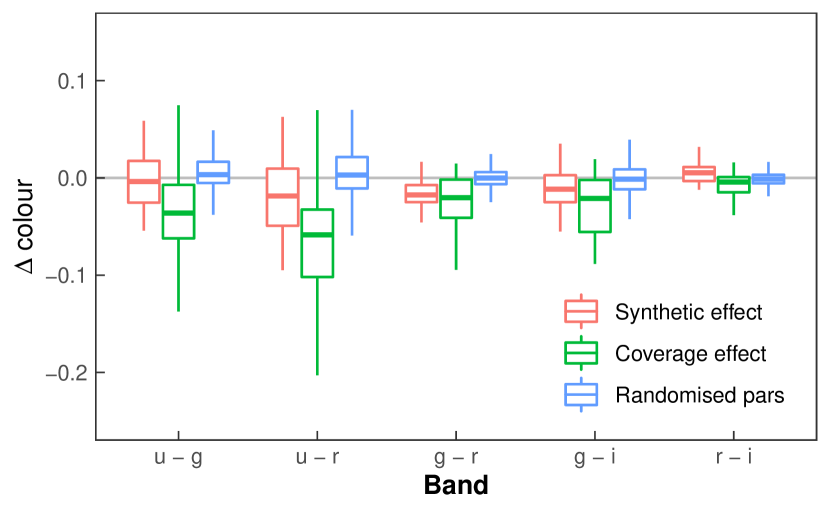
Figure 5: The values of $\Delta{\rm\sf colour}$ are given for each color (x-axis) and effect (coloured labels). Each box indicates the range from the 25% to the 75% percentiles, with the horizontal line indicating the median value. The whiskers have length equal to $\pm 1.5\times$IQR. Outliers are not shown.

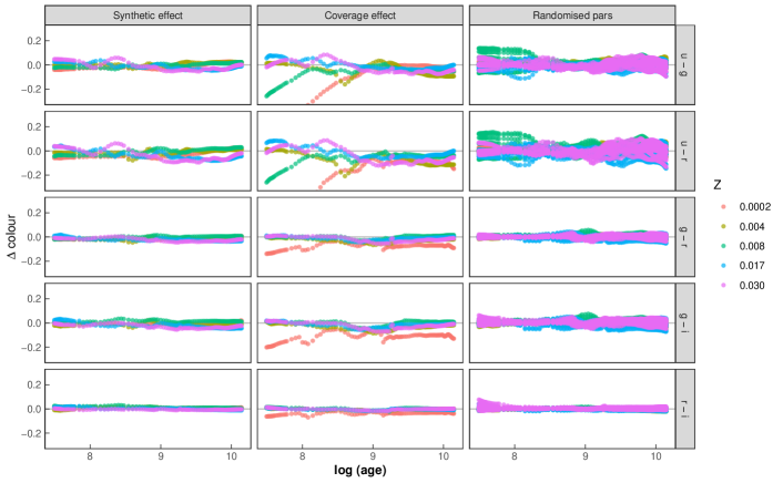
Figure 6: $\Delta{\rm\sf colour}$ differences for the three effects (columns) described in Section 4.1, plotted as a function of stellar population age (in yr). Different colours are shown in rows, and different metallicities are identified as indicated in the label.

4 Results

The different SPS models described in Section 3 were compared to each other in two ways: (1) via direct model – model comparisons (Section 4.1), and (2) using the models to derive stellar population parameters via spectral fits to a sample of galaxy spectra (Section 4.2).

4.1 Model – model comparisons

From the direct comparison of the colours and spectral line indices predicted by the different models we aim at understanding the following three effects:

Synthetic effect: comparing the predictions of the sps-m and sps-s models we can assess the consequences of using theoretical instead of empirical stellar spectra for a fixed coverage of the HRD.

Coverage effect: comparing the predictions of the sps-s and sps-c models we can isolate the consequences of limited vs. complete HRD spectral coverage on the observables.

Random error effect: comparing the sps-r and sps-s models, we can assess the effects of random errors in the stellar atmospheric parameters on the model predictions.

4.1.1 Broad-band colors

For each set of models, we compute 5 colours, $u-g$, $u-r$, $g-r$, $g-i$, and $r-i$, using the SDSS $ugri$ filter response functions (Doi et al., 2010). For each age and metallicity of the SPS models we compute the following colour differences in direct relation to the effects listed above:

$$\Delta{\rm\sf colour}_{\rm Synthetic}={c}_{\textsc{sps-m}}-{c}_{\textsc{sps-s}},$$ (3a)

$$\Delta{\rm\sf colour}_{\rm Coverage}={c}_{\textsc{sps-c}}-{c}_{\textsc{sps-s}},$$ (3b)

$$\Delta{\rm\sf colour}_{\rm RanError}={c}_{\textsc{sps-r}}-{c}_{\textsc{sps-s}},$$ (3c)

where $c$ is a colour. Results are shown in Figs. 4, 5 and 6, and listed in Table 4.

Fig. 4 shows the distributions of $\Delta{\rm\sf colour}$ for the different colours (rows) and effects (columns). We notice that the distributions are not always symmetric, and that they are typically broader for the coverage effect than for the synthetic and randomised-parameter effects. These results are illustrated in a condensed manner as a boxplot in Fig. 5, indicating the corresponding median and interquartile range (IQR) given in Table 4. In Fig. 6, we show $\Delta{\rm\sf colour}$ as a function of stellar population age for the different colours and effects. A large variance in colours involving the $u$ band arises at ages younger than 1 Gyr, especially at low metallicity, which is not surprising given the limited number of hot metal poor stars in empirical libraries.

In summary, the coverage effect dominates the systematics and variance in $\Delta{\rm\sf colour}$. The most affected colours are those involving the $u$ band, and the largest $\Delta{\rm\sf colour}$ is $\Delta(u-r)_{\rm Coverage}=0.06$.

Table 4: Median and IQR values of $\Delta{\rm\sf colour}$ in magnitude units.

Colour	Synthetic		Coverage		Random error
	effect		effect		effect
	(sps-m –sps-s)		(sps-c – sps-s)		(sps-r – sps-s)
	Median	IQR	Median	IQR	Median	IQR
$u-g$	–0.002	0.043	-0.038	0.068	0.003	0.021
$u-r$	–0.018	0.059	-0.061	0.085	0.001	0.031
$g-r$	–0.017	0.017	-0.018	0.043	0.001	0.011
$g-i$	–0.009	0.035	-0.017	0.062	–0.001	0.020
$r-i$	0.007	0.019	-0.003	0.017	–0.001	0.009

4.1.2 Spectral indices

Table 5: Spectral indices measured in the present work.

Indices	Reference
H10, H9, H8	Marcillac et al. (2006)
HK	Brodie & Hanes (1986)
B4000	Kauffmann et al. (2003)
H$\delta$A, H$\delta$F, H$\gamma$A, H$\gamma$F	Worthey & Ottaviani (1997)
CN1, CN2, Ca4227, G4300,	Trager et al. (1998)
Fe4383, Ca4455, Fe4531,
Fe4668, Hβ, Fe5015, Mg1,
Mg2, Mgb, Fe5270, Fe5335,
Fe5406, Fe5709, Fe5782, NaD,
TiO1, TiO2

The spectral indices listed in Table 5 were measured in all SPS models. We define $\Delta{\rm\sf idx}$ as the index difference between two sets of models:

$$\Delta{\rm\sf idx}_{\rm Synthetic}={I}_{\textsc{sps-m}}-{I}_{\textsc{sps-s}},$$ (4a)

$$\Delta{\rm\sf idx}_{\rm Coverage}={I}_{\textsc{sps-c}}-{I}_{\textsc{sps-s}},$$ (4b)

$$\Delta{\rm\sf idx}_{\rm RanError}={I}_{\textsc{sps-r}}-{I}_{\textsc{sps-s}},$$ (4c)

where $I$ is any spectral index. We measure $\Delta{\rm\sf idx}$ for all ages and metallicities. Results are shown in Figs. 7 – 11, and listed in Table 6.

Fig. 7 shows the distributions of $\Delta{\rm\sf idx}$ for each index. The impact of the three effects on the indices is complex and defies simple conclusions. In all cases, the effect of the random errors on the atmospheric parameters is the least important. The indices for which the synthetic effect is most prominent are: CaHK, Fe4668, Fe5270, Fe5709 and NaD. The impact of HRD coverage in the indices is not negligible and dominates over the synthetic effect in the case of, e.g., H8, B4000, and G4300. For many indices the synthetic and coverage effects are comparable and may introduce different systematic effects. Table 6 lists the median and IQR values of $\Delta{\rm\sf idx}$ for each index and effect.

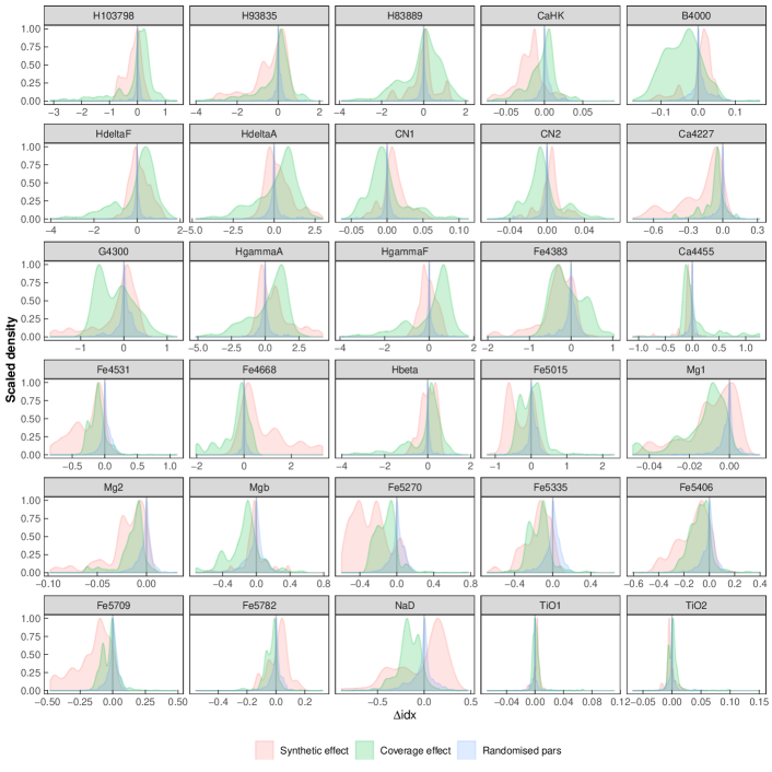
Figure 7: Density plots showing the distributions of index differences ($\Delta{\rm\sf idx}$, as defined in Section 4.1.2) for the indices listed in Table 5. The different effects are shaded as indicated in the label.

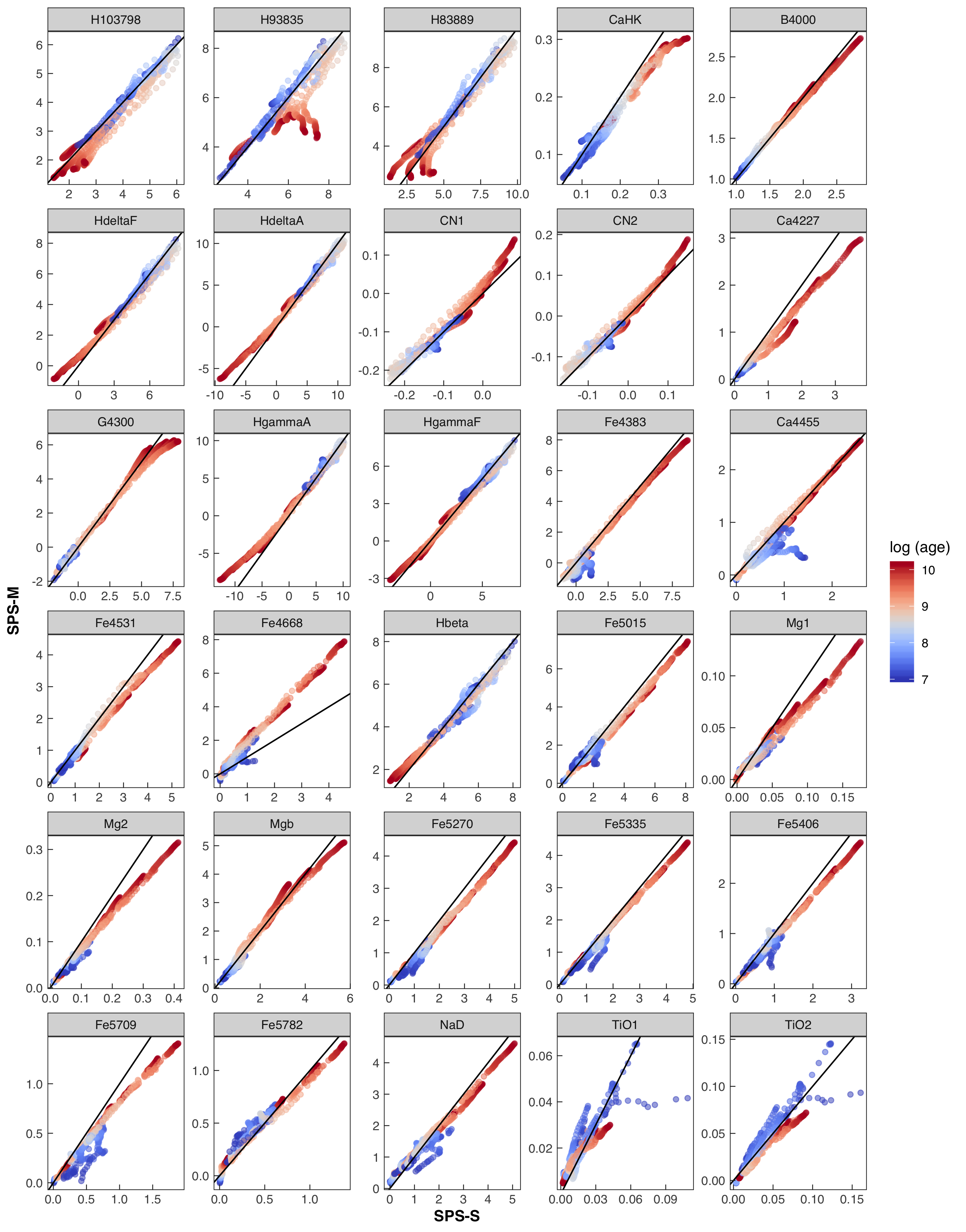
Figure 8: Spectral indices predicted by sps-m (y-axis) vs. sps-s (x-axis) models. The points are colour-coded by the age of the population, as indicated by the auxiliary axis.

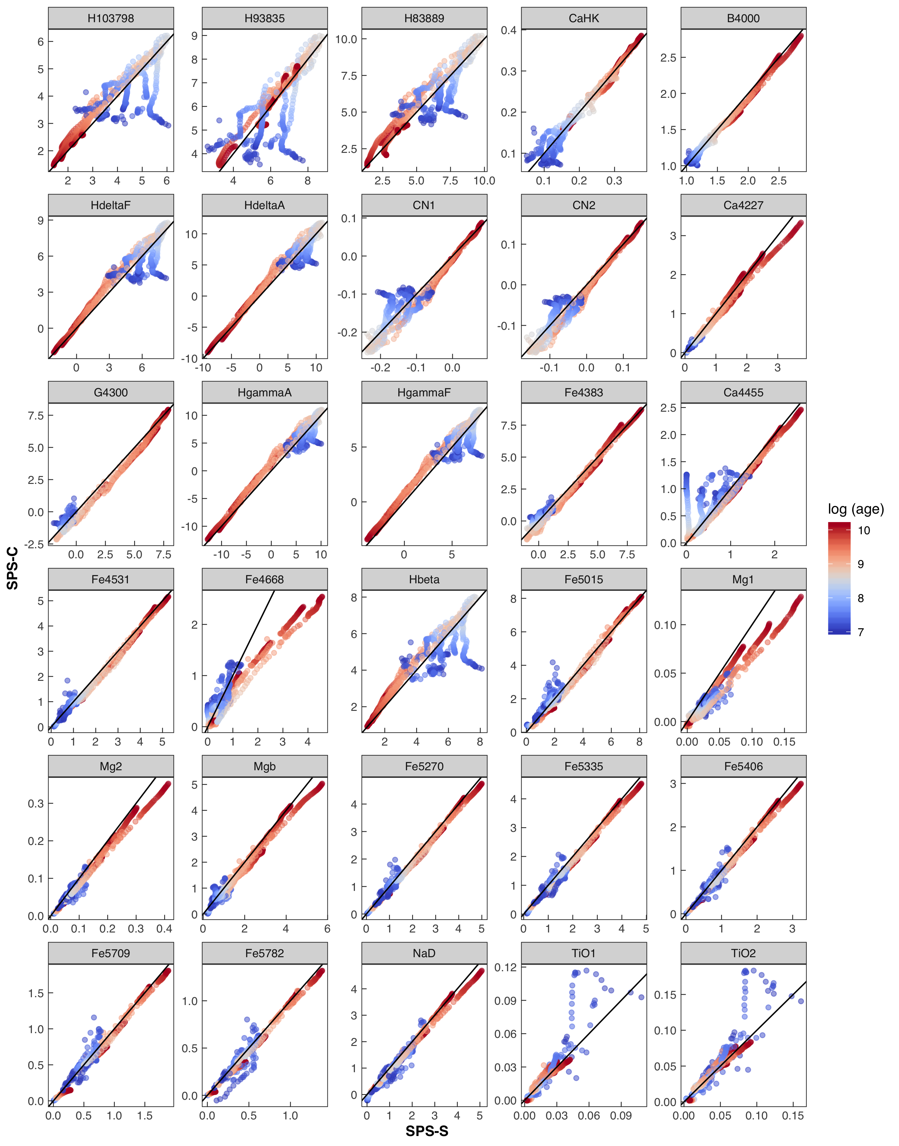
Figure 9: Spectral indices predicted by sps-c (y-axis) vs. sps-s (x-axis) models. The points are colour-coded by the age of the population, as indicated by the auxiliary axis.

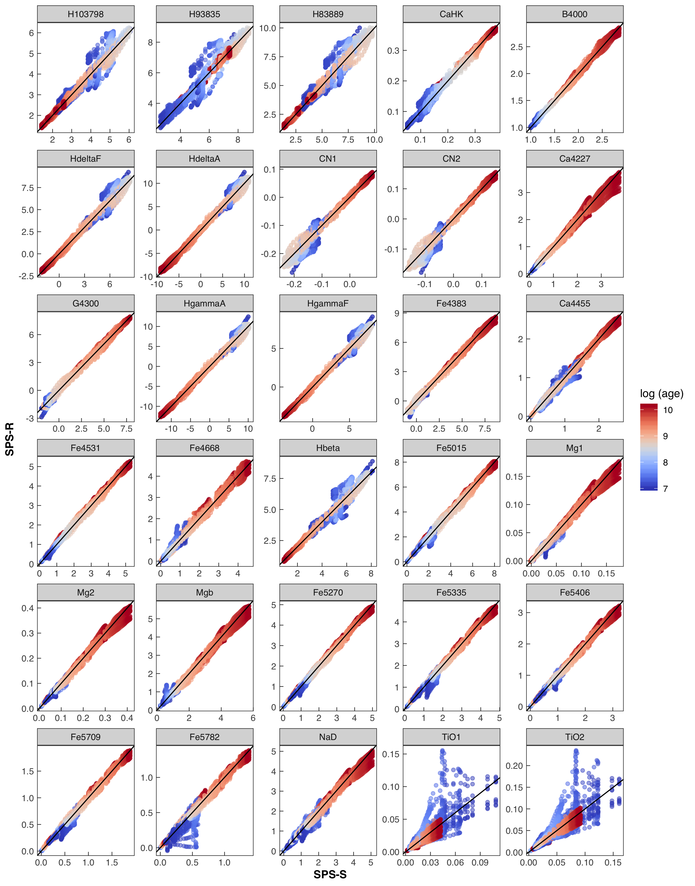
Figure 10: Spectral indices predicted by sps-r (y-axis) vs. sps-s (x-axis) models. The points are colour-coded by the age of the population, as indicated by the auxiliary axis.

Table 6: Median and IQR values of $\Delta{\rm\sf idx}$.

Index	Synthetic		Coverage		Random error
	effect		effect		effect
	(sps-m –sps-s)		(sps-c – sps-s)		(sps-r – sps-s)
	Median	IQR	Median	IQR	Median	IQR
H103798	-0.093	0.365	0.116	0.399	0.005	0.081
H93835	-0.154	0.997	0.088	0.730	0.017	0.151
H83889	0.046	0.472	0.068	1.095	0.003	0.159
CaHK	-0.018	0.018	0.000	0.020	0.001	0.006
B4000	0.014	0.027	-0.038	0.071	0.002	0.019
H$\delta$A	0.138	1.068	0.520	1.467	-0.006	0.250
H$\delta$F	0.052	0.568	0.242	0.903	-0.003	0.134
H$\gamma$A	0.458	1.285	0.653	1.820	-0.010	0.308
H$\gamma$F	-0.058	0.473	0.478	0.977	-0.003	0.148
CN1	0.009	0.016	-0.006	0.024	0.000	0.005
CN2	0.005	0.010	-0.006	0.017	0.000	0.004
Ca4227	-0.104	0.257	-0.052	0.070	0.001	0.037
G4300	0.014	0.439	-0.225	0.647	0.025	0.163
Fe4383	-0.288	0.450	-0.150	0.624	0.003	0.144
Ca4455	-0.071	0.072	-0.057	0.227	0.002	0.045
Fe4531	-0.181	0.370	-0.109	0.143	0.012	0.080
Fe4668	0.409	1.204	-0.150	0.622	0.011	0.081
H$\beta$	0.074	0.550	0.146	0.661	0.003	0.095
Fe5015	-0.378	0.631	0.019	0.462	0.034	0.138
Mg1	-0.006	0.015	-0.009	0.013	0.000	0.003
Mg2	-0.016	0.021	-0.011	0.012	-0.000	0.007
Mgb	-0.026	0.091	-0.112	0.184	-0.001	0.101
Fe5270	-0.294	0.248	-0.109	0.155	0.008	0.079
Fe5335	-0.131	0.179	-0.123	0.153	0.008	0.086
Fe5406	-0.101	0.179	-0.074	0.113	0.004	0.056
Fe5709	-0.114	0.162	-0.011	0.080	0.005	0.040
Fe5782	0.031	0.090	-0.025	0.056	0.003	0.032
NaD	0.084	0.393	-0.163	0.151	-0.001	0.102
TiO1	0.003	0.004	0.000	0.005	0.000	0.003
TiO2	-0.004	0.007	0.001	0.008	-0.000	0.005

In Figs. 8, 9 and 10 we plot the indices computed from sps-m, sps-c and sps-r against those of sps-s models, respectively. The dependence with the age of the population is apparent: as expected, the largest deviations from the 1-to-1 line occur for the old population in the case of the synthetic effect, and for the young population in the case of the coverage effect. In these plots we can locate opacity related problems, e.g., Fe4668 (see discussion in Knowles et al. 2019), or the high sensitivity to HRD coverage of the Balmer line indices. The effect of randomising the stellar parameters is to increase the dispersion of the data points but they do not deviate significantly from the 1-to-1 line except for young populations: most likely this is induced by the coverage effect due to the scarcity of hot stars in the HRD.

The boxplot in Fig. 11 is convenient to easily rank the sensitivity of each index to the effect being explored. To facilitate visualisation, $\Delta{\rm\sf idx}$ has been scaled to its standard score (or z-value), defined as:

$$z=\frac{x-\mu}{\sigma},$$ (5)

where $x$ is the raw $\Delta{\rm\sf idx}$ value, $\mu$ is the mean value of $x$ for the population, and $\sigma$ its standard deviation. In each panel (top: synthetic effect; middle: coverage effect; bottom: randomised parameters) the indices are sorted in increasing order of $\Delta{\rm\sf idx}$. Deviations from the zero-line indicate systematic effects and the size of the box indicates the IQR. The further away from the zero-line the midline of a box is, the more the index is affected by systematics.

In summary, the consequences of the synthetic and the coverage effects on the indices are multiple and difficult to summarise in simple terms. The outcome of randomising the stellar parameters is small compared to the other effects.

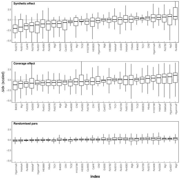
Figure 11: Boxplots of $\Delta{\rm\sf idx}$ are shown for the synthetic (top), coverage (middle) and randomised parameters (bottom) effects. In each row, $\Delta{\rm\sf idx}$  are sorted in crescent order to facilitate identification of most affected indices in each case. The values of $\Delta{\rm\sf idx}$ have been scaled to their standard score to facilitate comparison (see Section 4.1.2).

4.2 Spectral fitting of galaxies

The model – model comparisons of the previous section illustrate interesting differences between the sets of SPS models, but cannot be easily translated into the question that matters the most: how does the adoption of different spectral libraries change the age and metallicity of galaxies derived from their integrated light?

To address this question, we use the sps-m, sps-s, and sps-c models to derive stellar population parameters from the spectra of $\sim$1000 nearby galaxies ($0.04<z<0.06$). We use the sample of Gadotti (2009) which encompasses galaxies of different morphology: ellipticals, spirals (with classical or pseudo-bulges, with and without bars), and bulgeless discs. The spectra were obtained from the SDSS database (Abazajian et al., 2004) and processed as in Coelho & Gadotti (2011). We use the Starlight spectral fitting code (Cid Fernandes et al., 2005) to infer the stellar population parameters, processing the sample three times, once for each set of SPS models. We refer the reader to the quoted work for details on the sample and technique.

We show in Fig. 12 the results for two parameters related to the fit-quality and three parameters related to the stellar population. The parameters related to the fit-quality are $\chi^{2}$(as in equation 1) and an average relative deviation adev, defined as

$${\rm\sf adev}=\frac{1}{N}\sum_{\lambda}\left(\frac{|f^{\textrm{model}}_{\lambda}-f^{\textrm{obs}}_{\lambda}|}{f^{\textrm{obs}}_{\lambda}}\right),$$ (6)

where N is the number of wavelength points in the spectrum, $f^{\textrm{model}}_{\lambda}$ is the model spectrum fitted by Starlight, and $f^{\textrm{obs}}_{\lambda}$ is the observed galaxy spectrum.

The synthetic effect can be inspected in the left hand side column of Fig. 12, which compares the results from sps-m (y-axis) vs. those from sps-s (x-axis). We highlight that spectral fits performed with sps-s models tend to have larger $\chi^{2}$ and adev than those obtained with sps-m models, even though there are no noticeable differences in the retrieved values of A_V and log (age). The values of [Fe/H] obtained with the sps-s models are systematically lower than those obtained with the sps-m models. The differences in [Fe/H] correlate with [Fe/H], lower metallicities showing larger differences.

The coverage effect can be inspected in the right hand side column of Fig. 12, which shows the results from sps-c (y-axis) vs. results from sps-s (x-axis) models. We notice that spectral fits performed with the sps-s and sps-c models have similar adev, but $\chi^{2}$ is slightly larger for the sps-c fits. There are no noticeable differences in the retrieved values of Av. Whereas the values of log(age) obtained from the sps-c models are larger than for the sps-s models, there are no systematic differences in the retrieved mean [Fe/H], even though there are some outliers from the 1–to–1 line, which remain to be investigated.

Table 7 shows the median residuals and IQRs for the parameters obtained from sps-m vs. sps-s fits (synthetic effect), and sps-c vs.s sps-s fits (coverage effect). In all cases, the systematic differences are inside the IQR ranges. We note that the median residuals on [Fe/H] and log(age) are of the same order of the IQR for the synthetic effect and the coverage effect, respectively.

Table 7: Median residuals and IQR for spectral fits

Parameter	Synthetic effect		Coverage effect
	(sps-m – sps-s)		(sps-c – sps-s)
	median	IQR	median	IQR
$\chi^{2}$	–0.05	0.13	0.04	0.06
adev	–0.16	0.29	0.09	0.10
AV	0.00	0.04	0.01	0.05
mean $\log{\rm(age)}$	0.00	0.12	0.11	0.14
mean [Fe/H]	0.13	0.13	–0.01	0.12

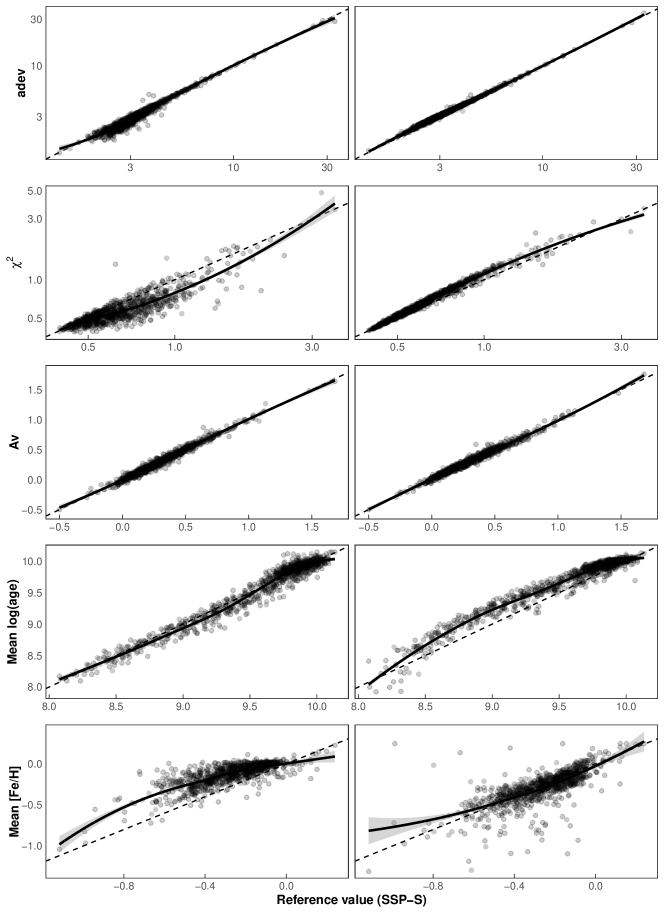
Figure 12: Results from the spectral fitting of a sample of nearby galaxies. The left-side column shows the results obtained from sps-m (y-axis) vs. sps-s (x-axis) models. The right-side column shows the results obtained from sps-c (y-axis) vs. sps-s (x-axis) models. The different parameters inferred are given in rows: $\chi^{2}$, adev (Eq. 6), reddening Av, light-weighted log(age), and light-weighted [Fe/H]. The smooth line corresponds to a LOESS (locally estimated scatterplot smoothing) regression to the points and is shown to guide the eye.

5 Discussion

5.1 Semi-empirical vs. theoretical SPS models

How do uncertainties in theoretical stellar libraries affect integrated colours and line indices measured in SPS models?

Several works in the literature compare synthetic stellar spectra to empirical ones on a star-by-star basis (e.g. Martins & Coelho, 2007; Bertone et al., 2008). Recent work by Martins et al. (2019) provides insight into how synthetic vs. empirical spectra compare at the level of the integrated properties of stellar populations. These authors model integrated spectra of clusters combining CMDs and stellar libraries from different sources. Their conclusions depend on the wavelength range. From 3900 to 6300 Å, or when considering specific spectral features, empirical libraries do better. In the range 3525 to 6300 Å, a theoretical library outperformed the empirical ones in 70% of their tests, essentially because the shape of the continuum is more in agreement with the observations in the theoretical case.

Our results add more information to the theoretical vs. empirical library debate. The SPS models built in this work are largely based on the theoretical library by C14. Her fig. 10 illustrates the systematic differences between synthetic spectra for given $T_{\rm eff}$ and $\log g$, and MILES spectra averaged over all stars in the library with the same atmospheric parameters (within uncertainties). The two main possible reasons for these differences are: either they result from abundance patterns unaccounted for in the synthetic grid (such as variations of C and N due to dredge-up in giants stars), or they reflect true deficiencies in the spectral modelling, related to either the physics of the stellar atmosphere or to the adopted atomic opacities. In the present analysis we assume that all differences are due to the opacities.

In Section 4.1, colours and spectral indices from the sps-m and sps-s models were compared to quantify how the inaccuracies in the opacities translate into the integrated light of the stellar population. The results from Table 4 show that the systematic effect on broad-band colours ranges from $-0.002$ in $u-g$ to $-0.018$ in $u-r$. The IQR of the distributions range from 0.017 in $g-r$ to 0.059 in $u-r$. For comparison, the reported accuracy (global rms dispersion) of the flux calibration for the MILES library is 0.013 mag in $B-V$.

Comparing the spectral indices we get a closer view of the role played by the opacities. Figs. 7, 8 and 11 show a complex and index-dependent behaviour. One may argue that the best performance of the sps-s models occurs for the indices H10, B4000, H$\delta_{F}$, CN₂, G4300, H$\gamma_{F}$, Fe4383, H$\beta$, Mg_b and Fe5782, whereas the indices that deserve most attention from modellers are Fe5270, Fe5015, CaHK, Fe5709, Fe4383 and Fe4668 (the latter had already been pointed out by Knowles et al. 2019).

It is unclear to what extent the results presented here can be safely applied to other theoretical libraries. Given that the broad-band colours depend mostly on averaged opacities and on the physics of the stellar atmosphere, we expect the results for the colours to be similar for other modern libraries of statistical fluxes (e.g. Gustafsson et al., 2008; Castelli & Kurucz, 2003), or in high-resolution spectral libraries as long as the effect of predicted lines has been taken into account (see discussion in section 3 of C14). On the other hand, the results for the spectral indices depend on the details of the specific opacities, and it is less likely that they can be reliably adopted for other synthetic libraries. As such, the reader should see our results on the spectral indices as guidelines for the use of the C14 library.

5.2 The effect of the HRD coverage

How does the non-ideal or poor coverage of the HRD by empirical libraries affect the predictions of SPS models?

Empirical libraries cannot cover the HRD homogeneously and completely due to observational constrains. We do not harbour in our Galaxy massive metal-poor stars, which are likely to be present in high redshift galaxies, nor can we cover the abundance patterns of galaxies with diverse star formation and chemical enrichment histories. By construction, with semi-empirical SPS models we can reproduce to a better degree the properties of populations similar to the solar neighbourhood than others.

Vazdekis et al. (2010) discuss this issue in the context of three empirical libraries MILES, STELIB (Le Borgne et al., 2003), and Lick/IDS (Worthey et al., 1994). They define the quality parameter $Q_{n}$ to quantify the reliability of their semi-empirical SPS models as a function of age, metallicity and IMF (see their Section 3.2). The authors conclude that the minimum age at which a model is reliable ranges from 60 Myr around solar metallicity to 10 Gyr in the most metal-poor regime, with a varying degree of quality $Q_{n}$.

Here we retake this discussion comparing our sps-s and sps-c models: the first mimics the HRD coverage of an empirical library, and the second covers the HRD completely and homogeneously for populations older than 30 Myr (cf. Fig. 3). Differences found in this experiment will be due to the incomplete HRD coverage of the empirical library, since SynCoMiL and C14 share the same codes and opacities.

The effects that the different HRD coverage have on colours can be seen in Figs. 4, 5 and 6, and are summarised in Table 4. For all colours, except $r-i$, the coverage effect introduces systematic differences and variances larger than the synthetic effect. The largest difference occurs in $u-r$, with a systematic value of $-0.061$ and IQR of 0.085. The effect is largest in the most metal-poor regime, in accordance with the results of Vazdekis et al. (2010). This is expected since the coverage of the HRD is poorest at the lowest metallicities.

The effects on spectral indices are shown in Figs. 7, 9, and 11, and are difficult to generalise. Some indices seem to be little affected (at least in comparison to the other effects) such as Fe5709 and Fe5782, while in other cases, such as B4000, the difference is prominent. Fig. 11 shows that the most affected indices are, at one extreme, B4000 and Mg1 (sps-s models, on average, underestimate the indices), and, at the other extreme, H$\delta$ and H$\gamma$ (sps-s models, on average, overestimate the indices).

5.3 Errors in the atmospheric parameters

How do errors in the stellar atmospheric parameters translate into SPS models?

Percival & Salaris (2009) performed an interesting investigation on the possible impact of systematic uncertainties in the atmospheric parameters on the integrated spectra of stellar populations. These authors simulated a systematic difference between the $T_{\rm eff}$ scale of the isochrones and that of the stellar flux libraries, and considered errors within the typical offsets found in the literature (100 K in $T_{\rm eff}$, 0.25 in $\log g$ and 0.15 in [Fe/H]). Their results raised a caution, by showing that small systematic differences between the atmospheric parameter scales can mimic non-solar abundance ratios or multiple populations in the analysis of integrated spectra. If this result is confirmed, much of what the community is concluding in terms of abundance patterns in galaxies can be an artefact, due to offsets between parameter scales and not truly a tracer of different chemical evolution.

At the suggestion of the referee, we compare our results to Percival & Salaris (2009). See their tables 1 and 2, where these authors show the impact of their tests on Lick indices for 2 choices of SSPs. In Table 8, we list $\tilde{\Delta}$idx and IQR($\Delta$idx) from our experiments for the same choices of age, metallicity and indices as in Percival & Salaris (2009). The effect of random errors on the stellar parameters is typically smaller than the effect introduced by adding a systematic difference of 100 K in the $T_{\rm eff}$ scale, and of comparable magnitude to the effect of adding systematic differences in $\log g$ and [Fe/H] of 0.25 and 0.15, respectively. The exact reason why a systematic difference in the $T_{\rm eff}$ scale has a larger impact than adding random errors to the stellar parameters is difficult to trace. We can hypothesise that random errors tend to cancel out, while a systematic difference in the $T_{\rm eff}$ scale is equivalent to selecting a younger (hotter) or older (cooler) isochrone when building an SSP model without changing the selection of stellar spectra.

In any case, a look at table 3 of Percival & Salaris (2009) shows that the deviations introduced by tampering with the atmospheric parameters is comparable to (or larger than) typical observational errors on the spectral indices. As such, these effects cannot be safely neglected. Here we complement this investigation with the sps-r models, simulating the effect of random rather than systematic variations in the atmospheric parameters. Our tests reveal that both in colours (Figs. 5 and 6, Table 4) and spectral indices (Fig. 7 and 11), the effect of randomising the atmospheric parameters is small compared to the other effects. We conclude then that random errors in the stellar parameters (within the uncertainties adopted here, see Section 3) are not a major source of concern for current SPS models.

Table 8: $\tilde{\Delta}$idx and IQR($\Delta$idx) for Lick indices (Z = 0.017)

	Age = 4 Gyr		Age = 14 Gyr
Index	$\tilde{\Delta}$idx	IQR($\Delta$idx)	$\tilde{\Delta}$idx	IQR($\Delta$idx)
HδF	0.101	0.071	0.041	0.059
HγF	0.131	0.086	0.090	0.196
CN1	-0.003	0.007	0.002	0.006
CN2	-0.002	0.008	0.006	0.005
Ca4227	-0.040	0.137	0.082	0.370
G4300	0.019	0.025	0.114	0.147
Fe4383	-0.166	0.316	0.174	0.264
Ca4455	-0.038	0.069	0.047	0.043
Fe4531	-0.004	0.087	0.051	0.033
Hβ	0.045	0.035	0.012	0.085
Fe5015	0.025	0.163	0.164	0.182
Mg1	-0.001	0.009	-0.002	0.018
Mg2	-0.004	0.014	0.005	0.031
Mgb	-0.154	0.121	0.153	0.387
Fe5270	-0.037	0.141	0.085	0.119
Fe5335	-0.018	0.140	0.054	0.227
Fe5406	-0.021	0.125	0.034	0.130
Fe5709	0.005	0.066	0.035	0.006
Fe5782	0.009	0.061	0.017	0.059
NaD	-0.009	0.137	0.001	0.445
TiO1	0.001	0.004	-0.001	0.006
TiO2	0.001	0.004	0.000	0.007

5.4 Inferring stellar-population parameters from integrated light

To what extent does the choice of an empirical or a theoretical library in the SPS model affect age, metallicity and reddening estimates from integrated light?

Possibly, the most important result of the experiments performed in this work is to estimate to what extent stellar population parameters – age, metallicity, reddening – derived from SPS models vary if we adopt in the model an empirical or a theoretical library. Given our current inability to have both complete coverage of the HRD with high quality stellar spectra, what should one favour: complete coverage of the HRD (theoretical library) or accurate spectra on a star-by-star basis (empirical library)?

There are several ways proposed in the literature to derive the stellar population parameters from integrated light, but for the purpose of the present paper we choose to investigate results obtained from spectral fitting. To that end we adopt the widely used code Starlight (Cid Fernandes et al., 2005) to fit a sample of nearby galaxies (Gadotti, 2009; Coelho & Gadotti, 2011). In Section 4.1 we show that the synthetic and coverage effect impact both colours and spectral features. A code such as Starlight, which fits the continuum and the spectral features together, is a good option to evaluate in a global manner how the stellar library of choice will influence the derived galaxy properties.

Results are shown in Fig. 12 and summarised in Table 7. The first noticeable feature is that the use of synthetic spectra tends to increase $\chi^{2}$ and adev for the fit, i.e., the fits tend to be statistically worse. This is not surprising, and reminds us that atomic and molecular opacities still need improvement. Nevertheless, and to some extent a surprising result, there are no important differences in the reddening or the ages derived using sps-m and sps-s models. There is only a hint that for intermediate ages (9 $\lesssim$ log(age) $\lesssim$ 9.5), the values obtained with sps-s are slightly lower than for sps-m. On the other hand, the effect of HRD coverage on inferred ages is more significant: the use of models with non-optimal HRD coverage underestimates virtually all ages, the effect being more pronounced for log(age) $\sim$ 9.0.

The effects on the derived metallicities are shown in the bottom panels of Fig. 12. sps-s models recover lower metallicites than sps-m models, with a median difference of 0.13. This result is consistent with the top-panel of Fig. 11, which shows more indices below the zero-line than around or above it. This is also in agreements with results from the literature that show that in general synthetic stellar spectra are stronger-lined than observed stellar spectra (e.g. Martins & Coelho, 2007; Coelho, 2014). There is an indication that the difference is stronger towards lower-metallicities, but the origin of this tendency is unclear. Having a complete coverage of the HRD does not seem to affect the derived mean metallicities, although the dispersion increases.

6 Conclusions

It has been traditionally accepted that SPS models tailored to study young populations favour the use of theoretical stellar libraries, due to their better HRD and wavelength coverage, while models targeting intermediate and old populations favour empirical stellar libraries, whose detailed spectral features are more reliable than in synthetic spectra.

In this paper we perform experiments with especially built SPS models to investigate and quantify the impact of the choice of stellar library type on: (i) the predicted colours and magnitudes of evolving simple stellar populations, and (ii) the inferred age, metallicity and redenning of a galaxy from spectral fits to its integrated spectrum.

We build a new synthetic stellar library which mimics the HRD coverage of a widely used empirical library (Section 2). During this exercise we identified 71 MILES stars (Table 2) whose spectra we consider not suitable for stellar population modelling, and we recommend not to use these spectra in SPS models.

We build SPS models using different stellar libraries (Section 3). We name synthetic effect the differences introduced in the SPS model predictions by using a theoretical vs. an empirical library, for identical HRD coverage. Analogously, we name coverage effect the differences introduced in the SPS models by using libraries with a limited vs. a complete HRD coverage. The results of our tests are given in Section 4, and further discussed in Section 5. The lessons learned are as follows.

In the majority of the cases the coverage effect is responsible for the larger deviations in the predicted colours, especially those involving the $u$ band, for which the lack of hot stars in the empirical library is more noticeable.

For spectral indices, the coverage and synthetic effects are comparable for most features in the wavelength range considered. Some indices are more sensitive to the synthetic effect (e.g. CaHK, Ca4227, Fe4668, Fe5270), indicating spectral regions that deserve more attention from the modellers to improve the theoretical grids. Other indices are more sensitive to the coverage effect (H8, B4000, G4300), and we warn users of semi-empirical SPS models to take the predictions for these indices with caution.

We test the effects that random errors in the atmospheric parameters of the stars have on the SPS model predictions, and conclude that, for the typical errors in atmospheric parameters adopted in our experiments, this effect is minor in comparison to the other effects.

We use different SPS models to infer the stellar population parameters of a sample of nearby galaxies by spectral fitting. The synthetic effect is null for the mean light-weighted log(age) of the galaxies, but metallicity is underestimated by an average of $\sim$ 0.13. The coverage effect results in galaxy ages being underestimated (for all ages but more strongly around log(age) $\sim$ 9), but has little impact on the inferred metallicities other than increasing the dispersion. The inferred reddening is virtually unaffected by either effect.

Strictly speaking, our results are valid for the specific HRD coverage of the MILES library and the synthetic grid of C14. Nonetheless, we believe that our conclusions on the coverage effect will not change much in the near future, given that MILES already has an optimal coverage of the HRD for solar neighbourhood stars. More stars from different populations (LMC, SMC, galactic bulge) need to be introduced in the library to possibly produce a significant change, at the expense of lowering the spectral resolution and/or the SNR, due to current observational constraints. We expect that the synthetic effect on optical colours will be similar for most modern theoretical libraries currently in use. The effect on the spectral indices is more sensitive to the specific choice of the synthetic grid and atomic and molecular opacities.

Overall, we conclude that in several instances a sparse coverage of the HRD can introduce larger errors than the inaccuracies of the synthetic spectra. As such, one has to decide with care which kind of SPS models – semi-empirical or fully theoretical – to favour, depending on the application. As of now, SPS models built on current theoretical grids of synthetic spectra are very competitive, for all ages.

Appendix A Online-only material

Table 9: Atmospheric parameters used as input values in the computation of SynCoMiL (Section 2). References for the source of the stellar parameters are given in column (f): ^aCenarro et al. (2007); ^bPrugniel et al. (2011); ^cSharma et al. (2016); ^dComputed with different parameters than proposed in the literature to ensure model convergence. Stars with MILES ID not listed in this table were not used in the SPS models of this work and are reported separately in Table LABEL:tab_discarded.

MILES ID	Star	Teff	log g	[Fe/H]	Reference
(a)	(b)	(c)	(d)	(e)	(f)
1	HD224930	5411	4.19	-0.78	b
2	HD225212	4117	0.68	0.14	c
3	HD225239	5559	3.72	-0.51	b
4	HD000004	6779	3.87	0.21	b
5	HD000249	4731	2.83	-0.31	c
6	HD000319	8641	4.29	-0.35	b
7	HD000400	6190	4.15	-0.22	b
8	HD000245	5749	4.13	-0.57	b
9	HD000448	4770	2.61	0.02	c
10	BD+130013	5000	3.00	-0.75	b
11	HD000886	20454	3.79	-0.03	b
12	HD001326b	3571	4.81	-0.57	d
13	HD001461	5666	4.21	0.19	b
14	HD001918	4888	2.44	-0.40	b
15	HD002628	7335	3.95	-0.09	b
16	HD002665	4986	2.28	-1.96	b
17	HD002796	4837	1.78	-2.23	b
18	HD002857	8000	2.70	-1.50	b
19	HD003008	4364	0.68	-1.83	c
20	HD003369	16005	3.71	0.04	b
21	HD003360	20375	3.80	-0.04	b
22	HD003567	6094	4.18	-1.14	b
23	HD003546	4945	2.36	-0.66	b
24	HD003574	4019	1.13	0.01	c
25	HD003651	5211	4.48	0.21	b
26	HD003795	5345	3.72	-0.63	b
27	HD003883	7616	3.81	0.68	b
28	HD004307	5773	3.97	-0.24	b
30	HD004539	25000	5.40	0.00	b
31	HD004628	4964	4.65	-0.23	b
32	HD004656	3934	1.67	-0.13	c
33	HD004744	4590	2.32	-0.74	c
34	HD004906	5157	3.58	-0.66	b
35	HD005268	4904	2.35	-0.57	b
36	HD005384	3933	1.79	0.18	c
37	HD005395	4845	2.45	-0.43	c
38	HD005780	3917	1.64	-0.71	c
39	HD005916	4954	2.31	-0.75	b
40	HD006186	4865	2.36	-0.35	b
41	HD006203	4506	2.20	-0.41	c
42	HD006268	4571	1.13	-2.63	c
43	HD006229	5181	2.50	-1.14	b
46	HD006582	5323	4.33	-0.79	b
47	HD006805	4505	2.48	0.07	c
48	HD005848	4451	2.25	0.09	c
49	HD006834	6482	4.22	-0.58	b
50	HD006755	5097	2.53	-1.58	b
51	HD006833	4502	1.78	-0.84	c
52	HD007106	4678	2.55	-0.02	c
53	HD007351	3619	0.36	-0.35	c
54	HD007374	12247	4.16	0.16	b
55	HD007595	4327	1.82	-0.68	c
56	HD007672	4939	2.78	-0.42	b
57	HD008724	4792	1.76	-1.63	c
58	HD008829	7129	4.10	-0.17	b
59	HD009138	4041	1.89	-0.50	c
60	HD009356	6800	4.24	-0.80	b
61	HD009562	5766	3.89	0.14	b
63	HD009826	6139	4.06	0.11	b
65	HD010380	4154	1.85	-0.24	c
66	HD010307	5875	4.28	0.06	b
67	HD010700	5348	4.39	-0.46	b
69	HD010780	5406	4.63	0.15	b
70	HD010975	4843	2.44	-0.23	c
71	HD011257	7103	4.08	-0.27	b
72	HD011397	5526	4.24	-0.58	b
73	HD011964	5272	3.85	0.05	b
75	HD012438	4937	2.35	-0.73	b
76	HD013043	5823	4.11	0.06	b
77	BD+290366	5666	4.25	-0.95	b
78	HD013267	15500	2.57	-0.10	b
79	HD013555	6515	4.07	-0.16	b
80	HD013520	4023	1.61	-0.27	c
81	BD-010306	5723	4.28	-0.89	b
82	HD013783	5516	4.37	-0.49	b
83	HD014221	6619	4.07	-0.17	b
84	HD014802	5777	3.89	-0.07	b
85	HD014829	8750	3.15	-1.57	b
86	HD014938	6275	4.22	-0.25	b
88	HD015798	6527	4.07	-0.12	b
89	HD016031	6039	4.09	-1.63	b
90	HD016234	6225	4.18	-0.19	b
91	HD016232	6314	4.29	0.11	b
92	HD016673	6260	4.30	0.00	b
93	HD016784	5782	4.08	-0.68	b
94	BD+460610	5889	4.13	-0.86	b
95	G004-036	6073	4.20	-1.66	b
96	HD016901	5345	0.85	0.00	a
97	HD017081	12722	4.20	0.28	b
98	HD017361	4630	2.53	0.02	c
99	HD017491	3258	0.65	-0.15	c
100	HD017382	5339	4.64	0.17	b
101	HD017548	6013	4.20	-0.53	b
102	HD017378	8477	1.25	0.00	b
103	HD018191	3199	0.78	-0.05	c
105	HD018907	5069	3.43	-0.65	b
106	HD019445	5900	4.20	-2.07	b
108	HD019373	5947	4.15	0.11	b
109	HD019994	6051	4.02	0.16	b
110	HD020041	11509	2.01	0.23	b
111	HD020512	5267	3.81	-0.13	b
112	HD020619	5710	4.47	-0.18	b
113	HD020630	5733	4.45	0.12	b
114	HD020893	4363	2.26	0.07	c
115	BD+430699	4736	4.72	-0.38	c
116	HD021017	4419	2.67	0.07	c
117	HD021197	4376	4.50	0.13	c
118	HD021581	4825	2.00	-1.70	a
119	BD+660268	5300	4.20	-2.00	b
120	HD022049	5115	4.72	0.05	b
121	HD022484	5987	4.07	-0.05	b
122	HD021910	4798	2.48	-0.45	c
123	HD022879	5870	4.23	-0.80	b
124	HD023249	5020	3.73	0.08	b
125	HD023261	5165	4.56	0.24	b
126	HD023194	8031	4.00	-0.17	b
127	HD023439a	5181	4.47	-0.90	b
128	HD023439b	4786	4.63	-1.09	c
129	HD023607	7586	3.97	-0.03	b
130	HD023841	4306	2.05	-0.66	c
131	HD023924	7776	3.94	0.07	b
132	HD024616	5014	3.16	-0.71	b
133	HD024341	5405	3.71	-0.62	b
134	HD024421	6168	4.20	-0.29	b
135	HD024451	4418	4.57	-0.09	c
136	HD025329	4964	4.60	-1.58	c
137	HD025532	5600	2.50	-1.35	b
138	HD025673	5112	4.54	-0.40	b
139	HD026297	4497	1.11	-1.79	c
141	HD026322	7008	3.94	0.13	b
143	HD284248	6113	4.14	-1.55	b
144	BD-060855	5442	4.60	-0.69	b
145	HD026965	5114	4.41	-0.26	b
146	HD285690	4971	4.70	0.18	c
147	HD027126	5425	4.14	-0.38	b
148	HD027295	11034	3.99	-0.11	b
149	HD027371	4995	2.76	0.15	b
150	HD027771	5285	4.59	0.27	b
151	HD027819	7871	3.89	-0.06	b
152	HD028305	4964	2.72	0.20	b
153	HD285773	5348	4.56	0.25	b
154	HD028946	5314	4.55	-0.10	b
155	HD028978	8864	3.42	-0.26	b
156	HD029065	4034	1.69	-0.35	c
157	HD029139	3851	1.62	-0.13	c
158	BD+501021	5081	4.48	-0.65	b
159	BD+450983	5155	4.45	-0.22	b
160	HD030743	6484	4.16	-0.34	b
161	HD030504	4022	1.75	-0.50	c
162	HD030649	5791	4.21	-0.48	b
163	HD031128	5949	4.18	-1.45	b
164	HD030959	3562	0.37	-0.09	c
165	HD030834	4194	1.61	-0.35	c
166	HD031295	8822	4.11	-0.73	b
167	HD031767	4367	1.50	-0.02	c
168	HD032147	4650	4.58	0.16	c
169	HD032655	7114	3.47	0.23	b
170	HD033256	6477	4.15	-0.27	b
171	HD033276	7223	3.80	0.22	b
172	HD293857	5628	4.38	0.10	b
173	HD033608	6461	4.03	0.21	b
174	HD034538	4870	2.96	-0.36	b
175	MS0515.4-0710	5206	4.41	0.05	c
176	HD034411	5842	4.16	0.08	b
177	HD035155	3637	0.09	-0.53	c
178	HD035179	4942	2.48	-0.60	c
179	HD035369	4915	2.49	-0.24	b
180	HD035296	6171	4.31	0.01	b
182	HD036003	4378	4.58	-0.15	c
183	HD036395	3579	4.72	-0.05	c
184	HD037160	4754	2.64	-0.64	c
185	HD037792	6509	4.17	-0.54	b
186	HD037536	3775	0.22	0.14	c
187	HD037828	4505	1.36	-1.41	c
188	HD037394	5279	4.60	0.20	b
189	HD037984	4445	2.15	-0.52	c
190	HD038392	4941	4.75	-0.02	c
191	HD038393	6316	4.23	-0.09	b
192	HD038007	5705	3.98	-0.31	b
193	HD038545	8673	3.68	-0.48	b
194	HD038751	4776	2.71	0.11	c
195	HD038656	4943	2.55	-0.15	b
196	HD039364	4660	2.46	-0.74	c
197	HD039853	3858	1.58	-0.61	c
198	HD039833	5869	4.39	0.18	b
199	HD039801	3666	0.20	0.07	c
200	HD039970	12006	2.13	0.19	b
201	HD040657	4264	1.81	-0.73	c
202	HD250792	5554	4.33	-1.01	b
203	HD041312	4044	1.77	-0.75	c
205	HD251611	5382	3.40	-1.44	b
206	HD041692	14800	3.30	-0.01	b
207	HD041636	4688	2.42	-0.29	c
208	HD042182	5041	4.63	0.13	b
209	HD041597	4607	2.01	-0.54	c
211	HD042543	3707	0.17	0.18	c
213	HD043318	6330	4.04	-0.07	b
214	BD+371458	5450	3.38	-2.12	b
215	HD043380	4521	2.40	-0.05	c
216	HD044007	4987	2.33	-1.53	b
217	HD043378	9284	4.05	-0.27	b
218	HD043947	5983	4.28	-0.27	b
219	HD044030	4026	1.75	-0.51	c
222	HD045282	5309	3.19	-1.42	b
223	HD045829	4499	0.56	0.11	c
224	HD046341	5835	4.28	-0.66	b
225	HD047205	4728	3.10	0.19	c
226	HD046703	6250	1.00	-1.50	b
227	HD047914	3938	1.79	0.04	c
228	HD048329	4496	0.75	0.08	c
229	HD048433	4464	2.01	-0.22	c
230	BD+151305	4901	4.66	0.11	b
231	HD048565	6030	3.94	-0.63	b
232	HD048682	6088	4.28	0.11	b
233	HD049161	4168	1.82	0.17	c
234	HD049331	3830	0.44	0.13	c
235	HD049933	6647	4.19	-0.45	b
236	HD050778	4009	1.77	-0.43	c
237	HD050420	7319	3.75	0.11	b
238	HD051440	4313	1.72	-0.66	c
239	HD052005	4071	0.66	0.08	c
240	HD052973	5657	1.12	0.09	b
241	HD053927	4911	4.71	-0.28	b
242	HD054605	6268	0.97	0.10	a
243	BD+371665	5128	3.50	-0.65	b
244	HD054810	4726	2.58	-0.33	c
245	HD054719	4405	2.14	0.13	c
247	HD055693	5773	4.16	0.25	b
248	HD055575	5811	4.19	-0.38	b
249	HD056274	5769	4.40	-0.53	b
250	HD056577	3904	0.48	0.12	c
253	HD057264	4599	2.41	-0.40	c
254	HD058207	4806	2.55	-0.11	c
255	HD058551	6306	4.27	-0.42	b
257	HD059374	5873	4.21	-0.82	b
258	BD+241676	6230	3.81	-2.55	b
259	HD059984	5973	4.07	-0.68	b
260	HD059881	7623	3.64	0.15	b
261	HD060219	5900	1.83	-0.49	a
262	HD060179	9550	3.83	-0.13	b
263	LHS1930	5420	4.33	-1.11	b
264	HD060522	3834	1.54	-0.02	c
265	HD061064	6646	3.69	0.27	b
266	BD-011792	5131	3.38	-0.81	b
267	HD061606	4890	4.67	0.05	b
268	HD061772	4096	1.46	-0.04	c
269	HD061603	3953	1.43	0.19	c
270	HD061935	4802	2.57	-0.06	c
271	HD061913	3568	0.55	0.06	c
272	BD+002058a	6096	4.17	-1.22	b
273	HD062345	5029	2.61	-0.01	b
274	HD062301	5933	4.12	-0.62	b
275	HD062721	3913	1.81	-0.36	c
276	HD063302	4264	0.12	0.12	c
277	HD063352	4149	1.71	-0.60	c
278	BD-182065	4878	2.43	-0.71	c
279	HD064332	3515	0.19	-0.11	c
280	HD064090	5405	4.19	-1.65	b
281	HD063791	4822	1.94	-1.62	c
282	HD064606	5302	4.42	-0.76	b
283	HD064488	8837	3.65	-0.36	b
284	HD065228	5861	1.24	0.06	b
285	HD065583	5281	4.33	-0.65	b
286	HD065714	4983	2.50	0.18	b
287	HD065953	3986	1.73	-0.34	c
288	HD065900	9235	3.69	-0.16	b
289	HD066141	4265	1.98	-0.51	c
290	HD066573	5680	4.26	-0.58	b
291	HD067523	6810	3.59	0.60	b
292	HD067228	5732	3.84	0.12	b
293	BD+800245	5509	3.74	-1.85	b
294	HD068284	5945	3.97	-0.52	b
295	HD069267	4068	1.49	-0.19	c
296	HD069611	5773	4.09	-0.58	b
297	HD069830	5412	4.49	0.04	b
298	HD233511	6005	4.13	-1.52	b
299	HD069897	6328	4.18	-0.23	b
300	HD070272	3921	1.46	-0.06	c
301	HD071030	6541	4.03	-0.15	b
302	HD072184	4606	2.87	0.18	c
303	HD072324	4881	2.43	0.00	b
304	HD072660	9290	3.39	-0.20	b
305	HD073471	4495	2.13	0.10	c
306	HD072905	5919	4.47	0.01	b
307	HD073898	4912	2.30	-0.56	b
308	HD073665	5024	2.70	0.21	b
309	HD073394	4612	1.48	-1.49	c
310	HD074000	6178	4.03	-1.85	b
311	HD073593	4815	2.82	-0.17	c
312	HD074011	5795	4.08	-0.56	b
313	HD074395	5546	1.41	0.09	b
314	BD+251981	6668	4.28	-1.20	b
315	HD074442	4689	2.49	-0.03	c
316	HD074377	4674	4.47	-0.37	b
317	HD074721	8900	3.38	-1.32	b
318	BD-122669	6800	4.10	-1.50	b
319	HD074462	4747	1.83	-1.40	c
320	HD075318	5432	4.48	-0.13	b
321	HD075691	4299	2.10	-0.16	c
322	HD075732	5260	4.35	0.43	b
323	HD076151	5748	4.42	0.15	b
324	HD076292	6958	3.88	0.16	b
325	HD076932	5908	4.09	-0.82	b
326	HD076780	5704	4.28	0.18	b
327	BD-052678	5492	3.85	-2.02	b
328	HD076910	6397	4.23	-0.51	b
329	BD-032525	5869	4.09	-1.60	b
331	HD077338	5300	4.30	0.36	b
332	HD077236	4343	1.89	-0.89	c
333	HD078541	3917	1.45	-0.37	c
334	HD078234	6976	4.04	-0.06	b
335	HD078558	5651	4.06	-0.45	b
336	HD078209	7519	3.77	0.55	b
337	HD078737	6550	4.19	-0.46	b
338	HD078732	4939	2.27	-0.07	b
339	HD079211	3846	4.63	-0.17	c
340	HD079452	4982	2.31	-0.79	b
341	HD079765	7146	4.11	-0.26	b
342	HD079633	7223	4.06	-0.26	b
343	HD080390	3366	0.53	-0.10	c
344	HD081009	8829	3.79	0.84	b
345	HD081029	6714	4.14	-0.08	b
346	HD081192	4745	2.57	-0.76	c
348	BD+092190	6270	4.11	-2.86	a
349	HD082074	5090	3.21	-0.43	b
350	HD082590	6669	4.22	-0.81	b
351	HD082734	4906	2.56	0.20	c
352	HD082210	5445	3.64	-0.10	b
353	HD082885	5520	4.41	0.40	b
354	HD083212	4472	0.99	-1.64	c
355	HD081817	4168	1.40	0.15	c
356	HD083425	4150	1.99	-0.47	c
357	HD083618	4244	1.88	-0.20	c
358	HD083632	4167	1.41	-0.85	c
359	HD233666	5161	2.42	-1.62	b
360	HD083506	4875	2.36	0.12	c
361	HD084441	5398	2.02	-0.06	b
362	HD084737	5872	4.05	0.12	b
363	HD084937	6211	4.00	-2.05	b
364	HD085235	8769	3.69	-0.23	b
366	HD085503	4425	2.56	0.27	c
367	HD085773	4345	0.66	-2.48	c
368	HD086986	8000	2.55	-1.70	b
369	HD087141	6359	3.90	0.09	b
370	HD087140	5092	2.48	-1.70	b
371	HD087737	10958	2.11	0.11	b
372	HD087822	6573	4.06	0.10	b
373	HD088230	4017	4.67	-0.01	c
374	HD088446	5848	3.89	-0.51	b
375	HD088725	5647	4.24	-0.64	b
377	HD088737	6106	3.89	0.20	b
378	HD088986	5766	4.04	0.04	b
379	HD089010	5642	3.80	0.00	b
380	HD089254	7166	3.83	0.31	b
381	HD089449	6467	4.11	0.11	b
382	HD089484	4381	1.79	-0.50	c
383	HD089707	5937	4.25	-0.47	b
384	HD089744	6169	3.93	0.18	b
385	HD089995	6472	4.08	-0.24	b
386	HD089822b	10182	3.85	0.07	b
387	HD090508	5776	4.31	-0.30	b
388	HD237903	4106	4.64	-0.16	c
389	HD091347	5887	4.26	-0.44	b
390	HD091889	6109	4.16	-0.21	b
391	HD092523	4112	1.77	-0.43	c
392	HD093329	8400	3.10	-1.20	b
393	HD093487	5215	2.41	-1.06	b
394	HD094028	6076	4.23	-1.30	b
395	BD-103166	5329	4.38	0.42	b
396	HD095128	5852	4.24	0.02	b
397	HD095578	3849	1.26	-0.01	c
398	HD095735	3454	4.78	-0.27	c
399	BD+442051a	3628	4.87	-0.48	c
400	HD096360	3471	0.80	0.00	c
401	BD+362165	6144	4.18	-1.45	b
402	HD097560	5328	2.69	-1.04	b
403	HD097633	9201	3.68	-0.16	b
404	HD097907	4307	2.16	-0.19	c
405	HD097916	6478	4.28	-0.73	b
406	HD097855	6416	4.18	-0.39	b
407	HD098468	4528	2.06	-0.36	b
408	HD098553	5832	4.27	-0.44	b
409	HD099109	5242	4.29	0.40	b
410	HD233832	4970	4.49	-0.59	b
411	HD099648	4977	2.24	-0.03	b
412	HD099747	6738	4.19	-0.46	b
413	HD099998	3979	1.53	-0.37	c
414	HD100906	5042	2.31	-0.46	b
415	HD101227	5534	4.52	-0.32	b
416	HD101501	5535	4.52	0.03	b
417	HD101606	6362	4.13	-0.57	b
418	HD102224	4455	2.02	-0.40	c
419	BD+511696	5656	4.28	-1.30	b
420	HD102328	4380	2.56	0.28	c
421	HD102634	6281	4.15	0.22	b
422	HD102870	6081	4.07	0.14	b
423	HD103095	5165	4.74	-1.21	b
424	HD103578	8509	3.80	-0.19	b
425	HD103877	7170	3.76	0.65	b
426	HD103932	4431	4.55	0.06	c
427	HD104307	4423	2.24	-0.07	c
428	HD104304	5485	4.23	0.30	b
429	HD104833	7588	3.51	0.49	b
430	HD105262	8500	1.50	-1.87	b
431	HD105452	7041	4.13	-0.19	b
432	HD105546	5131	2.36	-1.46	b
433	HD105740	4791	2.78	-0.54	c
434	HD106038	6014	4.18	-1.25	b
435	CD-2809374	4995	3.11	-0.76	b
436	HD106516	6207	4.25	-0.69	b
437	HD107113	6543	4.19	-0.42	b
438	HD107213	6209	4.00	0.24	b
439	BD+172473	5283	3.37	-1.04	b
440	BD+312360	4716	2.44	-0.79	c
441	HD108177	6278	4.19	-1.41	b
442	HD108564	4634	4.67	-1.00	c
443	HD108915	5037	3.32	-0.10	b
444	HD109443	6758	4.17	-0.60	b
445	HD109871	3979	1.77	-0.15	b
446	HD109995	8550	2.39	-1.66	b
447	HD110014	4425	2.34	0.25	c
448	HD110379	6857	4.17	-0.19	b
449	HD110897	5851	4.28	-0.53	b
450	HD110885	5545	2.99	-1.06	b
451	HD112028	9443	2.88	-0.39	b
452	HD111631	3908	4.67	0.02	c
453	HD111786	8080	3.88	-1.50	b
454	HD111980	5876	4.04	-1.02	b
455	HD112127	4384	2.46	0.22	c
456	HD112413	12303	4.09	0.90	b
457	HD113092	4269	1.47	-0.81	c
458	HD113022	6491	4.09	0.11	b
460	HD114038	4567	2.33	-0.02	c
461	HD114330	9570	3.95	-0.13	b
462	HD114606	5584	4.15	-0.53	b
463	HD114710	5994	4.35	0.05	b
464	HD114642	6491	4.04	-0.04	b
465	HD114946	4999	3.12	-0.36	b
466	HD115383	6047	4.24	0.17	b
467	HD115589	5227	4.39	0.28	b
468	HD115617	5539	4.35	0.02	b
469	HD115659	5104	2.64	0.04	b
470	HD116114	8226	4.10	0.67	b
471	HD116316	6487	4.26	-0.51	b
472	HD116544	4417	3.31	0.15	c
473	HD117200	6843	4.02	0.03	b
474	HD117176	5467	3.86	-0.10	b
475	HD117635	5175	4.48	-0.42	b
476	HD117876	4688	2.26	-0.51	c
479	HD118244	6391	4.19	-0.46	b
480	BD+302431	16904	4.20	0.77	a
481	HD119228	3705	1.06	-0.10	c
482	HD119288	6595	4.18	-0.23	b
483	HD119291	4295	4.57	0.04	c
484	HD119667	3740	0.89	-0.11	c
485	HD120136	6386	4.15	0.24	b
486	HD121130	3543	0.85	-0.02	c
487	HD120933	3594	1.05	-0.15	c
488	HD121370	5967	3.78	0.28	b
489	HD121299	4695	2.58	0.10	c
490	HD121258	6570	4.00	-0.92	a
491	BD+342476	6200	3.96	-2.05	b
492	HD122106	6321	3.84	0.16	b
493	HD122563	4618	1.32	-2.67	c
494	HD122742	5485	4.35	0.03	b
495	HD123299	10371	3.95	-0.19	b
496	HD122956	4734	1.59	-1.68	c
497	HD123657	3408	0.66	-0.05	c
498	HD123821	4900	2.28	-0.13	b
499	HD124186	4384	2.56	0.27	c
500	HD124292	5398	4.35	-0.11	b
502	HD124850	6207	3.86	-0.06	b
503	HD125184	5536	3.85	0.24	b
504	HD125451	6700	4.12	0.01	b
505	BD+012916	4375	0.77	-1.86	c
506	HD126141	6699	4.14	-0.05	b
507	HD126053	5598	4.22	-0.37	b
509	HD126218	5137	2.70	0.24	b
510	HD126660	6293	4.13	0.02	b
511	HD126614	5399	4.02	0.52	b
512	HD126778	4832	2.41	-0.52	b
513	HD126681	5577	4.25	-1.12	b
514	HD127243	4903	2.27	-0.78	b
515	HD127334	5579	4.10	0.20	b
516	BD+182890	5024	2.31	-1.54	b
517	HD128167	6777	4.18	-0.39	b
518	HD128429	6427	4.22	-0.08	b
519	HD128801	10200	3.50	-1.40	b
520	CD-2610417	4625	4.62	-0.21	c
521	HD128959	5857	3.84	-0.51	b
522	HD129174	12052	3.99	0.18	b
523	HD130095	8900	3.35	-1.70	b
524	HD130322	5391	4.52	0.12	b
525	HD130817	6749	4.14	-0.29	b
526	HD130705	4375	2.56	0.34	c
527	HD130694	4093	1.74	-0.77	c
528	HD131430	4287	2.19	0.09	c
529	HD132142	5163	4.38	-0.37	b
530	HD131918	4118	1.56	-0.10	c
531	HD131976	3541	4.72	-0.14	c
532	HD131977	4501	4.59	-0.05	c
533	HD132345	4403	2.54	0.31	c
534	HD132475	5823	3.93	-1.37	b
535	HD132933	3797	1.30	-0.71	c
536	HD133124	4006	1.76	-0.01	c
537	BD+062986	3965	4.59	-0.42	c
538	BD+302611	4400	1.04	-1.45	c
539	HD134063	4880	2.31	-0.69	b
540	HD134083	6573	4.17	-0.01	b
541	HD134169	5807	3.99	-0.81	b
542	HD134440	4955	4.70	-1.34	c
543	HD134439	5172	4.68	-1.27	b
544	HD134987	5623	4.09	0.26	b
545	HD136064	6083	3.94	0.03	b
546	HD135482	4530	2.32	-0.04	c
547	HD135722	4850	2.39	-0.39	b
548	HD135485	15500	4.00	0.50	b
549	HD136726	4176	1.85	-0.09	c
550	HD136202	6139	4.00	0.05	b
551	HD137071	3929	1.10	0.06	c
552	HD136834	4856	4.50	0.23	c
553	HD137391	7186	3.93	0.10	b
554	HD137759	4459	2.43	0.08	c
555	HD137471	3793	1.13	-0.04	c
556	HD137510	5872	3.90	0.30	b
557	HD137704	4044	1.74	-0.47	c
558	HD137909	8466	4.06	0.96	b
559	HD138290	6822	4.14	-0.10	b
560	HD138481	3898	1.25	-0.07	c
561	HD139669	3930	1.44	0.12	c
562	HD138776	5524	3.99	0.35	b
563	HD138764	14054	3.88	0.08	b
564	HD139195	4946	2.64	-0.13	b
565	HD139641	4945	2.82	-0.51	b
566	HD139446	5065	2.65	-0.27	b
567	HD140160	9557	3.66	0.35	b
568	HD140283	5687	3.55	-2.53	a
569	BD+053080	5034	4.46	-0.44	b
570	HD141004	5823	4.10	-0.03	b
571	HD141714	5332	3.22	-0.20	b
572	HD141851	8246	3.89	-2.00	a
573	HD142373	5783	3.93	-0.54	b
574	HD142575	6779	4.23	-0.70	b
575	HD142908	7038	3.98	-0.02	b
576	HD142860	6309	4.18	-0.16	b
577	HD142703	6903	4.32	-1.10	b
578	HD143459	10498	4.00	-0.39	b
579	HD143761	5752	4.13	-0.26	b
580	MS1558.4-2232	4250	3.50	0.10	a
581	HD143807	10727	3.84	-0.01	b
582	HD144172	6432	4.14	-0.38	b
583	HD144872	4785	4.76	-0.29	c
584	HD144585	5767	4.09	0.29	b
585	HD144608	5363	2.62	0.03	b
586	HD145148	4868	3.65	0.10	b
587	HD145675	5270	4.31	0.48	b
588	HD145250	4530	2.28	-0.33	c
589	HD145976	6927	4.08	-0.02	b
590	HD146051	3779	1.46	-0.15	c
591	HD147379b	3873	4.68	0.06	c
592	HD146624	9125	3.99	-0.27	b
593	HD147923	4787	4.76	-0.28	c
594	BD-114126	4702	4.62	0.00	b
595	HD148112	10052	3.51	0.47	b
596	BD+090352	6131	4.04	-1.88	b
597	HD148513	4114	2.16	0.19	c
598	BD+112998	5527	2.97	-1.01	b
599	HD148816	5828	4.05	-0.72	b
600	HD148897	4278	0.99	-1.20	c
601	HD150275	4622	2.40	-0.70	c
602	HD148786	5144	2.70	0.21	b
603	HD149009	3862	1.20	0.09	c
604	HD148898	9141	3.85	0.38	b
605	HD149121	11099	3.89	0.03	b
606	HD149161	3915	1.64	-0.26	c
607	BD+093223	5200	2.00	-2.31	b
608	HD149382	35500	5.70	-1.30	b
609	HD149661	5281	4.59	0.13	b
610	HD150012	6651	3.96	0.13	b
611	HD150177	6190	4.08	-0.58	b
612	HD150281	5164	4.54	0.14	b
613	HD150453	6589	4.07	-0.24	b
614	HD151203	3570	0.91	0.03	c
615	HD151217	3878	1.59	0.05	c
616	HD152601	4661	2.67	0.10	c
617	HD152781	4969	3.55	0.08	b
618	HD153286	7534	3.75	0.49	b
619	HD153882	9999	3.50	0.61	b
620	HD154733	4227	2.20	-0.09	c
621	HD155763	12500	3.50	-0.11	b
622	HD155358	5888	4.09	-0.63	b
623	HD155078	6508	4.00	0.03	b
625	HD156026	4381	4.66	-0.28	c
626	HD157373	6552	4.18	-0.43	b
627	HD157214	5621	4.05	-0.41	b
628	HD157089	5792	4.05	-0.57	b
629	HD157910	5227	2.58	-0.07	b
630	HD157881	4023	4.64	-0.01	c
631	HD157856	6523	4.04	-0.07	b
632	HD157919	6826	3.61	0.29	b
633	BD+233130	5017	2.31	-2.45	b
634	HD159332	6298	4.01	-0.10	b
635	HD159307	6395	4.19	-0.54	b
636	HD159482	5740	4.11	-0.75	b
637	HD160933	5770	3.79	-0.31	b
638	HD160762	17678	3.69	0.02	b
639	HD160693	5691	4.07	-0.56	b
640	HD161074	3949	1.86	-0.14	c
641	HD161149	7015	3.70	0.33	b
642	HD161096	4497	2.49	0.20	c
644	HD161227	7320	3.72	0.38	b
645	HD161695	11506	2.23	0.11	b
646	HD161797	5454	3.82	0.22	b
647	HD161817	7636	2.93	-0.95	a
648	HD162211	4486	2.45	-0.06	c
649	BD+203603	6115	4.10	-2.10	b
650	HD164058	3963	1.51	0.07	c
651	HD163990	3318	0.48	-0.04	c
652	HD163993	5091	2.87	0.09	b
653	HD164136	7140	3.87	0.00	b
654	HD164349	4594	1.74	-0.01	c
655	HD164353	15600	2.55	-0.03	b
656	HD164432	21371	3.81	-0.02	b
657	HD165195	4391	0.75	-2.32	c
658	HD164975	5863	1.22	0.06	b
659	HD165341	5349	4.58	0.16	b
660	HD165438	4868	3.43	0.02	b
661	HD165908	6045	4.19	-0.50	b
662	HD166208	5107	2.73	0.15	b
663	HD165634	4907	2.31	-0.14	b
664	HD166620	4968	4.55	-0.18	b
665	HD166161	5201	2.33	-1.25	b
666	HD166285	6389	4.10	-0.06	b
667	HD166460	4478	2.19	-0.05	c
668	HD167105	9000	2.36	-1.50	b
669	HD167006	3597	1.12	-0.16	c
670	HD167768	4953	2.29	-0.69	b
671	HD169027	11030	3.89	-0.08	b
672	HD168322	4745	2.33	-0.51	c
673	HD167665	6125	4.15	-0.16	b
674	HD168720	3788	1.45	-0.08	c
675	HD168723	4923	3.0	-0.22	b
676	HD168608	5580	1.00	0.03	b
677	HD170693	4396	2.1	-0.49	c
679	HD170737	5093	3.36	-0.77	b
681	HD171391	5150	2.89	0.04	b
682	HD171443	4220	2.04	-0.10	c
683	HD171496	4933	2.29	-0.73	c
684	HD171999	5276	4.35	0.27	b
685	HD172380	3364	0.42	-0.06	c
686	HD172103	6815	4.01	0.03	b
687	HD172365	5886	1.28	0.05	b
688	HD172958	11464	3.97	0.02	b
689	HD173524	11323	3.93	0.10	b
690	HD173740	3311	5.01	-0.34	c
691	HD172816	3318	0.72	-0.14	c
692	HD173093	6373	4.11	0.00	b
693	HD173648	7914	3.70	0.38	b
694	HD173650	11832	3.71	0.64	b
695	HD173667	6458	4.04	0.01	b
696	HD175305	5036	2.51	-1.44	b
697	HD173819	4392	-0.25	-0.67	c
698	HD174567	10256	3.95	-0.07	b
699	HD174912	5936	4.34	-0.45	b
700	HD175225	5286	3.70	0.20	b
701	HD174959	14681	4.00	-0.80	a
702	HD174704	7193	3.63	0.79	b
703	HD175535	5197	2.85	-0.07	b
704	HD175588	3484	0.47	-0.14	c
705	HD175865	3316	0.36	0.06	c
706	HD175640	12077	3.94	0.17	b
707	HD178089	6722	4.07	-0.09	b
708	HD175892	8705	4.11	-0.29	b
709	HD176301	12667	4.18	0.18	b
710	HD176232	8743	4.47	0.53	b
711	HD176437	11226	4.11	0.09	b
712	HD177463	4611	2.30	-0.23	c
713	HD180711	4837	2.49	-0.18	b
714	HD179761	12746	4.22	0.30	b
715	HD180163	18663	3.69	0.04	b
716	HD181096	6347	4.03	-0.17	b
717	HD180928	4024	1.79	-0.66	c
718	HD181470	9802	3.91	-0.13	b
719	HD182293	4437	2.74	-0.02	c
721	HD182572	5473	3.91	0.34	b
722	HD183324	10325	4.17	-1.24	b
723	CD-2415398	6269	2.93	-1.17	b
724	HD185144	5293	4.56	-0.12	b
725	HD338529	6178	3.95	-2.09	b
726	HD184499	5743	4.07	-0.54	b
727	HD184786	3454	0.35	0.03	c
728	HD184406	4428	2.71	0.03	c
729	HD185351	5045	3.27	0.08	b
730	HD185657	4813	2.51	-0.19	c
732	HD185859	26200	3.05	-0.09	b
733	HD186408	5731	4.15	0.08	b
734	HD186427	5648	4.18	0.03	b
735	HD188119	4904	2.34	-0.49	b
737	HD187879	21004	3.14	0.05	b
738	HD187691	6099	4.12	0.14	b
739	HD187921	5502	0.68	0.10	b
741	HD188650	5764	2.90	-0.40	a
742	HD188510	5539	4.28	-1.43	b
743	HD188512	5082	3.48	-0.22	b
745	HD188947	4828	2.62	0.06	b
746	HD189005	5080	2.32	-0.26	b
747	HD189558	5770	3.92	-1.04	b
748	HD189849	7804	3.89	-0.01	b
749	HD190360	5468	4.11	0.21	b
750	HD190404	5008	4.51	-0.58	b
752	HD190178	6263	4.05	-0.66	b
753	HD190390	6440	1.55	-1.05	a
754	HD191026	5177	3.81	0.08	b
755	HD191046	4438	1.67	-0.75	c
756	HD192907	10444	3.97	-0.18	b
757	HD345957	5988	4.06	-1.20	b
759	HD192640	8774	4.42	-0.80	b
760	HD192909	3942	0.91	-0.02	c
761	HD193281	8597	4.11	-0.37	b
762	HD194598	6090	4.24	-1.04	b
763	HD194943	6971	4.04	-0.01	b
764	HD196502	9417	3.58	0.74	b
765	HD195633	6119	4.09	-0.52	b
766	HD195838	6152	4.08	0.00	b
767	HD196544	8678	3.80	-0.12	b
768	HD196755	5582	3.64	-0.02	b
769	HD197177	4964	1.92	-0.03	b
770	HD197572	5188	0.83	0.15	b
771	HD197461	7334	4.02	-0.07	b
772	HD198149	4970	3.29	-0.19	b
773	HD197989	4728	2.44	-0.20	c
775	HD198183	15630	3.81	0.05	b
776	HD198001	9266	4.00	-0.32	b
777	BD+044551	6089	4.21	-1.26	b
778	HD198478	16500	2.17	-0.21	b
779	HD199191	4696	2.53	-0.70	c
781	HD199799	3387	0.12	-0.25	c
782	HD200527	3503	0.20	-0.07	c
783	HD200580	6003	4.34	-0.50	b
784	HD200905	3977	0.79	0.10	c
785	HD200779	4225	4.59	0.02	c
786	HD200790	6115	3.98	0.02	b
787	HD201078	6151	1.85	0.09	b
788	HD201091	4162	4.64	-0.31	c
789	HD201601	7657	3.92	0.07	a
790	HD201891	5881	4.18	-1.05	b
791	HD201889	5762	4.13	-0.74	b
792	HD202109	4925	2.39	-0.23	b
793	HD202447	6277	4.01	0.26	b
794	HD202671	14353	3.25	0.36	b
795	HD203638	4553	2.48	0.12	c
796	HD204041	8737	4.45	-0.44	b
798	HD204155	5718	3.93	-0.69	b
799	HD204613	5718	3.88	-0.38	b
800	HD205021	25500	3.70	-0.10	b
801	HD204381	5081	2.76	-0.09	b
802	HD204754	12610	4.20	0.30	b
803	HD204543	4590	1.17	-1.97	c
804	HD204587	4111	4.61	-0.11	c
805	HD205435	5069	2.86	-0.12	b
806	HD205153	6005	4.02	0.07	b
807	HD205512	4703	2.57	0.03	c
808	HD206078	4741	2.54	-0.59	c
809	HD206165	19300	2.65	-0.27	b
810	HD206952	4643	2.61	0.15	c
811	HD206453	5026	2.34	-0.41	b
812	HD207130	4741	2.65	0.08	c
813	HD206826	6490	4.09	-0.11	b
816	HD207076	3022	0.74	-0.12	c
817	HD207330	20815	3.69	0.04	b
818	HD207222	9230	4.01	-0.36	b
821	HD208906	6048	4.27	-0.68	b
822	HD209369	6632	4.06	-0.04	b
823	HD209459	11015	3.99	-0.07	b
824	HD209975	32983	3.40	0.06	b
825	HD210295	4864	2.30	-1.26	c
826	HD210424	12771	4.21	0.22	b
827	HD210745	4286	0.65	0.11	c
828	HD210595	6639	4.11	-0.47	b
829	HD210705	6939	4.16	-0.18	b
830	HD211075	4318	1.84	-0.42	c
831	HD212454	14466	3.33	0.35	b
832	HD212943	4634	2.62	-0.31	c
833	HD213119	3914	1.42	-0.14	c
835	HD213042	4505	4.49	0.12	c
837	HD214080	23445	3.28	0.04	b
839	HD214567	4997	2.62	-0.23	b
840	HD214714	5224	2.03	-0.67	b
841	HD214994	9373	3.73	-0.14	b
843	HD215648	6243	4.03	-0.21	b
844	HD216228	4745	2.49	-0.03	c
845	HD216174	4371	1.82	-0.61	c
846	HD216131	4999	2.70	-0.07	b
847	HD216143	4638	1.38	-2.09	c
848	HD216219	5637	3.10	-0.36	b
849	HD216385	6323	4.06	-0.15	b
850	HD217382	4105	1.96	0.09	c
851	HD216640	4612	3.11	0.17	c
852	HD216831	13207	3.05	0.05	b
854	HD217014	5674	4.14	0.18	b
855	HD217107	5523	4.11	0.33	b
856	HD217754	7089	3.80	0.27	b
857	HD218031	4713	2.42	-0.17	c
858	HD218235	6463	4.06	0.23	b
859	HD218329	3796	1.46	0.19	c
860	HD218502	6167	4.11	-1.75	b
861	HD218640	5799	3.26	0.36	b
862	HD218804	6493	4.17	-0.13	b
863	HD218857	5057	2.43	-1.93	b
864	HD219134	4759	4.63	0.04	c
866	BD+384955	5270	3.50	-2.23	b
867	HD219449	4666	2.52	0.00	c
868	HD219623	6138	4.24	0.07	b
869	HD219617	5941	4.12	-1.36	b
870	HD219615	4890	2.42	-0.57	b
871	HD219734	3665	0.99	-0.04	c
872	HD219916	5070	2.84	-0.04	b
874	HD220009	4296	1.90	-0.80	c
875	HD220575	12241	4.09	0.27	b
876	BD+592723	5987	3.98	-1.89	b
877	HD220825	10228	3.71	0.78	b
878	HD220933	10515	3.72	-0.06	b
879	HD220954	4784	2.61	0.06	c
880	HD221170	4608	1.29	-2.05	c
881	HD221148	4588	3.19	0.34	c
882	HD221345	4662	2.33	-0.34	c
883	HD221377	6553	4.20	-0.60	b
885	HD221756	8833	4.21	-0.64	b
886	HD221830	5719	4.09	-0.40	b
887	HD222404	4758	3.16	0.10	c
888	HD222368	6231	4.14	-0.08	b
889	HD222451	6698	4.07	0.10	b
891	HD223047	5002	1.26	0.04	b
893	HD223524	4560	2.41	0.02	c
894	HD223640	12429	3.93	0.73	b
895	HD224458	4809	2.27	-0.44	c
896	BD+612575	6222	1.97	0.35	a
897	NGC288-77	4238	1.12	-1.32	c
898	HD020902	6690	1.31	-0.05	b
899	Mel22_0296	5196	4.25	-0.03	b
900	Mel22_2462	5219	4.47	-0.03	b
901	HD025825	6005	4.38	0.13	b
902	HD026736	5772	4.39	0.13	b
903	HD284253	5283	4.47	0.13	b
904	HD027383	6091	4.34	0.13	b
905	HD027524	6580	4.14	0.13	b
906	HD027561	6682	4.14	0.13	b
907	HD027962	8809	3.80	0.13	b
908	HD028483	6455	4.25	0.13	b
909	HD028546	7490	3.85	0.13	b
910	HD029375	7240	3.93	0.13	b
911	HD030034	7446	3.91	0.13	b
912	HD030210	7694	3.66	0.13	b
913	HD030676	6104	4.37	0.13	b
914	HD031236	7262	3.93	0.13	b
917	M79_223	4170	0.68	-1.60	c
918	NGC2420-140	4421	1.90	-0.31	c
919	M67_F-108	4235	2.21	0.00	c
920	HD107276	7969	3.99	-0.05	b
921	HD107513	7360	3.99	-0.05	b
922	HD109307	8162	3.91	-0.05	b
923	M3_IV-25	4442	1.02	-1.50	c
924	M3_III-28	4306	0.74	-1.50	c
925	M3_398	4580	1.15	-1.50	c
926	M5_III-03	4174	0.51	-1.29	c
928	M5_II-76	5974	2.44	-1.11	a
930	M5_IV-19	4251	0.90	-1.29	c
933	M4_LEE-2303	6748	2.51	-1.19	a
934	M13_A-171	4266	1.35	-0.80	c
935	M13_B-786	4114	0.43	-1.53	c
936	M92_IV-114	4726	1.44	-2.31	c
937	M92_III-13	4226	0.38	-2.31	c
938	HD170764	5802	0.99	0.17	b
939	HD170820	4499	1.44	0.03	c
940	NGC6791-R4	3382	0.20	0.42	c
941	NGC6791-R5	3193	1.12	0.42	c
942	NGC6791-R16	3890	1.81	0.42	c
943	NGC6791-R19	3904	1.95	0.42	c
944	M71_A9	4404	1.41	-0.78	c
945	M71_1-109	4759	2.33	-0.78	c
946	M71_1-95	4570	1.63	-0.78	c
947	M71_1-107	4848	2.07	-0.84	b
948	M71_1-75	4809	2.52	-0.78	c
949	M71_1-73	4800	2.22	-0.78	c
951	M71_1-71	4397	1.80	-0.78	c
952	M71_KC-263	4883	2.61	-0.84	a
953	M71_1-87	4988	2.19	-0.84	b
954	M71_1-66	4250	1.65	-0.78	c
955	M71_1-65	4664	1.98	-0.78	c
956	M71_1-64	4504	1.64	-0.78	c
958	M71_1-21	4486	1.40	-0.78	c
959	M71_1-37	4576	2.12	-0.78	c
960	M71_1-41	5020	2.26	-0.84	b
962	M71_1-39	5020	2.26	-0.84	b
964	M71_1-53	4167	1.51	-0.84	a
965	M71_KC-169	5083	2.22	-0.84	b
966	M71_A2	4679	2.21	-0.84	b
968	M71_1-78	3955	1.48	-0.78	c
969	M71_S	4244	1.28	-0.78	c
971	M71_I	4222	1.43	-0.78	c
972	NGC7789-329(491)	4527	2.14	-0.13	a
973	NGC7789-468(589)	4167	1.75	0.01	c
974	NGC7789-342(502)	10968	3.85	-0.13	b
975	NGC7789-353(509)	4538	2.30	0.01	c
976	NGC7789-415(550)	3815	1.16	0.01	c
977	NGC7789-461(583)	4123	1.75	0.01	c
978	NGC7789-501(614)	4057	1.69	0.01	c
979	NGC7789-575(671)	4547	2.18	0.01	c
980	NGC7789-637(723)	4857	2.54	0.01	c
981	NGC7789-765(804)	4397	2.07	0.01	c
982	NGC7789-859(853)	4666	2.53	0.01	c
983	NGC7789-875(873)	4861	2.56	-0.13	b
984	NGC7789-897(881)	4918	2.50	-0.13	b
985	NGC7789-971(946)	3746	1.22	0.01	c

Table 9: continued.

Table 10: MILES stars which were not used in the stellar population models. Column (f) gives the reference for the source of the stellar atmospheric parameters: ^aCenarro et al. (2007); ^bPrugniel et al. (2011); ^cSharma et al. (2016); ^d Same as ^a but [Fe/H] is unknown, assumed to the solar. Column (g) gives the code identifying the reason(s) why each star was discarded (see discussion in Section 2 of paper): ¹Excessive noise or corrupted spectrum; ²Visible continuum distortions; ³Visible emission lines; ⁴Peculiar features; ⁵E(B-V) > 0.3 from Prugniel et al. (2011); ⁶Removed by the cut in $\chi 2$; ⁷Removed by the cut in $\tilde{\Delta}$.

MILES ID	Star	Teff	log g	[Fe/H]	Reference	Removed by
(a)	(b)	(c)	(d)	(e)	(f)	(g)
29	HD004395	5444	3.43	-0.27	b	1, 6
44	HD006474	6781	0.49	0.26	b	6, 7
45	HD006497	4401	2.55	0.00	c	1, 6
62	HD009408	4814	2.46	-0.31	b	1
64	HD009919	6860	4.00	-0.35	b	1
68	BD+720094	6131	4.09	-1.68	b	7
74	HD012014	4371	0.66	0.04	b	1, 7
87	HD015596	4811	2.75	-0.71	c	7
104	HD018391	5750	1.20	-0.13	b	5, 6, 7
107	HD019510	6108	3.91	-2.13	b	6
140	HD281679	8542	2.50	-1.43	a	6
142	BD+060648	4645	1.38	-1.94	c	6, 7
181	HD035620	4184	2.00	0.10	c	7
204	HD041117	20000	2.40	-0.12	b	3
210	HD042474	3719	0.62	-0.13	c	3
212	HD043042	6480	4.18	0.06	b	2
220	HD044889	4006	1.51	-0.32	c	7
221	HD044691A	7777	3.88	0.27	b	7
246	HD055496	4858	2.05	-1.48	b	4
251	HD057060	33215	3.28	-0.03	b	3
252	HD057061	34303	3.46	0.10	b	6
256	HD059612	8409	1.56	-0.05	b	1
330	HD076813	5065	2.63	-0.06	b	6, 7
347	HD081797	4171	1.65	0.01	c	2, 7
365	HD237846	4675	1.20	-3.15	b	6, 7
376	HD088609	4417	0.91	-2.82	c	1, 7
459	HD113285	2902	0.21	-0.33	c	6, 7
477	HD118055	4391	0.78	-1.86	c	2
478	HD118100	4277	4.48	-0.14	c	3
501	HD124897	4245	1.94	-0.70	c	2
508	HD126327	2908	0.37	-0.33	c	6, 7
624	HD156283	4206	1.58	0.02	c	7
643	HD161796	7000	0.44	-0.30	b	6, 7
678	HD169985	6249	3.84	0.36	b	6, 7
680	HD234677	4184	4.33	-0.01	c	3
720	HD187216	3950	0.75	-1.70	b	4
731	HD232078	3965	0.64	-1.63	c	4
736	HD187111	4473	1.13	-1.71	c	7
740	HD188041	9506	3.91	1.00	b	1
744	HD188727	5685	1.60	0.00	a	4
751	HD190603	19500	2.36	0.07	b	3
758	HD192577	4126	1.05	-0.07	c	6
774	HD197964	4762	2.93	0.15	b	7
780	HD199478	11200	1.90	0.00	d	3, 6
797	HD204075	5397	1.48	-0.14	b	7
814	HD206778	4196	0.67	0.04	c	7
815	HD207260	9911	1.57	0.27	b	5, 6, 7
819	HD207673	10482	1.87	0.16	b	5, 6, 7
820	HD208501	16477	2.80	0.05	b	6, 7
834	HD213307	7800	2.00	0.20	b	6, 7
836	HD213470	8943	1.36	0.11	b	5, 6, 7
838	G156-031	2805	5.13	-0.04	c	3
842	BD+394926	7261	0.85	-2.52	a	7
853	HD216916	21500	3.75	-0.12	b	1, 6
865	HD219116	4790	1.79	-0.79	b	7
873	HD219978	3910	0.19	0.18	c	5
884	BD+195116B	3259	4.82	-0.26	c	3
890	G171-010	2894	5.04	0.09	c	3
892	HD223385	10023	1.59	0.29	b	3
915	M79_153	4269	0.77	-1.60	c	1
916	M79_160	4264	0.67	-1.60	c	1, 7
927	M5 II-51	5718	1.98	-1.29	c	6, 7
929	M5_II-53	9441	2.43	-1.11	a	1, 6
931	M5_IV-86	5576	2.44	-1.11	a	1, 6
932	M5_IV-87	5965	3.80	-1.11	b	1, 6
950	M71_KC-147	4819	2.57	-0.84	b	1, 7
957	M71_1-63	4706	1.62	-0.78	c	6, 7
961	M71_1-09	4784	2.01	-0.78	c	6, 7
963	M71_1-34	5114	2.35	-0.84	b	1, 7
967	M71_1-77	4261	1.87	-0.22	c	7
970	M71_X	3980	1.43	-0.84	b	1

Table 10: continued.

References

- Abazajian et al. (2004) Abazajian K., et al., 2004, AJ, 128, 502
- Arimoto & Yoshii (1986) Arimoto N., Yoshii Y., 1986, A&A, 164, 260
- Ayres (2010) Ayres T. R., 2010, ApJS, 187, 149
- Barber et al. (2014) Barber C., Courteau S., Roediger J. C., Schiavon R. P., 2014, MNRAS, 440, 2953
- Bertone et al. (2008) Bertone E., Buzzoni A., Chávez M., Rodríguez-Merino L. H., 2008, A&A, 485, 823
- Bessell et al. (1998) Bessell M. S., Castelli F., Plez B., 1998, A&A, 333, 231
- Blanco-Cuaresma et al. (2014) Blanco-Cuaresma S., Soubiran C., Jofré P., Heiter U., 2014, A&A, 566, A98
- Bressan et al. (1994) Bressan A., Chiosi C., Fagotto F., 1994, ApJS, 94, 63
- Bressan et al. (2012) Bressan A., Marigo P., Girardi L., Salasnich B., Dal Cero C., Rubele S., Nanni A., 2012, MNRAS, 427, 127
- Brodie & Hanes (1986) Brodie J. P., Hanes D. A., 1986, ApJ, 300, 258
- Brooke et al. (2013) Brooke J. S. A., Bernath P. F., Schmidt T. W., Bacskay G. B., 2013, Journal of Quantitative Spectroscopy and Radiative Transfer, 124, 11
- Bruzual & Charlot (1993) Bruzual G., Charlot S., 1993, ApJ, 405, 538
- Bruzual & Charlot (2003) Bruzual G., Charlot S., 2003, MNRAS, 344, 1000
- Bruzual A. (1983) Bruzual A. G., 1983, ApJ, 273, 105
- Buzzoni et al. (2009) Buzzoni A., Bertone E., Chávez M., Rodríguez-Merino L. H., 2009, in Chávez Dagostino M., Bertone E., Rosa Gonzalez D., Rodriguez-Merino L. H., eds, New Quests in Stellar Astrophysics. II. Ultraviolet Properties of Evolved Stellar Populations. pp 263–271
- Castelli & Kurucz (2003) Castelli F., Kurucz R. L., 2003, in Modelling of Stellar Atmospheres. No. 210 in IAU Symp. Astronomical Society of the Pacific, p. A20
- Cenarro et al. (2007) Cenarro A. J., et al., 2007, MNRAS, 374, 664
- Chabrier (2003) Chabrier G., 2003, ApJ, 586, L133
- Charlot & Bruzual (1991) Charlot S., Bruzual A. G., 1991, ApJ, 367, 126
- Charlot et al. (1996) Charlot S., Worthey G., Bressan A., 1996, ApJ, 457, 625
- Chen et al. (2014) Chen Y.-P., Trager S. C., Peletier R. F., Lançon A., Vazdekis A., Prugniel P., Silva D. R., Gonneau A., 2014, A&A, 565, A117
- Chen et al. (2015) Chen H.-L., Woods T. E., Yungelson L. R., Gilfanov M., Han Z., 2015, MNRAS, 453, 3024
- Chevallard & Charlot (2016) Chevallard J., Charlot S., 2016, MNRAS, 462, 1415
- Cid Fernandes et al. (2005) Cid Fernandes R., Mateus A., Sodré L., Stasińska G., Gomes J. M., 2005, MNRAS, 358, 363
- Cid Fernandes et al. (2009) Cid Fernandes R., et al., 2009, in Revista Mexicana de Astronomia y Astrofisica Conference Series. pp 127–132
- Coelho (2009) Coelho P., 2009, in Giobbi G., Tornambe A., Raimondo G., Limongi M., Antonelli L. A., Menci N., Brocato E., eds, American Institute of Physics Conference Series Vol. 1111, American Institute of Physics Conference Series. pp 67–74
- Coelho (2014) Coelho P. R. T., 2014, MNRAS, 440, 1027
- Coelho & Gadotti (2011) Coelho P., Gadotti D. A., 2011, ApJ, 743, L13
- Coelho et al. (2007) Coelho P., Bruzual G., Charlot S., Weiss A., Barbuy B., Ferguson J. W., 2007, MNRAS, 382, 498
- Conroy (2013) Conroy C., 2013, ARA&A, 51, 393
- Conroy & Gunn (2010) Conroy C., Gunn J. E., 2010, The Astrophysical Journal, 712, 833
- Conroy & van Dokkum (2012) Conroy C., van Dokkum P., 2012, ApJ, 747, 69
- Conroy et al. (2009) Conroy C., Gunn J. E., White M., 2009, ApJ, 699, 486
- De Pascale et al. (2014) De Pascale M., Worley C. C., de Laverny P., Recio-Blanco A., Hill V., Bijaoui A., 2014, A&A, 570, A68
- Delgado et al. (2005) Delgado R. M. G., Cerviño M., Martins L. P., Leitherer C., Hauschildt P. H., 2005, MNRAS, 357, 945
- Doi et al. (2010) Doi M., et al., 2010, AJ, 139, 1628
- Falcón-Barroso et al. (2011) Falcón-Barroso J., Sánchez-Blázquez P., Vazdekis A., Ricciardelli E., Cardiel N., Cenarro A. J., Gorgas J., Peletier R. F., 2011, A&A, 532, A95
- Fioc & Rocca-Volmerange (1997) Fioc M., Rocca-Volmerange B., 1997, A&A, 500, 507
- Fioc & Rocca-Volmerange (2019) Fioc M., Rocca-Volmerange B., 2019, A&A, 623, A143
- Franchini et al. (2018) Franchini M., et al., 2018, ApJ, 862, 146
- Fritze-v. Alvensleben & Gerhard (1994) Fritze-v. Alvensleben U., Gerhard O. E., 1994, A&A, 285, 751
- Gadotti (2009) Gadotti D. A., 2009, MNRAS, 393, 1531
- Gallazzi et al. (2005) Gallazzi A., Charlot S., Brinchmann J., White S. D. M., Tremonti C. A., 2005, MNRAS, 362, 41
- Gilmore et al. (2012) Gilmore G., et al., 2012, The Messenger, 147, 25
- Guiderdoni & Rocca-Volmerange (1987) Guiderdoni B., Rocca-Volmerange B., 1987, A&A, 186, 1
- Gustafsson et al. (2008) Gustafsson B., Edvardsson B., Eriksson K., Jorgensen U. G., Nordlund Å., Plez B., 2008, A&A, 486, 951
- Husser et al. (2013) Husser T.-O., Wende-von Berg S., Dreizler S., Homeier D., Reiners A., Barman T., Hauschildt P. H., 2013, A&A, 553, A6
- Jofré et al. (2014) Jofré P., et al., 2014, A&A, 564, A133
- Jofré et al. (2015) Jofré P., et al., 2015, A&A, 582, A81
- Jofré et al. (2017) Jofré P., et al., 2017, A&A, 601, A38
- Kauffmann et al. (2003) Kauffmann G., et al., 2003, MNRAS, 341, 33
- Kirby (2011) Kirby E. N., 2011, PASP, 123, 531
- Knowles et al. (2019) Knowles A. T., Sansom A. E., Coelho P. R. T., Vazdekis A., Allende Prieto C., Conroy C., 2019, Monthly Notices of the Royal Astronomical Society, 486, 1814
- Kodama & Arimoto (1997) Kodama T., Arimoto N., 1997, A&A, 320, 41
- Kurucz (1970) Kurucz R. L., 1970, SAO Special Report, 309
- Kurucz (2006) Kurucz R. L., 2006, in Stee P., ed., EAS Publications Series Vol. 18, Radiative Transfer and Applications to Very Large Telescopes. pp 129–155
- Kurucz (2017) Kurucz R. L., 2017, Canadian Journal of Physics, 95, 825
- Kurucz & Avrett (1981) Kurucz R. L., Avrett E. H., 1981, SAO Special Report, 391
- Kučinskas et al. (2005) Kučinskas A., Hauschildt P. H., Ludwig H.-G., Brott I., Vansevičius V., Lindegren L., Tanabé T., Allard F., 2005, A&A, 442, 281
- Le Borgne et al. (2003) Le Borgne J.-F., et al., 2003, A&A, 402, 433
- Lebzelter et al. (2012a) Lebzelter T., et al., 2012a, A&A, 539, A109
- Lebzelter et al. (2012b) Lebzelter T., et al., 2012b, A&A, 547, A108
- Lee et al. (2009) Lee H.-c., et al., 2009, ApJ, 694, 902
- Leitherer et al. (1999) Leitherer C., et al., 1999, ApJS, 123, 3
- Leitherer et al. (2010) Leitherer C., Ortiz Otálvaro P. A., Bresolin F., Kudritzki R.-P., Lo Faro B., Pauldrach A. W. A., Pettini M., Rix S. A., 2010, ApJS, 189, 309
- Leitherer et al. (2014) Leitherer C., Ekström S., Meynet G., Schaerer D., Agienko K. B., Levesque E. M., 2014, ApJS, 212, 14
- Liu et al. (2015) Liu X.-W., Zhao G., Hou J.-L., 2015, Research in Astronomy and Astrophysics, 15, 1089
- Luo et al. (2015) Luo A.-L., et al., 2015, Research in Astronomy and Astrophysics, 15, 1095
- Maraston (1998) Maraston C., 1998, MNRAS, 300, 872
- Maraston (2005) Maraston C., 2005, MNRAS, 362, 799
- Maraston & Strömbäck (2011) Maraston C., Strömbäck G., 2011, MNRAS, 418, 2785
- Maraston et al. (2009) Maraston C., Strömbäck G., Thomas D., Wake D. A., Nichol R. C., 2009, MNRAS, 394, L107
- Marcillac et al. (2006) Marcillac D., Elbaz D., Charlot S., Liang Y. C., Hammer F., Flores H., Cesarsky C., Pasquali A., 2006, A&A, 458, 369
- Martín-Hernández et al. (2010) Martín-Hernández J. M., et al., 2010, in Diego J. M., Goicoechea L. J., González-Serrano J. I., Gorgas J., eds, Highlights of Spanish Astrophysics V. p. 309, doi:10.1007/978-3-642-11250-8_54
- Martins & Coelho (2007) Martins L. P., Coelho P., 2007, MNRAS, 381, 1329
- Martins & Coelho (2017) Martins L., Coelho P., 2017, Canadian Journal of Physics, 95, 840
- Martins et al. (2019) Martins L. P., Lima-Dias C., Coelho P. R. T., Laganá T. F., 2019, MNRAS, 484, 2388
- Mészáros et al. (2012) Mészáros S., et al., 2012, AJ, 144, 120
- Milone et al. (2011) Milone A. D. C., Sansom A. E., Sánchez-Blázquez P., 2011, MNRAS, 414, 1227
- Palacios et al. (2010) Palacios A., Gebran M., Josselin E., Martins F., Plez B., Belmas M., Lèbre A., 2010, A&A, 516, A13
- Percival & Salaris (2009) Percival S. M., Salaris M., 2009, ApJ, 703, 1123
- Percival et al. (2009) Percival S. M., Salaris M., Cassisi S., Pietrinferni A., 2009, ApJ, 690, 427
- Peterson & Kurucz (2015) Peterson R. C., Kurucz R. L., 2015, ApJS, 216, 1
- Plez (2011) Plez B., 2011, Journal of Physics Conference Series, 328, 012005
- Prugniel et al. (2007) Prugniel P., Koleva M., Ocvirk P., Le Borgne D., Soubiran C., 2007, in Vazdekis A., Peletier R. F., eds, IAU Symp Vol. 241, Stellar Populations as Building Blocks of Galaxies. pp 68–72
- Prugniel et al. (2011) Prugniel P., Vauglin I., Koleva M., 2011, A&A, 531, A165
- Röck et al. (2016) Röck B., Vazdekis A., Ricciardelli E., Peletier R. F., Knapen J. H., Falcón-Barroso J., 2016, A&A, 589, A73
- Sánchez-Blázquez et al. (2006) Sánchez-Blázquez P., et al., 2006, MNRAS, 371, 703
- Sansom et al. (2013) Sansom A. E., de Castro Milone A., Vazdekis A., Sánchez-Blázquez P., 2013, MNRAS, 435, 952
- Sbordone et al. (2004) Sbordone L., Bonifacio P., Castelli F., Kurucz R. L., 2004, Memorie della Societa Astronomica Italiana Supplement, 5, 93
- Sharma et al. (2016) Sharma K., Prugniel P., Singh H. P., 2016, A&A, 585, A64
- Smiljanic et al. (2014) Smiljanic R., et al., 2014, A&A, 570, A122
- Sodré et al. (2013) Sodré L., Ribeiro da Silva A., Santos W. A., 2013, MNRAS, 434, 2503
- Sordo et al. (2010) Sordo R., et al., 2010, Ap&SS, 328, 331
- Soubiran et al. (1998) Soubiran C., Katz D., Cayrel R., 1998, A&AS, 133, 221
- Stark (2016) Stark D. P., 2016, ARA&A, 54, 761
- Thomas et al. (2005) Thomas D., Maraston C., Bender R., de Oliveira C. M., 2005, ApJ, 621, 673
- Tinsley (1978) Tinsley B. M., 1978, ApJ, 222, 14
- Tinsley & Gunn (1976) Tinsley B. M., Gunn J. E., 1976, ApJ, 203, 52
- Trager et al. (1998) Trager S. C., Worthey G., Faber S. M., Burstein D., González J. J., 1998, ApJS, 116, 1
- Tremonti et al. (2004) Tremonti C. A., et al., 2004, ApJ, 613, 898
- Vazdekis et al. (1996) Vazdekis A., Casuso E., Peletier R. F., Beckman J. E., 1996, ApJS, 106, 307
- Vazdekis et al. (2010) Vazdekis A., Sánchez-Blázquez P., Falcón-Barroso J., Cenarro A. J., Beasley M. A., Cardiel N., Gorgas J., Peletier R. F., 2010, MNRAS, 404, 1639
- Vazdekis et al. (2012) Vazdekis A., Ricciardelli E., Cenarro A. J., Rivero-González J. G., Díaz-García L. A., Falcón-Barroso J., 2012, MNRAS, 424, 157
- Vazdekis et al. (2015) Vazdekis A., et al., 2015, MNRAS, 449, 1177
- Vazdekis et al. (2016) Vazdekis A., Koleva M., Ricciardelli E., Röck B., Falcón-Barroso J., 2016, MNRAS, 463, 3409
- Villaume et al. (2017) Villaume A., Conroy C., Johnson B., Rayner J., Mann A. W., van Dokkum P., 2017, ApJS, 230, 23
- Walcher et al. (2009) Walcher C. J., Coelho P., Gallazzi A., Charlot S., 2009, MNRAS, 398, L44
- Worley et al. (2012) Worley C. C., de Laverny P., Recio-Blanco A., Hill V., Bijaoui A., Ordenovic C., 2012, A&A, 542, A48
- Worley et al. (2016) Worley C. C., de Laverny P., Recio-Blanco A., Hill V., Bijaoui A., 2016, A&A, 591, A81
- Worthey (1994) Worthey G., 1994, ApJS, 95, 107
- Worthey & Ottaviani (1997) Worthey G., Ottaviani D. L., 1997, ApJS, 111, 377
- Worthey et al. (1992) Worthey G., Faber S. M., Gonzalez J. J., 1992, ApJ, 398, 69
- Worthey et al. (1994) Worthey G., Faber S. M., Gonzalez J. J., Burstein D., 1994, ApJS, 94, 687
- Yan et al. (2018) Yan R., et al., 2018, arXiv e-prints, p. arXiv:1812.02745
- da Cunha et al. (2008) da Cunha E., Charlot S., Elbaz D., 2008, MNRAS, 388, 1595
- de Laverny et al. (2012) de Laverny P., Recio-Blanco A., Worley C. C., Plez B., 2012, A&A, 544, A126