Stellar Dynamos with Solar and Anti-solar Differential Rotations: Implications to Magnetic Cycles of Slowly Rotating Stars

Abstract

Simulations of magnetohydrodynamics convection in slowly rotating stars predict anti-solar differential rotation (DR) in which the equator rotates slower than poles. This anti-solar DR in the usual $\alpha\Omega$ dynamo model does not produce polarity reversal. Thus, the features of large-scale magnetic fields in slowly rotating stars are expected to be different than stars having solar-like DR. In this study, we perform mean-field kinematic dynamo modelling of different stars at different rotation periods. We consider anti-solar DR for the stars having rotation period larger than 30 days and solar-like DR otherwise. We show that with particular $\alpha$ profiles, the dynamo model produces magnetic cycles with polarity reversals even with the anti-solar DR provided, the DR is quenched when the toroidal field grows considerably high and there is a sufficiently strong $\alpha$ for the generation of toroidal field. Due to the anti-solar DR, the model produces an abrupt increase of magnetic field exactly when the DR profile is changed from solar-like to anti-solar. This enhancement of magnetic field is in good agreement with the stellar observational data as well as some global convection simulations. In the solar-like DR branch, with the decreasing rotation period, we find the magnetic field strength increases while the cycle period shortens. Both of these trends are in general agreement with observations. Our study provides additional support for the possible existence of anti-solar DR in slowly rotating stars and the presence of unusually enhanced magnetic fields and possibly cycles which are prone to production of superflare.

1 Introduction

Many sun-like low-main sequence stars show magnetic cycles which are usually studied by measuring the chromospheric emissions in Ca II H & K line cores and the coronal X-ray (Baliunas et al., 1995; Pallavicini et al., 1981). These measurements show that the periods of magnetic cycles vary in different stars and there is a weak trend of the period becoming shorter with the increase of rotation rates (Noyes et al., 1984b; Suárez Mascareño et al., 2016; Boro Saikia et al., 2018). Some recent observations, however, do not find this trend in the so-called active branch; see Fig. 21 of Suárez Mascareño et al. (2016). On the other hand, the stellar magnetic activity or the field strength increases with the increase of rotation rate in the small rotation range and then it tends to saturate in the rapid rotation limit. This behaviour is often represented with respect to the Coriolis number (or the inverse of Rossby number) which is a ratio of the convective turnover time to the rotation period (Noyes et al., 1984a; Wright et al., 2011; Wright & Drake, 2016). However, Reiners et al. (2014) show that rotation period alone better represents the data. In the slowly rotating stars with rotation rates below about the solar value, an interesting behaviour has been recognised. Giampapa et al. (2006, 2017) have found an increase of magnetic activity with a decrease of $\tau/P_{\rm rot}$ (i.e., increase of rotation period). Another exciting aspect of stellar activity is that the magnetic cycles of Sun-like stars show the Waldmeier effect (the stronger cycles rise faster than the weaker ones) (Garg et al., 2019), which is popularly known for the Sun (Waldmeier, 1935; Karak & Choudhuri, 2011).

Starting from the pioneering work of Gilman (1977, 1983), numerous global magnetohydrodynamics (MHD) convection simulations in spherical geometry have been performed to study the magnetic fields and flows in stars. These simulations in some parameter ranges produce large-scale magnetic fields and even cycles. In general, it has been observed that in the rapidly rotating stars, magnetic cycles and polarity reversals are preferred, while in the slowly rotating ones, simulations rarely produce reversals (Brun & Browning, 2017; Warnecke, 2018). Most of the simulations near the solar rotation rate (or Rossby number around one) find a transition of differential rotation (hereafter DR) from solar-like to the so-called anti-solar profile, in which the equator rotates slower than high latitudes (Gilman, 1977; Guerrero et al., 2013; Gastine et al., 2014; Käpylä et al., 2014; Fan & Fang, 2014; Karak et al., 2015; Featherstone & Miesch, 2015; Karak et al., 2018a). In most of the cases, when simulations produce anti-solar DR, they do not produce magnetic field reversals (Warnecke, 2018). It is not difficult to understand that the anti-solar DR in $\alpha\Omega$ dynamo model, does not allow polarity reversal. The anti-solar DR generates a toroidal field in such a way that the poloidal field produced through the $\alpha$ effect (positive in the northern hemisphere) from this toroidal field is in the same direction as that of the old poloidal field. In Figure 1, we show how a Babcock–Leighton type $\alpha\Omega$ dynamo with anti-solar DR produces poloidal field in the same direction as that of the original field and thereby does not offer reversal of the poloidal field at the end of a dynamo cycle.

Based on the available data of the observed polar field, DR and other surface features, it is expected that the solar dynamo is primarily of $\alpha\Omega$ type (Cameron & Schüssler, 2015). In recent years, it has been realized that it is the Babcock–Leighton process which acts like an $\alpha$ effect to generate the poloidal field through the decay and dispersal of tilted bipolar magnetic regions (BMRs) (Dasi-Espuig et al., 2010; Kitchatinov & Olemskoy, 2011a; Muñoz-Jaramillo et al., 2013; Priyal et al., 2014). Although in the Sun, DR is the dominating source of the toroidal field, a weak toroidal field might be generated through the $\alpha$ effect. With the increase of stellar rotation rate, $\alpha$ increases (Krause & Rädler, 1980), while the DR ($\Omega$) does not have a strong dependency with the rotation (Kitchatinov & Rüdiger, 1999). Thus essentially, the stellar dynamo is of $\alpha^{2}\Omega$ type and this type of dynamo can result in polarity reversal depending on the profiles of $\alpha$ and $\Omega$. Therefore, in the simulations with anti-solar DR, the magnetic field reversal is subtle as the toroidal field can be produced through the $\alpha$ effect in addition to $\Omega$. Incidentally, Karak et al. (2015) found little reversal of magnetic field although it does not occur globally in all latitudes; see their Fig. 9 and 10, Runs A–BC. They also found some irregular cycles in anti-solar DR regime. Recently, Viviani et al. (2018) found noticeable polarity reversal in anti-solar DR regime, however, Warnecke (2018) found almost no signature of polarity reversals in this regime. In summary, there is no consensus in the polarity reversal of the large-scale magnetic field in the simulations of the slowly-rotating stars producing anti-solar DR. In this study, we shall explore this and understand how the magnetic polarity reversal and cycles can be possible in this regime.

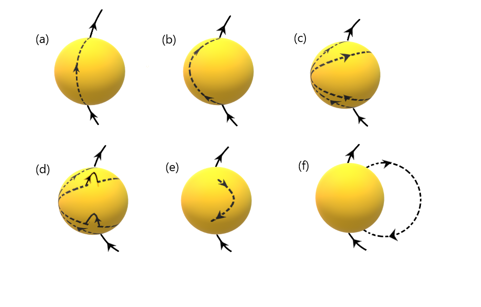
Figure 1: Pictorial representation of the Babcock–Leighton dynamo model with anti-solar DR. (a) Initial poloidal field line. (b) and (c) This field is stretched by the anti-solar DR (equator rotates slower than poles) to produce a toroidal field. (d) The toroidal field rises to the surface and form tilted BMRs with loop structures. (e) Opposite polarity of sunspots connects near the equator and create a big poloidal loop (dashed line). (f) The large-scale poloidal field developed (dashed line) is in the same orientation as that of the original one.

The most interesting feature is the change of magnetic field strength in the slowly rotating stars. As referenced above, observations of slowly rotating stars show an increase of magnetic activity with the increase of rotation period which is possibly caused by the transition of DR to anti-solar from the solar-like profile as proposed by Brandenburg & Giampapa (2018). Indeed, Karak et al. (2015) found an increase of the magnetic field in the anti-solar DR regime. Simulations of Warnecke (2018) in different parameter regimes seem to show a little increase of the magnetic field, in contrast, Viviani et al. (2018) did not find significant increase. This remains a curiosity in the community whether the magnetic field indeed increases in the anti-solar DR regime and if so, then whether this is actually caused by the anti-solar DR. The answers to these are not obvious because the strength of the dynamo, as determined by the $\alpha$ and shear, do not necessarily increase in the anti-solar DR regime (slowly rotating stars). In fact, we expect the strength of $\alpha$ to decrease with the decrease of rotation rate. Well, in simulations it has been observed that the shear is much strong in the anti-solar DR regime (see Table 1 of Karak et al. (2015) and Viviani et al. (2018)). But this cannot be the reason for the increased magnetic activity in slowly rotating stars because otherwise both Viviani et al. (2018) and Warnecke (2018) would also find an abrupt increase of magnetic field. Therefore, we shall understand the behaviour of the stellar dynamo with anti-solar DR which is found in the slowly rotating stars. We shall explore whether the increase of magnetic field as seen in observation is possible in the dynamo model with anti-solar DR and what causes this increase.

In our study, without going through the complexity of the global MHD convection simulations and saving the computational resources, we shall develop a simple kinematic dynamo model by specifying $\alpha$ and $\Omega$ for the sources of magnetic fields and make some clean simulations to explore the physics behind the magnetic cycles and polarity reversal in stars. We shall explore how the magnetic field strength varies when the DR profile changes from solar to anti-solar. We shall also present how other features of magnetic cycles, namely cycle period and the ratio of poloidal to toroidal fields change with the stellar rotation.

2 Model

In our study, we develop a kinematic mean-field dynamo model by considering only the diagonal terms of the $\alpha$ coefficients and an isotropic turbulent diffusion $\eta$. We further assume magnetic field to be axisymmetric, thus writing magnetic field $\bm{B}=\bm{\nabla}\times[A(r,\theta,t)\bm{\hat{\phi}}]+B(r,\theta,t)\bm{\hat{\phi}}$, where $A$ is vector potential for poloidal field $\bm{B_{p}}\equiv(B_{r}\bm{\hat{r}},B_{\theta}\bm{\hat{\theta}})$, $B$ is toroidal field, and $\theta$ is co-latitude. Subsequently, the equations for $A$ and $B$ can be derived as

$$\frac{\partial A}{\partial t}+\frac{1}{s}({\bm{v}_{p}}\cdot\bm{\nabla})(sA)=\eta\left(\nabla^{2}-\frac{1}{s^{2}}\right)A+\alpha_{\phi\phi}B$$ (1)

$$\frac{\partial B}{\partial t}+\frac{1}{r}\left[\frac{\partial}{\partial r}(rv_{r}B)+\frac{\partial}{\partial\theta}(v_{\theta}B)\right]=\eta\left(\nabla^{2}-\frac{1}{s^{2}}\right)B$$

$$+s(\bm{B}_{p}\cdot{\bm{\nabla}})\Omega+S^{\rm Tor}_{\alpha}(r,\theta)+\frac{1}{r}\frac{d\eta}{dr}\frac{\partial{(rB)}}{\partial{r}}$$ (2)

where $s=r\sin\theta,{\bm{v}_{p}}\equiv(v_{r}\bm{\hat{r}},v_{\theta}\bm{\hat{\theta}}))$, and

$$S^{\rm Tor}_{\alpha}(r,\theta)=-\alpha_{\theta\theta}\left(\frac{2}{r}\frac{\partial A}{\partial r}+\frac{\partial^{2}A}{\partial r^{2}}\right)$$

$$+\frac{\alpha_{rr}}{r^{2}}\left(\frac{A}{\sin^{2}\theta}-\cot\theta\frac{\partial A}{\partial\theta}-\frac{\partial^{2}A}{\partial\theta^{2}}\right)$$

$$-\frac{1}{r}\frac{\partial\alpha_{rr}}{\partial\theta}\left(\frac{A\cot\theta}{r}+\frac{1}{r}\frac{\partial A}{\partial\theta}\right)-\frac{\partial\alpha_{\theta\theta}}{\partial r}\left(\frac{A}{r}+\frac{\partial A}{\partial r}\right)$$ (3)

with $\alpha_{rr},\alpha_{\theta\theta}$ and $\alpha_{\phi\phi}$ being the diagonal components of $\alpha$ tensor. In our model, we shall ignore the off-diagonal components (which are responsible for magnetic pumping) because of the limited knowledge of their profiles in the solar and stellar convection zones (CZs) and to keep our model and the interpretation of the results tractable.

Numerical simulations of magneto-convection in local Cartesian domain (e.g., Käpylä & Brandenburg, 2009; Karak et al., 2014b) and global solar/stellar CZs (e.g., Simard et al., 2013, 2016; Warnecke et al., 2018) provide some guidance, although the simulation carried out are still far from the real Sun (in terms of its fundamental parameters). These simulations show that the $\alpha$ components are highly inhomogeneous across radius and latitudes. They change sign at the equator and have no resemblance with each other. We also note that there is some amount of uncertainty in the measurement of $\alpha$ coefficients, and so far, we do not have a well-tested method for their measurement. Thus keeping general features of the $\alpha$ coefficients as obtained through theory and simulations, we begin with the following simple profiles for $\alpha_{rr}$ and $\alpha_{\theta\theta}$.

$$\alpha_{rr}=\alpha_{0}\frac{1}{2}\left[1+\mathrm{erf}\left(\frac{r-0.7R_{s}}{0.01R_{s}}\right)\right]\cos\theta,$$ (4)

$$\alpha_{\theta\theta}=\alpha_{rr},$$ (5)

where $R_{s}$ is the solar radius; see Figure 2 top panels for the variations of this profile.

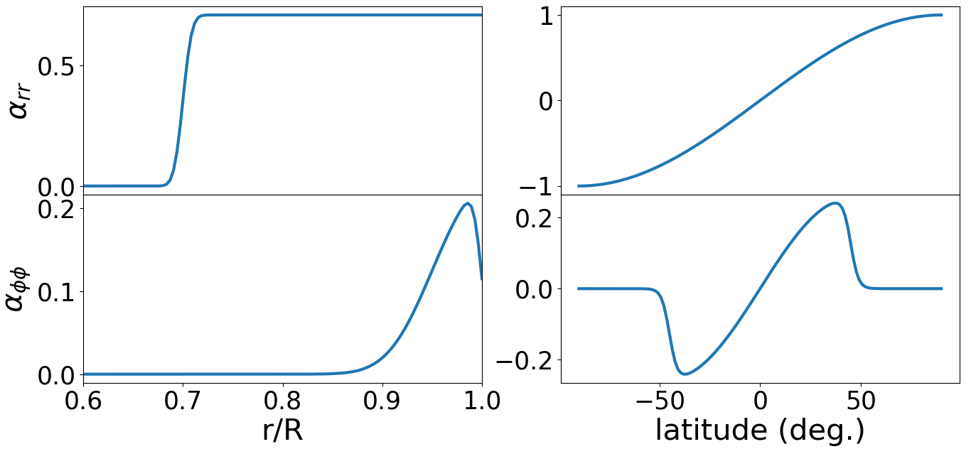
Figure 2: Left: Radial variations of $\alpha_{rr}$ (Equation (4)) and $\alpha_{\phi\phi}$ (Equation (6)) at $45^{\circ}$ latitude for $\alpha_{0}=1$ m s^-1. Right: Latitudinal variations of the same at $r=0.95R_{s}$.

For $\alpha_{\phi\phi}$, we use a different profile (Figure 2 bottom panels) and it is given by

$$\alpha_{\phi\phi}=\alpha_{0}\frac{1}{4}\left[1+\mathrm{erf}\left(\frac{r-0.95R_{s}}{0.05R_{s}}\right)\right]\left[1-\mathrm{erf}\left(\frac{r-R_{s}}{0.01R_{s}}\right)\right]$$

$$\times f_{\rm{s}}\cos\theta\sin\theta,~{}~{}~{}~{}~{}~{}~{}~{}~{}~{}~{}~{}$$ (6)

where $f_{\rm{s}}$ is a function that takes care of suppressing $\alpha_{\phi\phi}$ above $\pm 45^{\circ}$ latitudes and thus $f_{\rm{s}}=1/[1+\exp\{30(\pi/4-\theta)\}]$ for $\theta<\pi/2$ and $1/[1+\exp\{30(\theta-3\pi/4)\}]$ for otherwise. We take this factor $f_{\rm{s}}$ in $\alpha_{\phi\phi}$ to restrict the strong toroidal field and thus the band of formation of sunspots in the low latitudes, which is a common practice in the flux transport dynamo models (Küker et al., 2001; Dikpati et al., 2004; Guerrero & de Gouveia Dal Pino, 2007; Hotta & Yokoyama, 2010; Karak & Cameron, 2016). Further, we choose $\alpha_{\phi\phi}$ to operate only near the surface so that the source for the poloidal field is slightly segregated from the source for the toroidal field. This, in turn, helps in producing longer cycle period of 11 years. For $\alpha_{rr}$ and $\alpha_{\theta\theta}$ we keep the profiles simple so that they both are non-zero in the whole CZ and have a $\cos\theta$ dependence. Later in §4, we shall also use different $\alpha$ profiles and explore the robustness of our results.

To limit the growth of magnetic field in our kinematic dynamo model, we consider following simple nonlinear quenching

$$\alpha_{ii}=\frac{\alpha_{ii}}{1+\left(\frac{B}{B_{0}}\right)^{2}}$$ (7)

where $i=r,\theta,\phi$ and $B_{0}$ is the saturation field strength which is fixed at $4\times 10^{4}$ G in all the simulations. Because of this nonlinear saturation, we always present the magnetic field from our model with respect to $B_{0}$.

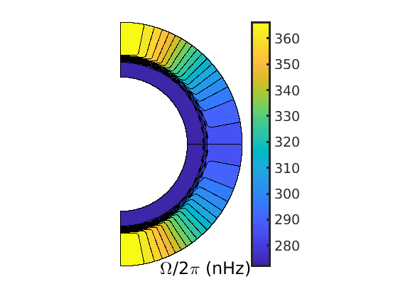
Figure 3: Angular frequency $\Omega/2\pi$ for the anti-solar DR; see Equation (8).

For DR, we take following profile which reasonably fits the helioseismology data

$$\Omega(r,\theta)=\Omega_{\mathrm{RZ}}+\frac{1}{2}\left[1+\mathrm{erf}\left(\frac{r-0.7R_{s}}{0.025R_{s}}\right)\right]\left(\Omega_{\mathrm{CZ}}-\Omega_{\mathrm{RZ}}\right),$$ (8)

where $\Omega_{\mathrm{RZ}}/2\pi=432.8$ nHz, and $\Omega_{\mathrm{CZ}}/2\pi=460.7-62.69\cos^{2}\theta-67.13\cos^{4}\theta$ nHz. When we make the DR anti-solar, we take $\Omega_{\mathrm{CZ}}/2\pi=460.7+62.69\cos^{2}\theta+67.13\cos^{4}\theta$ nHz. Note that this will allow $\Omega$ to increase with latitudes and that is the anti-solar DR which is shown in Figure 3.

The turbulent magnetic diffusivity $\eta$ has the following form:

$$\eta(r)=\eta_{\mathrm{RZ}}+\frac{\eta_{\mathrm{SCZ}}}{2}\left[1+\mathrm{erf}\left(\frac{r-0.7R_{s}}{0.02R_{s}}\right)\right]+\frac{\eta_{\mathrm{surf}}}{2}\left[1+\mathrm{erf}\left(\frac{r-0.9R_{s}}{0.02R_{s}}\right)\right],$$ (9)

where $\eta_{\mathrm{RZ}}=5\times 10^{8}$ cm² s^-1, $\eta_{\mathrm{SCZ}}=5\times 10^{10}$ cm² s^-1, and $\eta_{\mathrm{surf}}=2\times 10^{12}$ cm² s^-1. Meridional circulation ($v_{r}$ and $v_{\theta}$) profile is the same as given in Hotta & Yokoyama (2010); also see Dikpati et al. (2004); Karak et al. (2014a); Karak & Petrovay (2013). For the sake of completeness, we write these profiles and boundary conditions in Appendix A.

3 Results

We start all simulations by specifying some initial magnetic field, and we analyse the results only after running the code for several diffusion times so that the magnetic field reaches a statistically stationary state. We first present the result of an $\alpha^{2}$ model by setting $\Omega=0$. As the results for such a dynamo model for the Sun with parameters given above has not been presented before, we shall first show the result.

3.1 Solar dynamo without differential rotation

The critical $\alpha_{0}$ for the $\alpha^{2}$ dynamo model without DR for the Sun is about $10$ m s^-1. However, the prominent dynamo cycles with polarity reversals are seen only when $\alpha_{0}$ is approximately above 18 m s^-1. Butterfly diagram for $\alpha_{0}=20$ m s^-1 is shown in Figure 4. We notice that even this model without DR produces some basic features of the solar cycle, namely, (i) the polarity reversal, (ii) 11-year periodicity, (iii) equatorward migration of toroidal field at the base of the CZ, and (iv) the poleward migration of surface poloidal field. Feature (i) is due to the selected inhomogeneous profile of $\alpha$ taken in our model. The other properties are largely determined by the inclusion of meridional flow which is poleward near the surface and equatorward near the base of the CZ and a relatively weak diffusivity in the bulk of the CZ.

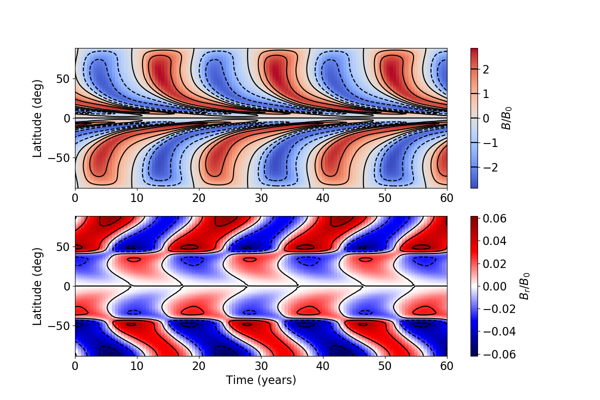
Figure 4: Result of $\alpha^{2}$ dynamo model with meridional circulation. Time-latitude diagrams of (a) toroidal magnetic field $B$ at $r=0.7R_{s}$ and surface radial field $B_{r}$. All fields are measured with respect to $B_{0}$.

The oscillatory magnetic field in $\alpha^{2}$ dynamo in spherical geometry is not new. It was realized that the $\alpha^{2}$ dynamo with certain $\alpha$ profiles (Baryshnikova & Shukurov, 1987; Stefani & Gerbeth, 2003; Elstner & Rüdiger, 2007), and/or boundary conditions (Mitra et al., 2010; Jabbari et al., 2017) produces an oscillatory solution. We also note that the mean-field model constructed using $\alpha$ profiles obtained from the global MHD simulation also finds oscillatory solution (Simard et al., 2013).

3.2 Stellar dynamo with solar and anti-solar DR

Now we perform dynamo simulations of different stars with rotation period 1, 5, 10, 17, 25.38 (solar value), 30, 32, 40 and 50 days. As discussed in the introduction that the slowly rotating stars are expected to have anti-solar DR, which is, at least, confirmed in the global MHD simulations. This transition from solar to anti-solar DR is possibly happening below the solar rotation with Rossby number not too far from unity. Therefore, we assume that all stars with rotation periods up to 30 days are having solar-like DR, while stars of periods longer than 30 days have anti-solar DR. Further, the amount of internal DR is expected to change with the rotation rate. Hence, we choose it to scale in the following way.

$$\Omega(r,\theta)=\left(\frac{T_{s}}{T}\right)^{n}\Omega_{s}(r,\theta),$$ (10)

where $T_{s}=25.38$ days (solar rotation period), $T$ is the rotation period of star, and $\Omega_{s}(r,\theta)$ is the internal angular frequency of the Sun as given in Equation (8). Some numerical simulations suggest $n$ is about 0.3 (Ballot et al., 2007; Brown et al., 2008), while the recent work of Viviani et al. (2018) in a more wider range finds $n\approx-0.08$ for the rotation rates up to 5 times solar value and $n=-0.96$ for rotation rate of 5–31 times the solar rotation. Surface observations find somewhat similar results, for example, Barnes et al. (2005), Reinhold & Gizon (2015), Donahue et al. (1996), and Lehtinen et al. (2016) respectively give $n=0.15,0.29,0.7,$ and $-0.36$. In our study, we perform two sets of simulations by considering two values, namely $n=0.7$, i.e., the DR increases with the increase of rotation rate with an exponent of $0.7$ and $n=0.0$, i.e. no change in DR. These two sets of simulations are labelled as A1–A50 and B1–B50; see Table 1.

Table 1: Summary of simulations. Here, $T$ is the rotation period of star in days, $P_{\rm cyc}$ is the mean magnetic cycle period, SL and AS stand for solar and anti-solar DR, respectively.

Details	Run	$T$ (d)	DR	$\frac{B_{\rm tor}}{B_{0}}$	$\frac{B_{\rm pol}}{B_{0}}$	$P_{\rm cyc}$ (yr)
Set A:	A1	1	SL	6.346	0.329	….
$\Omega$ and $\alpha$	A5	5	SL	1.636	0.066	….
change	A10	10	SL	0.663	0.051	3.30
following	A17	17	SL	0.361	0.035	2.00
Eqs.	A25	25.38	SL	0.141	0.028	7.41
10–11.	A30	30	SL	0.128	0.024	7.60
	A32	32	AS	0.582	0.081	22.95
	A40	40	AS	0.623	0.066	20.95
	A50	50	AS	0.575	0.053	18.52
Set B:	B1	1	SL	5.885	0.340	….
Same as	B5	5	SL	1.702	0.071	2.10
Set A but	B10	10	SL	0.355	0.053	3.40
no change	B17	17	SL	0.326	0.037	7.92
in DR.	B25	25.38	SL	0.140	0.023	7.38
	B30	30	SL	0.213	0.023	7.20
	B32	32	AS	0.680	0.081	24.31
	B40	40	AS	0.748	0.066	21.13
	B50	50	AS	0.708	0.054	19.41
Set C:	C1	1	SL	3.628	0.146	….
Same as	C5	5	SL	1.534	0.057	2.54
Set A but	C10	10	SL	0.370	0.048	6.53
meridional	C17	17	SL	0.399	0.036	2.82
flow	C25	25.38	SL	0.141	0.028	7.41
changes	C30	30	SL	0.062	0.010	7.51
following	C32	32	AS	0.603	0.082	19.96
Eqs. 12	C40	40	AS	0.701	0.070	15.52
	C50	50	AS	0.251	0.024	12.19
Set D:	D1	1	SL	0.762	0.0319	10.50
Same as	D5	5	SL	0.287	0.0051	9.206
Set A but	D10	10	SL	0.261	0.0054	12.49
$\alpha_{rr}$, $\alpha_{\theta\theta}$	D17	17	SL	0.186	0.0041	12.33
are taken	D25	25.38	SL	0.133	0.0030	12.33
from Eqs.	D30	30	SL	0.110	0.0025	12.24
13–14	D32	32	AS	0.119	0.0032	14.09
	D40	40	AS	0.115	0.0033	14.23
	D50	50	AS	0.110	0.0035	14.22
Set E:	E1	1	SL	4.578	1.956	….
Same as	E5	5	SL	1.999	0.8728	0.54
Set A but	E10	10	SL	1.266	0.5821	1.86
all $\alpha$ are	E17	17	SL	1.113	0.4765	2.23
taken from	E25	25.38	SL	0.573	0.293	2.92
Eq. 15	E30	30	SL	0.445	0.250	2.95
and high	E32	32	AS	0.450	0.355	7.93
diffusivity.	E40	40	AS	0.300	0.313	4.90
	E50	50	AS	0.233	0.272	4.83

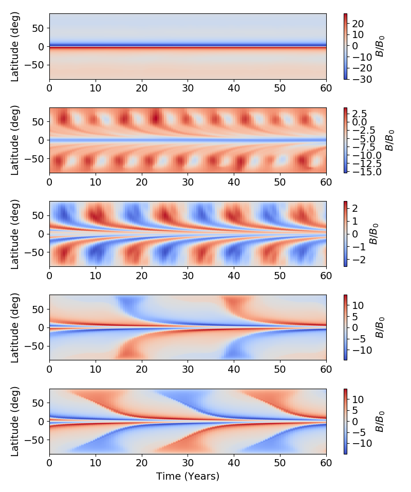
Figure 5: Butterfly diagram of the toroidal field averaged over a thickness of $0.04R_{s}$ centered at $0.71R_{s}$ from stars of rotation periods 5, 10, 25.38 (Sun), 32, and 50 days (top to bottom); Runs A5, A10, A25, A32, and A50.

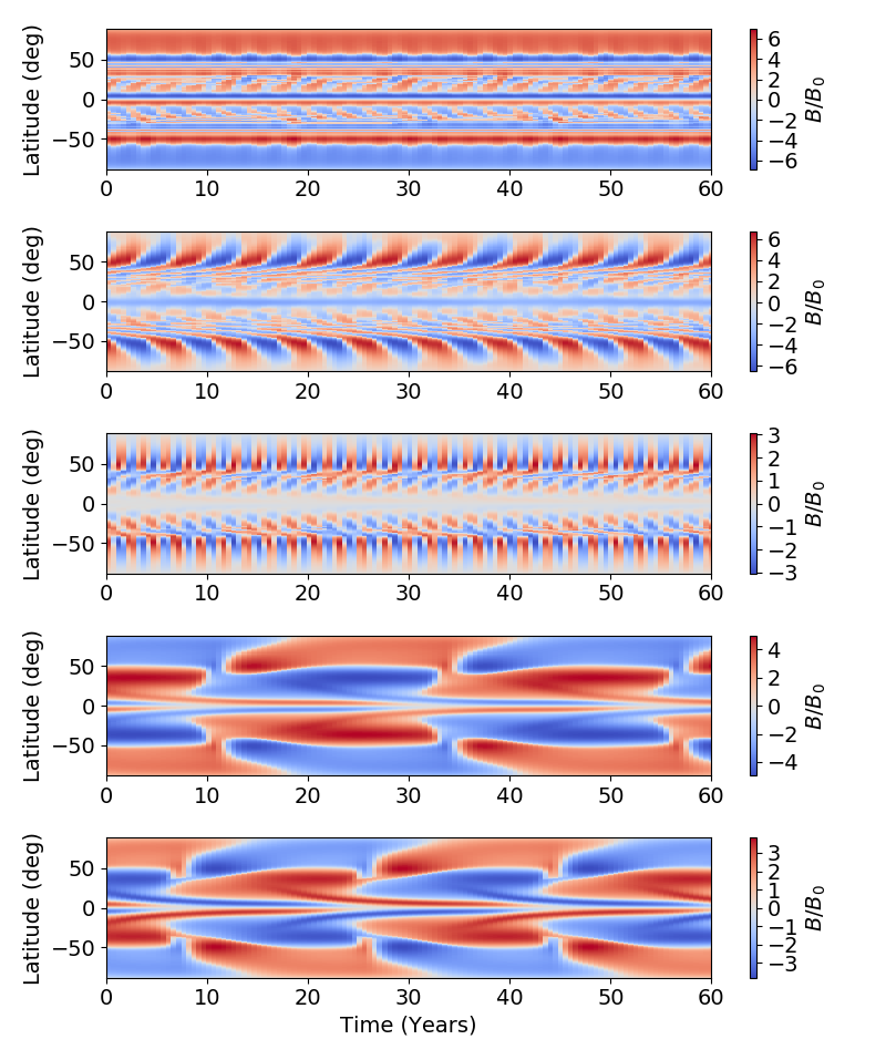
Figure 6: Same as Figure 5 but obtained from the toroidal field at $0.85R_{s}$.

Figure 7: Top–bottom: Dependences of the magnetic field, the ratio of toroidal to poloidal fields, and cycle periods with rotation periods of the stars. Circular and asterisk points are obtained from simulations in which DR decreases with rotation period through Equation (10) (Runs A1–A50) and DR does not change (Runs B1–B50), respectively. Triangular points come from the same simulations as that of circular points but the meridional circulation is increased with rotation period through Equation (12) (Runs C1–C50). The shaded area represents the solar-like DR regime, while the white space is anti-solar.

The amplitude of $\alpha$ is also expected to increase with the increase of rotation rate (Krause & Rädler, 1980). As we do not know how exactly $\alpha$ scales with the rotation rate, we choose it to increase linearly. Thus, in Equations (4–6), we take

$$\alpha_{0}=\frac{T_{s}}{T}\alpha_{0,s},$$ (11)

where $\alpha_{0,s}$ is the value of $\alpha_{0}$ for the solar case, in which we take $\alpha_{0,s}=80$ m s^-1.

The meridional circulation is another important ingredient in the model which is expected to vary with the rotation rate. Our knowledge of meridional circulation even for the sun is very limited. Mean-field models and global convection simulations all suggest that its profile as well as amplitude changes with the rotation rate (Kitchatinov & Olemskoy, 2011b; Featherstone & Miesch, 2015; Karak et al., 2015; Karak et al., 2018a). Simulations of Brown et al. (2008) showed that the kinetic energy of meridional circulation approximately scales as $\Omega^{-0.9}$. Therefore in one set of simulations (Runs C1–C50 in Table 1), we shall change meridional circulation along with other parameters in the following way.

$$v_{0}=\left(\frac{T_{s}}{T}\right)^{-0.45}v_{0,s},$$ (12)

where $v_{0,s}$ is the amplitude of meridional circulation of sun, for which we have taken 10 m s^-1. We do not make any other changes in the model.

Interestingly, all the stars, including ones with anti-solar DR (rotation periods 32–50 days), show prominent dynamo cycles and polarity reversals except for the very rapidly rotating star of rotation period 1 day. The butterfly diagrams of stars with rotation periods 5, 10, 25.38, 32, and 50 days (from Runs A1–A50) are shown in Figures 5 and 6. We observe that the 5 days rotating star (Run A5) does not show magnetic cycle at the base of the CZ, but it does some cycles in low latitudes of mid-CZ. The magnetic fields are largely anti-symmetric across the equator in all the cases. The equatorward migration is largely due to the return meridional flow.

To quantify how the magnetic field strength and cycle period change with different stars, we compute the root-mean-square ($rms$) field strength $B_{rms}=\sqrt{\left\langle(B_{r}^{2}+B_{\theta}^{2}+B_{\phi}^{2})\right\rangle}$, the ratio of poloidal to toroidal field Bpol/Btor $=\sqrt{\left\langle(B_{r}^{2}+B_{\theta}^{2})\right\rangle}/\sqrt{\left\langle B_{\phi}^{2}\right\rangle}$ (where angular brackets denote the average over the whole domain), and the mean period of the polarity reversals of the toroidal field. These quantities are listed in Table 1 and the variations with rotation period are shown in Figure 7.

In the rapidly rotating regime, the magnetic field strength increases with the decrease of rotation period, which is in agreement with observations (Petit et al., 2008). This behaviour in fact is not very surprising because the magnetic field sources ($\alpha$ and $\Omega$) are increased with the rotation rates through equations (11) and (10). However, what is surprising in Figure 7(a) is that the magnetic field abruptly increased just above the rotation period of 30 days. That is the point where the DR pattern is changed from solar-like to anti-solar. Thus the anti-solar DR causes a sudden increase of magnetic field in the slowly rotating stars, which is in good agreement with the stellar observational data (Giampapa et al., 2006, 2017; Brandenburg & Giampapa, 2018) and also with global MHD convection simulations (Karak et al., 2015). Further, we note that even the simulations (Run B1–B50; red asterisks in Figure 7a) in which $\Omega$ does not change with the rotation rate (i.e., $n=0$ in Equation (10)) also produces a similar variation of magnetic field. As the shear is not decreased in this case, the field in the anti-solar branch is little stronger in comparison to Set A (black points). The Set C, in which meridional flow is increased with the rotation period (Equation (12)), also show a similar variation of magnetic field (blue triangles in Figure 7a), which is unusual in the $\alpha\Omega$ type flux transport dynamo models (Karak, 2010).

To understand the enhancement of the magnetic field in the anti-solar DR regime, we perform the following experiment. We consider the simulation of the 30-day rotation period having solar-like DR (Run A30). We first make sure that this model is producing a steady dynamo solution. Then, when the toroidal field reverses, that is when the toroidal field is at a minimum, we stop the code. The vertical line at $t=10$ years in Figure 8 shows this time. Then we make the DR anti-solar and run the code for four years (up to the second vertical line in Figure 8). Finally, we revert the DR to the solar-like profile and continue the run for another 10 years. We see a significant increase of magnetic field in Figure 8(a) after the DR is made anti-solar. This increase of field must be caused by the change in DR from solar to anti-solar profile. We know that during the reversal, the anti-solar DR produces toroidal field of the same sign as that of the previous cycle. As seen in Figure 8(a), when the toroidal field in the northern hemisphere is mostly negative during the phase of anti-solar DR ($t=$10–14 years), the dynamo needs a positive field to reverse it. However, the anti-solar DR gives negative polarity field, and thus, it tries to enhance the old field (negative in the northern hemisphere). So essentially what is happening is the following:
Pol($+$)  $\overrightarrow{(Solar~{}\Omega)}$  Tor($-$)  $\overrightarrow{\alpha}$  Pol($-$)  $\overrightarrow{(Anti{-}sol~{}\Omega)}$  Tor($-$).
Note in the last phase, the toroidal field is produced in the same polarity as that of the previous cycle and thus the field is enhanced; also see Figure 1. We may mention that instead of anti-solar DR if the $\alpha$ is reversed, then also the same effect will be seen. In fact, following this idea, recently Karak et al. (2018b) explained the sudden increase of the poloidal field and appearance of double peaks in the sunspot cycles using a momentarily reversed $\alpha$ due to wrong BMR tilt.

Later, when the DR is changed to solar-like, this increasing effect of anti-solar DR is stopped and the model succeed to reverse the field (at around $t=16$ years in Figure 8). We note that the increase of magnetic field is not immediately seen in the averaged field at the base of the CZ in Figure 8(b) because of the cancellation and finite transport time, but it is clearly seen in the next cycle.

Figure 8: Simulation result of a star with rotation period 30 days in which the DR is made anti-solar during 10–14 years (identified by two vertical lines). Butterfly diagram of (a) the toroidal field at $0.85R_{s}$ and (b) the same but averaged over a thickness of $0.04R_{s}$ centered at $0.71R_{s}$.

Above discussion shows that the anti-solar DR amplifies the old toroidal field by supplying toroidal field of the same polarity. Thus we do not expect polarity reversal if the anti-solar DR acts for all the time and if there is no other source for the toroidal field generation. In our model, we certainly have $\alpha$ effect for the generation of the toroidal field in addition to $\Omega$. However, this may not be sufficient to reverse the field. We realized that when the toroidal field has reached a very high value, the DR is needed to be suppressed otherwise the $\alpha$ effect is not able to reverse the toroidal field and the cyclic dynamo is not possible. When the toroidal field is sufficiently high due to anti-solar DR, it is expected that this strong field acts back on the DR through Lorentz forces and tries to suppress the shear. The suppression mechanism could be complicated as the strong magnetic field can give Lorentz forces on the large-scale flows as well as suppress the convective angular momentum transport (see e.g, Karak et al., 2015; Käpylä et al., 2016). The bottom line is that the shear must be decreased once the toroidal field reaches a sufficiently high value. This, in fact, is seen in the simulations of Karak et al. (2015) that the shear parameters are quenched when the magnetic field is strong; see their Fig. 13(e-f). We also note that even in the Sun, there is an indication of the reduction of shear during the solar maximum; see Fig. 6–7 of Antia et al. (2008) and also Barekat et al. (2016). Motivated by these, we have introduced a nonlinear magnetic field dependent quenching $f_{q}=1/\left(1+(B/B_{0})^{2}\right)$ in the shear such that $\bm{\nabla}\Omega$ in Equation (2) is replaced by $f_{q}\bm{\nabla}\Omega$. Through this nonlinear quenching, the toroidal field tries to reduce the shear when it exceeds $B_{0}$. In Figure 9(b), we observe that the shear is strong during cycle minimum and thus, it produces a strong toroidal field. Then the strong field quenches the shear and the toroidal field cannot grow rapidly. Interestingly, the toroidal field generation due to $\alpha$ effect $S^{\rm Tor}_{\alpha}$ (see Equation (3)) is not negligible (Figure 9(c)) and it is this process which eventually dominates and reverses the toroidal field slowly. Essentially, it is the nonlinear competition between the toroidal field generation through shear and $\alpha$, which makes the polarity reversal possible even with the anti-solar DR.

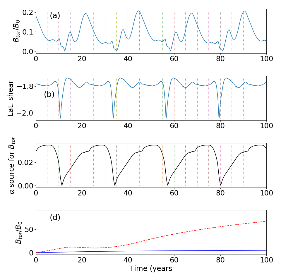
Figure 9: Results from Run A32 computed over the whole CZ in the northern hemisphere: Temporal variations of (a) the toroidal field, (b) the mean effective latitudinal shear $\frac{1}{r}\frac{\partial\Omega}{\partial\theta}/\left(1+(B/B_{0})^{2}\right)$ (in unit of $10^{-9}$ nHz deg^-1), (c) the mean source term due to $\alpha$ effect for the toroidal field ($S^{\rm Tor}_{\alpha}$ in Equation (2) in unit of $10^{-6}$s^-1), and (d) the same as (a), but obtained from simulations in which there is no quenching in the shear (red dashed line) and $\alpha_{0}=20$ m s^-1 (solid blue), instead of 80 m s^-1 which is used in all Runs A1–A50.

To further support above conclusion, we show that if we do not include the quenching (i.e., $f_{q}=1$) in the shear, then the dynamo fails to reverse the magnetic field, rather the toroidal field increases in time; see red/dashed line in Figure 9(d). On the other hand, if we keep the quenching in shear but reduce the strength of $\alpha$ by $75\%$, then also, dynamo fails to reverse the cycle and the magnetic field remains steady; see blue/solid line in Figure 9(d). In conclusion, to obtain the polarity reversal with anti-solar DR, there must be a sufficiently strong $\alpha$ and the shear must be reduced when the toroidal field becomes very strong.

Returning to Figure 7(b), we observe that for all the stars, the mean poloidal field is about one order of magnitude smaller than that of the toroidal field. The ratio Bpol/Btor has a non-monotonous behaviour. It is maximum at the solar rotation and decreases on both sides. This implies that the toroidal field dominates over the poloidal field both for rapidly and slowly rotating stars. With the increase of rotation rate, the toroidal field must increase faster than the poloidal component because there are two sources of toroidal field ($\alpha$ and shear) and both increase with the rotation rate. In the anti-solar branch, Bpol/Btor decreases because toroidal field generation is stronger with the anti-solar DR. The increase of poloidal contribution with the increase of cycle period in the solar-like DR branch is in agreement with the observational findings (Petit et al., 2008). These observational results also show that the magnetic energy of the toroidal field dominates below the rotation period of 12 days, while in our simulations the toroidal energy is always greater than the poloidal field. We should not forget that observational results are based on the field what was detected and it could be that most of the toroidal field in observations was not be detected. Therefore, instead of comparing the actual value of magnetic energy, we should see how the ratio of poloidal to toroidal field changes with the rotation rate and this is in somewhat agreement with observation (compare Figure 6 of Petit et al. (2008) with the left branch of our Figure 7(b)). Unfortunately, Petit et al. (2008) do not have data in the slowly rotating branch above the solar rotation period and thus we cannot compare this behaviour with observations.

Finally, the cycle period again shows a non-monotonous behaviour. It decreases with the increase of rotation rate, which is in general agreement with observations (Noyes et al., 1984b; Suárez Mascareño et al., 2016; Boro Saikia et al., 2018), although the observational trend is messy. The slow decrease of rotation period in the anti-solar DR branch is not apparent in the observed data; see, for example, Fig. 9 of Boro Saikia et al. (2018). In our model, the decrease of cycle period with the increase of rotation rate is because the dynamo becomes stronger with the rotation rate which makes the conversion between poloidal and toroidal faster and reduces the cycle period. In global MHD simulations of stellar dynamos, Guerrero et al. (2018) also find a decrease of period with the increase of rotation rate, while Warnecke (2018) find this trend only at slow rotation and then an increasing trend in the rapid rotation. In latter simulations, the increase of period with rotation rate is due to the decrease of shear. In our study, when the DR is anti-solar, it tries to produce the same polarity field as that of the previous cycle and thus $\alpha$ takes longer time to reverse the field—causing the cycle longer. This effect decreases when the rotation period is too long because the strength of the anti-solar DR decreases and thus the polarity reversal becomes faster. This causes the cycle period to shorten with the increase of rotation period in the anti-solar branch.

As the meridional flow transports the magnetic fields from source regions, the cycle duration tends to be longer with the decrease of meridional flow (Dikpati & Charbonneau, 1999; Karak, 2010). This was usually seen in previous flux transport dynamo models of stellar cycles (Nandy, 2004; Jouve et al., 2010; Karak et al., 2014a), but not in the turbulent pumping-dominated regime (Karak & Cameron, 2016; Hazra et al., 2019). Therefore, in Set C in which meridional circulation is decreased with the rotation rate following Equation (12), we expected an increase of cycle period. However, we see a reverse trend (see blue points in Figure 7(c)), because the dynamo becomes stronger and this tries to make the cycle shorter.

4 Robustness of our results

We have above seen that the results are only little sensitive to the change in $\Omega$ and meridional circulation. Notably, the enhancement of the magnetic field at the transition point from solar to anti-solar DR is prominent. To explore the robustness of these results further, we consider different profiles for $\alpha$. In principle, we can consider countless different profiles for $\alpha$ as the actual profiles are not known even for the Sun. Different profiles will make the dynamo solutions different but not necessarily the variations of magnetic field with rotation period. To demonstrate this, we present the results for two more sets of simulations, namely, Set D (Runs D1–D50) and set E (Runs E1–E50); see Table 1.

In Set D, we change $\alpha_{rr}$ and $\alpha_{\theta\theta}$ to as follows:

$$\alpha_{rr}=\alpha_{0}\sin\left[2\pi\left(\frac{r-0.7R_{s}}{0.3R_{s}}\right)\right]\cos\theta\sin^{2}\theta,$$ (13)

$$\alpha_{\theta\theta}=\alpha_{0}\sin\left[2\pi\left(\frac{r-0.7R_{s}}{0.3R_{s}}\right)\right]\cos\theta,$$ (14)

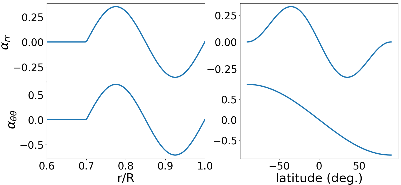
Figure 10: Left: Radial variations of $\alpha_{rr}$ and $\alpha_{\theta\theta}$ in m s^-1 at $45^{\circ}$ latitude. Right: Latitudinal variations of the same at $r=0.95R_{s}$. These are the profiles used in Set D; Equation (14) with $\alpha_{0}=1$ m s^-1.

both for $r\geq 0.7R_{s}$, while $\alpha_{rr}=\alpha_{\theta\theta}=0$ for $r<0.7R_{s}$ and $\alpha_{0}=100$ m s^-1; see Figure 10 for these profiles. No other parameters are changed in this Set.

On the other hand, in Set E, we change all three $\alpha$ profiles to followings.

$$\alpha_{rr}=\alpha_{\theta\theta}=\alpha_{\phi\phi}=\alpha_{0}\frac{1}{2}\left[1+\mathrm{erf}\left(\frac{r-0.7R_{s}}{0.01R_{s}}\right)\right]\cos\theta.$$ (15)

With these new $\alpha$, we, however, do not get polarity reversal in a wide range of $\alpha_{0}$ both in solar and anti-solar DR cases. Interestingly, this new $\alpha$ profile gives polarity reversals if we increase the diffusivity in the bulk of the CZ. That is, when we take $\eta_{\mathrm{SCZ}}=1\times 10^{12}$ cm² s^-1, $\eta_{\mathrm{surf}}=1.05\times 10^{12}$ cm² s^-1(see Figure 11 dashed line) and $\alpha_{0}=80$ m s^-1, we obtain polarity reversals in all runs except Run E1; see Figure 12. It could be that in this new $\alpha$ profile, unless we increase the diffusion in the deeper CZ, the toroidal field generation due to shear overpowers the same due to $\alpha$ effect. This higher diffusion makes the equatorward migration of toroidal field less important and the magnetic field in run E50 quadrupolar.

We note that with these new $\alpha$ profiles, we again obtain a clear increase of magnetic field in both the sets D and E; see Table 1, although the increase is relatively small. We note that in both sets, $\alpha$ and $\Omega$ are decreased with the increase of rotation period as before following equations (11) and (10).

5 Conclusion

In this study, using a mean-field kinematic dynamo model we have explored the features of large-scale magnetic fields of solar-like stars rotating at different rotation periods and having the same internal structures as that of the Sun. Our main motivation is to understand the large-scale magnetic field generation in the slowly rotating stars with rotation period larger than the solar value. This region is of particular interest because these stars possibly possess anti-solar DR and thus the operation of dynamo can be fundamentally different than stars having the usual solar-like DR.

By carrying out simulations for different stars at different model parameters, we show that the fundamental features of stellar magnetic field change with rotation period. In the solar-like DR branch, we find the magnetic field strength increases with the decrease of rotation period. This result is, in general, agreement with the observational findings (Noyes et al., 1984a; Petit et al., 2008; Wright et al., 2011; Wright & Drake, 2016), the global MHD convection simulations (Viviani et al., 2018; Warnecke, 2018), and mean-field dynamo modellings (Jouve et al., 2010; Karak et al., 2014a; Kitchatinov & Olemskoy, 2015; Hazra et al., 2019). However, our model does not produce the observed saturation of magnetic field in the very rapidly rotating stars, which in the kinematic models, requires some additional dynamo saturation (Karak et al., 2014a; Kitchatinov & Olemskoy, 2015). In the slowly rotating stars, we see a sudden jump of magnetic field strength at the point where the DR profile changes to anti-solar from solar. This result is in agreement with the stellar observations (Giampapa et al., 2006, 2017; Brandenburg & Giampapa, 2018) and also with the MHD convection simulations of Karak et al. (2015) and Warnecke (2018). The abrupt increase of magnetic field is due to the anti-solar DR which amplifies the existing toroidal field by supplying the same polarity field. The idea of the enhancement of magnetic field due to the change of DR was already proposed by Brandenburg & Giampapa (2018), however, no detailed dynamo modelling was performed.

We further show that with particular $\alpha$ profiles, the polarity reversal of the large-scale magnetic field is possible even in the slowly rotating stars with anti-solar DR rotation provided, (i) there is a sufficiently strong $\alpha$ for the generation of toroidal field and (ii) the anti-solar DR is non-linearly modulated with the magnetic field such that when the toroidal field becomes strong, it quenches the shear. Our conclusion of polarity reversal in general supports the work of Viviani et al. (2019), who showed that the polarity in their global MHD convection with anti-solar DR is possible as the magnetic field generation through $\alpha$ effect is comparable to that of $\Omega$ effect.

One may argue that the global MHD convection simulations of stellar CZs are still far from the real stars and there is always a question to what extent the results from these simulations hold to the real stars. Interestingly, one robust result of these simulations is that they all produce anti-solar DR in the slowly rotating stars with rotation period somewhere above the solar value with Rossby number around one. Available techniques are still insufficient to confirm the existence of anti-solar DR in solar-like dwarfs; see Reinhold & Arlt (2015). However, this has been confirmed in some K-giants (Strassmeier et al., 2003; Weber et al., 2005; Kővári et al., 2017) and subgiants (Harutyunyan et al., 2016). The enhancement of magnetic activity in the slowly rotating stars and its generation through the anti-solar DR give another support for the existence of anti-solar DR in slowly rotating dwarfs. Furthermore, this study along with previous observational results and global simulations suggest that the slowly rotating stars possess strong large-scale magnetic fields and possibly polarity reversals and cycles. These slowly rotating solar-like stars may also be prone to produce superflares (Maehara et al., 2012), which was also suggested by Katsova et al. (2018).

Appendix A Supplementary material

The meridional flow is obtained from the following analytical form.

$$v_{r}(r,\theta)=v_{0}\left(\frac{R_{s}}{r}\right)^{2}\left[\frac{-1}{m+1}+\frac{c_{1}}{2m+1}\xi^{m}-\frac{c_{2}}{2m+p+1}\xi^{m+p}\right]$$

$$\xi\left[2\cos^{2}\theta-\sin^{2}\theta\right]$$ (16)

$$v_{\theta}(r,\theta)=v_{0}\left(\frac{R_{s}}{r}\right)^{3}\left[-1+c_{1}\xi^{m}-c_{2}\xi^{m+p}\right]\sin\theta\cos\theta,$$ (17)

with

$$\xi(r)=\frac{R_{s}}{r}-1,~{}c_{1}=\frac{(2m+1)(m+p)}{(m+1)p}\xi^{-m}_{p},$$

$$c_{2}=\frac{(2m+p+1)m}{(m+1)p}\xi^{-(m+p)}_{p},~{}\mathrm{and}~{}\xi_{p}=\frac{R_{s}}{r_{p}}-1.$$ (18)

Here $m=0.5$, $p=0.25$, $v_{0}=10$ m s^-1, and $r_{p}=0.62R_{s}$. The boundary conditions are exactly taken from Chatterjee et al. (2004) and thus we do not repeat those here. For the initial magnetic field, we take

$$A=0~{}~{}~{}{\textrm{and}}~{}~{}~{}~{}~{}~{}~{}~{}~{}~{}~{}~{}~{}~{}~{}~{}~{}~{}~{}~{}~{}~{}~{}~{}~{}~{}~{}~{}$$

$$B=B_{0}\sin(2\theta)\sin\left[\frac{\pi(r-0.55R_{s})}{(R_{s}-0.55R_{s})}\right].$$ (19)

Figure 11: Solid line: diffusivity profile $\eta$ used in all the sets of simulations, except Set E for which the profile shown by the dashed line is used.

Figure 12: Same as Figure 5, but obtained from Runs E5, E17, E25, E32, E50 (top to bottom).

References

- Antia et al. (2008) Antia H. M., Basu S., Chitre S. M., 2008, ApJ, 681, 680
- Baliunas et al. (1995) Baliunas S. L., et al., 1995, ApJ, 438, 269
- Ballot et al. (2007) Ballot J., Brun A. S., Turck-Chièze S., 2007, ApJ, 669, 1190
- Barekat et al. (2016) Barekat A., Schou J., Gizon L., 2016, A&A, 595, A8
- Barnes et al. (2005) Barnes J. R., Collier Cameron A., Donati J. F., James D. J., Marsden S. C., Petit P., 2005, MNRAS, 357, L1
- Baryshnikova & Shukurov (1987) Baryshnikova I., Shukurov A., 1987, Astronomische Nachrichten, 308, 89
- Boro Saikia et al. (2018) Boro Saikia S., et al., 2018, A&A, 616, A108
- Brandenburg & Giampapa (2018) Brandenburg A., Giampapa M. S., 2018, ApJ, 855, L22
- Brown et al. (2008) Brown B. P., Browning M. K., Brun A. S., Miesch M. S., Toomre J., 2008, ApJ, 689, 1354
- Brun & Browning (2017) Brun A. S., Browning M. K., 2017, Living Reviews in Solar Physics, 14, 4
- Cameron & Schüssler (2015) Cameron R., Schüssler M., 2015, Science, 347, 1333
- Chatterjee et al. (2004) Chatterjee P., Nandy D., Choudhuri A. R., 2004, A&A, 427, 1019
- Dasi-Espuig et al. (2010) Dasi-Espuig M., Solanki S. K., Krivova N. A., Cameron R., Peñuela T., 2010, A&A, 518, A7
- Dikpati & Charbonneau (1999) Dikpati M., Charbonneau P., 1999, ApJ, 518, 508
- Dikpati et al. (2004) Dikpati M., de Toma G., Gilman P. A., Arge C. N., White O. R., 2004, ApJ, 601, 1136
- Donahue et al. (1996) Donahue R. A., Saar S. H., Baliunas S. L., 1996, ApJ, 466, 384
- Elstner & Rüdiger (2007) Elstner D., Rüdiger G., 2007, Astronomische Nachrichten, 328, 1130
- Fan & Fang (2014) Fan Y., Fang F., 2014, ApJ, 789, 35
- Featherstone & Miesch (2015) Featherstone N. A., Miesch M. S., 2015, ApJ, 804, 67
- Garg et al. (2019) Garg S., Karak B. B., Egeland R., Soon W., Baliunas S., 2019, arXiv e-prints, p. arXiv:1909.12148
- Gastine et al. (2014) Gastine T., Yadav R. K., Morin J., Reiners A., Wicht J., 2014, MNRAS, 438, L76
- Giampapa et al. (2006) Giampapa M. S., Hall J. C., Radick R. R., Baliunas S. L., 2006, ApJ, 651, 444
- Giampapa et al. (2017) Giampapa M. S., Brandenburg A., Cody A. M., Skiff B. A., Hall J. C., 2017, ApJsubmitted, http://www.nordita.org/preprints, 444
- Gilman (1977) Gilman P. A., 1977, Geophysical and Astrophysical Fluid Dynamics, 8, 93
- Gilman (1983) Gilman P. A., 1983, ApJS, 53, 243
- Guerrero & de Gouveia Dal Pino (2007) Guerrero G., de Gouveia Dal Pino E. M., 2007, A&A, 464, 341
- Guerrero et al. (2013) Guerrero G., Smolarkiewicz P. K., Kosovichev A. G., Mansour N. N., 2013, ApJ, 779, 176
- Guerrero et al. (2018) Guerrero G., Zaire B., Smolarkiewicz P. K., de Gouveia Dal Pino E. M., Kosovichev A. G., Mansour N. N., 2018, arXiv e-prints, p. arXiv:1810.07978
- Harutyunyan et al. (2016) Harutyunyan G., Strassmeier K. G., Künstler A., Carroll T. A., Weber M., 2016, A&A, 592, A117
- Hazra et al. (2019) Hazra G., Jiang J., Karak B. B., Kitchatinov L., 2019, ApJ, 884, 35
- Hotta & Yokoyama (2010) Hotta H., Yokoyama T., 2010, ApJ, 714, L308
- Jabbari et al. (2017) Jabbari S., Brandenburg A., Kleeorin N., Rogachevskii I., 2017, MNRAS, 467, 2753
- Jouve et al. (2010) Jouve L., Brown B. P., Brun A. S., 2010, A&A, 509, A32
- Kővári et al. (2017) Kővári Z., et al., 2017, A&A, 606, A42
- Käpylä & Brandenburg (2009) Käpylä P. J., Brandenburg A., 2009, ApJ, 699, 1059
- Käpylä et al. (2014) Käpylä P. J., Käpylä M. J., Brandenburg A., 2014, A&A, 570, A43
- Käpylä et al. (2016) Käpylä M. J., Käpylä P. J., Olspert N., Brandenburg A., Warnecke J., Karak B. B., Pelt J., 2016, A&A, 589, A56
- Karak (2010) Karak B. B., 2010, ApJ, 724, 1021
- Karak & Cameron (2016) Karak B. B., Cameron R., 2016, ApJ, 832, 94
- Karak & Choudhuri (2011) Karak B. B., Choudhuri A. R., 2011, MNRAS, 410, 1503
- Karak & Petrovay (2013) Karak B. B., Petrovay K., 2013, Sol. Phys., 282, 321
- Karak et al. (2014a) Karak B. B., Kitchatinov L. L., Choudhuri A. R., 2014a, ApJ, 791, 59
- Karak et al. (2014b) Karak B. B., Rheinhardt M., Brandenburg A., Käpylä P. J., Käpylä M. J., 2014b, ApJ, 795, 16
- Karak et al. (2015) Karak B. B., Käpylä P. J., Käpylä M. J., Brandenburg A., Olspert N., Pelt J., 2015, A&A, 576, A26
- Karak et al. (2018a) Karak B. B., Miesch M., Bekki Y., 2018a, Physics of Fluids, 30, 046602
- Karak et al. (2018b) Karak B. B., Mandal S., Banerjee D., 2018b, ApJ, 866, 17
- Katsova et al. (2018) Katsova M. M., Kitchatinov L. L., Livshits M. A., Moss D. L., Sokoloff D. D., Usoskin I. G., 2018, Astronomy Reports, 62, 72
- Kitchatinov & Olemskoy (2011a) Kitchatinov L. L., Olemskoy S. V., 2011a, Astronomy Letters, 37, 656
- Kitchatinov & Olemskoy (2011b) Kitchatinov L. L., Olemskoy S. V., 2011b, MNRAS, 411, 1059
- Kitchatinov & Olemskoy (2015) Kitchatinov L. L., Olemskoy S. V., 2015, Research in Astronomy and Astrophysics, 15, 1801
- Kitchatinov & Rüdiger (1999) Kitchatinov L. L., Rüdiger G., 1999, A&A, 344, 911
- Krause & Rädler (1980) Krause F., Rädler K. H., 1980, Mean-field magnetohydrodynamics and dynamo theory. Oxford: Pergamon Press
- Küker et al. (2001) Küker M., Rüdiger G., Schultz M., 2001, A&A, 374, 301
- Lehtinen et al. (2016) Lehtinen J., Jetsu L., Hackman T., Kajatkari P., Henry G. W., 2016, A&A, 588, A38
- Maehara et al. (2012) Maehara H., et al., 2012, Nature, 485, 478
- Mitra et al. (2010) Mitra D., Tavakol R., Käpylä P. J., Brandenburg A., 2010, ApJ, 719, L1
- Muñoz-Jaramillo et al. (2013) Muñoz-Jaramillo A., Dasi-Espuig M., Balmaceda L. A., DeLuca E. E., 2013, ApJ, 767, L25
- Nandy (2004) Nandy D., 2004, Sol. Phys., 224, 161
- Noyes et al. (1984a) Noyes R. W., Hartmann L. W., Baliunas S. L., Duncan D. K., Vaughan A. H., 1984a, ApJ, 279, 763
- Noyes et al. (1984b) Noyes R. W., Weiss N. O., Vaughan A. H., 1984b, ApJ, 287, 769
- Pallavicini et al. (1981) Pallavicini R., Golub L., Rosner R., Vaiana G. S., Ayres T., Linsky J. L., 1981, ApJ, 248, 279
- Petit et al. (2008) Petit P., et al., 2008, MNRAS, 388, 80
- Priyal et al. (2014) Priyal M., Banerjee D., Karak B. B., Muñoz-Jaramillo A., Ravindra B., Choudhuri A. R., Singh J., 2014, ApJ, 793, L4
- Reiners et al. (2014) Reiners A., Schüssler M., Passegger V. M., 2014, ApJ, 794, 144
- Reinhold & Arlt (2015) Reinhold T., Arlt R., 2015, A&A, 576, A15
- Reinhold & Gizon (2015) Reinhold T., Gizon L., 2015, A&A, 583, A65
- Simard et al. (2013) Simard C., Charbonneau P., Bouchat A., 2013, ApJ, 768, 16
- Simard et al. (2016) Simard C., Charbonneau P., Dubé C., 2016, Advances in Space Research, 58, 1522
- Stefani & Gerbeth (2003) Stefani F., Gerbeth G., 2003, Phys. Rev. E, 67, 027302
- Strassmeier et al. (2003) Strassmeier K. G., Kratzwald L., Weber M., 2003, A&A, 408, 1103
- Suárez Mascareño et al. (2016) Suárez Mascareño A., Rebolo R., González Hernández J. I., 2016, A&A, 595, A12
- Viviani et al. (2018) Viviani M., Warnecke J., Käpylä M. J., Käpylä P. J., Olspert N., Cole-Kodikara E. M., Lehtinen J. J., Brandenburg A., 2018, A&A, 616, A160
- Viviani et al. (2019) Viviani M., Käpylä M. J., Warnecke J., Käpylä P. J., Rheinhardt M., MPS ReSoLVE/Aalto IAG 2019, arXiv e-prints, p. arXiv:1902.04019
- Waldmeier (1935) Waldmeier M., 1935, Astronomische Mitteilungen der Eidgenössischen Sternwarte Zurich, 14, 105
- Warnecke (2018) Warnecke J., 2018, A&A, 616, A72
- Warnecke et al. (2018) Warnecke J., Rheinhardt M., Tuomisto S., Käpylä P. J., Käpylä M. J., Brandenburg A., 2018, A&A, 609, A51
- Weber et al. (2005) Weber M., Strassmeier K. G., Washuettl A., 2005, Astronomische Nachrichten, 326, 287
- Wright & Drake (2016) Wright N. J., Drake J. J., 2016, Nature, 535, 526
- Wright et al. (2011) Wright N. J., Drake J. J., Mamajek E. E., Henry G. W., 2011, ApJ, 743, 48