One-loop corrections to the $Zb\bar{b}$ vertex in models with scalar doublets and singlets

Abstract

We study the one-loop corrections to the $Zb\bar{b}$ vertex in extensions of the Standard Model with arbitrary numbers of scalar doublets, neutral scalar singlets, and charged scalar singlets. Starting with a general parameterization of theories with neutral and singly-charged scalar particles, we derive the conditions that, in a renormalizable model, must be obeyed by the couplings in order for the divergent contributions to cancel. Then, we show that those conditions are indeed obeyed by the models that we are interested in, and we write down the full finite expression for the vertex in those models. We apply our results to some particular cases, highlighting the importance of the diagrams with neutral scalars.

1 Introduction

The discovery of a scalar particle at the LHC [1, 2] urges the questions of whether there are more neutral scalars and whether there are charged scalars. Multi-scalar models have long been studied—for reviews see, for example, Refs. [3, 4, 5]. Here, we concentrate on models with $n_{d}$ scalar doublets, $n_{c}$ charged-scalar singlets, and $n_{n}$ neutral-scalar singlets. The scalar-particle content is, thus, $2n\equiv 2\left(n_{d}+n_{c}\right)$ charged scalars $H_{a}^{\pm}$ $(a=1,\dots,n)$ and $m\equiv 2n_{d}+n_{n}$ neutral scalars $S_{l}^{0}$ $(l=1,\dots,m)$. (The $S_{l}^{0}$ are real fields.) In our notation, $H_{1}^{\pm}=G^{\pm}$ and $S_{1}^{0}=G^{0}$ are, respectively, the charged and neutral would-be Goldstone bosons.

Light extra scalars may be detected directly through their production, while heavy scalars may be detected indirectly through their impact on the radiative corrections. We focus on the coupling $Zb\bar{b}$:

$$\mathcal{L}_{Zbb}=-\frac{g}{c_{W}}\,Z_{\lambda}\,\bar{b}\,\gamma^{\lambda}\left(g_{Lb}P_{L}+g_{Rb}P_{R}\right)b,$$ (1)

where $P_{L,R}$ are the projectors of chirality and, at the tree level,

$$g_{Lb}^{0}=\frac{s_{W}^{2}}{3}-\frac{1}{2},\quad\quad g_{Rb}^{0}=\frac{s_{W}^{2}}{3}$$ (2)

in models without extra gauge fields. As usual, $s_{W}$ and $c_{W}$ are the sine and the cosine, respectively, of the Weinberg angle $\theta_{W}$.

Haber and Logan [7] have considered the one-loop corrections to the vertex $Zb\bar{b}$ in models with extra scalars in any representation of the gauge group $SU(2)_{L}$. The one-loop corrected couplings can conveniently be written as

$$g_{\aleph b}=g_{\aleph b}^{\textrm{SM}}+\delta g_{\aleph b}\quad\quad(\aleph=L,R),$$ (3)

where $g_{\aleph b}^{\textrm{SM}}$ includes the SM contributions and the quantities $\delta g_{\aleph b}$ contain the New Physics contributions. Experimentally these couplings are obtained from the measurable quantities

$$R_{b}=\frac{\Gamma\left(Z\rightarrow b\bar{b}\right)}{\Gamma\left(Z\rightarrow\textrm{hadrons}\right)},\quad\quad A_{b}=\frac{4}{3}\,A_{LR}^{FB}\left(b\right),$$ (4)

where $A_{LR}^{FB}$ is the forward–backward asymmetry measured in the process $e^{-}e^{+}\to b\overline{b}$. The present values for these quantities are within 1$\sigma$ of the SM predictions [8]; therefore, studying the one-loop corrections to the $Zb\overline{b}$ vertex can be used to constrain New Physics. The work of Ref. [7] has been used to constrain various two-Higgs-doublet models (2HDM)[9, 10, 11, 12, 13, 14], the Georgi–Machacek model[15, 16, 17, 18, 19], scotogenic models[20], models with $SU(2)_{L}$ singlet scalars [21, 22], and used in fitting programs[23, 24].

In this paper, we extend the analysis of Ref. [7] by considering CP-violating scalar sectors and we write down the final results in models with singlets and doublets in a simple and usable form. This is possible due to a convenient parameterization that was introduced in Refs. [25, 26, 27], following earlier work [28]. We also discuss in detail the renormalization of the vertex for these generic models, which was assumed but not explicitly displayed in Ref. [7].

We present the Lagrangian and the relevant calculations in Section 2. In Section 3 we introduce the parameterization relevant for doublets and singlets; we show that all the divergences cancel out and we simplify the final expressions. The connection with experiment is reviewed in Section 4, and then applied in Section 5 to some simple cases, looking in particular at the importance of diagrams with neutral scalars. We draw our conclusions in Section 6. An appendix summarizes the definitions of the Passarino–Veltman functions used in this paper.

2 The one-loop calculation

We use the approximation where the CKM matrix element $V_{tb}=1$, requiring us to consider only the quarks bottom with mass $m_{b}$ and top with mass $m_{t}$. We neglect $m_{b}$ in the propagators and loop functions, but we keep generic couplings.

2.1 Couplings

In addition to the couplings in Eqs. (1) and (2), we need

$$\mathcal{L}_{Ztt} = -\frac{g}{c_{W}}\,\bar{t}\,\gamma^{\lambda}\left(g_{Lt}P_{L}+g_{Rt}P_{R}\right)t\,Z_{\lambda},$$ (5)

$$\mathcal{L}_{Wtb} = -\frac{g}{\sqrt{2}}\,\left(\bar{t}\gamma^{\lambda}P_{L}b\,W_{\lambda}^{+}+\bar{b}\gamma^{\lambda}P_{L}t\,W_{\lambda}^{-}\right).$$ (6)

In Eq. (5), at the tree level

$$g_{Lt}^{0}=\frac{1}{2}-\frac{2s_{W}^{2}}{3},\quad\quad g_{Rt}^{0}=-\frac{2s_{W}^{2}}{3}.$$ (7)

From Eqs. (2) and (7),

$$g_{Rb}^{0}-g_{Lt}^{0}=g_{Lb}^{0}-g_{Rt}^{0}=\frac{s_{W}^{2}-c_{W}^{2}}{2}.$$ (8)

The charged scalars $H_{a}^{\pm}$ and the neutral scalars $S_{l}^{0}$ interact with the quarks through

$$\mathcal{L}_{Htb} = \sum_{a=1}^{n}\left[H_{a}^{+}\,\bar{t}\left(c_{a}^{\ast}P_{L}-d_{a}P_{R}\right)b+H_{a}^{-}\,\bar{b}\left(c_{a}P_{R}-d_{a}^{\ast}P_{L}\right)t\right],$$ (9)

$$\mathcal{L}_{Sbb} = \sum_{l=1}^{m}S_{l}^{0}\,\bar{b}\left(r_{l}P_{R}+r_{l}^{\ast}P_{L}\right)b,$$ (10)

and with the $Z$ gauge boson through

$$\mathcal{L}_{ZHH} = -\frac{g}{c_{W}}\,Z_{\lambda}\sum_{a,a^{\prime}=1}^{n}X_{aa^{\prime}}\left(H_{a}^{+}\,i\partial^{\lambda}H_{a^{\prime}}^{-}-H_{a^{\prime}}^{-}\,i\partial^{\lambda}H_{a}^{+}\right),$$ (11)

$$\mathcal{L}_{ZSS} = \frac{ig}{c_{W}}\,Z_{\lambda}\sum_{l,l^{\prime}=1}^{m}Y_{ll^{\prime}}\left(S_{l}^{0}\,i\partial^{\lambda}S_{l^{\prime}}^{0}-S_{l^{\prime}}^{0}\,i\partial^{\lambda}S_{l}^{0}\right),$$ (12)

$$\mathcal{L}_{ZZS} = \frac{gM_{Z}}{2c_{W}}\,Z_{\lambda}Z^{\lambda}\sum_{l=1}^{m}y_{l}S_{l}^{0},$$ (13)

where $M_{Z}$ is the mass of the $Z$. In general, the coefficients $c_{a}$, $d_{a}$, and $r_{l}$ in Eqs. (9) and (10) are complex, while the $y_{l}$ in Eq. (13) are real. The $n\times n$ matrix $X$ in Eq. (11) is Hermitian. The $m\times m$ matrix $Y$ in Eq. (12) is real and antisymmetric. We let $m_{a}$ denote the mass of $H_{a}^{\pm}$ and $m_{l}$ denote the mass of $S^{0}_{l}$.

2.2 One-loop diagrams

At one-loop level, the diagrams contributing to the $Zb\bar{b}$ vertex are shown in Figs. 1 and 2, for charged and neutral scalars, respectively. This classification of the diagrams was proposed in Ref. [7], wherein the diagrams in Fig. 3 were also mentioned, but then neglected. The diagrams in Fig. 3 involving the charged scalars do not give new contributions beyond the Standard Model (SM) in models with only scalar singlets and doublets, because in these models there are no $ZW^{\pm}H_{a}^{\mp}$ couplings other than the $ZW^{\pm}G^{\mp}$ already present in the SM. The diagrams in Fig. 3 involving neutral scalars are proportional to $m_{b}$. This is because the coupling of the $Z$ to the bottom quarks in Eq. (1) conserves chirality, i.e. the ingoing and outgoing bottom quarks have the same chirality, while the analogous coupling of a neutral scalar does not contain the matrix $\gamma^{\lambda}$ and therefore it changes the chirality of the bottom quark. Hence, in the diagrams in Fig. 3c),d) there must be a mass insertion in the internal bottom-quark propagator in order to change the chirality of the bottom-quark line once again. Since the diagrams in Fig. 3 are convergent, one may neglect them by taking $m_{b}=0$, and this is what was done in Ref. [7]. Nevertheless, because $m_{b}$ could appear multiplied by a large coefficient (such as $\tan{\beta}=v_{2}/v_{1}$ in the $\mathbbm{Z}_{2}$-symmetric 2HDM, see for instance Table 2 in Ref. [4]) we will also present their calculation in order to check the validity of this approximation.

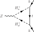
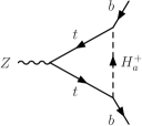
a)	b)

Figure 1: Two diagrams with charged scalars contributing to the $Zb\bar{b}$ vertex.

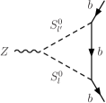
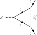
a)	b)

Figure 2: Two diagrams with neutral scalars contributing to the $Zb\bar{b}$ vertex.

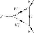
$a$)	$b$)
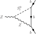
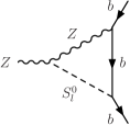
$c$)	$d$)

Figure 3: Diagrams referred as to “type d)” in Ref. [7].

The diagrams in Figs. 1 and 2 are divergent and must be renormalized. We follow the on-shell renormalization scheme of Hollik [29, 30]. Applying multiplicative renormalization, the renormalized vertex acquires some terms leading to a correction to the $Z$ propagator; these are part of the oblique parameters and were shown to be very small in Ref. [7]. Here we are looking for the terms that change the tree-level couplings, which after renormalization may be written as

$$i\hat{\Gamma}_{\mu}^{Zff}\!=\!-i\gamma_{\mu}\frac{g}{c_{W}}\!\left[\left(g_{Lb}^{0}+\Delta g_{L}\right)\!P_{L}\!+\left(g_{Rb}^{0}+\Delta g_{R}\right)\!P_{R}\right],$$ (14)

where $\Delta g_{\aleph}$ ($\aleph=L,R$) represent all the one-loop corrections after renormalization, including the ones involving $G^{\pm}$, $G^{0}$, and the already-observed neutral scalar with mass 125 GeV (more on this in Section 4). To perform the renormalization one needs to evaluate the renormalization constants that are obtained from the self-energies. We therefore need to evaluate the contributions of both the charged and neutral scalars to the self-energies, shown in Fig. 4. The self-energy $i\Sigma\left(p\right)$ receives contributions proportional to $\not\!pP_{L}$, $\not\!pP_{R}$, $m_{b}P_{L}$, and $m_{b}P_{R}$. In our approximation of neglecting $m_{b}$, we write

$$\Sigma(p)=\not\!p\left[\Omega_{L}\left(p^{2}\right)P_{L}+\Omega_{R}\left(p^{2}\right)P_{R}\right].$$ (15)

Following Hollik’s renormalization scheme [29, 30], the self-energy produces contributions to $\Delta g_{Lb}$ and $\Delta g_{Rb}$ given by

$$\Delta g_{Lb}\left(c\right) = -g_{Lb}^{0}\,\Omega_{L}\left(p^{2}=m_{b}^{2}\right),$$ (16a)

$$\Delta g_{Rb}\left(c\right) = -g_{Rb}^{0}\,\Omega_{R}\left(p^{2}=m_{b}^{2}\right).$$ (16b)

Note that Ref. [7] follows an equivalent procedure, ignoring renormalization and calculating simply the reducible diagrams with self-energy corrections in the external bottom quarks, which they dub “type c) diagrams”. Although we do perform the renormalization, we will name the contributions arising from it as “type c)”, allowing for an easy comparison with Ref. [7].

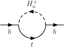
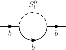
$a$)		$b$)

Figure 4: Contribution of the charged and neutral scalars to the self-energy of the bottom quark, leading to “type c)” contributions to the vertex.

Our calculations of the various diagrams have been performed by hand and then confirmed through the standard computer codes FeynRules [31], QGRAF [32], and FeynCalc [33, 34]. Recently, two of us (DF and JCR) have developed the new software FeynMaster [35] that handles, in an automated way, all these steps. The results involve Passarino–Veltman loop functions [36]; our conventions for them coincide with those in FeynCalc and LoopTools [37, 38], and are summarized in Appendix A.

We next turn to the computation of each diagram.

2.3 Calculating the diagrams involving charged scalars

The diagrams in Fig. 1a) lead to

$$\Delta g_{Lb}\left(a\right) = \frac{1}{8\pi^{2}}\sum_{a,a^{\prime}=1}^{n}c_{a}X_{aa^{\prime}}c_{a^{\prime}}^{\ast}\,C_{00}\left(M_{Z}^{2},0,0,m_{a^{\prime}}^{2},m_{a}^{2},m_{t}^{2}\right),$$ (17a)

$$\Delta g_{Rb}\left(a\right) = \Delta g_{Lb}\left(a\right)\left(c_{a}\rightarrow d_{a}^{\ast}\right),$$ (17b)

where $C_{00}$ is a Passarino–Veltman function defined through Eq. (116). We have set $m_{b}=0$ inside all the Passarino–Veltman functions; however, when evaluating them numerically it is sometimes better to keep $m_{b}\neq 0$ in order to avoid numerical instabilities. We should note that the sums in Eqs. (17) start at $a=1$, i.e. they include the charged Golsdtone bosons $G^{\pm}$. However, one may show that $X_{1a}=X_{a1}=0$, and therefore the sum in Eq. (17a) may start at $a,a^{\prime}=2$, while the term with $a=a^{\prime}=1$ is separately included in the SM contribution.

The diagrams in Fig. 1b) lead, after taking into account that

$$\left(d-2\right)C_{00}\left(\dots\right)=2\,C_{00}\left(\dots\right)-1/2$$

($d$ is the dimension of space–time), to

$$\Delta g_{Lb}\left(b\right) = \frac{1}{16\pi^{2}}\sum_{a=1}^{n}\left|c_{a}\right|^{2}\left\{{\vbox to14.0pt{}}-m_{t}^{2}\,g_{Lt}^{0}\,C_{0}\left(0,M_{Z}^{2},0,m_{a}^{2},m_{t}^{2},m_{t}^{2}\right)\right.$$ (18a)

$$+g_{Rt}^{0}\bigg{[}{\vbox to12.0pt{}}2\,C_{00}\left(0,M_{Z}^{2},0,m_{a}^{2},m_{t}^{2},m_{t}^{2}\right)-\frac{1}{2}$$

$$\left.-M_{Z}^{2}\,C_{12}\left(0,M_{Z}^{2},0,m_{a}^{2},m_{t}^{2},m_{t}^{2}\right){\vbox to12.0pt{}}\bigg{]}{\vbox to14.0pt{}}\right\}\!,$$

$$\Delta g_{Rb}\left(b\right) = \Delta g_{Lb}\left(b\right)\left(c_{a}\rightarrow d_{a},\ g_{Lt}^{0}\leftrightarrow g_{Rt}^{0}\right).$$ (18b)

The Passarino–Veltman function $C_{0}$ is defined in Eq. (114), while $C_{12}$ is defined through Eq. (116).

As for the type c) contributions, arising through renormalization from the diagram in Fig. 4a), we find

$$\Delta g_{Lb}\left(c\right) = \frac{g_{Lb}^{0}}{16\pi^{2}}\sum_{a=1}^{n}\left|c_{a}\right|^{2}B_{1}\left(0,m_{t}^{2},m_{a}^{2}\right),$$ (19a)

$$\Delta g_{Rb}\left(c\right) = \Delta g_{Lb}\left(c\right)\left(c_{a}\rightarrow d_{a},\ g_{Lb}^{0}\to g_{Rb}^{0}\right).$$ (19b)

The Passarino–Veltman function $B_{1}$ is defined in Eq. (113).

In the CP-conserving limit, Eqs. (17)–(19) agree with Eqs. (4.1) of Ref. [7], and also with Ref. [39].

The functions $B_{1}$ and $C_{00}$ are divergent; all the other Passarino–Veltman functions appearing in this paper are finite. In dimensional regularization, defining the divergent quantity

$$\textrm{div}=\frac{2}{4-d}-\gamma+\ln{\left(4\pi\right)},$$ (20)

one has

$$B_{1}\left(r^{2},m_{0}^{2},m_{1}^{2}\right) = -\frac{\textrm{div}}{2}+\mathrm{finite\ terms},$$ (21a)

$$C_{00}\left[r_{1}^{2},\left(r_{1}-r_{2}\right)^{2},r_{2}^{2},m_{0}^{2},m_{1}^{2},m_{2}^{2}\right] = +\frac{\textrm{div}}{4}+\mathrm{finite\ terms}.$$ (21b)

Therefore, the divergent terms in Eqs. (17)–(19) are

$$\Delta g_{Lb}\left(a\right)+\Delta g_{Lb}\left(b\right)+\Delta g_{Lb}\left(c\right)$$

$$= \frac{\textrm{div}}{32\pi^{2}}\left[\sum_{a,a^{\prime}=1}^{n}c_{a}X_{aa^{\prime}}c_{a^{\prime}}^{\ast}+\left(g_{Rt}^{0}-g_{Lb}^{0}\right)\sum_{a=1}^{n}\left|c_{a}\right|^{2}\right]+\cdots,$$

$$\Delta g_{Rb}\left(a\right)+\Delta g_{Rb}\left(b\right)+\Delta g_{Rb}\left(c\right)$$

$$= \frac{\textrm{div}}{32\pi^{2}}\left[\sum_{a,a^{\prime}=1}^{n}d_{a}^{\ast}X_{aa^{\prime}}d_{a^{\prime}}+\left(g_{Lt}^{0}-g_{Rb}^{0}\right)\sum_{a=1}^{n}\left|d_{a}\right|^{2}\right]+\cdots.$$ (22b)

We thus conclude that in any sensible theory one must have

$$\sum_{a,a^{\prime}}c_{a}X_{aa^{\prime}}c_{a^{\prime}}^{\ast} = \frac{s_{W}^{2}-c_{W}^{2}}{2}\sum_{a}\left|c_{a}\right|^{2},$$ (23a)

$$\sum_{a,a^{\prime}}d_{a}^{\ast}X_{aa^{\prime}}d_{a^{\prime}} = \frac{s_{W}^{2}-c_{W}^{2}}{2}\sum_{a}\left|d_{a}\right|^{2},$$ (23b)

where we have used Eq. (8).

2.4 Calculating the diagrams involving neutral scalars

The diagrams in Fig. 2a) lead to

$$\Delta g_{Lb}\left(a\right) = \frac{i}{4\pi^{2}}\sum_{l,l^{\prime}=1}^{m}r_{l}Y_{ll^{\prime}}r_{l^{\prime}}^{\ast}\,C_{00}\left(0,M_{Z}^{2},0,0,m_{l^{\prime}}^{2},m_{l}^{2}\right),$$ (24a)

$$\Delta g_{Rb}\left(a\right) = \Delta g_{Lb}\left(a\right)\left(r_{l}\rightarrow r_{l}^{\ast}\right).$$ (24b)

The diagrams in Fig. 2b) lead to

$$\Delta g_{Lb}\left(b\right)= \,\frac{g_{Rb}^{0}}{16\pi^{2}}\sum_{l=1}^{m}\left|r_{l}\right|^{2}\bigg{[}2\,C_{00}\left(0,M_{Z}^{2},0,m_{l}^{2},0,0\right)-\frac{1}{2}$$

$$\hskip 28.45274pt-M_{Z}^{2}\,C_{12}\left(0,M_{Z}^{2},0,m_{l}^{2},0,0\right)\bigg{]},$$ (25a)

$$\Delta g_{Rb}\left(b\right)= \,\Delta g_{Lb}\left(b\right)\left(g_{Rb}^{0}\to g_{Lb}^{0}\right).$$ (25b)

As for the type c) contributions, arising through renormalization from Fig. 4b), we find

$$\Delta g_{Lb}\left(c\right) = \frac{g_{Lb}^{0}}{16\pi^{2}}\sum_{l=1}^{m}\left|r_{l}\right|^{2}B_{1}\left(0,0,m_{l}^{2}\right),$$ (26a)

$$\Delta g_{Rb}\left(c\right) = \Delta g_{Lb}\left(c\right)\left(g_{Lb}^{0}\rightarrow g_{Rb}^{0}\right).$$ (26b)

In the CP-conserving limit, Eqs. (24)–(26) agree with Eqs. (5.1) of Ref. [7].

Collecting all the divergent terms in Eqs. (24a), (25a), and (26a) we find

$$\Delta g_{Lb}\left(a\right)+\Delta g_{Lb}\left(b\right)+\Delta g_{Lb}\left(c\right)$$ (27)

$$= \frac{\textrm{div}}{32\pi^{2}}\left[2i\sum_{l,l^{\prime}=1}^{m}r_{l}Y_{ll^{\prime}}r_{l^{\prime}}^{\ast}+\left(g_{Rb}^{0}-g_{Lb}^{0}\right)\sum_{l=1}^{m}\left|r_{l}\right|^{2}\right]+\cdots.$$

Since $g_{Rb}^{0}-g_{Lb}^{0}=1/2$, a consistent theory requires

$$\sum_{l,l^{\prime}=1}^{m}r_{l}Y_{ll^{\prime}}r_{l^{\prime}}^{*}=\frac{i}{4}\sum_{l}|r_{l}|^{2}.$$ (28)

This condition can also be obtained by collecting all the divergent terms in Eqs. (24b), (25b), and (26b).

The diagrams in Fig. 3c),d) involve neutral scalars. They are not divergent and they are suppressed by $m_{b}$. However, we keep them because they might be enhanced when the coupling of neutral scalars to the bottom quark gets enhanced, as in the type-II 2HDM. From them we get

$$\Delta g_{Lb}\left(d\right) = \frac{gm_{b}M_{Z}}{8\pi^{2}c_{W}}\sum_{l=1}^{m}y_{l}\,\mathrm{Re}\,r_{l}\left\{{\vbox to14.0pt{}}g_{Lb}^{0}\Big{[}C_{0}\left(M_{Z}^{2},0,0,M_{Z}^{2},m_{l}^{2},0\right)\right.$$ (29a)

$$\left.\hskip 85.35826pt-C_{1}\left(M_{Z}^{2},0,0,M_{Z}^{2},m_{l}^{2},0\right)\Big{]}\right.$$

$$\left.\hskip 85.35826pt+g_{Rb}^{0}\,C_{1}\left(M_{Z}^{2},0,0,m_{l}^{2},M_{Z}^{2},0\right){\vbox to14.0pt{}}\right\},\hskip 14.22636pt$$

$$\Delta g_{Rb}\left(d\right) = \Delta g_{Lb}\left(d\right)\left(g_{Lb}^{0}\leftrightarrow g_{Rb}^{0}\right).$$ (29b)

The function $C_{1}$ is defined through Eq. (115).

At this juncture we want to make a clarification. The one-loop results for $\Delta g_{Lb}$ and $\Delta g_{Rb}$ have imaginary parts. If there are no scalars with mass below $M_{Z}/2$, then the imaginary parts only appear through cuts of the internal bottom-quark lines of Fig. 2b), thus affecting only the contributions with neutral scalars. Although those imaginary parts may be of the same order of magnitude as the real parts, they are unimportant because the observables will depend on, for example,

$$\left|g_{Lb}\right|^{2} = \left|g_{Lb}^{0}+\Delta g_{Lb}\right|^{2}$$ (30)

$$= \left|g_{Lb}^{0}\right|^{2}+2\,\textrm{Re}\left(g_{Lb}^{0}\,\Delta g_{Lb}^{\ast}\right)+\mathrm{O}\left(\Delta g_{Lb}^{2}\right)$$

$$= \left|g_{Lb}^{0}\right|^{2}+2\,g_{Lb}^{0}\,\textrm{Re}\left(\Delta g_{Lb}\right)+\mathrm{O}\left(\Delta g_{Lb}^{2}\right),$$

where the last line follows from the fact that $g_{Lb}^{0}$ is real. As a result, the impact of an imaginary $\Delta g_{Lb}$ on the observables (see the next section) effectively appears only at higher order.

2.5 Summary

A generic theory with the couplings in Eqs. (1), (5), (6), and (9)–(13) gets radiative corrections to the $Zb\bar{b}$ vertex, obtained at the one-loop level by summing our Eqs. (17a), (18a), (19a), (24a), (25a), and (26a)—and, if enhanced, (29a)—for $\Delta g_{Lb}$, and by summing our Eqs. (17b), (18b), (19b), (24b), (25b), and (26b)—and, if enhanced, (29b)—for $\Delta g_{Rb}$. The theory only makes sense if its couplings are related through Eqs. (23a), (23b), and (28), which are needed in order for the divergences to cancel.

3 Models with doublet and singlet scalars

We now focus on extensions of the SM with $n_{d}$ scalar doublets, $n_{c}$ singly-charged scalar $SU(2)_{L}$ singlets, and $n_{n}$ real scalar gauge-invariant fields. The particle content is then $2n\equiv 2\left(n_{d}+n_{c}\right)$ charged scalars $H_{a}^{\pm}$ and $m\equiv 2n_{d}+n_{n}$ neutral scalars $S_{l}^{0}$; this counting includes the Goldstone bosons $H_{1}^{\pm}=G^{\pm}$ and $S_{1}^{0}=G^{0}$. Without loss of generality, one may assume that the scalar with mass 125 GeV found at the LHC is $S^{0}_{2}$; generality is lost if one makes the further assumption that the masses are ordered, since there might be massive scalar(s) below 125 GeV.

The scalar doublets are

$$\Phi_{k}=\left(\begin{array}[]{c}\varphi_{k}^{+}\\[2.84526pt] \varphi_{k}^{0}\end{array}\right),\quad\quad\tilde{\Phi}_{k}\equiv i\sigma_{2}\Phi_{k}^{\ast}=\left(\begin{array}[]{c}{\varphi_{k}^{0}}^{\ast}\\[2.84526pt] -\varphi_{k}^{-}\end{array}\right).$$ (31)

The fields $\varphi_{k}^{0}$ have VEVs $v_{k}\left/\sqrt{2}\right.$, where the $v_{k}$ may be complex.

Obviously, the charged and neutral $SU(2)_{L}$ singlets have no Yukawa couplings. The Yukawa Lagrangian is

$$\begin{split}\mathcal{L}_{\textrm{Yukawa}}=-\left(\begin{array}[]{cc}\overline{t_{L}}&\overline{b_{L}}\end{array}\right)\sum_{k=1}^{n_{d}}\Bigg{[}&f_{k}\left(\begin{array}[]{c}\varphi_{k}^{+}\\[5.69054pt] \varphi_{k}^{0}\end{array}\right)b_{R}+e_{k}\left(\begin{array}[]{c}{\varphi_{k}^{0}}^{\ast}\\[2.84526pt] -\varphi_{k}^{-}\end{array}\right)t_{R}\Bigg{]}+\textrm{H.c.},\end{split}$$ (32)

where the $e_{k}$ and the $f_{k}$ ($k=1,\ldots,n_{d}$) are the Yukawa coupling constants.

3.1 Formalism

We use the formalism in Refs. [25, 26, 27]. We write $\varphi_{k}^{+}$ and $\varphi_{k}^{0}$ as superpositions of the physical (i.e. eigenstates of mass) fields as

$$\varphi_{k}^{+} = \sum_{a=1}^{n}\mathcal{U}_{ka}H_{a}^{+},$$ (33)

$$\varphi_{k}^{0} = \frac{1}{\sqrt{2}}\left(v_{k}+\sum_{l=1}^{m}\mathcal{V}_{kl}S_{l}^{0}\right).$$ (34)

The matrix $\mathcal{U}$ is $n_{d}\times n$ and the matrix $\mathcal{V}$ is $n_{d}\times m$.

Since $H_{1}^{\pm}$ and $S_{1}^{0}$ are Goldstone bosons, the first columns of $\mathcal{U}$ and $\mathcal{V}$ are fixed and given by

$$\mathcal{U}_{k1}=\frac{v_{k}}{v},\quad\quad\mathcal{V}_{k1}=\frac{iv_{k}}{v},$$ (35)

where $v^{2}\equiv\sum_{k=1}^{n_{d}}|v_{k}|^{2}$ ($v$ is real and positive by definition).

There is an $n\times n$ matrix

$$\tilde{\mathcal{U}}=\left(\begin{array}[]{c}\mathcal{U}\\ \mathcal{T}\end{array}\right)$$ (36)

that is unitary, implying that

$$\mathcal{U}\mathcal{U}^{\dagger}=\mathbbm{1}_{n_{d}\times n_{d}}.$$ (37)

The matrix $\mathcal{T}$ in Eq. (36) only exists when the number $n_{c}$ of charged scalar $SU(2)_{L}$ singlets is nonzero. There is an $m\times m$ matrix

$$\tilde{\mathcal{V}}=\left(\begin{array}[]{c}\mathrm{Re}\,\mathcal{V}\\ \mathrm{Im}\,\mathcal{V}\\ \mathcal{R}\end{array}\right)$$ (38)

that is real and orthogonal. Therefore,

$$\textrm{Re}\,\mathcal{V}\ \textrm{Re}\,\mathcal{V}^{T} = \mathbbm{1}_{n_{d}\times n_{d}},$$ (39a)

$$\textrm{Im}\,\mathcal{V}\ \textrm{Im}\,\mathcal{V}^{T} = \mathbbm{1}_{n_{d}\times n_{d}},$$ (39b)

$$\textrm{Re}\,\mathcal{V}\ \textrm{Im}\,\mathcal{V}^{T} = 0_{n_{d}\times n_{d}},$$ (39c)

$$\textrm{Im}\,\mathcal{V}\ \textrm{Re}\,\mathcal{V}^{T} = 0_{n_{d}\times n_{d}}.$$ (39d)

The matrix $\mathcal{R}$ in Eq. (38) only exists in models with $n_{n}\neq 0$.

One can show [26] that in this class of models

$$X_{aa^{\prime}} = s_{W}^{2}\delta_{aa^{\prime}}-\frac{\left(\mathcal{U}^{T}\mathcal{U}^{\ast}\right)_{aa^{\prime}}}{2},$$ (40)

$$= \frac{s_{W}^{2}-c_{W}^{2}}{2}\,\delta_{aa^{\prime}}+\frac{\left(\mathcal{T}^{T}\mathcal{T}^{\ast}\right)_{aa^{\prime}}}{2},$$ (41)

$$Y_{ll^{\prime}} = -\frac{1}{4}\,\textrm{Im}\left(\mathcal{V}^{\dagger}\mathcal{V}\right)_{ll^{\prime}}.$$ (42)

Moreover,

$$y_{l}=-\textrm{Im}\left(\mathcal{V}^{\dagger}\mathcal{V}\right)_{1l},$$ (43)

leading to $y_{l=1}=0$, because $\mathcal{V}^{\dagger}\mathcal{V}$ is Hermitian and therefore $\textrm{Im}\left(\mathcal{V}^{\dagger}\mathcal{V}\right)_{11}=0$. Thus, the sum in Eq. (13) really starts at $l=2$, viz. there is no vertex $ZZG^{0}$, just as there is no vertex $ZZZ$.

3.2 Cancellation of the divergences

It follows from Eqs. (9), (10), and (32)–(34) that

$$c_{a} = \sum_{k=1}^{n_{d}}\mathcal{U}_{ka}^{\ast}e_{k}=\left(\mathcal{U}^{\dagger}E\right)_{a},$$ (44)

$$d_{a} = \sum_{k=1}^{n_{d}}\mathcal{U}_{ka}f_{k}=\left(\mathcal{U}^{T}F\right)_{a},$$ (45)

$$r_{l} = -\frac{1}{\sqrt{2}}\sum_{k=1}^{n_{d}}\mathcal{V}_{kl}f_{k}=-\frac{1}{\sqrt{2}}\left(\mathcal{V}^{T}F\right)_{l},$$ (46)

where we have defined the $n_{d}\times 1$ vectors

$$E=\left(\begin{array}[]{c}e_{1}\\ e_{2}\\ \vdots\\ e_{n_{d}}\end{array}\right),\quad\quad F=\left(\begin{array}[]{c}f_{1}\\ f_{2}\\ \vdots\\ f_{n_{d}}\end{array}\right).$$ (47)

From Eqs. (35) and (44)–(46),

$$\left|c_{1}\right| = \left|\sum_{k=1}^{n_{d}}\frac{v_{k}^{\ast}}{v}\,e_{k}\right|=\frac{\sqrt{2}m_{t}}{v},$$ (48a)

$$\left|d_{1}\right| = \left|\sum_{k=1}^{n_{d}}\frac{v_{k}}{v}\,f_{k}\right|=\frac{\sqrt{2}m_{b}}{v}\equiv 0,$$ (48b)

$$\left|r_{1}\right| = \left|\frac{1}{\sqrt{2}}\,\frac{v_{k}}{v}\,f_{k}\right|=\frac{m_{b}}{v}\equiv 0.$$ (48c)

We further define the $m\times 1$ column vector

$$R=\left(\begin{array}[]{c}r_{1}\\ r_{2}\\ \vdots\\ r_{m}\end{array}\right).$$ (49)

It then follows from Eq. (46) that

$$\sum_{l=1}^{m}\left|r_{l}\right|^{2} = \frac{1}{2}\,F^{T}\mathcal{V}\mathcal{V}^{\dagger}F^{\ast}$$

$$= \frac{1}{2}\,F^{T}\left(\mathrm{Re}{\mathcal{V}}+i\,\mathrm{Im}{\mathcal{V}}\right)\left(\mathrm{Re}{\mathcal{V}}^{T}-i\,\mathrm{Im}{\mathcal{V}}^{T}\right)F^{\ast}$$

$$= \frac{1}{2}\,F^{T}\Big{(}\mathrm{Re}{\mathcal{V}}\,\mathrm{Re}{\mathcal{V}}^{T}+\mathrm{Im}{\mathcal{V}}\,\mathrm{Im}{\mathcal{V}}^{T}+i\,\mathrm{Im}{\mathcal{V}}\,\mathrm{Re}{\mathcal{V}}^{T}-i\,\mathrm{Re}{\mathcal{V}}\,\mathrm{Im}{\mathcal{V}}^{T}\Big{)}F^{\ast}.$$

We now use Eqs. (39) to obtain

$$\sum_{l=1}^{m}\left|r_{l}\right|^{2} = \frac{1}{2}\,F^{T}\Big{(}\mathbbm{1}_{n_{d}\times n_{d}}+\mathbbm{1}_{n_{d}\times n_{d}}+i\times 0_{n_{d}\times n_{d}}-i\times 0_{n_{d}\times n_{d}}\Big{)}F^{\ast}$$ (51)

$$= F^{T}F^{\ast}=\sum_{k=1}^{n_{d}}\left|f_{k}\right|^{2}.$$

From Eqs. (44) and (37),

$$\sum_{a=1}^{n}|c_{a}|^{2}=E^{\dagger}\mathcal{U}\mathcal{U}^{\dagger}E=E^{\dagger}E=\sum_{k=1}^{n_{d}}|e_{k}|^{2}.$$ (52)

Notice that the two sums in Eq. (52) run over different spaces (up to $n$ and $n_{d}$, respectively). Similarly,

$$\sum_{a=1}^{n}|d_{a}|^{2}=\sum_{k=1}^{n_{d}}|f_{k}|^{2}.$$ (53)

From Eqs. (40), (44), and (37),

$$\sum_{a,a^{\prime}=1}^{n}c_{a}X_{aa^{\prime}}c_{a^{\prime}}^{\ast}\, = s_{W}^{2}\,E^{T}\mathcal{U}^{\ast}\mathcal{U}^{T}E^{\ast}-\frac{E^{T}\mathcal{U}^{\ast}\mathcal{U}^{T}\mathcal{U}^{\ast}\mathcal{U}^{T}E^{\ast}}{2}$$ (54)

$$= s_{W}^{2}\,E^{T}E^{\ast}-\frac{E^{T}E^{\ast}}{2}$$

$$= \frac{s_{W}^{2}-c_{W}^{2}}{2}\sum_{k=1}^{n_{d}}\left|e_{k}\right|^{2}$$

$$= \frac{s_{W}^{2}-c_{W}^{2}}{2}\sum_{a=1}^{n}\left|c_{a}\right|^{2},$$

where the last equality follows from Eq. (52). This proves that this class of models obeys the consistency Eq. (23a). Similarly, one can show that Eq. (23b) is also obeyed, confirming within this class of models the cancellation of the divergences of the contributions from charged scalars.

Next we compute

$$\sum_{l,l^{\prime}=1}^{m}r_{l}\,\mathrm{Im}{\left(\mathcal{V}^{\dagger}\mathcal{V}\right)_{ll^{\prime}}}\,r_{l^{\prime}}^{\ast} = \frac{1}{2}\,F^{T}\mathcal{V}\ \mathrm{Im}\Big{[}\left(\mathrm{Re}{\mathcal{V}}^{T}-i\,\mathrm{Im}{\mathcal{V}}^{T}\right)\left(\mathrm{Re}{\mathcal{V}}+i\,\mathrm{Im}{\mathcal{V}}\right)\Big{]}\mathcal{V}^{\dagger}F^{\ast}$$ (55)

$$= \frac{1}{2}\,F^{T}\left(\mathrm{Re}{\mathcal{V}}+i\,\mathrm{Im}{\mathcal{V}}\right)\left(\mathrm{Re}{\mathcal{V}}^{T}\,\mathrm{Im}{\mathcal{V}}-\mathrm{Im}{\mathcal{V}}^{T}\,\mathrm{Re}{\mathcal{V}}\right)$$

$$\qquad\times\left(\mathrm{Re}{\mathcal{V}}^{T}-i\,\mathrm{Im}{\mathcal{V}}^{T}\right)F^{\ast}.$$

We use once again Eqs. (39) to obtain

$$\sum_{l,l^{\prime}=1}^{m}r_{l}\,\mathrm{Im}{\left(\mathcal{V}^{\dagger}\mathcal{V}\right)_{ll^{\prime}}}\,r_{l^{\prime}}^{\ast} = \frac{1}{2}\,F^{T}\left(\mathrm{Im}{\mathcal{V}}-i\,\mathrm{Re}{\mathcal{V}}\right)\times\left(\mathrm{Re}{\mathcal{V}}^{T}-i\,\mathrm{Im}{\mathcal{V}}^{T}\right)F^{\ast}$$ (56)

$$= \frac{1}{2}\,F^{T}\left(-2i\times\mathbbm{1}_{n_{d}\times n_{d}}\right)F^{\ast}$$

$$= -i\,F^{T}F^{\ast}$$

$$= -i\,\sum_{k=1}^{n_{d}}\left|f_{k}\right|^{2}$$

$$= -i\,\sum_{l=1}^{m}\left|r_{l}\right|^{2},$$

where in the last step we have used Eq. (51). Taking into account Eq. (42), we conclude that in this class of models the consistency Eq. (28) also holds.

3.3 Simplification of the charged-scalars contribution

In this class of models, from Eqs. (41) and (8),

$$\begin{split}X_{aa^{\prime}}&=\left(g_{Lb}^{0}-g_{Rt}^{0}\right)\delta_{aa^{\prime}}+\frac{\left(\mathcal{T}^{T}\mathcal{T}^{\ast}\right)_{aa^{\prime}}}{2}\\ &=\left(g_{Rb}^{0}-g_{Lt}^{0}\right)\delta_{aa^{\prime}}+\frac{\left(\mathcal{T}^{T}\mathcal{T}^{\ast}\right)_{aa^{\prime}}}{2}.\end{split}$$

Therefore, one may write the charged-scalars contribution as

$$\left(16\pi^{2}\right)\Delta g_{Lb}=\sum_{a=1}^{n}\left|c_{a}\right|^{2}\left\{{\vbox to18.0pt{}}-g_{Lt}^{0}m_{t}^{2}C_{0}\left(0,M_{Z}^{2},0,m_{a}^{2},m_{t}^{2},m_{t}^{2}\right)\right.$$

$$+g_{Rt}^{0}\bigg{[}2\,C_{00}\left(0,M_{Z}^{2},0,m_{a}^{2},m_{t}^{2},m_{t}^{2}\right)-\frac{1}{2}-2\,C_{00}\left(0,M_{Z}^{2},0,m_{t}^{2},m_{a}^{2},m_{a}^{2}\right)$$

$$\hskip 43.05542pt-M_{Z}^{2}\,C_{12}\left(0,M_{Z}^{2},0,m_{a}^{2},m_{t}^{2},m_{t}^{2}\right)\bigg{]}$$

$$\left.+g_{Lb}^{0}\Big{[}B_{1}\left(0,m_{t}^{2},m_{a}^{2}\right)+2\,C_{00}\left(0,M_{Z}^{2},0,m_{t}^{2},m_{a}^{2},m_{a}^{2}\right)\Big{]}{\vbox to18.0pt{}}\right\}$$

$$+\!\!\sum_{a,a^{\prime}=1}^{n}\left(\mathcal{T}^{T}\mathcal{T}^{\ast}\right)_{aa^{\prime}}c_{a}c_{a^{\prime}}^{\ast}\,C_{00}\left(0,M_{Z}^{2},0,m_{t}^{2},m_{a^{\prime}}^{2},m_{a}^{2}\right).$$ (57)

The first column of the matrix $\mathcal{T}$ is zero, because $\sum_{k}\left|\mathcal{U}_{k1}\right|^{2}=\left.\sum_{k}\left|v_{k}\right|^{2}\right/v^{2}=1$. Thus, $\left(\mathcal{T}^{T}\mathcal{T}^{\ast}\right)_{1a}=\left(\mathcal{T}^{T}\mathcal{T}^{\ast}\right)_{a1}=0$ and the charged Goldstone boson does not contribute to the sum in the last line of Eq. (57). On the other hand, the Goldstone boson does contribute to the sum over $a$ in the first five lines, but $\left|c_{1}\right|$ has the same value as in the SM, cf. Eq. (48a); therefore, the contribution of the charged Goldstone boson is the same as in the SM and should be subtracted out. The simplified expression for the charged-scalar contributions to $\Delta g_{Rb}$ is obtained from Eq. (57) through the changes $c_{a}\to d_{a}^{\ast}$ and $L\leftrightarrow R$.

Suppose a model with no charged $SU(2)_{L}$ singlets. Then the matrix $\mathcal{T}$ does not exist. If one furthermore makes the approximation $M_{Z}=0$, then the contribution of the charged scalars in Eq. (57) becomes

$$\left(16\pi^{2}\right)\Delta g_{Lb} = \sum_{a=1}^{n}\left|c_{a}\right|^{2}\left\{-g_{Lt}^{0}m_{t}^{2}C_{0}\left(0,0,0,m_{a}^{2},m_{t}^{2},m_{t}^{2}\right)\right.$$ (58)

$$+2g_{Rt}^{0}\left[C_{00}\left(0,0,0,m_{a}^{2},m_{t}^{2},m_{t}^{2}\right)-C_{00}\left(0,0,0,m_{t}^{2},m_{a}^{2},m_{a}^{2}\right)\right.$$

$$\left.-\frac{1}{4}\right]$$

$$\left.+g_{Lb}^{0}\left[B_{1}\left(0,m_{t}^{2},m_{a}^{2}\right)+2\,C_{00}\left(0,0,0,m_{t}^{2},m_{a}^{2},m_{a}^{2}\right)\right]{\vbox to18.0pt{}}\right\},$$

and similarly for $\Delta g_{Rb}$, with $c_{a}\rightarrow d_{a}$ and $L\leftrightarrow R$. One easily finds that

$$B_{1}\left(0,m_{t}^{2},m_{a}^{2}\right)+2\,C_{00}\left(0,0,0,m_{t}^{2},m_{a}^{2},m_{a}^{2}\right)=0,$$ (59)

and that

$$C_{00}\left(0,0,0,m_{a}^{2},m_{t}^{2},m_{t}^{2}\right)-C_{00}\left(0,0,0,m_{t}^{2},m_{a}^{2},m_{a}^{2}\right)-\frac{1}{4}$$ (60)

$$= \frac{m_{t}^{2}}{2}\,C_{0}\left(0,0,0,m_{a}^{2},m_{t}^{2},m_{t}^{2}\right).$$

Hence,

$$\left(16\pi^{2}\right)\Delta g_{Lb} = \sum_{a=1}^{n}\left|c_{a}\right|^{2}\left(g_{Rt}^{0}-g_{Lt}^{0}\right)m_{t}^{2}\,C_{0}\left(0,0,0,m_{a}^{2},m_{t}^{2},m_{t}^{2}\right)$$ (61a)

$$= -\sum_{a=1}^{n}\frac{\left|c_{a}\right|^{2}}{2}\,m_{t}^{2}\,C_{0}\left(0,0,0,m_{a}^{2},m_{t}^{2},m_{t}^{2}\right),$$

$$\left(16\pi^{2}\right)\Delta g_{Rb} = \sum_{a=1}^{n}\left|d_{a}\right|^{2}\left(g_{Lt}^{0}-g_{Rt}^{0}\right)m_{t}^{2}\,C_{0}\left(0,0,0,m_{a}^{2},m_{t}^{2},m_{t}^{2}\right)$$ (61b)

$$= +\sum_{a=1}^{n}\frac{\left|d_{a}\right|^{2}}{2}\,m_{t}^{2}\,C_{0}\left(0,0,0,m_{a}^{2},m_{t}^{2},m_{t}^{2}\right).$$

The dependence on $\theta_{W}$ disappeared! This must indeed happen because, in the limit $M_{Z}=0$, the $Z$ gauge boson is indistinguishable from the photon—since they are both massless—, and therefore the Weinberg angle loses its meaning and must disappear from any physically meaningful quantity. The function

$$m_{t}^{2}\,C_{0}\left(0,0,0,m_{a}^{2},m_{t}^{2},m_{t}^{2}\right)=\frac{x}{1-x}\left(1+\frac{\ln{x}}{1-x}\right),\quad\mbox{with}\ x=\frac{m_{t}^{2}}{m_{a}^{2}}$$ (62)

has been given in Eq. (4.5) of Ref. [7] and has been used in all the subsequent analyses, by many authors, of models with extra doublets (and possibly neutral singlets). In our more general result (57), though, we keep CP violation, we allow for charged singlets and we do not make $M_{Z}=0$.

As a consequence of Eqs. (61), in a 2HDM, where there is only one physical charged scalar,

$$\frac{\Delta g_{Lb}}{\left|c_{2}\right|^{2}}=-\frac{\Delta g_{Rb}}{\left|d_{2}\right|^{2}}.$$ (63)

In general, as long as there are no charged singlets and the approximation $M_{Z}\approx 0$ is good, $\Delta g_{Lb}$ and $\Delta g_{Rb}$ have opposite signs when the contribution of the neutral scalars is not taken into account.

4 Connection with experiment

The couplings $g_{Lb}$ and $g_{Rb}$ in Eq. (1) may be determined experimentally from:

1. The rate

   $$R_{b}=\frac{\Gamma\left(Z\rightarrow b\bar{b}\right)}{\Gamma\left(Z\rightarrow\textrm{hadrons}\right)}.$$ (64)

2. Several asymmetries, including

   1. the $Z$-pole forward–backward asymmetry measured at LEP1

      $$A_{FB}^{(0,f)}=\frac{\sigma\left(e^{-}\rightarrow b_{F}\right)-\sigma\left(e^{-}\rightarrow b_{B}\right)}{\sigma\left(e^{-}\rightarrow b_{F}\right)+\sigma\left(e^{-}\rightarrow b_{B}\right)}=\frac{3}{4}A_{e}A_{b},$$ (65)

      where $b_{F}$ ($b_{B}$) stands for final-state bottom quarks moving in the forward (backward) direction with respect to the direction of the initial-state electron;

   2. the left–right forward–backward asymmetry measured by the SLD Collaboration

      $$\begin{split}A_{LR}^{FB}\left(b\right)&=\frac{\sigma\!\left(e_{L}^{-}\!\rightarrow\!b_{F}\right)\!-\sigma\left(e_{L}^{-}\!\rightarrow\!b_{B}\right)\!-\sigma\left(e_{R}^{-}\!\rightarrow\!b_{F}\right)\!+\sigma\left(e_{R}^{-}\!\rightarrow\!b_{B}\right)}{\sigma\left(e_{L}^{-}\!\rightarrow\!b_{F}\right)\!+\sigma\left(e_{L}^{-}\!\rightarrow\!b_{B}\right)\!+\sigma\left(e_{R}^{-}\!\rightarrow\!b_{F}\right)\!+\sigma\left(e_{R}^{-}\!\rightarrow\!b_{B}\right)}\\ &=\frac{3}{4}A_{b},\end{split}$$ (66)

      where $e_{L}^{-}$ ($e_{R}^{-}$) are initial-state left-handed (right-handed) electrons.

Introducing the vector- and axial-vector bottom-quark couplings

$$v_{b}=g_{Lb}+g_{Rb},\quad\quad a_{b}=g_{Lb}-g_{Rb},\quad\quad\mbox{and}\quad\quad r_{b}=\frac{v_{b}}{a_{b}},$$ (67)

one has [7, 40]

$$R_{b} = \left(1+\frac{\Sigma}{s_{b}\,\eta^{\textrm{QCD}}\,\eta^{\textrm{QED}}}\right)^{-1},$$ (68)

$$A_{b} = \frac{2\,r_{b}\,\sqrt{1-4\mu_{b}}}{1-4\mu_{b}+\left(1+2\mu_{b}\right)r_{b}^{2}}.$$ (69)

In Eq. (68), $\eta^{\textrm{QCD}}=0.9953$ and $\eta^{\textrm{QED}}=0.99975$ are QCD and QED corrections, respectively. Moreover,

$$\mu_{b} = \frac{m_{b}\left(M_{Z}\right)^{2}}{M_{Z}^{2}},$$ (70)

$$s_{b} = \left(1-6\mu_{b}\right)a_{b}^{2}+v_{b}^{2},$$ (71)

$$\Sigma = \sum_{q=u,d,s,c}\left(a_{q}^{2}+v_{q}^{2}\right).$$ (72)

Neglecting $\mu_{b}\approx 10^{-3}$ and setting the QCD and QED corrections to unity, one gets

$$R_{b} \approx \frac{2\left(g_{Lb}^{2}+g_{Rb}^{2}\right)}{2\left(g_{Lb}^{2}+g_{Rb}^{2}\right)+\Sigma},$$ (73)

$$A_{b} \approx \frac{g_{Lb}^{2}-g_{Rb}^{2}}{g_{Lb}^{2}+g_{Rb}^{2}}.$$ (74)

Equation (74) with $b\rightarrow e$ defines the $A_{e}$ appearing in Eq. (65), which has also been determined experimentally.

The recent fit to the electroweak data by Erler and Freitas in Ref. [8] finds

$$R_{b}^{\textrm{fit}} = 0.21629\pm 0.00066,$$ (75a)

$$A_{b}^{\textrm{fit}} = 0.923\pm 0.020,$$ (75b)

to be compared with the SM values $R_{b}^{\textrm{SM}}=0.21582\pm 0.00002$ and $A_{b}^{\textrm{SM}}=0.9347$. Thus, the experimental $R_{b}$ is about $0.7\sigma$ above the SM value, while $A_{b}$ is about $0.6\sigma$ below the SM value. However, this good agreement only applies to the overall fit of many observables producing Eqs. (75). The measured values of the bottom-quark asymmetries by themselves alone reveal a much larger discrepancy; as pointed out in Ref. [8], extracting $A_{b}$ from $A_{FB}^{(0,b)}$ and using $A_{e}=0.1501\pm 0.0016$ leads to a result which is $3.1\sigma$ below the SM (the precise value of $A_{b}$ depends on which observables $A_{e}$ is extracted from), while combining $A_{FB}^{(0,b)}$ with $A_{LR}^{FB}$ leads to $A_{b}=0.899\pm 0.013$, which deviates from the SM value by $2.8\sigma$.

There are, thus, two possible approaches. The first one consists in taking as good the values (75) obtained from the SM fit and using $R_{b}^{\textrm{fit}}$ and $A_{b}^{\textrm{fit}}$ as constraints on New Physics (NP). The second one is seeking NP that might explain an $R_{b}$ just slightly above the SM, together with an $A_{b}$ that undershoots the SM by $2.8\sigma$.

It is convenient to switch from the parameterization in Eq. (14), which splits the couplings $g_{\aleph b}$ as $g_{\aleph b}^{0}+\Delta g_{\aleph b}$, where $g_{\aleph b}^{0}$ is the tree-level piece and $\Delta g_{\aleph b}$ is the one-loop piece, to the alternative parameterization

$$g_{\aleph b}=g_{\aleph b}^{\textrm{SM}}+\delta g_{\aleph b},$$ (76)

which splits them into the SM piece $g_{\aleph b}^{\textrm{SM}}$ (which includes the SM loop correction) and the NP piece $\delta g_{\aleph b}$. A simple rule of thumb can be obtained by expanding to first order in the deviations; one finds [7]

$$\delta R_{b} = -0.7785\,\delta g_{Lb}+0.1409\,\delta g_{Rb},$$ (77a)

$$\delta A_{b} = -0.2984\,\delta g_{Lb}-1.6234\,\delta g_{Rb}.$$ (77b)

This shows that, assuming (rather arbitrarily) $\delta g_{Rb}\approx-\delta g_{Lb}$, $\delta R_{b}$ is pulled down (up) and $\delta A_{b}$ is pulled up (down) by a positive (negative) $\delta g_{Lb}$. Inverting Eqs. (77) [7],

$$\delta g_{Lb} = -1.2433\,\delta R_{b}-0.1079\,\delta A_{b},$$ (78a)

$$\delta g_{Rb} = 0.2286\,\delta R_{b}-0.5962\,\delta A_{b}.$$ (78b)

If one wishes to follow the second approach above, viz. using NP to keep $R_{b}$ close to its SM value while reducing $A_{b}$ significantly, then one needs to get a small $\delta g_{Lb}$ together with a significant positive $\delta g_{Rb}$.

5 Simple particular cases

5.1 The 2HDM in an alignment limit

In the 2HDM, one may always employ the ‘Higgs basis’ for the scalar doublets $\Phi_{1,2}$; in that basis,

$$\Phi_{1}=\left(\begin{array}[]{c}G^{+}\\ \left(v+\rho_{1}+iG^{0}\right)\left/\sqrt{2}\right.\end{array}\right),\quad\Phi_{2}=\left(\begin{array}[]{c}H^{+}\\ \left(\rho_{2}+i\eta\right)\left/\sqrt{2}\right.\end{array}\right),$$ (79)

where $G^{+}=H_{1}^{+}$ and $G^{0}=S_{1}^{0}$ are the Goldstone bosons and $H^{+}=H_{2}^{+}$ is a physical charged scalar. Then, the Yukawa couplings $e_{1}$ and $f_{1}$ are simply

$$e_{1}=\frac{\sqrt{2}m_{t}}{v},\quad\quad f_{1}=\frac{\sqrt{2}m_{b}}{v},$$ (80)

which may be taken to be real and positive. In this section we shall assume that, for some unspecified reason, the neutral fields $\rho_{1,2}$ and $\eta$ in Eq. (79) coincide with the physical neutral scalars, viz. $S_{2}^{0}=\rho_{1}$, $S_{3}^{0}=\rho_{2}$, and $S_{4}^{0}=\eta$. We moreover assume that $S_{2}^{0}$ is the scalar particle discovered at the LHC, with mass $m_{2}=125$ GeV. That means, we assume an ‘alignment limit’ [41] of the 2HDM wherein $S_{2}^{0}$ couples to the gauge bosons and to the top and bottom quarks with exactly the same strength as the Higgs boson of the SM. The matrix $\mathcal{U}$ defined by Eq. (33) and the matrix $\mathcal{V}$ defined by Eq. (34) are

$$\mathcal{U}=\left(\begin{array}[]{cc}1&0\\ 0&1\end{array}\right),\quad\quad\mathcal{V}=\left(\begin{array}[]{cccc}i&1&0&0\\ 0&0&1&i\end{array}\right).$$ (81)

Since $\mathcal{U}$ is, in this case, the $2\times 2$ unit matrix, we have, from Eqs. (44) and (45), $c_{1}=e_{1}$, $c_{2}=e_{2}$, $d_{1}=f_{1}$, and $d_{2}=f_{2}$. The free parameters in our model are the mass $M_{H^{+}}$ of the charged scalar, the masses $m_{3}$ and $m_{4}$ of the two new neutral scalars $S_{3}^{0}$ and $S_{4}^{0}$, respectively, and the Yukawa couplings $c_{2}$ and $d_{2}$. Since there are no charged singlets,

$$X_{aa^{\prime}}=\frac{s_{W}^{2}-c_{W}^{2}}{2}\,\delta_{aa^{\prime}},$$ (82)

while, from the matrix $\mathcal{V}$ in Eq. (81),

$$\textrm{Im}\left(\mathcal{V}^{\dagger}\mathcal{V}\right) = \left(\begin{array}[]{cccc}0&-1&0&0\\ 1&0&0&0\\ 0&0&0&1\\ 0&0&-1&0\end{array}\right),$$ (83e)

$$R=\left(\begin{array}[]{c}r_{1}\\ r_{2}\\ r_{3}\\ r_{4}\end{array}\right) = -\frac{1}{\sqrt{2}}\left(\begin{array}[]{c}i\,d_{1}\\ d_{1}\\ d_{2}\\ i\,d_{2}\end{array}\right).$$ (83n)

5.1.1 Charged-scalar contribution

Let us denote by superscripts $c$ and $n$ the new-physics contributions to $\delta g_{Lb}$ and $\delta g_{Rb}$ coming from the charged and neutral scalars, respectively. In the charged-scalar sector of a generic 2HDM, the contribution of the charged Goldstone boson can be separated and included in the SM. The genuine new contribution is

$$\delta g_{Lb}^{c} = \frac{\left|c_{2}\right|^{2}}{16\pi^{2}}\left\{\left(s_{W}^{2}-c_{W}^{2}\right)C_{00}\left(0,M_{Z}^{2},0,m_{t}^{2},M_{H^{+}}^{2},M_{H^{+}}^{2}\right)\right.$$ (84a)

$$-g_{Lt}^{0}\,m_{t}^{2}\,C_{0}\left(0,M_{Z}^{2},0,M_{H^{+}}^{2},m_{t}^{2},m_{t}^{2}\right)$$

$$+g_{Rt}^{0}\left[2\,C_{00}\left(0,M_{Z}^{2},0,M_{H^{+}}^{2},m_{t}^{2},m_{t}^{2}\right)-\frac{1}{2}\right.$$

$$\left.\left.-M_{Z}^{2}\,C_{12}\left(0,M_{Z}^{2},0,M_{H^{+}}^{2},m_{t}^{2},m_{t}^{2}\right)\right]+g_{Lb}^{0}\,B_{1}\left(0,m_{t}^{2},M_{H^{+}}^{2}\right)\right\},\hskip 19.91692pt$$

$$\delta g_{Rb}^{c} = \frac{\left|d_{2}\right|^{2}}{16\pi^{2}}\left\{\left(s_{W}^{2}-c_{W}^{2}\right)C_{00}\left(0,M_{Z}^{2},0,m_{t}^{2},M_{H^{+}}^{2},M_{H^{+}}^{2}\right)\right.$$ (84b)

$$-g_{Rt}^{0}\,m_{t}^{2}\,C_{0}\left(0,M_{Z}^{2},0,M_{H^{+}}^{2},m_{t}^{2},m_{t}^{2}\right)$$

$$+g_{Lt}^{0}\left[2\,C_{00}\left(0,M_{Z}^{2},0,M_{H^{+}}^{2},m_{t}^{2},m_{t}^{2}\right)-\frac{1}{2}\right.$$

$$\left.\left.-M_{Z}^{2}\,C_{12}\left(0,M_{Z}^{2},0,M_{H^{+}}^{2},m_{t}^{2},m_{t}^{2}\right)\right]+g_{Rb}^{0}\,B_{1}\left(0,m_{t}^{2},M_{H^{+}}^{2}\right)\right\}.$$

If we plot $\delta g_{Lb}^{c}\left/\left|c_{2}\right|^{2}\right.$ and $\delta g_{Rb}^{c}\left/\left|d_{2}\right|^{2}\right.$, we get general results for any 2HDM. We have used LoopTools [37] to perform the numerical integrations contained in the Passarino–Veltman functions. The results are shown in Fig. 5.

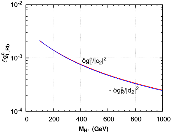
Figure 5: Contribution of the charged scalar to $\delta g_{Lb}$ (red curve) and to $-\delta g_{Rb}$ (blue curve) in a general 2HDM.

One sees that $0<\delta g_{Lb}^{c}\lesssim 0.002\left|c_{2}\right|^{2}$ and that Eq. (63) holds to an excellent approximation; this indicates that the approximation $M_{Z}=0$ is in fact very good. This is vindicated by Fig. 6, which displays the asymmetries $R_{g_{L,R}}$ between the values of $\delta g_{Lb}^{c}\left/\left|c_{2}\right|^{2}\right.$ and $\delta g_{Rb}^{c}\left/\left|d_{2}\right|^{2}\right.$ computed with $M_{Z}\neq 0$ and with $M_{Z}=0$:

$$R_{g_{L}}^{c} = \frac{\delta g_{Lb}^{c}\left(M_{Z}\right)-\delta g_{Lb}^{c}\left(0\right)}{\delta g_{Lb}^{c}\left(M_{Z}\right)+\delta g_{Lb}^{c}\left(0\right)},$$ (85a)

$$R_{g_{R}}^{c} = R_{g_{L}}^{c}\left(L\to R\right).$$ (85b)

One observes in Fig. 6 that both asymmetries are at most of order 1%.

Figure 6: In red: the asymmetry between $\delta g_{Lb}^{c}$ computed using $M_{Z}=91$ GeV and the same quantity computed using $M_{Z}=0$. In blue: the asymmetry between $\delta g_{Rb}^{c}$ computed with $M_{Z}=91$ GeV and the same quantity computed with $M_{Z}=0$.

5.1.2 Neutral-scalar contribution

Taking into account Eq. (42), in the class of models of Section 3, Eq. (24a) reads

$$\Delta g_{Lb}\left(a\right)=\frac{-i}{16\pi^{2}}\sum_{l,l^{\prime}=1}^{m}r_{l}\,\mathrm{Im}\left(\mathcal{V}^{\dagger}\mathcal{V}\right)_{ll^{\prime}}r_{l^{\prime}}^{\ast}\,C_{00}\left(0,M_{Z}^{2},0,0,m_{l^{\prime}}^{2},m_{l}^{2}\right).$$ (86)

Since $C_{00}\left(0,M_{Z}^{2},0,0,m_{l^{\prime}}^{2},m_{l}^{2}\right)=C_{00}\left(0,M_{Z}^{2},0,0,m_{l}^{2},\right.$ $\left.m_{l^{\prime}}^{2}\right),$ Eq. (86) may be simplified to

$$\Delta g_{Lb}\left(a\right)=\frac{1}{8\pi^{2}}\sum_{l=1}^{m-1}\sum_{l^{\prime}=l+1}^{m}\mathrm{Im}\left(\mathcal{V}^{\dagger}\mathcal{V}\right)_{ll^{\prime}}\,\mathrm{Im}\left(r_{l}r_{l^{\prime}}^{\ast}\right)C_{00}\left(0,M_{Z}^{2},0,0,m_{l^{\prime}}^{2},m_{l}^{2}\right).$$ (87)

In the 2HDM of this section, because of Eq. (83e), Eq. (87) reads

$$\Delta g_{Lb}\left(a\right) = \frac{1}{16\pi^{2}}\left[\left|d_{1}\right|^{2}C_{00}\left(0,M_{Z}^{2},0,0,m_{2}^{2},m_{1}^{2}\right)\right.$$ (88)

$$\left.-\left|d_{2}\right|^{2}C_{00}\left(0,M_{Z}^{2},0,0,m_{4}^{2},m_{3}^{2}\right)\right].$$

Since $S_{1}^{0}=G^{0}$ is the neutral Goldstone boson and $S_{2}^{0}$ is the Higgs particle of the SM, the first term in the right-hand side of Eq. (88) is an SM contribution that we are uninterested in; we just care about the NP contributions, which are

$$\delta g_{Lb}^{n} = \frac{\left|d_{2}\right|^{2}}{16\pi^{2}}\left\{-C_{00}\left(0,M_{Z}^{2},0,0,m_{3}^{2},m_{4}^{2}\right)\right.$$ (89a)

$$+\frac{g_{Rb}^{0}}{2}\left[2\,C_{00}\left(0,M_{Z}^{2},0,m_{3}^{2},0,0\right)-\frac{1}{2}-M_{Z}^{2}\,C_{12}\left(0,M_{Z}^{2},0,m_{3}^{2},0,0\right)\right.$$

$$\left.+2\,C_{00}\left(0,M_{Z}^{2},0,m_{4}^{2},0,0\right)-\frac{1}{2}-M_{Z}^{2}\,C_{12}\left(0,M_{Z}^{2},0,m_{4}^{2},0,0\right)\right]$$

$$\left.+\frac{g_{Lb}^{0}}{2}\left[B_{1}\left(0,0,m_{3}^{2}\right)+B_{1}\left(0,0,m_{4}^{2}\right)\right]\right\},$$

$$\delta g_{Rb}^{n} = \frac{\left|d_{2}\right|^{2}}{16\pi^{2}}\left\{C_{00}\left(0,M_{Z}^{2},0,0,m_{3}^{2},m_{4}^{2}\right)\right.$$ (89b)

$$+\frac{g_{Lb}^{0}}{2}\left[2\,C_{00}\left(0,M_{Z}^{2},0,m_{3}^{2},0,0\right)-\frac{1}{2}-M_{Z}^{2}\,C_{12}\left(0,M_{Z}^{2},0,m_{3}^{2},0,0\right)\right.$$

$$\left.+2\,C_{00}\left(0,M_{Z}^{2},0,m_{4}^{2},0,0\right)-\frac{1}{2}-M_{Z}^{2}\,C_{12}\left(0,M_{Z}^{2},0,m_{4}^{2},0,0\right)\right]$$

$$\left.+\frac{g_{Rb}^{0}}{2}\left[B_{1}\left(0,0,m_{3}^{2}\right)+B_{1}\left(0,0,m_{4}^{2}\right)\right]\right\}.$$

Let us compute the limit $M_{Z}=0$ of Eqs. (89). Using

$$C_{00}\left(0,0,0,0,A,B\right) = \frac{\mathrm{div}-\ln{\mu^{2}}}{4}+\frac{3}{8}+\frac{B\,\ln{B}-A\,\ln{A}}{4\left(A-B\right)},$$ (90a)

$$C_{00}\left(0,0,0,A,0,0\right)-\frac{1}{4} = -\frac{B_{1}\left(0,0,A\right)}{2},$$ (90b)

$$B_{1}\left(0,0,A\right) = -\frac{\mathrm{div}}{2}-\frac{1}{4}+\frac{1}{2}\,\ln{\frac{A}{\mu^{2}}},$$ (90c)

one obtains the approximation

$$\delta g_{Lb}^{n}\approx-\delta g_{Rb}^{n}\approx\frac{\left|d_{2}\right|^{2}}{64\pi^{2}}\left(-1+\frac{m_{3}^{2}+m_{4}^{2}}{m_{3}^{2}-m_{4}^{2}}\ln{\frac{m_{3}}{m_{4}}}\right),$$ (91)

which vanishes when $m_{3}=m_{4}$. One sees that

• in the limit $M_{Z}=0$, $\delta g_{Lb}^{n}=-\delta g_{Rb}^{n}$;

• in that limit, $\delta g_{Lb}^{n}$ and $\delta g_{Rb}^{n}$ are independent of $\theta_{W}$—this is for the reason explained after Eqs. (61);

• in that limit, $\delta g_{Lb}^{n}=\delta g_{Rb}^{n}=0$ when the two extra neutral scalars have equal masses.

We have evaluated the exact Eqs. (89) by using LoopTools [37]. We have checked in the numerical simulation that the divergences indeed cancel, by verifying that the results are independent of the $\Delta$ parameter of LoopTools. Without loss of generality, we have required that $m_{4}>m_{3}$. The results are shown in Fig. 7.

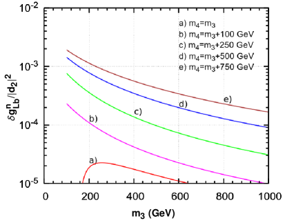
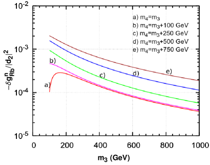
Figure 7: The contributions of the neutral scalars to $\delta g^{n}_{Lb}$ and $\delta g^{n}_{Rb}$ as functions of $m_{3}$, for different values of $m_{4}-m_{3}$.

It is seen that $\delta g_{Lb}^{n}>0$ but $\delta g_{Rb}^{n}<0$ (recall that a negative $\delta g_{Rb}$ goes in the wrong direction if one wishes to explain $A_{b}$ below the SM value); both are typically $\mathrm{O}\left(10^{-4}\right)\left|d_{2}\right|^{2}$ unless $m_{3}\sim 200$ GeV and $m_{4}\sim 1$ TeV, in which case they may reach $\mathrm{O}\left(10^{-3}\right)\left|d_{2}\right|^{2}$.

Comparing Figs. 5 and 7, one sees that, unless the masses of the two NP neutral scalars are close to each other, there is in general no rationale for neglecting the neutral-scalar contribution as compared to the charged-scalar one.

We have checked the validity of the approximation of neglecting $M_{Z}$ for the case of the neutral scalars. This is shown in Fig. 8.

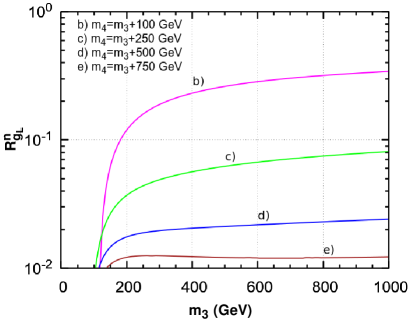
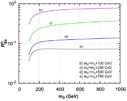
Figure 8: The asymmetries $R_{g_{Lb}}^{n}$ (left panel) and $R_{g_{Rb}}^{n}$ (right panel), defined in a fashion analogous to Eqs. (85), plotted as functions of $m_{3}$ for various values of $m_{4}-m_{3}$.

We see that the relative error of neglecting $M_{Z}$ is much larger in the case of the neutral scalars than in the case of the charged scalars (cf. Fig. 6), and it is larger for $g_{R}$ than for $g_{L}$. (When $m_{3}=m_{4}$ the asymmetries are 1, because the approximate expression of Eq. (91) vanishes for $m_{3}=m_{4}$ while the exact results are nonzero. We have not displayed this case in Fig. 8, because it would correspond to the upper line in the axes box.) On the other hand, the relative error is large precisely when the absolute values of $\delta g_{Lb}$ and $\delta g_{Rb}$ are small, i.e. when the exact values are not very relevant anyway.

In the left panel of Fig. 9 we have displayed the impact of both the charged- and neutral-scalar contributions in the $A_{b}$–$R_{b}$ plane.

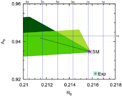
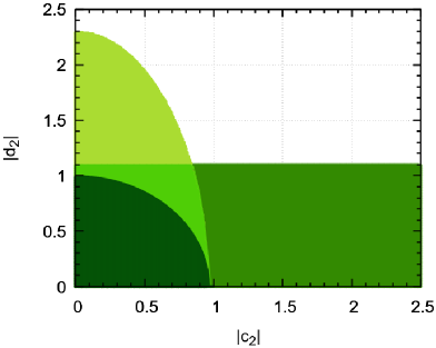
Figure 9: In making the left panel, we have used scalar masses $M_{H^{+}}=254$ GeV, $m_{3}=250$ GeV, and $m_{4}=850$ GeV, and we have let the Yukawa couplings $\left|c_{2}\right|$ and $\left|d_{2}\right|$ vary in between 0 and 2.5. We have depicted the values of $R_{b}$ and $A_{b}$ due to the charged-scalar contribution (in yellowish green), the neutral-scalar contribution (a straight line, because it is just a function of $\left|d_{2}\right|$), and the sum of both (in dark and bright green). We have also marked the experimental central point (green star), the various $n\sigma$ limits (blue lines), and the Standard Model prediction (violet star). In making the right panel, we have used the same scalar masses as for the left panel, and we have shown the impact of the $R_{b}$ $2\sigma$ limits on $\left|c_{2}\right|$ and $\left|d_{2}\right|$; the allowed ranges are depicted with only the charged-scalar contribution (yellowish and bright green), only the neutral-scalar contribution (horizontal band) and the sum of both (dark green).

In making Fig. 9, we have taken into account the experimental limits, $0.04<T<0.20$, on the electroweak parameter $T$. The contribution of the scalars to $T$ is

$$T=\frac{1}{16\pi s_{W}^{2}M_{W}^{2}}\left[f\left(M_{H^{+}},m_{3}\right)+f\left(M_{H^{+}},m_{4}\right)-f\left(m_{3},m_{4}\right)\right],$$ (92)

where $f\left(x,y\right)$ is the function

$$f(x,y)=\frac{x^{2}+y^{2}}{2}-\frac{x^{2}y^{2}}{x^{2}-y^{2}}\,\ln\frac{x^{2}}{y^{2}}.$$ (93)

The function $f$ is zero when $x=y$. In order to keep $T$ sufficiently small, we have set $M_{H}^{+}=254$ GeV rather close to $m_{3}=250$ GeV; on the other hand, we have set $m_{4}=850$ GeV much larger than $m_{3}$, so that $\delta g_{L,Rb}^{n}$ are rather large, cf. Fig. 7. We see that the impact on $A_{b}$ is always small, but the impact on $R_{b}$ may be quite strong when the Yukawa couplings $c_{2}$ and $d_{2}$ become large. This of course puts bounds on $\left|c_{2}\right|$ and $\left|d_{2}\right|$, and those bounds are displayed in the right panel of Fig. 9, using as input the $2\sigma$ experimental lower bound on $R_{b}$. We see that the impact of the neutral-scalar contributions can be quite drastic, cf. the large difference between the dark-green and light-green areas in the right panel of Fig. 9.

5.2 The complex 2HDM

The complex 2HDM (C2HDM) is a two-Higgs-doublet model with a softly broken $\mathbbm{Z}_{2}$ symmetry. The scalar potential is

$$V_{H} = m_{11}^{2}\,\Phi_{1}^{\dagger}\Phi_{1}+m_{22}^{2}\,\Phi_{2}^{\dagger}\Phi_{2}-m_{12}^{2}\,\Phi_{1}^{\dagger}\Phi_{2}-{m_{12}^{2}}^{\ast}\,\Phi_{2}^{\dagger}\Phi_{1}$$ (94)

$$+\frac{\lambda_{1}}{2}\,\Phi_{1}^{\dagger}\Phi_{1}\,\Phi_{1}^{\dagger}\Phi_{1}+\frac{\lambda_{2}}{2}\,\Phi_{2}^{\dagger}\Phi_{2}\,\Phi_{2}^{\dagger}\Phi_{2}+\lambda_{3}\,\Phi_{1}^{\dagger}\Phi_{1}\,\Phi_{2}^{\dagger}\Phi_{2}$$

$$+\lambda_{4}\,\Phi_{1}^{\dagger}\Phi_{2}\,\Phi_{2}^{\dagger}\Phi_{1}+\!\frac{\lambda_{5}}{2}\left(\Phi_{1}^{\dagger}\Phi_{2}\right)^{2}+\!\frac{\lambda_{5}^{\ast}}{2}\left(\Phi_{2}^{\dagger}\Phi_{1}\right)^{2}\!\!\!,$$

where all the parameters, except $m_{12}^{2}$ and $\lambda_{5}$, are real. In general, $\textrm{Im}\left[\left(m_{12}^{2}\right)^{2}\lambda_{5}^{\ast}\right]$ is allowed to be nonzero. By rephasing $\Phi_{1}$ and $\Phi_{2}$, we go to a basis where the VEVs are real and positive: $\left\langle 0\left|\varphi_{k}^{0}\right|0\right\rangle=v_{k}\left/\sqrt{2}\right.$ for $k=1,2$. We write

$$v_{1}=v\,c_{\beta},\quad\quad v_{2}=v\,s_{\beta},$$ (95)

where $v=246$ GeV and $0<\beta<\pi/2$. Thenceforth, $c_{\theta}$, $s_{\theta}$, and $t_{\theta}$ represent the cosine, sine, and tangent, respectively, of whatever angle $\theta$ is in the subindex. We write the scalar doublets as

$$\Phi_{k}=\left(\begin{array}[]{c}\varphi_{k}^{+}\\ \left(v_{k}+\eta_{k}+i\chi_{k}\right)\left/\sqrt{2}\right.\end{array}\right)\quad\quad(k=1,2).$$ (96)

We transform the fields into the so-called Higgs basis through [42]

$$\left(\begin{array}[]{c}H_{1}\\ H_{2}\end{array}\right)=\left(\begin{array}[]{cc}c_{\beta}&s_{\beta}\\ -s_{\beta}&c_{\beta}\end{array}\right)\left(\begin{array}[]{c}\Phi_{1}\\ \Phi_{2}\end{array}\right).$$ (97)

Then $H_{2}$ does not have a VEV:

$$H_{1} = \left(\begin{array}[]{c}G^{+}\\ \left(v+H^{0}+iG^{0}\right)\left/\sqrt{2}\right.\end{array}\right),$$ (98c)

$$H_{2} = \left(\begin{array}[]{c}H^{+}\\ \left(R_{2}+iI_{2}\right)\left/\sqrt{2}\right.\end{array}\right).$$ (98f)

$G^{+}$ and $G^{0}$ are the Goldstone bosons. There is a charged-scalar pair $H^{\pm}$ with mass $m_{H^{\pm}}$.

In a standard C2HDM notation, $\eta_{3}:=I_{2}$ and the neutral mass eigenstates are obtained from the three neutral components as

$$\left(\begin{array}[]{c}S^{0}_{2}\\[2.84526pt] S^{0}_{3}\\[2.84526pt] S^{0}_{4}\end{array}\right)=R\left(\begin{array}[]{c}\eta_{1}\\ \eta_{2}\\ \eta_{3}\end{array}\right).$$ (99)

The orthogonal matrix $R$ diagonalizes the neutral mass matrix

$$\left({\cal M}^{2}\right)_{ij}=\frac{\partial^{2}V_{H}}{\partial\eta_{i}\,\partial\eta_{j}},$$ (100)

through

$$R\,{\cal M}^{2}\,R^{T}=\textrm{diag}\left(m_{2}^{2},m_{3}^{2},m_{4}^{2}\right),$$ (101)

where $m_{2}=125\,\mathrm{GeV}\leq m_{3}\leq m_{4}$ are the masses of the neutral scalars ($m_{1}$ is the unphysical mass of the Goldstone boson $S^{0}_{1}=G^{0}$). In our numerical study we use $m_{3,4}\in\left[125\,\mathrm{GeV},\ 800\,\mathrm{GeV}\right]$ with $m_{3}<m_{4}$. We parameterize the orthogonal matrix $R$ as [43]

$$R=\left(\begin{array}[]{ccccc}c_{\alpha_{1}}c_{\alpha_{2}}&&s_{\alpha_{1}}c_{\alpha_{2}}&&s_{\alpha_{2}}\\ -s_{\alpha_{1}}c_{\alpha_{3}}-c_{\alpha_{1}}s_{\alpha_{2}}s_{\alpha_{3}}&&c_{\alpha_{1}}c_{\alpha_{3}}-s_{\alpha_{1}}s_{\alpha_{2}}s_{\alpha_{3}}&&c_{\alpha_{2}}s_{\alpha_{3}}\\ s_{\alpha_{1}}s_{\alpha_{3}}-c_{\alpha_{1}}s_{\alpha_{2}}c_{\alpha_{3}}&&-c_{\alpha_{1}}s_{\alpha_{3}}-s_{\alpha_{1}}s_{\alpha_{2}}c_{\alpha_{3}}&&c_{\alpha_{2}}c_{\alpha_{3}}\end{array}\right).$$ (102)

Without loss of generality, the angles may be restricted to [43]

$$-\pi/2<\alpha_{1}\leq\pi/2,\quad-\pi/2<\alpha_{2}\leq\pi/2,\quad 0\leq\alpha_{3}\leq\pi/2.$$ (103)

Taking the limit $\alpha_{2},\alpha_{3}\rightarrow 0$ one recovers a 2HDM with softly broken $\mathbbm{Z}_{2}$ symmetry and no CP violation; this is the ‘real 2HDM’, in which $S^{0}_{4}=A$ is the massive CP-odd scalar.

In practice, because of the experimental limit $1.1\times 10^{-29}$ e.cm on the electric dipole moment of the electron, both $\alpha_{1}$ and $\alpha_{2}$ are much more restricted than in inequalities (103): $\left|\alpha_{2}\right|\lesssim 0.1$ and $\alpha_{1}$ is always very close to $\beta$.

Comparing with Eqs. (33) and (34), we find

$$\mathcal{U} = \left(\begin{array}[]{cc}c_{\beta}&-s_{\beta}\\ s_{\beta}&c_{\beta}\end{array}\right),$$ (104c)

$$\mathcal{V} = \left(\begin{array}[]{cccc}ic_{\beta}&R_{11}-is_{\beta}R_{13}&R_{21}-is_{\beta}R_{23}&R_{31}-is_{\beta}R_{33}\\ is_{\beta}&R_{12}+ic_{\beta}R_{13}&R_{22}+ic_{\beta}R_{23}&R_{32}+ic_{\beta}R_{33}\end{array}\right).$$ (104f)

Equation (82) still holds and

$$\mathrm{Im}\left(\mathcal{V}^{\dagger}\mathcal{V}\right)$$ (109)

$$= {\footnotesize\left(\begin{array}[]{cccc}0&-c_{\beta}R_{11}-s_{\beta}R_{12}&-c_{\beta}R_{21}-s_{\beta}R_{22}&-c_{\beta}R_{31}-s_{\beta}R_{32}\\ c_{\beta}R_{11}+s_{\beta}R_{12}&0&c_{\beta}R_{31}+s_{\beta}R_{32}&-c_{\beta}R_{21}-s_{\beta}R_{22}\\ c_{\beta}R_{21}+s_{\beta}R_{22}&-c_{\beta}R_{31}-s_{\beta}R_{32}&0&c_{\beta}R_{11}+s_{\beta}R_{12}\\ c_{\beta}R_{31}+s_{\beta}R_{32}&c_{\beta}R_{21}+s_{\beta}R_{22}&-c_{\beta}R_{11}-s_{\beta}R_{12}&0\end{array}\right).}$$

Assuming the Yukawa couplings to follow the type-II 2HDM pattern, viz. $e_{1}=f_{2}=0$ and

$$e_{2}=\frac{\sqrt{2}m_{t}}{v_{2}},\quad\quad f_{1}=\frac{\sqrt{2}m_{b}}{v_{1}},$$ (111)

we have

$$c_{2}=\frac{\sqrt{2}m_{t}}{v}\cot{\beta},\quad\quad d_{2}=-\frac{\sqrt{2}m_{b}}{v}\tan{\beta}.$$ (112)

Note that, contrary to the assumptions in the previous subsection, here $\left|c_{2}\right|$ and $\left|d_{2}\right|$ may be of vastly different orders of magnitude—in particular, $\left|d_{2}\right|\ll\left|c_{2}\right|$ for $\tan{\beta}\sim 1$. However, when $\tan{\beta}\gtrsim\sqrt{m_{t}/m_{b}}\approx 6$, $\left|d_{2}\right|$ becomes larger than $\left|c_{2}\right|$, and that is the regime that we will be mostly interested in.

This model was studied in detail in Ref. [44], which introduced the code C2HDM_HDECAY implementing the C2HDM in HDECAY [45, 46]. For illustrative purposes, we take points from that fit, where, invoking constraints from Flavour Physics on $R_{b}$[7], $\tan{\beta}$ was taken above $0.8$. In that scan the following ranges were considered:

• $\tan\beta\in[0.8:35]$,

• $m_{2}=125\text{GeV},\ m_{3},m_{4}\in[125:800]\text{GeV\,}$,

• $M_{H^{+}}\in[580:800]\text{GeV\,}$,

where $m_{4}>m_{3}$ and the constraint on the charged Higgs mass comes from B-physics[47, 48, 49, 50] All points passed both the theoretical constraints on unitarity [51, 52], bounded from below, and the electroweak parameters $S,T,U$, as well the experimental constraints coming from the LHC. We combine these with the results from a new dedicated run $\tan{\beta}\in[0:100]$. Such extreme (very low and very high) values of $\tan{\beta}$ may be in contradiction with certain Flavour Physics observables, notably (as we will now show) $Z\rightarrow b\bar{b}$. Nevertheless, we will consider those extreme values since we wish to stress that the details of such a bound may require both the charged-scalar and the neutral-scalar contributions. As shown in Fig. 8 of Ref. [53], very large $\tan{\beta}$ is only consistent with current measurements at LHC if $\alpha_{1}$ lies in a very restricted range $\alpha_{1}\approx\beta$, which we impose in this run ab initio. Moreover, in order to obtain agreement with the measured EDMs, $\alpha_{2}$ always turns out to be very small.

As in the alignment case discussed previously, the contribution due to the charged Goldstone bosons decouples, it is included in the SM and subtracted out, and the result from charged scalars is still given by Eqs. (84) and Fig. 5. Note that $\delta g_{Lb}^{c}$ is positive while $\delta g_{Rb}^{c}$ is negative. Recall that the positive $\delta g_{Lb}$ tends to make $R_{b}$ smaller and from there comes a bound in the $m_{H^{\pm}}$–$\tan{\beta}$ plane. The correction $\delta g_{Rb}^{c}$ is too small to have an impact on $R_{b}$ (see Eq. (77a)) but it could have a substantial impact on $A_{b}$ going in the wrong direction when compared with the experimental measurements (see Eq. (77b)). However, we will see below (see the right panel of Fig. 12) that this only happens for large values of $\tan\beta$ not allowed by perturbativity.

We are particularly interested in the contributions to $\delta g_{Lb}$ and $\delta g_{Rb}$ arising from the neutral scalars, because in the literature they are frequently disconsidered. We would like to know under which circumstances those contributions can be large. We have separated the data of our scans in three different sets:

• Small $\tan\beta\in[0,10]$, blue in the plots.

• Intermediate $\tan\beta\in[10,30]$, green in the plots.

• Large $\tan\beta\in[30,100]$, red in the plots.

In the left panel of Fig. 10

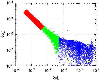
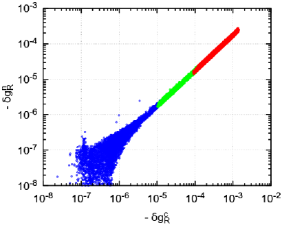
Figure 10: Comparison of $\delta g_{Lb}^{n}$ with $\delta g_{Lb}^{c}$ (left plot) and of $\delta g_{Rb}^{n}$ with $\delta g_{Rb}^{c}$ (right plot).

we display $\delta g_{Lb}^{n}$ versus $\delta g_{Lb}^{c}$ for all three sets; in the right panel, $-\delta g_{Rb}^{n}$ is displayed against $-\delta g_{Rb}^{c}$ (remember that both $\delta g_{Rb}^{n}$ and $\delta g_{Rb}^{c}$ are negative). We see that $\left|\delta g_{Rb}^{n}\right|$ generally is of order $\left.\left|\delta g_{Rb}^{c}\right|\right/10$, but they may be comparable in the low-$\tan{\beta}$ regime. On the other hand, $\delta g_{Lb}^{n}\ll\delta g_{Lb}^{c}$ for low $\tan{\beta}$ but $\delta g_{Lb}^{n}\gg\delta g_{Lb}^{c}$ for high $\tan{\beta}$; they are comparable for $\tan{\beta}\sim 30$. Thus, one cannot neglect the neutral-scalar contributions when $\tan{\beta}\gtrsim 10$. For low $\tan{\beta}\sim 1$, $\delta g_{Lb}^{c}$ is much larger than $\delta g_{Lb}^{n}$, but $\delta g_{Rb}^{n}$ may not be much smaller than $\delta g_{Rb}^{c}$.

The sums $\delta g_{Lb}^{c}+\delta g_{Lb}^{n}$ and $-\delta g_{Rb}^{c}-\delta g_{Rb}^{n}$ are displayed as functions of $\tan{\beta}$ in Fig. 11.

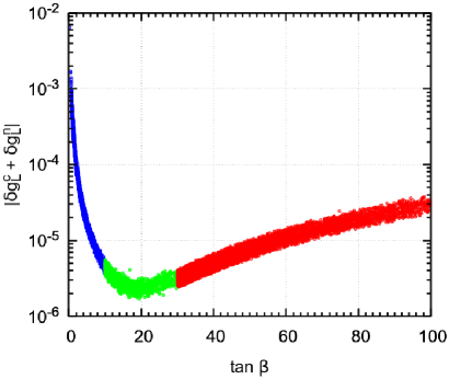
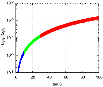
Figure 11: Total contribution of the neutral and charged scalars to $\delta g_{Lb}$ and $\delta g_{Rb}$.

We see that a significant impact on $A_{b}$ and $R_{b}$ can only occur for either very low or very high values of $\tan\beta$; namely, for $\tan{\beta}\lesssim 1$, $\delta g_{Lb}^{c}+\delta g_{Lb}^{n}\sim 10^{-3}$, and for $\tan{\beta}\gtrsim 50$, $-\delta g_{Rb}^{c}-\delta g_{Rb}^{n}\gtrsim 10^{-3}$.

Both Figs. 10 and 11 are depicted together in Fig. 12.

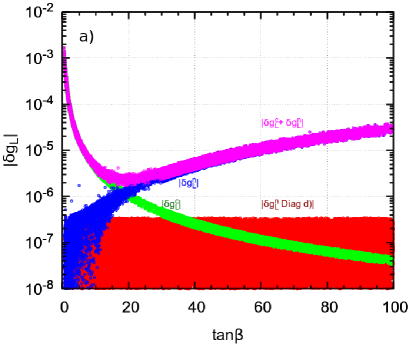
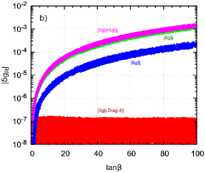
Figure 12: Left panel: comparison of the neutral-scalars contribution $\delta g_{Lb}^{n}$ (in blue) and of the charged-scalar contribution $\delta g_{Lb}^{c}$ (in green) with $\delta g_{Lb}=\delta g_{Lb}^{n}+\delta g_{Lb}^{c}$ (in pink). Right panel: comparison of the neutral-scalars contribution $\delta g_{Rb}^{n}$ (in blue) and of the charged-scalar contribution $\delta g_{Rb}^{c}$ (in green) with $\delta g_{Rb}=\delta g_{Rb}^{n}+\delta g_{Rb}^{c}$ (in pink). Also displayed (in red) are the contributions of the diagrams in Fig. 3c),d) to both $\delta g_{Lb}^{n}$ (in the left panel) and $\delta g_{Rb}^{n}$ (in the right panel).

In particular, in Fig. 12a) we see that the neutral-scalar contribution to $\delta g_{Lb}$ becomes larger than the charged-scalar contribution, eventually by many orders of magnitude, as soon as $\tan{\beta}>30$. Thus, one cannot neglect the contribution of the neutral scalars to $\delta g_{Lb}$. We expect this effect to be even more important in models with more than two Higgs doublets and/or extra singlets.

It is interesting to inquire about the importance of the type d) neutral-scalar contributions (red in Fig. 12). One sees that, when $\tan{\beta}$ is low, they may constitute a substantial part of the $\delta g_{\aleph b}^{n}$ ($\aleph=L,R$), but that is precisely the range when the $\delta g_{\aleph b}^{n}$ are anyway much too small to be of practical relevance. We conclude that, at least in this particular case, it is correct to neglect the diagrams in Fig. 3c),d), as was done in Ref. [7].

The impact on $A_{b}$ and $R_{b}$ is shown in Fig. 13 for all values of $\tan\beta$ and including the various contributions.

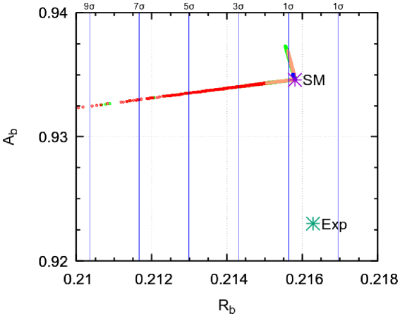
Figure 13: $A_{b}$ versus $R_{b}$ in the C2HDM for all values of $0<\tan\beta<100$. The charged-scalar contribution is shown in red for low $\tan{\beta}$ and in orange for large $\tan{\beta}$. The contribution of the neutral-scalars is in blue and lies very close to the SM point. In green (in background) the sum of the contributions.

In the low $\tan\beta$ regime, the charged-scalar contribution (shown in red) is dominant. The points in Fig. 13 only stray from the 2$\sigma$ $R_{b}$ bounds for $\tan{\beta}<0.8$. This is the reason why only points with $\tan{\beta}>0.8$ were taken in Ref. [44]. In orange is shown the contribution of the charged scalars for $\tan{\beta}$ up to 100. The contribution of the neutral scalars is in blue, and is always very small. We have verified that for the neutral scalars to have meaningful impact, one would have to consider values of $\tan\beta>250$, which would violate perturbativity of the Yukawa couplings.

We conclude that, when studying the impact on $Z\rightarrow b\bar{b}$ of multi-scalar models with very large couplings (which means very large $\tan{\beta}$ in our example of the C2HDM), the neutral scalar contributions should be taken into account. Of course, in studying any model one needs to include all the theoretical and experimental constraints, and this may curtail a large part of the phase space for such extreme couplings. This will have to be evaluated in a case by case basis.

6 Conclusions

We have studied the one-loop contributions to $Z\rightarrow b\bar{b}$ in models with extra scalars. We have started by deriving the conditions on generic couplings that must hold for the divergences to cancel. We have then concentrated on models with any number of extra $SU(2)_{L}$ doublets and singlets, either neutral, as in Ref. [7], or charged. The final expressions are greatly simplified (and very compact), due to the parameterization in Refs. [25, 26, 27, 28]. We also extend the analysis in Ref. [7] to models with CP violation in the scalar sector. We have shown that, in these general models, the conditions previously derived necessary for the cancellation of the divergences naturally hold. We have then highlighted the possible importance of the neutral-scalar contributions. In particular, in Fig. 7 and Fig. 12a) we show that, in a specific models, the contributions of the neutral scalars to $\delta g_{Lb}$ may in some cases be much larger than the contributions of the charged scalars, and this has to be considered in evaluating the limits on $A_{b}$ and $R_{b}$ as shown, for instance, in Fig. 9.

Appendix A Passarino–Veltman functions

In this appendix we expose our definition of the Passarino–Veltman functions, which coincides with that of FeynCalc [33, 34] and LoopTools [37, 38] used in the algebraic and numerical calculations [35]. We use dimensional regularization; the Feynman integrals are performed in a space–time of dimension $d=4-\epsilon$. Then,

$$\mu^{\epsilon}\!\int\!\frac{\mathrm{d}^{d}k}{\left(2\pi\right)^{d}}\ \frac{1}{k^{2}-m_{0}^{2}}\ \frac{1}{\left(k+r\right)^{2}-m_{1}^{2}}\ k^{\lambda}=\frac{i}{16\pi^{2}}\ r^{\lambda}\,B_{1}\left(r^{2},m_{0}^{2},m_{1}^{2}\right).$$ (113)

Moreover,

$$\mu^{\epsilon}\!\int\!\frac{\mathrm{d}^{d}k}{\left(2\pi\right)^{d}}\ \frac{1}{k^{2}-m_{0}^{2}}\ \frac{1}{\left(k+r_{1}\right)^{2}-m_{1}^{2}}\ \frac{1}{\left(k+r_{2}\right)^{2}-m_{2}^{2}}$$ (114)

$$= \frac{i}{16\pi^{2}}\ C_{0}\left[r_{1}^{2},\left(r_{1}-r_{2}\right)^{2},r_{2}^{2},m_{0}^{2},m_{1}^{2},m_{2}^{2}\right].$$

Also,

$$\mu^{\epsilon}\!\int\!\frac{\mathrm{d}^{d}k}{\left(2\pi\right)^{d}}\ \frac{1}{k^{2}-m_{0}^{2}}\ \frac{1}{\left(k+r_{1}\right)^{2}-m_{1}^{2}}\ \frac{1}{\left(k+r_{2}\right)^{2}-m_{2}^{2}}\ k^{\lambda}$$ (115)

$$= \frac{i}{16\pi^{2}}\left(r_{1}^{\lambda}\,C_{1}+r_{2}^{\lambda}\,C_{2}\right)\left[r_{1}^{2},\left(r_{1}-r_{2}\right)^{2},r_{2}^{2},m_{0}^{2},m_{1}^{2},m_{2}^{2}\right].$$

Finally,

$$\mu^{\epsilon}\!\int\!\frac{\mathrm{d}^{d}k}{\left(2\pi\right)^{d}}\ \frac{1}{k^{2}-m_{0}^{2}}\ \frac{1}{\left(k+r_{1}\right)^{2}-m_{1}^{2}}\ \frac{1}{\left(k+r_{2}\right)^{2}-m_{2}^{2}}\ \!k^{\lambda}k^{\nu}$$ (116)

$$= \frac{i}{16\pi^{2}}\left[g^{\lambda\nu}C_{00}+r_{1}^{\lambda}r_{1}^{\nu}C_{11}+r_{2}^{\lambda}r_{2}^{\nu}C_{22}\right.$$

$$\left.+\left(r_{1}^{\lambda}r_{2}^{\nu}+r_{2}^{\lambda}r_{1}^{\nu}\right)C_{12}\right]\left[r_{1}^{2},\left(r_{1}-r_{2}\right)^{2},r_{2}^{2},m_{0}^{2},m_{1}^{2},m_{2}^{2}\right].$$

References

- [1] ATLAS, G. Aad et al., Phys. Lett. B 716, 1 (2012), [1207.7214].
- [2] CMS, S. Chatrchyan et al., Phys. Lett. B 716, 30 (2012), [1207.7235].
- [3] J. F. Gunion, H. E. Haber, G. L. Kane and S. Dawson, The Higgs hunter’s guide (Westview Press, 1990), Frontiers in Physics.
- [4] G. C. Branco et al., Phys. Rept. 516, 1 (2012), [1106.0034].
- [5] I. P. Ivanov, Prog. Part. Nucl. Phys. 95, 160 (2017), [1702.03776].
- [6] J. C. Romao and J. P. Silva, Int. J. Mod. Phys. A27, 1230025 (2012), [1209.6213].
- [7] H. E. Haber and H. E. Logan, Phys. Rev. D62, 015011 (2000), [hep-ph/9909335].
- [8] Particle Data Group, M. Tanabashi et al., Phys. Rev. D98, 030001 (2018).
- [9] G. Dorsch, S. Huber and J. No, JHEP 10, 029 (2013), [1305.6610].
- [10] P. Basler, M. Krause, M. Mühlleitner, J. Wittbrodt, and A. Wlotzka, JHEP 02, 121 (2017), [1612.04086].
- [11] M. Krause, M. Mühlleitner, R. Santos, and H. Ziesche, Phys. Rev. D 95, 075019 (2017), [1609.04185].
- [12] D. Fontes, J. C. Romão, J. P. Silva, and R. Santos, Large pseudo-scalar components in the C2HDM, in 2nd Toyama International Workshop on Higgs as a Probe of New Physics (HPNP2015) Toyama, Japan, February 11-15, 2015, 2015, [1506.00860].
- [13] W. Mader, J.-H. Park, G. M. Pruna, D. Stöckinger, and A. Straessner, JHEP 09, 125 (2012), [1205.2692], [Erratum: JHEP 01, 006 (2014)].
- [14] H. Bélusca-Maïto, A. Falkowski, D. Fontes, J. C. Romão and J. P. Silva, Eur. Phys. J. C 77, 176 (2017), [1611.01112].
- [15] R. Campbell, S. Godfrey, H. E. Logan and A. Poulin, Phys. Rev. D 95, 016005 (2017), [1610.08097].
- [16] K. Hartling, K. Kumar and H. E. Logan, Phys. Rev. D 91, 015013 (2015), [1410.5538].
- [17] K. Hartling, K. Kumar and H. E. Logan, Phys. Rev. D 90, 015007 (2014), [1404.2640].
- [18] C.-W. Chiang, S. Kanemura and K. Yagyu, Phys. Rev. D 90, 115025 (2014), [1407.5053].
- [19] C. Degrande, K. Hartling, H. E. Logan, A. D. Peterson and M. Zaro, Phys. Rev. D 93, 035004 (2016), [1512.01243].
- [20] Y.-L. Tang, Phys. Rev. D 97, 035020 (2018), [1709.07735].
- [21] S. von Buddenbrock et al., J. Phys. G 46, 115001 (2019), [1809.06344].
- [22] L. Wang, R. Shi and X.-F. Han, Phys. Rev. D 96, 115025 (2017), [1708.06882].
- [23] H. Flächer et al., Eur. Phys. J. C 60, 543 (2009), [0811.0009], [Erratum: Eur.Phys.J.C 71, 1718 (2011)].
- [24] J. Haller et al., Eur. Phys. J. C 78, 675 (2018), [1803.01853].
- [25] W. Grimus and L. Lavoura, Phys. Rev. D 66, 014016 (2002), [hep-ph/0204070].
- [26] W. Grimus, L. Lavoura, O. M. Ogreid and P. Osland, J. Phys. G35, 075001 (2008), [0711.4022].
- [27] W. Grimus, L. Lavoura, O. Ogreid and P. Osland, Nucl. Phys. B 801, 81 (2008), [0802.4353].
- [28] W. Grimus and H. Neufeld, Nucl. Phys. B 325, 18 (1989).
- [29] W. F. L. Hollik, Fortsch. Phys. 38, 165 (1990).
- [30] W. Hollik, Adv. Ser. Direct. High Energy Phys. 14, 37 (1995).
- [31] N. D. Christensen and C. Duhr, Comput.Phys.Commun. 180, 1614 (2009), [0806.4194].
- [32] P. Nogueira, J. Comput. Phys. 105, 279 (1993).
- [33] R. Mertig, M. Böhm, and A. Denner, Comput. Phys. Commun. 64, 345 (1991), Available at https://www.feyncalc.org/.
- [34] V. Shtabovenko, R. Mertig and F. Orellana, Comput. Phys. Commun. 207, 432 (2016), [1601.01167].
- [35] D. Fontes and J. C. Romão, Comput. Phys. Commun. (2020), [1909.05876].
- [36] G. Passarino and M. J. G. Veltman, Nucl. Phys. B160, 151 (1979).
- [37] T. Hahn and M. Perez-Victoria, Comput. Phys. Commun. 118, 153 (1999), [hep-ph/9807565].
- [38] G. van Oldenborgh, Comput. Phys. Commun. 66, 1 (1991).
- [39] A. Kundu and B. Mukhopadhyaya, Int. J. Mod. Phys. A11, 5221 (1996), [hep-ph/9507305].
- [40] J. Field, Mod. Phys. Lett. A 13, 1937 (1998), [hep-ph/9801355].
- [41] J. F. Gunion and H. E. Haber, Phys. Rev. D 67, 075019 (2003), [hep-ph/0207010].
- [42] F. Botella and J. P. Silva, Phys. Rev. D 51, 3870 (1995), [hep-ph/9411288].
- [43] A. W. El Kaffas, P. Osland and O. M. Ogreid, Nonlin. Phenom. Complex Syst. 10, 347 (2007), [hep-ph/0702097].
- [44] D. Fontes et al., JHEP 02, 073 (2018), [1711.09419].
- [45] A. Djouadi, J. Kalinowski and M. Spira, Comput. Phys. Commun. 108, 56 (1998), [hep-ph/9704448].
- [46] A. Djouadi, J. Kalinowski, M. Muehlleitner and M. Spira, Comput. Phys. Commun. 238, 214 (2019), [1801.09506].
- [47] O. Deschamps et al., Phys. Rev. D 82, 073012 (2010), [0907.5135].
- [48] F. Mahmoudi and O. Stal, Phys. Rev. D 81, 035016 (2010), [0907.1791].
- [49] M. Misiak and M. Steinhauser, Eur. Phys. J. C 77, 201 (2017), [1702.04571].
- [50] F. Mahmoudi, PoS CHARGED2016, 012 (2017).
- [51] S. Kanemura, T. Kubota and E. Takasugi, Phys. Lett. B 313, 155 (1993), [hep-ph/9303263].
- [52] I. Ginzburg and I. Ivanov, Phys. Rev. D 72, 115010 (2005), [hep-ph/0508020].
- [53] D. Fontes, J. C. Romão and J. P. Silva, Phys. Rev. D90, 015021 (2014), [1406.6080].