Short-distance constraints on hadronic light-by-light scattering
in the anomalous magnetic moment of the muon

Abstract

A key ingredient in the evaluation of hadronic light-by-light (HLbL) scattering in the anomalous magnetic moment of the muon $(g-2)_{\mu}$ concerns short-distance constraints that follow from QCD by means of the operator product expansion. Here we concentrate on the most important such constraint, in the longitudinal amplitudes, and show that it can be implemented efficiently in terms of a Regge sum over excited pseudoscalar states, constrained by phenomenological input on masses, two-photon couplings, as well as short-distance constraints on HLbL scattering and the pseudoscalar transition form factors. Our estimate of the effect of the longitudinal short-distance constraints on the HLbL contribution is: $\Delta a_{\mu}^{\text{LSDC}}=13(6)\times 10^{-11}$. This is significantly smaller than previous estimates, which mostly relied on an ad-hoc modification of the pseudoscalar poles and led to up to a $40\%$ increase with respect to the nominal pseudoscalar-pole contributions, when evaluated with modern input for the relevant transition form factors. We also comment on the status of the transversal short-distance constraints and, by matching to perturbative QCD, argue that the corresponding correction will be significantly smaller than its longitudinal counterpart.

I Introduction

The precision of the Standard-Model (SM) prediction for the anomalous magnetic moment of the muon, $a_{\mu}=(g-2)_{\mu}/2$, is limited by hadronic contributions. Already at the level of the current experiment Bennett et al. (2006)

$$a_{\mu}^{\text{exp}}=116\ 592\ 089(63)\times 10^{-11},$$ (1)

estimates of the hadronic effects are crucial in evaluating the significance of the tension with the SM value, at the level of $3.5\,\sigma$. With the forthcoming Fermilab E989 experiment Grange et al. (2015), promising an improvement by a factor of $4$, as well as the E34 experiment at J-PARC Abe et al. (2019), the SM model evaluation needs to follow suit.

To this end, the relevant matrix elements need to be calculated either directly from QCD or be constrained by experimental data. The latter approach has traditionally been followed for hadronic vacuum polarization (HVP), which requires the two-point function of two electromagnetic currents and can be reconstructed from the cross section of $e^{+}e^{-}\to\text{hadrons}$ Keshavarzi et al. (2018); Jegerlehner (2019); Colangelo et al. (2019a); Hoferichter et al. (2019); Davier et al. (2019). More recently, evaluations in lattice QCD have made significant progress Borsanyi et al. (2018); Blum et al. (2018); Giusti et al. (2018); Shintani and Kuramashi (2019); Davies et al. (2020); Gérardin et al. (2019a); Aubin et al. (2020), but are not yet at the level of the data-driven, dispersive approach.

Next to HVP, the second-largest contribution to the uncertainty arises from hadronic light-by-light scattering. While also in this case progress in lattice QCD is promising Blum et al. (2017a, b); Asmussen et al. (2019), another key development in recent years concerns the phenomenological evaluation, i.e., the use of dispersion relations to remove the reliance on hadronic models, either directly for the required four-point function that defines the HLbL tensor Hoferichter et al. (2014a); Colangelo et al. (2014a, b); Colangelo et al. (2015); Colangelo et al. (2017a, b), the Pauli form factor Pauk and Vanderhaeghen (2014), or in terms of sum rules Pascalutsa et al. (2012); Green et al. (2015); Danilkin and Vanderhaeghen (2017); Hagelstein and Pascalutsa (2018, 2019). In particular, organizing the calculation in terms of dispersion relations for the HLbL tensor has led to a solid understanding of the contributions related to the lowest-lying singularities—the single-particle poles from $P=\pi^{0},\eta,\eta^{\prime}$ and cuts from two-pion intermediate states—largely because the hadronic quantities determining the strength of these singularities, the $P\to\gamma^{*}\gamma^{*}$ transition form factors Hoferichter et al. (2014b); Masjuan and Sanchez-Puertas (2017); Hoferichter et al. (2018a, b); Gérardin et al. (2019b); Eichmann et al. (2019) and the helicity amplitudes for $\gamma^{*}\gamma^{*}\to\pi\pi$ García-Martín and Moussallam (2010); Hoferichter et al. (2011); Moussallam (2013); Danilkin and Vanderhaeghen (2019); Hoferichter and Stoffer (2019); Danilkin et al. (2020), respectively, can be provided as external input quantities, in a similar spirit as the $e^{+}e^{-}\to\text{hadrons}$ cross section for HVP. Higher-order iterations of HVP Calmet et al. (1976); Keshavarzi et al. (2018); Kurz et al. (2014) and HLbL Colangelo et al. (2014c) are already sufficiently under control.

For both HVP and HLbL, data-driven evaluations of the hadronic corrections to $(g-2)_{\mu}$ are fundamentally limited by the fact that experimental input is only available in a given energy range, so that the tails of the dispersion integrals have to be estimated by other means, most notably short-distance constraints as derived from perturbative QCD (pQCD). In addition, even for HVP, short-distance constraints have been used for energies as low as $2\,\text{GeV}$ as a supplement to (and check of) experiment, with good agreement found between the pQCD prediction and data in between resonances Keshavarzi et al. (2018); Davier et al. (2019). For HLbL scattering such constraints become even more important given the limited information on the HLbL tensor for intermediate and high energies.

Two kinematic configurations are relevant for the HLbL contribution, one in which all photon virtualities $Q_{i}^{2}$ are large, and a second in which one of the non-vanishing virtualities remains small compared to the others $Q_{3}^{2}\ll Q_{1}^{2}\sim Q_{2}^{2}$. Recently, it was shown that the former situation can be addressed in a systematic operator product expansion (OPE), in which the pQCD quark loop emerges as the first term in the expansion Bijnens et al. (2019). The second configuration is related to so-called mixed regions in the $g-2$ integral, i.e., integration regions in which asymptotic arguments only apply to a subset of the kinematic variables, while hadronic physics may still be relevant for others. A key insight derived in Melnikov and Vainshtein (2004) was that such effects can also be constrained with an OPE, by reducing the HLbL tensor to a vector–vector–axial-vector ($VVA$) three-point function and using known results for the corresponding anomaly and its (non-) renormalization Vainshtein (2003); Knecht et al. (2004, 2002a); Czarnecki et al. (2003); Jegerlehner and Tarasov (2006); Mondejar and Melnikov (2013). The explicit implementation suggested in Melnikov and Vainshtein (2004) relied on the observation that both the OPE constraint and the normalization are satisfied if the momentum dependence of the singly-virtual form factor describing the pseudoscalar-pole contribution is neglected. However, such a modification is not compatible with a description based on dispersion relations for the HLbL tensor.

Here, we suggest to implement the corresponding longitudinal short-distance constraints in terms of excited pseudoscalar states. As we will show, not only can the asymptotic limits be implemented in a fairly economical manner, but the critical mixed regions can be constrained by phenomenological input for the masses and two-photon couplings of the lowest pseudoscalar excitations. The model dependence can be further reduced by matching to the pQCD quark loop, which, in addition, allows one to gain some insights into the scale where hadronic and pQCD-based descriptions should meet.

II OPE constraints on HLbL scattering

The HLbL tensor is defined as the four-point function

$$\Pi^{\mu\nu\lambda\sigma}(q_{1},q_{2},q_{3}) =-i\int d^{4}x\,d^{4}y\,d^{4}z\,e^{-i(q_{1}\cdot x+q_{2}\cdot y+q_{3}\cdot z)}$$

$$\times\langle 0|T\{j_{\text{em}}^{\mu}(x)j_{\text{em}}^{\nu}(y)j_{\text{em}}^{\lambda}(z)j_{\text{em}}^{\sigma}(0)\}|0\rangle$$ (2)

of four electromagnetic currents

$$j_{\text{em}}^{\mu}=\bar{q}\mathcal{Q}\gamma^{\mu}q,\quad\mathcal{Q}=\text{diag}\left(\frac{2}{3},-\frac{1}{3},-\frac{1}{3}\right),$$ (3)

where $q_{i}$ denote the photon virtualities, $q_{4}=q_{1}+q_{2}+q_{3}$, and $q=(u,d,s)^{T}$ the quark fields. We work with the decomposition into scalar functions $\Pi_{i}$,

$$\Pi^{\mu\nu\lambda\sigma}=\sum_{i=1}^{54}T_{i}^{\mu\nu\lambda\sigma}\Pi_{i},$$ (4)

derived in Colangelo et al. (2015); Colangelo et al. (2017b) following the general principle established by Bardeen, Tung Bardeen and Tung (1968), and Tarrach Tarrach (1975) (BTT). The contribution to $(g-2)_{\mu}$ then follows via

$$a_{\mu}^{\mathrm{HLbL}} =\frac{2\alpha^{3}}{3\pi^{2}}\int_{0}^{\infty}dQ_{1}\int_{0}^{\infty}dQ_{2}\int_{-1}^{1}d\tau\sqrt{1-\tau^{2}}\,Q_{1}^{3}Q_{2}^{3}$$

$$\times\sum_{i=1}^{12}T_{i}(Q_{1},Q_{2},\tau)\bar{\Pi}_{i}(Q_{1},Q_{2},Q_{3}),$$ (5)

where $Q_{i}^{2}=-q_{i}^{2}$ are the Wick-rotated virtualities, $Q_{3}^{2}=Q_{1}^{2}+Q_{2}^{2}+2Q_{1}Q_{2}\tau$, the $\bar{\Pi}_{i}$ refer to certain linear combinations of $\Pi_{i}$, and the $T_{i}$ are known kernel functions Colangelo et al. (2015); Colangelo et al. (2017b).

In the limit where all $Q_{i}^{2}$ are large, the calculation from Bijnens et al. (2019) proves the earlier statement of Melnikov and Vainshtein (2004) that the pQCD quark loop arises as the first term in a systematic OPE. In particular, this implies the constraint

$$\lim_{Q\to\infty}Q^{4}\,\bar{\Pi}_{1}(Q,Q,Q)=-\frac{4}{9\pi^{2}}.$$ (6)

The second kinematic configuration Melnikov and Vainshtein (2004), $Q^{2}\equiv Q_{1}^{2}\sim Q_{2}^{2}\gg Q_{3}^{2}$, when expressed in BTT basis, leads to the constraint

$$\lim_{Q_{3}\to\infty}\lim_{Q\to\infty}Q^{2}Q_{3}^{2}\,\bar{\Pi}_{1}(Q,Q,Q_{3})=-\frac{2}{3\pi^{2}}.$$ (7)

The latter result can be derived by considering the $VVA$ triangle anomaly and its non-renormalization theorems Vainshtein (2003); Knecht et al. (2004, 2002a); Czarnecki et al. (2003); Jegerlehner and Tarasov (2006); Mondejar and Melnikov (2013). Its constraint on $\bar{\Pi}_{1}$ (and, by crossing symmetry, $\bar{\Pi}_{2}$) corresponds to the longitudinal amplitudes in the $VVA$ matrix element and we will therefore refer to $\bar{\Pi}_{1,2}$ as the longitudinal amplitudes and, accordingly, their constraints as longitudinal short-distance constraints. Further, the limit (7) is intimately related to the pseudoscalar poles

$$\bar{\Pi}_{1}^{P\text{-pole}}=\frac{F_{P\gamma^{*}\gamma^{*}}(q_{1}^{2},q_{2}^{2})F_{P\gamma\gamma^{*}}(q_{3}^{2})}{q_{3}^{2}-M_{P}^{2}},$$ (8)

where $P=\pi^{0},\eta,\eta^{\prime}$, and the doubly-virtual $F_{P\gamma^{*}\gamma^{*}}(q_{1}^{2},q_{2}^{2})$ and singly-virtual $F_{P\gamma\gamma^{*}}(q_{3}^{2})$ transition form factors determine the residue of the poles. They are subject to short-distance constraints themselves, for the pion we have the asymptotic constraint Novikov et al. (1984)

$$\lim_{Q^{2}\rightarrow\infty}Q^{2}F_{\pi^{0}\gamma^{*}\gamma^{*}}(-Q^{2},-Q^{2})=\frac{2F_{\pi}}{3},$$ (9)

as well as the Brodsky–Lepage limit Lepage and Brodsky (1979, 1980); Brodsky and Lepage (1981)

$$\lim_{Q^{2}\rightarrow\infty}Q^{2}F_{\pi^{0}\gamma\gamma^{*}}(-Q^{2})=2F_{\pi}.$$ (10)

Together with the normalization

$$F_{\pi^{0}\gamma\gamma}=\frac{1}{4\pi^{2}F_{\pi}},$$ (11)

the former shows that if $F_{\pi^{0}\gamma\gamma^{*}}(q_{3}^{2})\to F_{\pi^{0}\gamma\gamma}$ in (8), the pion decay constant $F_{\pi}$ would drop out and the pion would account for $-1/(6\pi^{2})$ in (7). Similarly, $\eta$ and $\eta^{\prime}$ would provide the remaining $-1/(2\pi^{2})$. This is the essence of the model suggested in Melnikov and Vainshtein (2004, 2019).

However, a constant singly-virtual transition form factor cannot be justified within a dispersive approach for general HLbL scattering. Instead, one would need to consider dispersion relations in the photon virtualities $q_{i}^{2}$ already in reduced $g-2$ kinematics, and even then the residue would involve $F_{\pi^{0}\gamma\gamma^{*}}(M_{P}^{2})$, not the normalization itself. Further, when writing dispersion relations in the $q_{i}^{2}$ for $g-2$ kinematics, there is no clear separation between the singularities of the HLbL amplitude and those generated by hadronic intermediate states directly coupling to individual electromagnetic currents, such as $2\pi$ states. In the dispersive approach for general HLbL scattering the latter appear only in the transition form factors, which factor out and can be treated as external input quantities. In this sense, neglecting the momentum dependence of the singly-virtual transition form factor without at the same time accounting for the additional cuts, leads to a distortion of the low-energy properties of the HLbL tensor.

Instead, we propose here a solution based on a remark already made in Melnikov and Vainshtein (2004): while a finite number of pseudoscalar poles, due to (11), cannot fulfill the OPE constraint (7), an infinite series potentially can. The basic idea can be illustrated for large-$N_{c}$ Regge models of the transition form factor itself Ruiz Arriola and Broniowski (2006); Ruiz Arriola and Broniowski (2010), which assume a radial Regge trajectory to describe the masses of excited vector mesons,

$$M_{V(n)}^{2}=M_{V}^{2}+n\,\sigma_{V}^{2},$$ (12)

and rely on the ansatz:

$$F_{P\gamma^{*}\gamma^{*}}(-Q^{2},-Q^{2})\propto\sum_{n=0}^{\infty}\,\frac{1}{[Q^{2}+M_{V(n)}^{2}]^{2}}$$

$$=\frac{1}{\sigma_{V}^{4}}\,\psi^{(1)}\left(\frac{M_{V}^{2}+Q^{2}}{\sigma_{V}^{2}}\right)\sim\frac{1}{Q^{2}},$$ (13)

with $\psi^{(1)}$ the trigamma function and the Regge slope $\sigma_{V}$. In this way, the infinite sum produces the correct asymptotic behavior (10), even though none of the individual terms do.

One may wonder about the fate of the infinite sum over excited pseudoscalar states in the chiral limit, given that their decay constants are expected to vanish with the quark masses. We show below how the matching to pQCD removes the model dependence regarding which states are used to satisfy the short-distance constraints, so that the implementation in terms of pseudoscalar excitations mainly adds an estimate for the mixed-region contribution, driven by the phenomenology of the lowest excitations as well as the respective short-distance constraints.

III Large-$\boldsymbol{N_{c}}$ Regge model

In the following, we present a large-$N_{c}$-inspired Regge model in the pseudoscalar and vector-meson sectors of QCD that allows us to satisfy the short-distance constraints via an infinite sum of pseudoscalar-pole diagrams (see, e.g., Peris et al. (1998); Knecht et al. (1998); Bijnens et al. (2003) for the use of large-$N_{c}$ arguments to simultaneously fulfill low- and high-energy constraints). For brevity, we focus our description on the pion, referring for a complete and more detailed account to Colangelo et al. (2019b). We start from a standard large-$N_{c}$ ansatz for the pion transition form factors as in (13), but differentiate between $\rho$ and $\omega$ trajectories, which are assumed to enter with diagonal couplings due to the wave function overlap Ruiz Arriola and Broniowski (2006); Ruiz Arriola and Broniowski (2010). In a first step, we seek an extension of this model that satisfies the constraints (9)–(11) for the transition form factor as well as (6) and (7) for the HLbL tensor

$$F_{\pi(n)\gamma^{*}\gamma^{*}}(-Q_{1}^{2},-Q_{2}^{2})$$

$$=\frac{1}{8\pi^{2}F_{\pi}}\left\{\left(\frac{M_{\rho}^{2}M_{\omega}^{2}}{D_{\rho(n)}^{1}D_{\omega(n)}^{2}}+\frac{M_{\rho}^{2}M_{\omega}^{2}}{D_{\rho(n)}^{2}D_{\omega(n)}^{1}}\right)\Bigg{[}c_{\mathrm{anom}}\right.$$

$$+\left.\frac{1}{\Lambda^{2}}\left(c_{A}M_{+,\,n}^{2}+c_{B}M_{-,\,n}^{2}\right)+c_{\mathrm{diag}}\frac{Q_{1}^{2}Q_{2}^{2}}{\Lambda^{2}(Q_{+}^{2}+M^{2}_{\mathrm{diag}})}\right]$$

$$+\frac{Q_{-}^{2}}{Q_{+}^{2}}\left[c_{\mathrm{BL}}+\frac{1}{\Lambda^{2}}\left(c_{A}M_{-,\,n}^{2}+c_{B}M_{+,\,n}^{2}\right)\right]$$

$$\times\left.\left(\frac{M_{\rho}^{2}M_{\omega}^{2}}{D_{\rho(n)}^{1}D_{\omega(n)}^{2}}-\frac{M_{\rho}^{2}M_{\omega}^{2}}{D_{\rho(n)}^{2}D_{\omega(n)}^{1}}\right)\right\},$$ (14)

where $Q_{\pm}^{2}=Q_{1}^{2}\pm Q_{2}^{2}$, $M_{\pm,\,n}^{2}=\frac{1}{2}[M_{\omega(n)}^{2}\pm M_{\rho(n)}^{2}]$, $D^{i}_{X}=Q_{i}^{2}+M_{X}^{2}$, and $\Lambda=\mathcal{O}(1\,\text{GeV})$ a typical QCD scale. The five dimensionless parameters $c_{\mathrm{anom}}$, $c_{A}$, $c_{B}$, $c_{\mathrm{diag}}$, $c_{\mathrm{BL}}$ are used to fulfill all the constraints, while the remaining parameter $M_{\mathrm{diag}}$ is adjusted to reproduce the ground-state $\pi^{0}$ transition form factor Hoferichter et al. (2018a, b). In the minimal model (14), we only allow $\pi(n)$ to couple to $\rho(n)$ and $\omega(n)$, i.e., the couplings are fully diagonal in the excitation numbers, while the effect of the eliminated vector-meson excitations is subsumed into a $Q_{i}^{2}$ dependence of the numerator multiplying the resonance propagators. In addition, we also considered an untruncated large-$N_{c}$ model, in which both the Regge summation in the transition form factor itself (13) and the HLbL tensor are retained, to assess the systematics in the large-$N_{c}$ ansatz Colangelo et al. (2019b). Using the Regge slopes from Masjuan et al. (2012) and the other input parameters from Tanabashi et al. (2018), we find that we can indeed reproduce well the $\pi^{0}$ transition form factor, which also ensures that effective-field-theory constraints on the pion-pole contribution to $(g-2)_{\mu}$ Knecht et al. (2002b); Ramsey-Musolf and Wise (2002) are fulfilled Hoferichter et al. (2018b). Finally, the model predicts a two-photon coupling of the first excited pion, $\pi(1300)$, in line with its phenomenological bound $F_{\pi(1300)\gamma\gamma}<0.0544(71)\,\text{GeV}^{-1}$ Acciarri et al. (1997); Salvini et al. (2004).

Constructing a large-$N_{c}$ Regge model for $\eta^{(\prime)}$ proceeds along the same lines, but involves several complications. First, the $\rho$ and $\omega$ trajectories do not suffice to incorporate all constraints since due to the $I=0$ nature of $\eta^{(\prime)}$ only equal-mass combinations of vector mesons ($2\rho$, $2\omega$, $2\phi$) contribute to (14), so that only three model parameters survive. To provide sufficient freedom in satisfying all constraints the consideration of $\omega$–$\phi$ mixing cannot be avoided. In addition, $\eta$–$\eta^{\prime}$ mixing needs to be taken into account, both for the flavor decomposition of the short-distance constraints as well as the relative weights of the vector-meson combinations in the transition form factors. The former is directly constrained by data on the transition form factors Escribano et al. (2016); Masjuan and Sanchez-Puertas (2017), but for the calculation of the weights, which we extract from effective pseudoscalar–vector–vector and photon–vector Lagrangians Landsberg (1985); Meißner (1988), it is more convenient to work with the phenomenological two-angle mixing scheme from Feldmann et al. (1998); Feldmann (2000). We therefore use the latter everywhere. All variants are covered by the error analysis.

The resulting $\eta$ and $\eta^{\prime}$ transition form factors are in good agreement with experimental data in the singly-virtual Acciarri et al. (1998); Behrend et al. (1991); Gronberg et al. (1998); del Amo Sanchez et al. (2011) and doubly-virtual regions Lees et al. (2018), as well as the fit results using Canterbury approximants Masjuan and Sanchez-Puertas (2017). Furthermore, there are some phenomenological constraints on the two-photon couplings for $\eta(1295)$ Acciarri et al. (2001); Ahohe et al. (2005), $\eta(1405)$ Ahohe et al. (2005); Acciarri et al. (2001); Ablikim et al. (2018), $\eta(1475)$ Achard et al. (2007); Ablikim et al. (2018), $\eta(1760)$ Zhang et al. (2012), and $X(1835)$ Zhang et al. (2012); Ablikim et al. (2018), where $\eta(1475)$ and $\eta(1760)$ are actually seen in $\gamma\gamma$ collisions, while for the others only limits are available. The detailed comparison depends on the assignment of these states into $\eta$ and $\eta^{\prime}$ trajectories, but the predictions of our model are compatible with either the assignment from Masjuan et al. (2012); Tanabashi et al. (2018) (our main choice) or the one from Klempt and Zaitsev (2007), see Colangelo et al. (2019b).

By construction, the ground-state pseudoscalar-pole contributions to $(g-2)_{\mu}$ reproduce literature values Hoferichter et al. (2018a, b); Masjuan and Sanchez-Puertas (2017); Sanchez-Puertas (2019) within errors, while the sum over excited-pseudoscalar poles leads to the increase:

$$\Delta a_{\mu}^{\pi\text{-poles}} =2.7\,(0.4)_{\text{Model}}\,(1.2)_{\text{syst}}\times 10^{-11},$$

$$\Delta a_{\mu}^{\eta\text{-poles}} =3.4^{\,+0.9}_{\,-0.7}\big{|}_{\text{Model}}\,(0.9)_{\text{syst}}\times 10^{-11},$$

$$\Delta a_{\mu}^{\eta^{\prime}\text{-poles}} =6.5\,(1.1)_{\text{Model}}\,(1.7)_{\text{syst}}\times 10^{-11},$$ (15)

where the first error refers to the uncertainties propagated from the input parameters and the systematic error is estimated by comparison to an alternative untruncated large-$N_{c}$ Regge model Colangelo et al. (2019b). Combining all pseudoscalars, we find:

$$\Delta a_{\mu}^{\text{PS-poles}} =\Delta a_{\mu}^{\pi\text{-poles}}+\Delta a_{\mu}^{\eta\text{-poles}}+\Delta a_{\mu}^{\eta^{\prime}\text{-poles}}$$

$$=12.6^{\,+1.6}_{\,-1.5}\big{|}_{\text{Model}}\,(3.8)_{\text{syst}}\times 10^{-11}$$

$$=12.6(4.1)\times 10^{-11}.$$ (16)

This result should be contrasted with the one suggested in Melnikov and Vainshtein (2004) to satisfy the mixed-region short-distance constraint (using transition form factor models from Knecht and Nyffeler (2002)): $\Delta a_{\mu}^{\text{PS-poles}}\big{|}_{\text{MV}}=23.5\times 10^{-11}$, which would become $38\times 10^{-11}$ once updated with modern input for the transition form factors, and thus suggest an increase nearly three times as large as (16) or almost $40\%$ of the nominal pseudoscalar-pole contribution. Given that arguments following Melnikov and Vainshtein (2004) have been included in previous compilations of HLbL Prades et al. (2009), a central result of this work is that such a large increase does not occur if the short-distance constraints are implemented without compromising the low-energy properties of HLbL scattering.

IV Matching to perturbative QCD

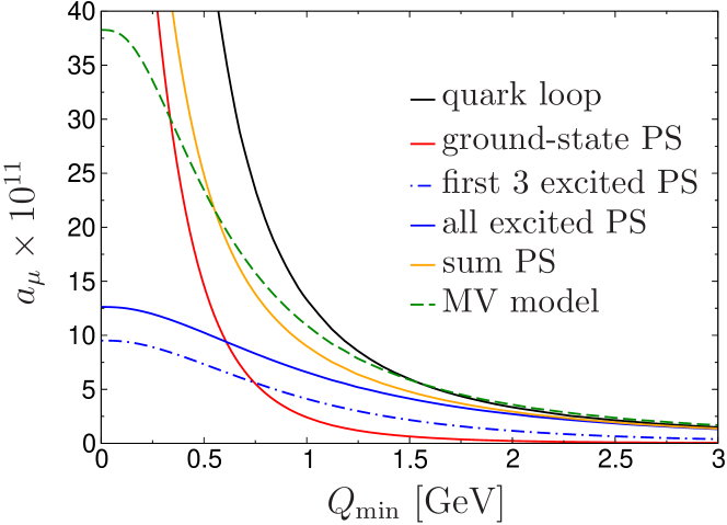
Figure 1: The longitudinal part of the massless pQCD quark loop (black), the ground-state pseudoscalars (red), the sum of all excitations from the large-$N_{c}$ Regge model (blue), the first three excitations (blue dot-dashed), the sum of ground and excited states (orange), and the increase found in the Melnikov–Vainshtein model (green dashed). The upper plot shows the contribution to $a_{\mu}$ for $Q_{i}\geq Q_{\text{min}}$, the lower for $Q_{i}\leq Q_{\text{max}}$.

Since, by construction, the sum over the pseudoscalar excitations fulfills the short-distance constraints, it has to match onto the pQCD quark loop for sufficiently large momentum transfers. In the upper plot of Fig. 1, the contribution to $(g-2)_{\mu}$ from the massless pQCD quark loop (black) and the pseudoscalar-pole contributions (sum of ground-state and excited states in orange) are compared after imposing a cutoff $Q_{\text{min}}\leq Q_{i}$ in the integration: the matching occurs somewhere around $1.5$–$2\,\text{GeV}$. The lower plot, where the opposite cutoff $Q_{\text{max}}\geq Q_{i}$ is imposed, shows that the contribution of the excited pseudoscalars (blue) to the low-energy region is very small and entirely saturated by the first few excitations (blue dot-dashed). These observations suggest to evaluate the asymptotic part of the integral $Q_{i}\geq Q_{\text{min}}$ with pQCD, to make explicit that this part of the result does not depend on the nature of hadronic states used in the implementation. Defining an optimal matching scale would require information on the uncertainty of the pQCD result. Here, we simply use a rough $20\%$ estimate, which is the size of pQCD corrections for inclusive $\tau$ decays, a process that has a similar energy scale and has been studied in detail Davier et al. (2008); Beneke and Jamin (2008); Maltman and Yavin (2008); Narison (2009); Caprini and Fischer (2009); Pich (2014).

Together with the uncertainties from the Regge model, these considerations lead to a scale $Q_{\text{match}}=1.7\,\text{GeV}$. Varying this scale within $\pm 0.5\,\text{GeV}$ and adding the systematic uncertainty from the comparison to the untruncated Regge model, we obtain as our final result:

$$\Delta a_{\mu}^{\text{LSDC}} =\left[8.7(5.5)_{\text{PS-poles}}+4.6(9)_{\text{pQCD}}\right]\times 10^{-11}$$

$$=13(6)\times 10^{-11}$$ (17)

for the increase of $(g-2)_{\mu}$ due to longitudinal short-distance constraints. In particular, the lowest three pseudoscalar excitations, whose contribution is at least partly constrained by phenomenological input on masses and two-photon couplings, give $7.8\times 10^{-11}$. Given that the most uncertain contribution, from $n>3$, thus amounts to only $10\%$ of the total, the uncertainty estimate in (17) should be conservative enough to cover the remaining model dependence. In particular, the error in (17) includes an inflation of the Regge slope uncertainties by a factor three, to allow for systematic effects that might occur if other hadronic states were used to implement the short-distance constraints. More recently, this expectation has been confirmed by models in holographic QCD based on a summation of an infinite tower of axial-vector resonances instead Leutgeb and Rebhan (2019); Cappiello et al. (2019), which despite very different assumptions and systematics yield results remarkably close to (17).

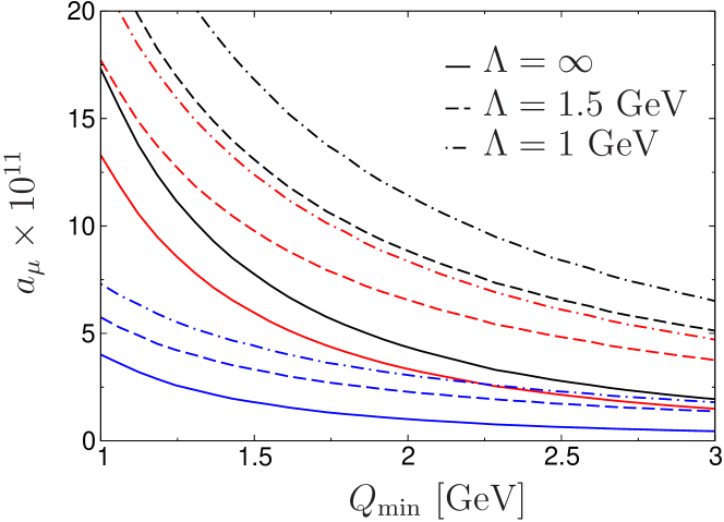
Figure 2: Contribution of the massless pQCD quark loop to $a_{\mu}$ from the region $Q_{1,2}\geq Q_{\text{min}}$, with the contribution from $Q_{3}$ below $Q_{\text{min}}$ damped by $Q_{3}^{2}/(Q_{3}^{2}+\Lambda^{2})$ (plus crossed). The total contribution (black) is split into longitudinal (red) and transversal (blue) components. The limit $Q_{i}\geq Q_{\text{min}}$ for all $Q_{i}$ is reproduced for $\Lambda\to\infty$.

With the impact of the longitudinal short-distance constraints estimated as in (17), it is natural to inquire about the role of the transversal short-distance constraints. A first estimate could again be obtained by matching to pQCD. Fig. 2 extends the integration region beyond $Q_{i}\geq Q_{\text{min}}$ into the mixed region, but suppressing this additional contribution by a factor $Q_{3}^{2}/(Q_{3}^{2}+\Lambda^{2})$, because otherwise part of the ground-state pseudoscalar contribution would be double-counted. The longitudinal result is reproduced for scales around $\Lambda\sim Q_{\text{min}}\sim 1.4\,\text{GeV}$, for which one would read off $\Delta a_{\mu}^{\text{TSDC}}\sim 4\times 10^{-11}$. Accordingly, we would expect the impact of the transversal short-distance constraints to be significantly less than that of the longitudinal ones.

We stress that the calculation presented here is complementary to higher-order calculations in pQCD and/or the OPE Bijnens et al. (2019), which would allow one to improve the matching between hadronic implementations and a perturbative description. Similarly, more experimental guidance on the two-photon couplings of hadronic states in the $1$–$2\,\text{GeV}$ region would be beneficial for the phenomenological analysis, not only for the excited pseudoscalars, but for axial-vector resonances as well, which outlines avenues for future work. We conclude that with the present analysis the biggest systematic uncertainty due to short-distance constraints has been reduced significantly, with the result that the asymptotic part of the HLbL tensor is under sufficient control for the first release from the Fermilab experiment.