Grand Unified Neutrino Spectrum at Earth:
Sources and Spectral Components

Abstract

We briefly review the dominant neutrino fluxes at Earth from different sources and present the Grand Unified Neutrino Spectrum ranging from meV to PeV energies. For each energy band and source, we discuss both theoretical expectations and experimental data. This compact review should be useful as a brief reference to those interested in neutrino astronomy, fundamental particle physics, dark-matter detection, high-energy astrophysics, geophysics, and other related topics.

I Introduction

In our epoch of multi-messenger astronomy, the Universe is no longer explored with electromagnetic radiation alone, but in addition to cosmic rays, neutrinos and gravitational waves are becoming crucial astrophysical probes. While the age of gravitational-wave detection has only begun Abbott et al. (2016), neutrino astronomy has evolved from modest beginnings in the late 1960s with first detections of atmospheric Achar et al. (1965); Reines et al. (1965) and solar neutrinos Davis et al. (1968) to a main-stream effort. Today, a vast array of experiments observes the neutrino sky over a large range of energies Koshiba (1992); Cribier et al. (1995); Becker (2008); Spiering (2012); Gaisser and Karle (2017).

When observing distant sources, inevitably one also probes the intervening space and the propagation properties of the radiation, providing tests of fundamental physics. Examples include time-of-flight limits on the masses of photons Tanabashi et al. (2018); Wei and Wu (2018); Goldhaber and Nieto (2010), gravitons Goldhaber and Nieto (2010); de Rham et al. (2017) and neutrinos Tanabashi et al. (2018); Loredo and Lamb (1989, 2002); Beacom et al. (2000); Nardi and Zuluaga (2004); Ellis et al. (2012); Lu et al. (2015), photon or graviton mixing with axion-like particles Tanabashi et al. (2018); Raffelt and Stodolsky (1988); Meyer et al. (2013, 2017); Liang et al. (2019); Galanti and Roncadelli (2018); Conlon et al. (2018), the relative propagation speed of different types of radiation Longo (1987); Stodolsky (1988); Laha (2019); Ellis et al. (2019), tests of Lorentz invariance violation Laha (2019); Ellis et al. (2019); Liberati and Maccione (2009); Liberati (2013); Guedes Lang et al. (2018), or the Shapiro time delay in gravitational potentials Longo (1988); Krauss and Tremaine (1988); Pakvasa et al. (1989); Desai and Kahya (2018); Wang et al. (2016); Shoemaker and Murase (2018); Wei et al. (2017); Boran et al. (2019).

Neutrinos are special in this regard because questions about their internal properties were on the table immediately after the first observation of solar neutrinos. The daring interpretation of the observed deficit in terms of flavor oscillations Gribov and Pontecorvo (1969), supported by atmospheric neutrino measurements Fukuda et al. (1998), eventually proved correct Aharmim et al. (2010); Esteban et al. (2017); Capozzi et al. (2018); de Salas et al. (2018). Today this effect is a standard ingredient to interpret neutrino measurements from practically any source. While some parameters of the neutrino mixing matrix remain to be settled (the mass ordering and the CP-violating phase), it is probably fair to say that in neutrino astronomy today the focus is on the sources and less on properties of the radiation. Of course, there is always room for surprises and new discoveries.

One major exception to this development is the cosmic neutrino background (CNB) that has never been directly detected and where the question of the absolute neutrino mass scale, and the Dirac vs. Majorana question, is the main unresolved issue. Here neutrinos are a hybrid between radiation and dark matter. If neutrinos were massless, the CNB today would be blackbody radiation with $T_{\nu}=1.95~{}{\rm K}=0.168~{}{\rm meV}$, whereas the minimal neutrino mass spectrum implied by flavor oscillations is $m_{1}=0$, $m_{2}=8.6$, and $m_{3}=50$ meV, but all masses could be larger in the form of a degenerate spectrum and the ordering could be inverted in the form $m_{3}<m_{1}<m_{2}$. One may actually question if future CNB measurements are part of traditional neutrino astronomy or the first case of dark-matter astronomy.

The large range of energies and the very different types of sources and detectors makes it difficult to stay abreast of the developments in the entire field of neutrino astronomy. One first entry to the subject is afforded by a graphical representation and brief explanation of what we call the Grand Unified Neutrino Spectrum (GUNS), a single plot of the neutrino and antineutrino background at Earth from the CNB in the meV range to the highest-energy cosmic neutrinos at PeV ($10^{15}~{}{\rm eV}$) energies Koshiba (1992); Haxton and Lin (2000); Cribier et al. (1995); Becker (2008); Spiering (2012); Gaisser and Karle (2017). As our main result we here produce an updated version of the GUNS plots shown in Fig. 1. The top panel shows the neutrino flux $\phi$ as a function of energy, while the energy flux $E\times\phi$ is shown in the bottom panel.

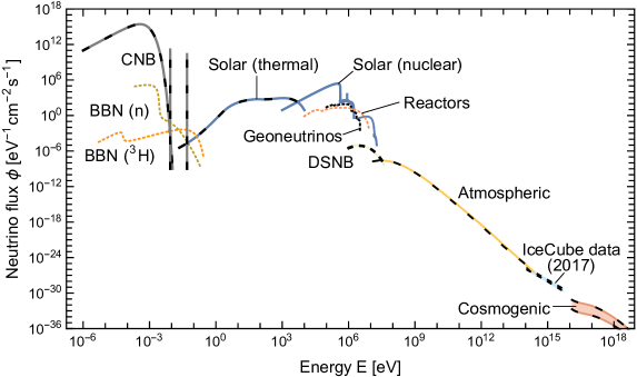
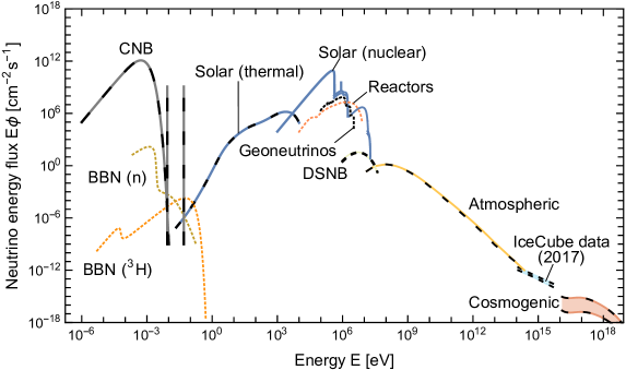
Figure 1: Grand Unified Neutrino Spectrum (GUNS) at Earth, integrated over directions and summed over flavors. Therefore, flavor conversion between source and detector does not affect this plot. Solid lines are for neutrinos, dashed or dotted lines for antineutrinos, superimposed dashed and solid lines for sources of both $\nu$ and $\overline{\nu}$. The fluxes from BBN, the Earth, and reactors encompass only antineutrinos, the Sun emits only neutrinos, whereas all other components include both. The CNB is shown for a minimal mass spectrum of $m_{1}=0$, $m_{2}=8.6$, and $m_{3}=50$ meV, producing a blackbody spectrum plus two monochromatic lines of nonrelativistic neutrinos with energies corresponding to $m_{2}$ and $m_{3}$. See Appendix D for an exact description of the individual curves. Top panel: Neutrino flux $\phi$ as a function of energy; line sources in units of ${\rm cm}^{-2}~{}{\rm s}^{-1}$. Bottom panel: Neutrino energy flux $E\times\phi$ as a function of energy; line sources in units of ${\rm eV}~{}{\rm cm}^{-2}~{}{\rm s}^{-1}$.

Our initial motivation for this task came from the low-energy part which traditionally shows a gap between solar neutrinos and the CNB, the latter usually depicted as blackbody radiation. However, the seemingly simple task of showing a new component — the keV thermal neutrino flux from the Sun and the neutrinos from $\beta$ decays of primordial elements — in the context of the full GUNS quickly turned into a much bigger project because one is forced to think about all components.

While our brief review can be minimally thought of as an updated and annotated version of the traditional GUNS plot, ideally it serves as a compact resource for students and researchers to get a first sense in particular of those parts of the spectrum where they are no immediate experts. One model for our work could be the format of the mini reviews provided in the Review of Particle Physics Tanabashi et al. (2018). In addition, we provide the input of what exactly went on the plot in the form of tables or analytic formulas (see Appendix D).

Astrophysical and terrestrial neutrino fluxes can be modified by any number of nonstandard effects, including mixing with hypothetical sterile neutrinos Mention et al. (2011); Abazajian et al. (2012), large nonstandard interactions Davidson et al. (2003); Antusch et al. (2009); Biggio et al. (2009); Ohlsson (2013), spin-flavor oscillations by large nonstandard magnetic dipole moments Raffelt (1990); Haft et al. (1994); Giunti and Studenikin (2015), decay and annihilation into majoron-like bosons Schechter and Valle (1982); Gelmini and Valle (1984); Beacom et al. (2003); Beacom and Bell (2002); Denton and Tamborra (2018b); Funcke et al. (2020); Pakvasa et al. (2013); Pagliaroli et al. (2015); Bustamante et al. (2017), for the CNB large primordial asymmetries and other novel early-universe phenomena Pastor et al. (2009); Arteaga et al. (2017), or entirely new sources such as dark-matter decay Barger et al. (2002); Halzen and Klein (2010); Fan and Reece (2013); Feldstein et al. (2013); Agashe et al. (2014); Rott et al. (2015); Kopp et al. (2015); Boucenna et al. (2015); Chianese et al. (2016); Cohen et al. (2017); Chianese et al. (2019); Esmaili and Serpico (2013); Bhattacharya et al. (2014); Higaki et al. (2014); Fong et al. (2015); Murase et al. (2015) and annihilation in the Sun or Earth Srednicki et al. (1987); Silk et al. (1985); Ritz and Seckel (1988); Kamionkowski (1991); Cirelli et al. (2005). We will usually not explore such topics and rather stay in a minimal framework which of course includes normal flavor conversion.

In the main text we walk the reader through the GUNS plots of Fig. 1 and briefly review the different components approximately in increasing order of energy. In Sec. II we begin with the CNB, discussing primarily the impact of neutrino masses. In Fig. 1 we show a minimal example where the smallest neutrino mass vanishes, providing the traditional blackbody radiation, and two mass components which are nonrelativistic today.

In Sec. III we turn to neutrinos from the big-bang nucleosynthesis (BBN) epoch that form a small but dominant contribution at energies just above the CNB. This very recently recognized flux derives from neutron and triton decays, $n\to p+e^{-}+\overline{\nu}_{e}$ and ${}^{3}{\rm H}\to{}^{3}{\rm He}+e^{-}+\overline{\nu}_{e}$, that are left over from BBN.

In Sec. IV we turn to the Sun, which is especially bright in neutrinos because of its proximity, beginning with the traditional MeV-range neutrinos from nuclear reactions that produce only $\nu_{e}$. We continue in Sec. V with a new contribution in the keV range of thermally produced fluxes that are equal for $\nu$ and $\overline{\nu}$. In both cases, what exactly arrives at Earth depends on flavor conversion, and for MeV energies also whether the Sun is observed through the Earth or directly (day-night effect).

Nuclear fusion in the Sun produces only $\nu_{e}$, implying that the MeV-range $\overline{\nu}_{e}$ fluxes, of course also modified by oscillations, are of terrestrial origin from nuclear fission. In Sec. VI we consider geoneutrinos that predominantly come from natural radioactive decays of potassium, uranium and thorium. In Sec. VII we turn to nuclear power reactors. Both fluxes strongly depend on location so that their contributions to the GUNS are not universal.

In Sec. VIII we turn to the 1–100 MeV range where neutrinos from the next nearby stellar collapse, which could be an exploding or failed supernova, is one of the most exciting if rare targets. However, some of the most interesting information is in the detailed time profile of these few-second bursts. Moreover, the range of expected distances is large and the signal depends on the viewing angle of these very asymmetric events. Therefore, such sources fit poorly on the GUNS and are not shown in Fig. 1. On the other hand, the diffuse supernova neutrino background (DSNB) from all past collapsing stellar cores in the Universe dominates in the 10–50 MeV range (Sec. IX). If the CNB is all hot dark matter, the DSNB is actually the largest neutrino radiation component in the Universe. It may soon be detected by the upcoming JUNO and gadolinium-enhanced Super-Kamiokande experiments, opening a completely new frontier.

Beyond the DSNB begins the realm of high-energy neutrinos. Up to about $10^{14}~{}{\rm eV}$ atmospheric neutrinos rule supreme (Sec. X). Historically they were the first “natural” neutrinos to be observed in the 1960s as mentioned earlier, and the observed up-down asymmetry by the Super-Kamiokande detector led to the first incontrovertible evidence for flavor conversion in 1998. Today, atmospheric neutrinos are still being used for oscillation physics. Otherwise they are mainly a background to astrophysical sources in this energy range.

In Sec. XI we turn to the range beyond atmospheric neutrinos. Since 2013, the IceCube observatory at the South Pole has reported detections of more than 100 high-energy cosmic neutrinos with energies $10^{14}$–$10^{16}~{}{\rm eV}$, an achievement that marks the beginning of galactic and extra-galactic neutrino astronomy. The sources of this apparently diffuse flux remain uncertain. At yet larger energies, a diffuse “cosmogenic neutrino flux” may exist as a result of possible cosmic-ray interactions at extremely high energies.

We conclude in Sec. XII with a brief summary and discussion of our results. We also speculate about possible developments in the foreseeable future.

II Cosmic Neutrino Background

The cosmic neutrino background (CNB), a relic from the early universe when it was about 1 sec old, consists today of about $112~{}{\rm cm}^{-3}$ neutrinos plus antineutrinos per flavor. It is the largest neutrino density at Earth, yet it has never been measured. If neutrinos were massless, the CNB would be blackbody radiation at $T_{\nu}=1.945~{}{\rm K}=0.168~{}{\rm meV}$. However, the mass differences implied by flavor oscillation data show that at least two mass eigenstates must be nonrelativistic today, providing a dark-matter component instead of radiation. The CNB and its possible detection is a topic tightly interwoven with the question of the absolute scale of neutrino masses and their Dirac vs. Majorana nature.

II.1 Standard properties of the CNB

Cosmic neutrinos Dolgov (2002); Hannestad (2006); Lesgourgues et al. (2013); Lesgourgues and Verde (2018) are a thermal relic from the hot early universe, in analogy to the cosmic microwave background (CMB). At cosmic temperature $T$ above a few MeV, photons, leptons and nucleons are in thermal equilibrium, so neutrinos follow a Fermi-Dirac distribution. If the lepton-number asymmetry in neutrinos is comparable to that in charged leptons or to the primordial baryon asymmetry, i.e., of the order of $10^{-9}$, their chemical potentials are negligibly small.

The true origin of primordial particle asymmetries remains unknown, but one particularly attractive scenario is leptogenesis, which is directly connected to the origin of neutrino masses Fukugita and Yanagida (1986); Buchmüller et al. (2005); Davidson et al. (2008). There exist many variations of leptogenesis, but its generic structure suggests sub-eV neutrino Majorana masses. In this sense, everything that exists in the universe today may trace its fundamental origin to neutrino Majorana masses.

Much later in the cosmic evolution, at $T\sim 1~{}{\rm MeV}$, neutrinos freeze out in that their interaction rates become slow compared to the Hubble expansion, but they continue to follow a Fermi-Dirac distribution at a common $T$ because, for essentially massless neutrinos, the distribution is kinematically cooled by cosmic expansion. Around $T\sim 0.1~{}{\rm MeV}$, electrons and positrons disappear, heating photons relative to neutrinos. In the adiabatic limit, one finds that afterwards $T_{\nu}=(4/11)^{1/3}\,T_{\gamma}$. Based on the present-day value $T_{\rm CMB}=2.725~{}{\rm K}$ one finds $T_{\nu}=1.945~{}{\rm K}$ today.

The radiation density after $e^{+}e^{-}$ disappearance is provided by photons and neutrinos and, before the latter become nonrelativistic, is usually expressed as

$$\rho_{\rm rad}=\left[1+N_{\rm eff}\,\frac{7}{8}\,\left(\frac{4}{11}\right)^{4/3}\right]\rho_{\gamma}\,,$$ (1)

where $N_{\rm eff}$, the effective number of thermally excited neutrino degrees of freedom, is a way to parameterize $\rho_{\rm rad}$. The standard value is $N_{\rm eff}=3.045$ de Salas and Pastor (2016), where the deviation from $3$ arises from residual neutrino heating by $e^{+}e^{-}$ annihilation and other small corrections. Both big-bang nucleosynthesis and cosmological data, notably of the CMB angular power spectrum measured by Planck, confirm $N_{\rm eff}$ within $\sim 10\%$ errors Cyburt et al. (2016); Ade et al. (2016); Aghanim et al. (2020); Lesgourgues and Verde (2018).

While leptogenesis in the early universe is directly connected to the origin of neutrino masses, they play no role in the subsequent cosmic evolution. In particular, sub-eV masses are too small for helicity-changing collisions to have any practical effect. If neutrino masses are of Majorana type and thus violate lepton number, any primordial asymmetry would remain conserved, i.e., helicity plays the role of lepton number and allows for a chemical potential. In the Dirac case, the same reasoning implies that the sterile partners will not be thermally excited. Therefore, the standard CNB will be the same for both types of neutrino masses Long et al. (2014); Balantekin and Kayser (2018).

Leptogenesis is not proven and one may speculate about large primordial neutrino-antineutrino asymmetries in one or all flavors. In this case flavor oscillations would essentially equilibrate the neutrino distributions before or around thermal freeze-out at $T\sim 1~{}{\rm MeV}$ so that, in particular, the $\nu_{e}$ chemical potential would be representative of that for any flavor Dolgov et al. (2002); Castorina et al. (2012). It is strongly constrained by big-bang nucleosynthesis and its impact on $\beta$ equilibrium through reactions of the type $p+e^{-}\leftrightarrow n+\nu_{e}$. Moreover, a large neutrino asymmetry would enhance $N_{\rm eff}$. Overall, a neutrino chemical potential, common to all flavors, is constrained by $|\mu_{\nu}/T|\lesssim 0.1$ Castorina et al. (2012); Oldengott and Schwarz (2017), allowing at most for a modest modification of the radiation density in the CNB.

II.2 Neutrinos as hot dark matter

Flavor oscillation data reveal the squared-mass differences discussed in Appendix B. They imply a minimal neutrino mass spectrum

$$m_{1}=0,\quad m_{2}=8.6~{}{\rm meV},\quad m_{3}=50~{}{\rm meV}\,,$$ (2)

that we will use as our reference case for plotting the GUNS. While normal mass ordering is favored by global fits, it could also be inverted ($m_{3}<m_{1}<m_{2}$) and there could be a common offset from zero. The value of the smallest neutrino mass remains a key open question.

In view of $T_{\nu}=0.168~{}{\rm meV}$ for massless neutrinos, at least two mass eigenstates are dark matter today. Indeed, cosmological data provide restrictive limits on the hot dark matter fraction, implying 95% C.L. limits on $\sum m_{\nu}$ in the range 0.11–$0.68~{}{\rm eV}$, depending on the used data sets and cosmological model Ade et al. (2016); Aghanim et al. (2020); Lesgourgues and Verde (2018). Near-future surveys should be sensitive enough to actually provide a lower limit Lesgourgues and Verde (2018); Brinckmann et al. (2019), i.e., a neutrino-mass detection perhaps even on the level of the minimal mass spectrum of Eq. (2).

Ongoing laboratory searches for neutrino masses include, in particular, the KATRIN experiment Arenz et al. (2018); Aker et al. (2019) to measure the electron endpoint spectrum in tritium $\beta$ decay. The neutrino-mass sensitivity reaches to about 0.2 eV for the common mass scale, i.e., a detection would imply a significant tension with cosmological limits and thus point to a nonstandard CNB or other issues with standard cosmology. In the future, Project 8, an experiment based on cyclotron radiation emission spectroscopy, could reach a sensitivity down to 40 meV Ashtari Esfahani et al. (2017).

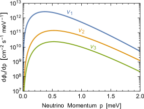
Figure 2: Isotropic $\nu$ or $\overline{\nu}$ differential flux today, $d\Phi_{\nu}/dp$, for neutrinos with mass as given in Eq. (5). The different curves correspond to our reference mass spectrum of Eq. (2).

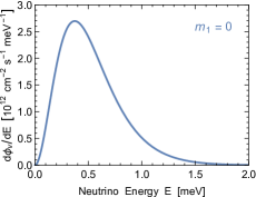
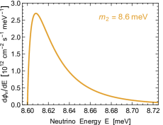
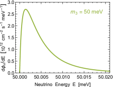
does not depend on $m_{\nu}$ and is $2.70\times 10^{12}~{}{\rm cm}^{-2}~{}{\rm s}^{-1}~{}{\rm meV}^{-1}$.

Figure 3: Neutrino differential flux $d\Phi_{\nu}/dE$ according to Eq. (6) for our reference mass spectrum of Eq. (2). The maximum flux

II.3 Spectrum at Earth

Which neutrino spectrum would be expected at Earth and should be shown on the GUNS plot? For neutrinos with mass, not the energy but the momentum is redshifted by cosmic expansion, so the phase-space occupation at redshift $z$ for free-streaming neutrinos is

$$f_{\nu}(p)=\frac{1}{e^{p/T_{z}}+1}\,,$$ (3)

where $T_{z}=T_{\nu}(1+z)$ and $T_{\nu}=1.945~{}{\rm K}$ is today’s temperature of hypothetical massless neutrinos. The present-day number density for one species of $\nu$ or $\overline{\nu}$, differential relative to momentum, is therefore

$$\frac{dn_{\nu}}{dp}=\frac{1}{2\pi^{2}}\,\frac{p^{2}}{e^{p/T_{\nu}}+1}\,.$$ (4)

Integration provides $n_{\nu}=56~{}{\rm cm}^{-3}$ as mentioned earlier.

Expressed as an isotropic flux, perhaps for a detection experiment, requires the velocity $p/E$ with $E=\sqrt{p^{2}+m_{i}^{2}}$, where $m_{i}$ is one of the mass eigenstates $i=1$, 2 or 3. So the isotropic differential flux today is

$$\frac{d\Phi_{\nu}}{dp}=\frac{p}{E}\frac{dn_{\nu}}{dp}=\frac{1}{2\pi^{2}}\,\frac{p^{3}}{\sqrt{p^{2}+m_{i}^{2}}}\,\frac{1}{e^{p/T_{\nu}}+1}\,.$$ (5)

In Fig. 2 we show this flux for our reference mass spectrum given in Eq. (2).

On the other hand, for plotting the GUNS, the spectrum in terms of energy is more useful. In this case we need to include a Jacobian $dp/dE=E/p$ that cancels the velocity factor so that

$$\frac{d\Phi_{\nu}}{dE}=\frac{p}{E}\frac{dn_{\nu}}{dE}=\frac{1}{2\pi^{2}}\,\frac{E^{2}-m_{i}^{2}}{e^{\sqrt{E^{2}-m_{i}^{2}}\big{/}T_{\nu}}+1}\,.$$ (6)

The maximum of this function does not depend on $m_{i}$ and is $2.70\times 10^{12}~{}{\rm cm}^{-2}~{}{\rm s}^{-1}~{}{\rm meV}^{-1}$. We show the energy spectrum for our reference neutrino masses in Fig. 3 and notice that for larger masses it is tightly concentrated at $E\gtrsim m_{i}$. Traditional GUNS plots Becker (2008); Spiering (2012) apply only to massless neutrinos.

These results ignore that the Earth is located in the gravitational potential of the Milky Way. Beginning with the momentum distribution of Eq. (4) we find for the average of the velocity $v=p/E$

$$\langle v\rangle=\frac{2700\,\zeta_{5}}{7\pi^{4}}\,\frac{T}{m}+{\cal O}\left(\frac{T}{m}\right)^{3}\approx 4.106\,\,\frac{T}{m}\,.$$ (7)

For $T=0.168~{}{\rm meV}$ and $m=50~{}{\rm meV}$ this is $\langle v\rangle=1.38\times 10^{-2}$, significantly larger than the galactic virial velocity of about $10^{-3}$. Therefore, gravitational clustering is a small effect Ringwald and Wong (2004); de Salas et al. (2017) and our momentum and energy distributions remain approximately valid if neutrino masses are as small as we have assumed.

One CNB mass eigenstate of $\nu_{i}$ plus $\bar{\nu}_{i}$ contributes at Earth a number and energy density of

$$n_{\nu\overline{\nu}} = 112~{}{\rm cm}^{-3}\ ,$$ (8)

$$\rho_{\nu\overline{\nu}} = \begin{cases}59.2~{}{\rm meV}~{}{\rm cm}^{-3}\kern 23.00006pt\quad\hbox{for $m_{\nu}\ll T_{\nu}$}\ ,\\ 112~{}{\rm meV}~{}{\rm cm}^{-3}~{}\frac{m_{\nu}}{{\rm meV}}\kern 3.00003pt\quad\hbox{for $m_{\nu}\gg T_{\nu}$}\ ,\end{cases}$$ (9)

ignoring small clustering effects in the galaxy. Here $T_{\nu}=1.95~{}{\rm K}=0.168~{}{\rm meV}$ as explained earlier.

The CNB consists essentially of an equal mixture of all flavors, so the probability for finding a random CNB $\nu$ or $\overline{\nu}$ in any of the mass eigenstates is equal to 1/3. Put another way, if the neutrino distribution is uniform among flavors and thus their flavor matrix is proportional to the unit matrix, this is true in any basis.

II.4 Detection perspectives

Directly measuring the CNB remains extremely challenging Ringwald (2009); Vogel (2015); Li (2017). Those ideas based on the electroweak potential on electrons caused by the cosmic neutrino sea Stodolsky (1975), an ${\cal O}(G_{\rm F})$ effect, depend on the net lepton number in neutrinos which today we know cannot be large as explained earlier and also would be washed out in the limit of nonrelativistic neutrinos. Early proposals based on the use of the neutrino wind Opher (1974); Lewis (1980) had been found to be not viable, as there is no net acceleration Cabibbo and Maiani (1982).

At ${\cal O}(G_{\rm F}^{2})$ one can also consider mechanical forces on macroscopic bodies by neutrino scattering and the annual modulation caused by the Earth’s motion in the neutrino wind Duda et al. (2001); Hagmann (1999), but the experimental realization of such ideas seems implausible with the available Cavendish-like balance technology. The results are not encouraging also for similar concepts based on interferometers Domcke and Spinrath (2017).

Another idea for the distant future is radiative atomic emission of a neutrino pair Yoshimura et al. (2015). The CNB affects this process by Pauli phase-space blocking.

Extremely high-energy neutrinos, produced as cosmic-ray secondaries or from ultra-heavy particle decay or cosmic strings, would be absorbed by the CNB, a resonant process if the CM energy matches the $Z^{0}$ mass Weiler (1982). For now there is no evidence for neutrinos in the required energy range beyond $10^{20}~{}{\rm eV}$ so that absorption dips cannot yet be looked for Ringwald (2009).

Perhaps the most realistic approach uses inverse $\beta$ decay Weinberg (1962); Cocco et al. (2007); Long et al. (2014); Arteaga et al. (2017); Lisanti et al. (2014); Akhmedov (2019), notably on tritium, $\nu_{e}+{\rm H}^{3}\to{\rm He}^{3}+e^{-}$, which is actually pursued by the PTOLEMY project Betts et al. (2013); Baracchini et al. (2018). However, our reference scenario with the mass spectrum given in Eq. (2) is particularly difficult because $\nu_{3}$ has the smallest $\nu_{e}$ admixture of all mass eigenstates. On the other hand, if the mass spectrum is inverted and/or quasi degenerate, the detection opportunities may be more realistic. Such an experiment may also be able to distinguish Dirac from Majorana neutrinos Long et al. (2014) and place constraints on nonstandard neutrino couplings Arteaga et al. (2017). Moreover, polarization of the target might achieve directionality Lisanti et al. (2014).

The properties of the CNB, the search for the neutrino mass scale, and the Dirac vs. Majorana question, remain at the frontier of particle cosmology and neutrino physics. Moreover, while neutrinos are but a small dark-matter component, detecting the CNB would be a first step in the future field of dark-matter astronomy.

III Neutrinos from Big-Bang Nucleosynthesis

During its first few minutes, the universe produces the observed light elements. Subsequent decays of neutrons ($n\to p+e+\overline{\nu}_{e}$) and tritons (${}^{3}{\rm H}\to{}^{3}{\rm He}+e+\overline{\nu}_{e}$) produce a very small $\overline{\nu}_{e}$ flux, which however dominates the GUNS in the gap between the CNB and thermal solar neutrinos roughly for $E_{\nu}=10$–100 meV. While a detection is currently out of the question, it would provide a direct observational window to primordial nucleosynthesis.

III.1 Primordial nucleosynthesis

Big-bang nucleosynthesis of the light elements is one of the pillars of cosmology Alpher et al. (1948); Alpher and Herman (1950); Steigman (2007); Iocco et al. (2009); Cyburt et al. (2016) and historically has led to a prediction of the CMB long before it was actually detected Gamow (1946); Alpher and Herman (1948, 1988). In the early universe, protons and neutrons are in $\beta$ equilibrium, so their relative abundance is $n/p=\exp(-\Delta m/T)$ with $\Delta m=1.293~{}{\rm MeV}$ their mass difference. Weak interactions freeze out about 1 s after the big bang when $T\approx 1~{}{\rm MeV}$, leaving $n/p\approx 1/6$. Nuclei form only 5 min later when $T$ falls below 60 keV and the large number of thermal photons no longer keeps nuclei dissociated. Neutrons decay, but their lifetime of 880 s leaves about $n/p\approx 1/7$ at that point. Subsequently most neutrons end up in ⁴He, leaving the famous primordial helium mass fraction of 25%.

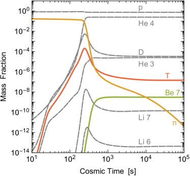
Figure 4: Evolution of light-element abundances in the early universe as indicated at the lines. Colored (solid) lines are neutrons (n) and the unstable isotopes tritium (T) and beryllium (⁷Be) that produce $\overline{\nu}_{e}$ and that do not survive until today. Plot was adapted from http://cococubed.asu.edu /code_pages/net_bigbang.shtml, where $\eta=6.23\times 10^{-10}$ and $H_{0}=70.5~{}{\rm km}~{}{\rm s}^{-1}~{}{\rm Mpc}^{-1}$ was used.

In detail, one has to solve a nuclear reaction network in the expanding universe and finds the evolution of light isotopes as shown in Fig. 4, where neutrons and the unstable isotopes are shown in color. Besides the nuclear-physics input, the result depends on the cosmic baryon fraction $\eta=n_{B}/n_{\gamma}$. With $\eta=6.23\times 10^{-10}$ that was chosen in Fig. 4 and the density $n_{\gamma}=411~{}{\rm cm}^{-3}$ of CMB photons, the baryon density is $n_{B}=2.56\times 10^{-7}~{}{\rm cm}^{-3}$. The 95% C.L. range for $n_{B}$ is 2.4–2.7 in these units Tanabashi et al. (2018). Of particular interest are the unstable but long-lived isotopes tritium (T) and ⁷Be for which Fig. 4 shows final mass fractions $1.4\times 10^{-7}$ and $3.1\times 10^{-9}$, corresponding to

$$n_{\rm T} = 1.2\times 10^{-14}~{}{\rm cm}^{-3},$$ (10a)

$$n_{\rm{}^{7}Be} = 1.1\times 10^{-16}~{}{\rm cm}^{-3}$$ (10b)

in terms of a present-day number density.

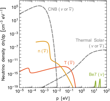
Figure 5: Density of low-energy neutrinos, taken to be massless ($p=E$). The CNB and thermal solar neutrinos include all flavors, but the lines are only for either $\nu$ or $\overline{\nu}$. Colored (solid) lines are BBN neutrinos: $\overline{\nu}_{e}$ from $n$ and tritium decay and $\nu_{e}$ from ⁷Be electron capture.

III.2 Neutrinos from decaying light isotopes

The isotopes shown in color in Fig. 4 are $\beta$ unstable and thus produce a small cosmic $\overline{\nu}_{e}$ or $\nu_{e}$ density which is much smaller than the CNB density given in Eq. (8), but shows up at larger energies because of less redshifting due to late decays Khatri and Sunyaev (2011); Ivanchik and Yurchenko (2018); Yurchenko and Ivanchik (2019). Ignoring for now the question of neutrino masses and flavor conversion, the resulting present-day number densities are shown in Fig. 5 in comparison with the CNB (Sec. II) and the low-energy tail of thermal solar neutrinos (Sec. V). These two sources produce $\nu\overline{\nu}$ pairs of all flavors, so their number density is equal for $\nu$ and $\overline{\nu}$. In Fig. 5 we show the all-flavor $\nu$ density of these sources, equal to that for $\overline{\nu}$, to compare with either the $\nu$ or $\overline{\nu}$ density of BBN neutrinos. The low-energy tail of traditional solar $\nu_{e}$ from nuclear reactions (Sec. IV) and of the $\overline{\nu}_{e}$ geoneutrino (Sec. VI) and reactor fluxes (Sec. VII) are all very much smaller than the solar thermal $\nu$ or $\overline{\nu}$ flux. One concludes that the BBN neutrinos ($\overline{\nu}_{e}$) from later neutron ($n$) and tritium decays produce the dominant density in the valley between the CNB and thermal solar neutrinos around neutrino energies of 10–200 meV. Of course, a detection of this flux is out of the question with present-day technology.

Beryllium recombination.—Considering the individual sources in more detail, we begin with ⁷Be which emerges with a much larger abundance than ⁷Li. Eventually it decays to ⁷Li by electron capture, producing $\nu_{e}$ of 861.8 keV (89.6%) or 384.2 keV (10.4%), analogous to the solar ⁷Be flux (Sec. IV). However, the electrons captured in the Sun are free, so their average energy increases by a thermal amount of a few keV (Table 1). In the dilute plasma of the early universe, electrons are captured from bound states, which happens only at around 900 years (cosmic redshift $z_{\rm rec}\approx 29,200$) when ⁷Be atoms form. The kinetics of ⁷Be recombination and decay was solved by Khatri and Sunyaev (2011) who found $z_{\rm rec}$ to be larger by about 5000 than implied by the Saha equation. The present-day energies of the lines are $13.1~{}{\rm eV}=384.2~{}{\rm keV}/(z_{\rm rec}+1)$ and $29.5~{}{\rm eV}=861.8~{}{\rm keV}/(z_{\rm rec}+1)$, each with a full width at half maximum of 7.8%, given by the redshift profile of ⁷Be recombination, i.e., 1.0 and 2.3 eV.

The ⁷Be lines in Fig. 5 were extracted from Fig. 5 of Khatri and Sunyaev (2011) with two modifications. The integrated number densities in the lines should be 10.4 : 89.6 according to the branching ratio of the ⁷Be decay, whereas in Khatri and Sunyaev (2011) the strength of the lower-energy line is reduced by an additional factor $(384.2/861.8)^{2}$ which we have undone. Moreover, we have multiplied both lines with a factor 5.6 to arrive at the number density $n_{\rm Be7}$ of Eq. (10). Notice that Khatri and Sunyaev (2011) cite a relative ⁷Be number density at the end of BBN of around $10^{-10}$, whereas their cited literature and also our Fig. 4 shows about 5–6 times more.

Tritium decay.—BBN produces a tritium (T or ³H) abundance given in Eq. (10) which later decays with a lifetime of 17.8 years by ${}^{3}{\rm H}\to{}^{3}{\rm He}+e+\overline{\nu}_{e}$, producing the same number density of $\overline{\nu}_{e}$ with a spectral shape given by Eq. (17) with $E_{\rm max}=18.6$ keV. During radiation domination, a cosmic age of 17.8 years corresponds to a redshift of $2\times 10^{5}$, so an energy of 18.6 keV is today 90 meV, explaining the $\overline{\nu}_{e}$ range shown in Fig. 5.

This spectrum was taken from Fig. 2 of Ivanchik and Yurchenko (2018). Pre-asymptotic tritium (i.e. the population existing at the onset of BBN, identified by the spike in Fig. 4) was also included, producing the low-energy step-like feature. The isotropic flux shown by Ivanchik and Yurchenko (2018) was multiplied with a factor $2/c$ to obtain our number density. Our integrated $\overline{\nu}_{e}$ density then corresponds well to the tritium density in Eq. (10).

Neutron decay.—After weak-interaction freeze-out near 1 sec, neutrons decay with a lifetime of 880 s, producing $\overline{\nu}_{e}$ with a spectrum given by Eq. (17) with $E_{\rm max}=782~{}{\rm keV}$. The short lifetime implies that there is no asymptotic value around the end of BBN. Notice also that the late $n$ evolution shown in Fig. 5 is not explained by decay alone that would imply a much faster decline, i.e., residual nuclear reactions provide a late source of neutrons. The $\overline{\nu}_{e}$ number density shown in Fig. 5 was obtained from Ivanchik and Yurchenko (2018) with the same prescription that we used for tritium.

III.3 Neutrinos with mass

The cross-over region between CNB, BBN, and solar neutrinos shown in Fig. 5 is at energies where sub-eV neutrino masses become important. For the purpose of illustration we use the minimal masses in normal ordering of Eq. (2) with 0, 8.6, and 50 meV. Neutrinos reaching Earth will have decohered into mass eigenstates, so one needs to determine the three corresponding spectra.

The CNB consists essentially of an equal mixture of all flavors, so the probability for finding a random CNB neutrino or antineutrino in any of the mass eigenstates is

$$P_{i}^{\rm CNB}=\frac{1}{3}\quad\hbox{for}\quad i=1,2,3.$$ (11)

The flavor density matrix is essentially proportional to the unit matrix from the beginning and thus is the same in any basis. Flavor conversion has no effect.

On the other hand, the BBN neutrinos are produced in the $e$ flavor, so their flavor content will change with time. Flavor evolution in the early universe can involve many complications in that the matter effect at $T\gtrsim 1$ MeV is dominated by a thermal term Nötzold and Raffelt (1988). Moreover, neutrinos themselves are an important background medium, leading to collective flavor evolution Kostelecky et al. (1993); Duan et al. (2010).

However, the BBN neutrinos are largely produced after BBN is complete at $T\lesssim 60$ MeV. Scaling the present-day baryon density of $2.5\times 10^{-7}~{}{\rm cm}^{-3}$ to the post-BBN epoch provides a matter density of the order of $10^{-5}~{}{\rm g}~{}{\rm cm}^{-3}$, very much smaller than the density of Sun or Earth, so the matter or neutrino backgrounds are no longer important. For the purpose of flavor evolution of MeV-range neutrinos we are in vacuum and the mass-content of the original states does not evolve. So we may use the best-fit probabilities $P_{ei}$ of finding a $\nu_{e}$ or $\overline{\nu}_{e}$ in any of the mass eigenstates given in the top row of Eq. (64),

$$P_{1}^{\rm BBN}=0.681,\quad P_{2}^{\rm BBN}=0.297,\quad P_{3}^{\rm BBN}=0.022.$$ (12)

Notice that here we have forced the numbers to add up to unity to correct for rounding errors.

Thermal solar neutrinos emerge in all flavors, but not with equal probabilities Vitagliano et al. (2017). For very low energies, the mass-eigenstate probabilities are (see text below Eq. 25)

$$P_{1}^{\rm Sun}=0.432,\quad P_{2}^{\rm Sun}=0.323,\quad P_{3}^{\rm Sun}=0.245.$$ (13)

For higher energies, these probabilities are plotted in the bottom panel of Fig. 12.

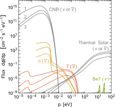
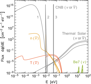
Figure 6: Flux densities of mass-eigenstate neutrinos for $m_{i}=0$, 8.6 and 50 meV as indicated at the curves, using the probabilities of Eqs. (11–13) and the spectra of Fig. 5. Top: $d\Phi/dp$ which includes a velocity factor $v_{i}=p/E_{i}$ for each mass state. Bottom: $d\Phi/dE$ showing sharp lines at $E=m_{2,3}$.

The CNB and BBN neutrinos are produced with high energies and later their momenta are redshifted by cosmic expansion. Therefore, their comoving differential number spectrum $dn/dp$ as a function of $p$ remains unchanged. If we interpret the horizontal axis of Fig. 5 as $p$ instead of $E$ and the vertical axis as $dn/dp$ instead of $dn/dE$, the CNB and BBN curves actually do not change, except that we get three curves, one for each mass eigenstate, with the relative amplitudes of Eqs. (11) and (12).

For thermal solar neutrinos, the same argument applies to bremsstrahlung, which dominates at low energies, because the spectrum is essentially determined by phase space alone (Sec. V.3). At higher energies, where our assumed small masses are not important, the mass would also enter in the matrix element and one would need an appropriate evaluation of plasmon decay.

For experimental searches, the flux may be a more appropriate quantity. Multiplying the number density spectra of Fig. 5 for each $p$ with the velocity $v_{i}=p/\sqrt{p^{2}+m_{i}^{2}}$ provides the mass-eigenstate flux spectra $d\Phi/dp$ shown in Fig. 6 (top), in analogy to Fig. 2.

For experiments considering the absorption of neutrinos, e.g. inverse $\beta$ decay on tritium, the energy $E$ is a more appropriate variable instead of the momentum $p$, so we show $d\Phi/dE$ as a function of $E$ in Fig. 6 (bottom). Notice that the velocity factor $v_{i}$ is undone by a Jacobian $E/p$, so for example the maxima of the mass-eigenstate curves are the same for every $m_{i}$ as discussed in Sec. II.3 and illustrated in Fig. 3. Relative to the massless case of Fig. 5, the vertical axis is simply scaled with a factor $c$, whereas the curves are compressed in the horizontal direction by $p\to E=\sqrt{p^{2}+m_{i}^{2}}$. Effectively one obtains narrow lines at the non-vanishing neutrino masses that are vastly dominated by the CNB. The integrated fluxes of the three mass eigenstates in either $\nu$ or $\overline{\nu}$ are

$$\Phi_{1} = 1.68\times 10^{12}~{}{\rm cm}^{-2}~{}{\rm s}^{-1},$$ (14a)

$$\Phi_{2} = 1.35\times 10^{11}~{}{\rm cm}^{-2}~{}{\rm s}^{-1},$$ (14b)

$$\Phi_{3} = 2.32\times 10^{10}~{}{\rm cm}^{-2}~{}{\rm s}^{-1},$$ (14c)

where we have used Eqs. (7) and (8) of Sec. II.

Note that we have assumed $m_{1}=0$ in this Section; a degenerate mass spectrum (i.e., $m_{1}\gg T_{\nu}=0.168$ meV) would make the flux densities of all mass eigenstates similar to each other, they will all have a spike-like behavior, and they will be shifted to larger energies. In this case there is no neutrino radiation in the universe today, only neutrino hot dark matter.

IV Solar Neutrinos from Nuclear Reactions

The Sun emits 2.3% of its nuclear energy production in the form of MeV-range electron neutrinos. They arise from the effective fusion reaction $4p+2e^{-}\to{}^{4}{\rm He}+2\nu_{e}+26.73~{}{\rm MeV}$ that proceeds through several reaction chains and cycles. The history of solar neutrino measurements is tightly connected with the discovery of flavor conversion and the matter effect on neutrino dispersion. There is also a close connection to precision modeling of the Sun, leading to a new problem in the form of discrepant sound-speed profiles relative to helioseismology. This issue may well be related to the photon opacities and thus to the detailed chemical abundances in the solar core, a prime target of future neutrino precision experiments. Meanwhile, solar neutrinos are becoming a background to weakly interacting massive particle (WIMP) dark-matter searches. In fact, dark-matter detectors in future may double as solar neutrino observatories.

IV.1 The Sun as a neutrino source

The Sun produces nuclear energy by hydrogen fusion to helium that proceeds through the pp chains (exceeding 99% for solar conditions) and the rest through the CNO cycle Clayton (1983); Kippenhahn et al. (2012); Bahcall and Ulrich (1988); Bahcall (1989); Haxton et al. (2013); Serenelli (2016). For every produced ${}^{4}{\rm He}$ nucleus, two protons need to convert to neutrons by what amounts to $p+e^{-}\to n+\nu_{e}$, i.e., two electrons disappear in the Sun and emerge as $\nu_{e}$. The individual $\nu_{e}$-producing reactions are listed in Table 1 (for more details see below) and the expected flux spectra at Earth are shown in Fig. 7.

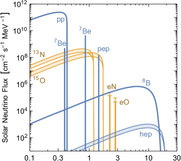
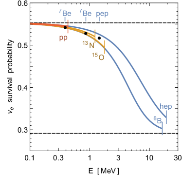
Figure 7: Solar neutrinos from different source reactions. In blue (dark gray) pp-chain neutrinos (pp, ⁷Be, pep, ⁸B, hep), in orange (light gray) CNO neutrinos (¹³N, ¹⁵O and the electron-capture lines eN and eO). Top panel: Differential fluxes, where line sources are in units of $\rm{cm}^{-2}~{}\rm{s}^{-1}$. pp-chain fluxes (except for hep) according to the measurements shown in Table 1 where the uncertainties are too small to show. For the CNO and hep fluxes the range is bracketed by the lowest AGSS09 and highest GS98 predictions. ¹⁷F is a very small correction to the ¹⁵O flux and thus not shown. Bottom panel: Adiabatic $\nu_{e}$ survival probability due to flavor conversion (see Sec. IV.5) which depends on the radial distributions of the different production processes. For the eN and eO lines, these distributions have not been published. The black dots show the survival probabilities of the three pp-chain lines from ⁷Be and pep. The horizontal dashed lines show the survival probability for vanishing and infinite neutrino energy.

Table 1: Neutrino fluxes at Earth from different nuclear reactions in the Sun. Theoretical predictions from Vinyoles et al. (2017) for models with GS98 Grevesse and Sauval (1998) and AGSS09 Asplund et al. (2009) abundances. The predicted electron capture (EC) fluxes from the CNO cycle were obtained by scaling the $\beta^{+}$-decay fluxes Stonehill et al. (2004). The neutrino endpoint energy $E_{\rm max}$ and average $E_{\rm av}$ includes thermal energy of a few keV Bahcall (1997) except for the CNO-EC lines, where the given $E_{\rm av}$ is $E_{\rm max}+2m_{e}$ of the corresponding $\beta^{+}$ process. Observed fluxes with $1\sigma$ errors from the global analysis of Bergström et al. (2016).

Channel	Flux	Reaction	$E_{\rm av}$	$E_{\rm max}$	Flux at Earth
			MeV	MeV	GS98		AGSS09		Observed	Units
pp Chains ($\beta^{+}$)	$\Phi_{\rm pp}$	$p+p\rightarrow d+e^{+}+\nu_{e}$	0.267	0.423	5.98	$\pm 0.6\%$	6.03	$\pm 0.5\%$	$5.971^{+0.62\%}_{-0.55\%}$	$10^{10}~{}{\rm cm}^{-2}~{}{\rm s}^{-1}$
	$\Phi_{\rm B}$	$\ce{{}^{8}B}\rightarrow\ce{{}^{8}Be^{*}}+e^{+}+\nu_{e}$	$6.735\pm 0.036$	$\sim 15$	5.46	$\pm 12\%$	4.50	$\pm 12\%$	$5.16^{+2.5\%}_{-1.7\%}$	$10^{6}~{}{\rm cm}^{-2}~{}{\rm s}^{-1}$
	$\Phi_{\rm hep}$	$\ce{{}^{3}He}+p\rightarrow\ce{{}^{4}He}+e^{+}+\nu_{e}$	9.628	18.778	0.80	$\pm 30\%$	0.83	$\pm 30\%$	$1.9^{+63\%}_{-47\%}$	$10^{4}~{}{\rm cm}^{-2}~{}{\rm s}^{-1}$
pp Chains (EC)	$\Phi_{\rm Be}$	$e^{-}+\ce{{}^{7}Be}\rightarrow\ce{{}^{7}Li}+\nu_{e}$	0.863 (89.7%)		4.93	$\pm 6\%$	4.50	$\pm 6\%$	$4.80^{+5.9\%}_{-4.6\%}$	$10^{9}~{}{\rm cm}^{-2}~{}{\rm s}^{-1}$
		$e^{-}+\ce{{}^{7}Be}\rightarrow\ce{{}^{7}Li^{*}}+\nu_{e}$	0.386 (10.3%)
	$\Phi_{\rm pep}$	$p+e^{-}+p\rightarrow d+\nu_{e}$	1.445		1.44	$\pm 1\%$	1.46	$\pm 0.9\%$	$1.448^{+0.90\%}_{-0.90\%}$	$10^{8}~{}{\rm cm}^{-2}~{}{\rm s}^{-1}$
CNO Cycle ($\beta^{+}$)	$\Phi_{\rm N}$	$\ce{{}^{1}3N}\rightarrow\ce{{}^{1}3C}+e^{+}+\nu_{e}$	0.706	1.198	2.78	$\pm 15\%$	2.04	$\pm 14\%$	${}<13.7$	$10^{8}~{}{\rm cm}^{-2}~{}{\rm s}^{-1}$
	$\Phi_{\rm O}$	$\ce{{}^{1}5O}\rightarrow\ce{{}^{1}5N}+e^{+}+\nu_{e}$	0.996	1.732	2.05	$\pm 17\%$	1.44	$\pm 16\%$	${}<2.8$	$10^{8}~{}{\rm cm}^{-2}~{}{\rm s}^{-1}$
	$\Phi_{\rm F}$	$\ce{{}^{1}7F}\rightarrow\ce{{}^{1}7O}+e^{+}+\nu_{e}$	0.998	1.736	5.29	$\pm 20\%$	3.26	$\pm 18\%$	${}<8.5$	$10^{6}~{}{\rm cm}^{-2}~{}{\rm s}^{-1}$
CNO Cycle (EC)	$\Phi_{\rm eN}$	$\ce{{}^{1}3N}+e^{-}\rightarrow\ce{{}^{1}3C}+\nu_{e}$	2.220		2.20	$\pm 15\%$	1.61	$\pm 14\%$	—	$10^{5}~{}{\rm cm}^{-2}~{}{\rm s}^{-1}$
	$\Phi_{\rm eO}$	$\ce{{}^{1}5O}+e^{-}\rightarrow\ce{{}^{1}5N}+\nu_{e}$	2.754		0.81	$\pm 17\%$	0.57	$\pm 16\%$	—	$10^{5}~{}{\rm cm}^{-2}~{}{\rm s}^{-1}$
	$\Phi_{\rm eF}$	$\ce{{}^{1}7F}+e^{-}\rightarrow\ce{{}^{1}7O}+\nu_{e}$	2.758		3.11	$\pm 20\%$	1.91	$\pm 18\%$	—	$10^{3}~{}{\rm cm}^{-2}~{}{\rm s}^{-1}$

All pp chains begin with $p+p\to d+e^{+}+\nu_{e}$, the pp reaction, which on average releases 0.267 MeV as $\nu_{e}$. Including other processes (GS98 predictions of Table 1) implies $\langle E_{\nu_{e}}\rangle=0.312~{}{\rm MeV}$. The solar luminosity without neutrinos is $L_{\odot}=3.828\times 10^{33}~{}{\rm erg}~{}{\rm s}^{-1}=2.39\times 10^{39}~{}{\rm MeV}~{}{\rm s}^{-1}$, implying a solar $\nu_{e}$ production of

$$L_{\nu_{e}}=2\times\frac{L_{\odot}}{26.73~{}\rm{MeV}-2\,\langle E_{\nu_{e}}\rangle}=1.83\times 10^{38}~{}{\rm s}^{-1},$$ (15)

where 26.73 MeV is the energy released per He fusion and $2$ the number of neutrinos per fusion. The average distance of $1.496\times 10^{13}~{}{\rm cm}$ thus implies a flux, number density, and energy density at Earth of

$$\Phi_{\nu} = 6.51\times 10^{10}~{}{\rm cm}^{-2}~{}{\rm s}^{-1},$$ (16a)

$$n_{\nu} = 2.17~{}{\rm cm}^{-3},$$ (16b)

$$\rho_{\nu} = 0.685~{}{\rm MeV}~{}{\rm cm}^{-3}.$$ (16c)

These numbers change by $\pm 3.4\%$ in the course of the year due to the ellipticity of the Earth’s orbit, a variation confirmed by the Super-Kamiokande detector Fukuda et al. (2001).

While this overall picture is robust, the flux spectra of those reactions with larger $E_{\nu_{e}}$ are particulary important for detection and flavor-oscillation physics, but are side issues for overall solar physics. Therefore, details of the production processes and of solar modeling are crucial for predicting the solar neutrino spectrum.

IV.2 Production processes and spectra

The proton-neutron conversion required for hydrogen burning proceeds either as $\beta^{+}$ decay of the effective form $p\to n+e^{+}+\nu_{e}$, producing a continuous spectrum, or as electron capture (EC) $e^{-}+p\to n+\nu_{e}$, producing a line spectrum. The nuclear MeV energies imply a much larger final-state $\beta^{+}$ phase space than the initial-state phase space occupied by electrons with keV thermal energies, so the continuum fluxes tend to dominate Bahcall (1990).

Line energies are larger $+2m_{e}$ relative to the continuum end point) and lines produce a distinct detection signature Bellini et al. (2014); Agostini et al. (2019). The ${}^{7}{\rm Be}$ line is particularly important because the nuclear energy is too small for $\beta^{+}$ decay. (Actually in 10% of all cases it proceeds through an excited state of ${}^{7}{\rm Li}$, so there are two lines, together forming the ${}^{7}{\rm Be}$ flux.)

We neglect ${}^{3}{\rm He}+e^{-}+p\to{}^{4}{\rm He}+\nu_{e}$, the heep flux Bahcall (1990). On the other hand, we include the often neglected lines from EC in CNO reactions, also called ecCNO processes Stonehill et al. (2004); Villante (2015). Our flux predictions come from scaling the continuum fluxes Vinyoles et al. (2017) with the ratios provided by Stonehill et al. (2004), although these are based on a different solar model. This inconsistency is small compared with the overall uncertainty of the CNO fluxes.

The endpoint $E_{\rm max}$ of a continuum spectrum is given, in vacuum, by the nuclear transition energy. However, for the reactions taking place in the Sun one needs to include thermal kinetic energy of a few keV. The endpoint and average energies listed in Table 1 include this effect according to Bahcall Bahcall (1997). For the same reason the EC lines are slightly shifted and have a thermal width of a few keV Bahcall (1993), which is irrelevant in practice for present-day experiments. The energies of the ecCNO lines were obtained from the listed continuum endpoints by adding $2m_{e}$, which agrees with Stonehill et al. (2004) except for ${}^{17}{\rm F}$, where they show 2.761 instead of 2.758 MeV.

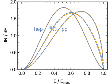
Figure 8: Spectra of pp, ¹⁵O and hep neutrinos. The other CNO spectra are similar to ¹⁵O. Solid: Tabulated spectra according to Bahcall (1997). Dashed: Allowed nuclear decay spectra according to Eq. (17).

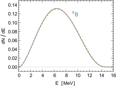
Figure 9: Spectrum of ⁸B neutrinos. Solid: According to Bahcall et al. (1996). Dashed: According to Winter et al. (2006).

Except for ⁸B, the continuum spectra follow from an allowed nuclear $\beta$ decay, being dominated by the phase space of the final-state $e^{+}$ and $\nu_{e}$. In vacuum and ignoring $e^{+}$ final-state interactions it is

$$\frac{dN}{dE}\propto E^{2}(Q-E)\sqrt{(Q-E)^{2}-m_{e}^{2}}\,,$$ (17)

where $Q=E_{\rm max}+m_{e}$. In Fig. 8 (dashed lines) we show these spectra in normalized form for the pp and hep fluxes as well as ${}^{15}{\rm O}$, representative of the CNO fluxes. We also show the spectra (solid lines), where final-state corrections and thermal initial-state distributions are included according to Bahcall (1997). Notice that the spectra provided on the late John Bahcall’s homepage are not always exactly identical with those in Bahcall (1997).

The ⁸B flux is the dominant contribution in many solar neutrino experiments because it reaches to large energies and the detection cross section typically scales with $E^{2}$, yet it is the one with the least simple spectrum. The decay ${}^{8}{\rm B}\to{}^{8}{\rm Be}+e^{+}+\nu_{e}$ has no sharp cutoff because the final-state ${}^{8}{\rm Be}$ is unstable against $2\alpha$ decay. The $\nu_{e}$ spectrum can be inferred from the measured $\alpha$ and $\beta^{+}$ spectra. The $\nu_{e}$ spectrum provided by Bahcall et al. (1996) is shown in Fig. 9 as a solid line. As a dashed line we show the determination of Winter et al. (2006), based on a new measurement of the $\alpha$ spectrum.

For comparison with keV thermal neutrinos (Sec. V) it is useful to consider an explicit expression for the solar flux at low energies where the pp flux strongly dominates. Using the observed total pp flux from Table 1, we find that an excellent approximation for the flux at Earth is

$$\frac{d\Phi_{\rm pp}}{dE}=\frac{832.7\times 10^{10}}{{\rm cm}^{2}~{}{\rm s}~{}{\rm MeV}}\,\left(\frac{E}{{\rm MeV}}\right)^{2}\left(1-2.5\,\frac{E}{{\rm MeV}}\right).$$ (18)

To achieve sub-percent precision, the purely quadratic term can be used for $E$ up to a few keV. With the next correction, the expression can be used up to 100 keV.

IV.3 Standard solar models

The neutrino flux predictions, such as those shown in Table 1, depend on a detailed solar model that provides the variation of temperature, density, and chemical composition with radius. While the neutrino flux from the dominant pp reaction is largely determined by the overall luminosity, the small but experimentally dominant higher-energy fluxes depend on the branching between different terminations of the pp chains and the relative importance of the CNO cycle, all of which depends sensitively on chemical composition and temperature. For example, the ${}^{8}{\rm B}$ flux scales approximately as $T_{\rm c}^{24}$ with solar core temperature Bahcall and Ulmer (1996) — the neutrino fluxes are sensitive solar thermometers.

The flux predictions are usually based on a Standard Solar Model (SSM) Serenelli (2016), although the acronym might be more appropriately interpreted as Simplified Solar Model. One assumes spherical symmetry and hydrostatic equilibrium, neglecting dynamical effects, rotation, and magnetic fields. The zero-age model is taken to be chemically homogeneous without further mass loss or gain. Energy is transported by radiation (photons) and convection. The latter is relevant only in the outer region (2% by mass or 30% by radius) and is treated phenomenologically with the adjustable parameter $\alpha_{\rm MLT}$ to express the mixing length in terms of the pressure scale height.

Further adjustable parameters are the initial mass fractions of hydrogen, $X_{\rm ini}$, helium, $Y_{\rm ini}$, and “metals” (denoting anything heavier than helium), $Z_{\rm ini}$, with the constraint $X_{\rm ini}+Y_{\rm ini}+Z_{\rm ini}=1$. These parameters must be adjusted such that the evolution to the present age of $\tau_{\odot}=4.57\times 10^{9}~{}{\rm years}$ reproduces the measured luminosity $L_{\odot}=3.8418\times 10^{33}~{}{\rm erg}~{}{\rm s}^{-1}$, the radius $R_{\odot}=6.9598\times 10^{10}~{}{\rm cm}$, and the spectroscopically observed metal abundance at the surface, $Z_{\rm S}$, relative to that of hydrogen, $X_{\rm S}$. These surface abundances differ from the initial ones because of gravitational settling of heavier elements relative to lighter ones. As an example we show in Fig. 10 the radial variation of several solar parameters for a SMM of the Barcelona group Vinyoles et al. (2017).

The relative surface abundances of different elements are determined by spectroscopic measurements which agree well, for non-volatile elements, with those found in meteorites. The older standard abundances (GS98) of Grevesse and Sauval (1998) were superseded in 2009 by the AGSS09 composition of Asplund, Grevesse, Sauval and Scott and updated in 2015 Asplund et al. (2009); Scott et al. (2015b, a); Grevesse et al. (2015). The AGSS09 composition shows significantly smaller abundances of volatile elements. According to Vinyoles et al. (2017), the surface abundances are $Z_{\rm S}=0.0170\pm 0.0012$ (GS98) and $0.0134\pm 0.0008$ (AGSS09), the difference being almost entirely due to CNO elements.

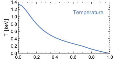
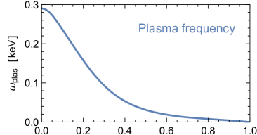
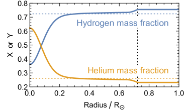
Figure 10: Standard Solar Model of the Barcelona group Vinyoles et al. (2017) with AGSS09 composition. Bottom panel: The vertical dotted line shows $R_{\rm CZ}$, the depth of the convection zone, whereas the horizontal lines show the initial H and He mass fractions.

The CNO abundances not only affect CNO neutrino fluxes directly, but determine the solar model through the photon opacities that regulate radiative energy transfer. Theoretical opacity calculations include OPAL Iglesias and Rogers (1996), the Opacity Project (OP) Badnell et al. (2005), OPAS Blancard et al. (2012); Mondet et al. (2015), STAR Krief et al. (2016), and OPLIB Colgan et al. (2016), which for solar conditions agree within 5%, but strongly depend on input abundances.

A given SSM can be tested with helioseismology that determines the sound-speed profile, the depth of the convective zone, $R_{\rm CZ}$, and the surface helium abundance, $Y_{\rm S}$. The new spectroscopic surface abundances immediately caused a problem in that these parameters deviate significantly from the solar values, whereas the old GS98 abundances provide much better agreement Vinyoles et al. (2017); Grevesse and Sauval (1998); Asplund et al. (2009). (See Table 2 for a comparison using recent Barcelona models.)

So while SSMs with the old GS98 abundances provide good agreement with helioseismology, they disagree with the modern surface abundances, whereas for the AGSS09 class of models it is the other way around. There is no satisfactory solution to this conundrum, which is termed the “solar abundance problem,” although it is not clear if something is wrong with the abundances, the opacity calculations, other input physics, or any of the assumptions entering the SSM framework.

Table 2: Main characteristics of two Barcelona SSMs of Vinyoles et al. (2017) with GS98 and AGSS09 abundances. $R_{\rm CZ}$ is the depth of the convection zone and $\langle\delta c/c\rangle$ the average deviation of the sound-speed profile relative to helioseismic measurements.

Quantity	B16-GS98	B16-AGSS09	Solar
$Y_{\rm S}$	$0.2426\pm 0.0059$	$0.2317\pm 0.0059$	$0.2485\pm 0.0035$
$R_{\rm CZ}/R_{\odot}$	$0.7116\pm 0.0048$	$0.7223\pm 0.0053$	$0.713\pm 0.001$
$\langle\delta c/c\rangle$	$0.0005^{+0.0006}_{-0.0002}$	$0.0021\pm 0.001$	—
$\alpha_{\rm MLT}$	$2.18\pm 0.05$	$2.11\pm 0.05$	—
$Y_{\rm ini}$	$0.2718\pm 0.0056$	$0.2613\pm 0.0055$	—
$Z_{\rm ini}$	$0.0187\pm 0.0013$	$0.0149\pm 0.0009$	—
$Z_{\rm S}$	$0.0170\pm 0.0012$	$0.0134\pm 0.0008$	—

The pp-chains neutrino fluxes predicted by these two classes of models bracket the measurements (Table 1), which however do not clearly distinguish between them. A future measurement of the CNO fluxes might determine the solar-core CNO abundances and thus help to solve the “abundance problem.” While it is not assured that the two classes of models actually bracket the true case, one may speculate that the CNO fluxes might lie between the lowest AGSS09 and the largest GS98 predictions. Therefore, this range is taken to define the flux prediction shown in Fig. 7.

IV.4 Antineutrinos

The Borexino scintillator detector has set the latest limit on the flux of solar $\overline{\nu}_{e}$ at Earth of $760~{}{\rm cm}^{-2}~{}{\rm s}^{-1}$, assuming a spectral shape of the undistorted ⁸B $\nu_{e}$ flux and using a threshold of 1.8 MeV Bellini et al. (2011). This corresponds to a 90% C.L. limit on a putative $\nu_{e}\to\overline{\nu}_{e}$ transition probability of $1.3\times 10^{-4}$ for $E_{\nu}>1.8~{}{\rm MeV}$.

In analogy to the geoneutrinos of Sec. VI, the Sun contains a small fraction of the long-lived isotopes ⁴⁰K, ²³²Th, and ²³⁸U that produce a $\overline{\nu}_{e}$ flux Malaney et al. (1990). However, it is immediately obvious that at the Earth’s surface, this solar flux must be much smaller than that of geoneutrinos. If the mass fraction of these isotopes were the same in the Sun and Earth and if their distribution in the Earth were spherically symmetric, the fluxes would have the proportions of $M_{\odot}/D_{\odot}^{2}$ vs. $M_{\oplus}/R_{\oplus}^{2}$, with the solar mass $M_{\odot}$, its distance $D_{\odot}$, the Earth mass $M_{\oplus}$, and its radius $R_{\oplus}$. So the solar flux would be smaller in the same proportion as the solar gravitational field is smaller at Earth, i.e., about $6\times 10^{-4}$ times smaller.

The largest $\overline{\nu}_{e}$ flux comes from ⁴⁰K decay. The solar potassium mass fraction is around $3.5\times 10^{-6}$ Asplund et al. (2009), the relative abundance of the isotope ⁴⁰K is 0.012%, so the ⁴⁰K solar mass fraction is $4\times 10^{-10}$, corresponding to $8\times 10^{23}~{}{\rm g}$ of ⁴⁰K in the Sun or $1.3\times 10^{46}$ atoms. With a lifetime of $1.84\times 10^{9}$ years, the $\overline{\nu}_{e}$ luminosity is $2\times 10^{29}~{}{\rm s}^{-1}$ or a flux at Earth of around $100~{}{\rm cm}^{-2}~{}{\rm s}^{-1}$. With a geo-$\overline{\nu}_{e}$ luminosity of around $2\times 10^{25}~{}{\rm s}^{-1}$ from potassium decay (Sec. VI), the average geoneutrino flux is $5\times 10^{6}~{}{\rm cm}^{-2}~{}{\rm s}^{-1}$ at the Earth’s surface, although with large local variations.

An additional flux of higher-energy solar $\overline{\nu}_{e}$ comes from photo fission of heavy elements such as uranium by the 5.5 MeV photon from the solar fusion reaction $p+d\to{}^{3}{\rm He}+\gamma$ Malaney et al. (1990). One expects a $\overline{\nu}_{e}$ spectrum similar to a power reactor, where fission is caused by neutrons. However, this tiny flux of around $10^{-3}~{}{\rm cm}^{-2}~{}{\rm s}^{-1}$ is vastly overshadowed by reactor $\overline{\nu}_{e}$.

IV.5 Flavor conversion

While solar neutrinos are produced as $\nu_{e}$, the flux at Earth shown in Fig. 7 (top) has a different composition because of flavor conversion on the way out of the Sun. The long distance between Sun and Earth relative to the vacuum oscillation length implies that the propagation eigenstates effectively decohere, so we can picture the neutrinos arriving at Earth to be mass eigenstates. These can be re-projected on interaction eigenstates, notably on $\nu_{e}$, if the detector is flavor sensitive.

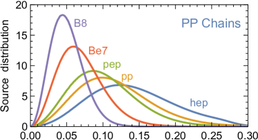
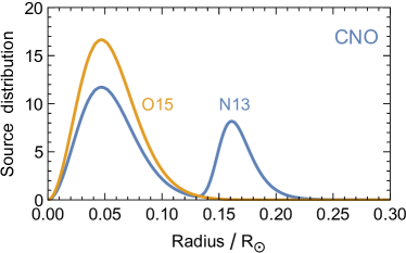
Figure 11: Normalised distribution of neutrino production for the indicated source reactions according to the SSM of the Barcelona group Vinyoles et al. (2017) with AGSS09 composition. In the CNO cycle, the ¹⁷F distribution is very similar to that of ¹⁵O.

Flavor conversion of solar neutrinos is almost perfectly adiabatic and, because of the hierarchy of neutrino mass differences, well approximated by an effective two-flavor treatment. The probability of a produced $\nu_{e}$ to emerge at Earth in any of the three mass eigenstates is given by Eq. (77) and the probability to be measured as a $\nu_{e}$, the survival probability, by Eq. (78). For the limiting case of very small $E_{\nu}$, the matter effect is irrelevant and

$$P_{ee}^{\rm vac}=\frac{1+\cos^{2}2\theta_{12}}{2}\,\cos^{4}\theta_{13}+\sin^{4}\theta_{13}=0.533,$$ (19)

corresponding to the best-fit mixing parameters in normal ordering. In the other extreme of large energy or large matter density, one finds

$$P_{ee}^{\infty}=\frac{1-\cos 2\theta_{12}}{2}\,\cos^{4}\theta_{13}+\sin^{4}\theta_{13}=0.292.$$ (20)

These extreme cases are shown as horizontal dashed lines in the lower panel of Fig. 7. Otherwise, $P_{ee}$ depends on the weak potential at the point of production, so $P_{ee}$ for a given $E_{\nu}$ depends on the radial source distributions in the Sun. These are shown in Fig. 11 according to an AGSS09 model of the Barcelona group, using the best-fit mixing parameters in normal ordering. Notice that such distributions for the EC-CNO reactions have not been provided, but would be different from the continuum processes. The survival probabilities for the different source processes are shown in the lower panel of Fig. 7. As we see from the radial distributions of ${}^{8}{\rm B}$ and hep, the corresponding curves in Fig. 7 essentially bracket the range of survival probabilities for all processes.

While neutrinos arriving at Earth have decohered into mass eigenstates, propagation through the Earth causes flavor oscillations, producing coherent superpositions at the far end. So if the solar flux is observed through the Earth (“at night”), this small effect needs to be included. This day-night asymmetry for the ⁸B flux was measured by the Super-Kamiokande detector to be Renshaw et al. (2014); Abe et al. (2016)

$$A_{\rm DN} = \frac{\Phi_{\rm day}-\Phi_{\rm night}}{(\Phi_{\rm day}+\Phi_{\rm night})/2}$$ (21)

$$= \bigl{(}-3.3\pm 1.0_{\rm stat}\pm 0.5_{\rm syst}\bigr{)}\%\,,$$

corresponding to a $2.9\,\sigma$ significance. As measured in $\nu_{e}$, the Sun shines brighter at night!

The energy-dependent $\nu_{e}$ survival probability for ⁸B neutrinos shown in the lower panel of Fig. 7 implies a spectral deformation of the measured flux relative to the ⁸B source spectrum. The latest Super-Kamiokande analysis Abe et al. (2016) is consistent with this effect, but also consistent with no distortion at all.

IV.6 Observations and detection perspectives

Solar neutrino observations have a 50-year history, beginning in 1968 with the Homestake experiment Davis et al. (1968); Cleveland et al. (1998), a pioneering achievement that earned Raymond Davis the Physics Nobel Prize (2002). Homestake was based on the radiochemical technique of ${}^{37}{\rm Cl}(\nu_{e},e^{-}){}^{37}{\rm Ar}$ and subsequent argon detection, registering approximately 800 solar $\nu_{e}$ in its roughly 25 years of data taking that ended in 1994. Since those early days, many experiments have measured solar neutrinos Wurm (2017), and in particular Super-Kamiokande Abe et al. (2016), based on elastic scattering on electrons measured by Cherenkov radiation in water, has registered around 80,000 events since 1996 and has thus become sensitive to percent-level effects. The chlorine experiment was mainly sensitive to ⁸B and ⁷Be neutrinos, whereas the lowest threshold achieved for the water Cherenkov technique is around 4 MeV and thus registers only ⁸B neutrinos.

Historically, the second experiment to measure solar neutrinos (1987–1995) was Kamiokande II and III in Japan Hirata et al. (1989); Fukuda et al. (1996), a 2140 ton water Cherenkov detector. Originally Kamiokande I had been built to search for proton decay. Before measuring solar neutrinos, however, Kamiokande registered the neutrino burst from SN 1987A on 23 February 1987, feats which earned Masatoshi Koshiba the Physics Nobel Prize (2002).

The lower-energy fluxes, and notably the dominant pp neutrinos, became accessible with gallium radiochemical detectors using ⁷¹Ga$(\nu_{e},e^{-}){}^{71}$Ge. GALLEX (1991–1997) and subsequently GNO (1998–2003), using 30 tons of gallium, were mounted in the Italian Gran Sasso National Laboratory Hampel et al. (1999); Kaether et al. (2010); Altmann et al. (2005). The SAGE experiment in the Russian Baksan laboratory, using 50 tons of metallic gallium, has taken data since 1989 with results until 2007 Abdurashitov et al. (2009). However, the experiment keeps running Shikhin et al. (2017), mainly to investigate the Gallium Anomaly, a deficit of registered $\nu_{e}$ using laboratory sources Giunti and Laveder (2011), with a new source experiment BEST Barinov et al. (2018).

A breakthrough was achieved by the Sudbury Neutrino Observatory (SNO) in Canada Chen (1985); Aharmim et al. (2010) that took data in two phases in the period 1999–2006. It used 1000 tons of heavy water (D₂O) and was sensitive to three detection channels: (i) Electron scattering $\nu+e\to e+\nu$, which is dominated by $\nu_{e}$, but has a small contribution from all flavors and is analogous to normal water Cherenkov detectors. (ii) Neutral-current dissociation of deuterons $\nu+d\to p+n+\nu$, which is sensitive to the total flux. (iii) Charged-current dissociation $\nu_{e}+d\to p+p+e$, which is sensitive to $\nu_{e}$. Directly comparing the total $\nu$ flux with the $\nu_{e}$ one confirmed flavor conversion, an achievement honored with the Physics Nobel Prize (2015) for Arthur MacDonald.

Another class of experiments uses mineral oil, augmented with a scintillating substance, to detect the scintillation light emitted by recoiling electrons in $\nu+e\to e+\nu$, analogous to the detection of Cherenkov light in water. While the scintillation light gain tends to be larger, one obtains no significant directional information. One instrument is KamLAND, using 1000 tons of liquid scintillator, that has taken data since 2002. It was installed in the cave of the decommissioned Kamiokande water Cherenkov detector. Its main achievement was to measure the $\overline{\nu}_{e}$ flux from distant power reactors to establish flavor oscillations, it has also measured the geoneutrino flux, and today searches for neutrinoless double beta decay. In the solar neutrino context, it has measured the ⁷Be and ⁸B fluxes Abe et al. (2011); Gando et al. (2015).

After the question of flavor conversion has been largely settled, the focus in solar neutrino research is precision spectroscopy, where the 300 ton liquid scintillator detector Borexino in the Gran Sasso Laboratory, which has taken data since 2007, plays a leading role because of its extreme radiopurity. It has spectroscopically measured the pp, ⁷Be, pep and ⁸B fluxes and has set the most restrictive constraints on the hep and CNO fluxes Agostini et al. (2018). The detection of the latter remains one of the main challenges in the field and might help to solve the solar opacity problem Cerdeño et al. (2018).

While our paper was under review, at the Neutrino 2020 virtual conference Borexino announced the first measurement of solar CNO neutrinos. The flux at Earth is found to be Agostini et al. (2020b)

$$\Phi_{\nu}=7.0^{+3.0}_{-2.0}\times 10^{8}~{}{\rm cm}^{-2}~{}{\rm s}^{-1}\,.$$ (22)

This result refers to the full Sun-produced flux after including the effect of adiabatic flavor Mikheyev-Smirnov-Wolfenstein (MSW) conversion. Comparing with the predictions shown in Table 1, after adding the C and N components there is agreement within the large experimental uncertainties. One can not yet discriminate between the different opacity cases.

Future scintillator detectors with significant solar neutrino capabilities include the 1000 ton SNO+ Andringa et al. (2016) that uses the vessel and infrastructure of the decommissioned SNO detector, JUNO in China An et al. (2016), a shallow 20 kton medium-baseline precision reactor neutrino experiment that is under construction and is meant to measure the neutrino mass ordering, and the proposed 4 kton Jinping neutrino experiment Beacom et al. (2017) that would be located deep underground in the China JinPing Laboratory (CJPL) Cheng et al. (2017). Very recently, the SNO+ experiment has measured the ⁸B flux during its water commissioning phase Anderson et al. (2019).

The largest neutrino observatory will be the approved Hyper-Kamiokande experiment Abe et al. (2018), a 258 kton water Cherenkov detector (187 kton fiducial volume), that will register ⁸B neutrinos, threshold 4.5 MeV visible energy, with a rate of 130 solar neutrinos/day.

Other proposed experiments include THEIA Askins et al. (2020), which would be the realization of the Advanced Scintillator Detector Concept Alonso et al. (2014). The latter would take advantage of new developments in water based liquid scintillators and other technological advancements, the physics case ranging from neutrinoless double beta decay and supernova neutrinos, to beyond standard model physics Orebi Gann (2015). The liquid argon scintillator project DUNE, to be built for long-baseline neutrino oscillations, could also have solar neutrino capabilities Capozzi et al. (2019).

A remarkable new idea is to use dark-matter experiments to detect solar neutrinos, taking advantage of coherent neutrino scattering on large nuclei Dutta and Strigari (2019). For example, liquid argon based WIMP direct detection experiments could be competitive in the detection of CNO neutrinos Cerdeño et al. (2018).

V Thermal Neutrinos from the Sun

In the keV-range, the Sun produces neutrino pairs of all flavors by thermal processes, notably plasmon decay, the Compton process, and electron bremsstrahlung. This contribution to the GUNS has never been shown, perhaps because no realistic detection opportunities exist at present. Still, this is the dominant $\nu$ and $\overline{\nu}$ flux at Earth for $E_{\nu}\lesssim 4$ keV. A future measurement would carry information about the solar chemical composition.

V.1 Emission processes

Hydrogen-burning stars produce neutrinos effectively by $4p+2e\to{}^{4}{\rm He}+2\nu_{e}$. These traditional solar neutrinos were discussed in Sec. IV, where we also discussed details about standard solar models. Moreover, all stars produce neutrino pairs by thermal processes, providing an energy-loss channel that dominates in advanced phases of stellar evolution Clayton (1983); Kippenhahn et al. (2012); Bahcall (1989); Raffelt (1996), whereas for the Sun it is a minor effect. The main processes are plasmon decay ($\gamma\to\overline{\nu}+\nu$), the Compton process ($\gamma+e\to e+\overline{\nu}+\nu$), bremsstrahlung ($e+Ze\to Ze+e+\overline{\nu}+\nu$), and atomic free-bound and bound-bound transitions. Numerical routines exist to couple neutrino energy losses with stellar evolution codes Itoh et al. (1996). A detailed evaluation of these processes for the Sun, including spectral information, was recently provided Haxton and Lin (2000); Vitagliano et al. (2017). While traditional solar neutrinos have MeV energies as behooves nuclear processes, thermal neutrinos have keV energies, corresponding to the temperature in the solar core.

Low-energy neutrino pairs are emitted by electrons, where we can use an effective neutral-current interaction of the form

$${\cal L}_{\rm int}=\frac{G_{\rm F}}{\sqrt{2}}\,\bar{\psi}_{e}\gamma^{\mu}(C_{\rm V}-C_{\rm A}\gamma_{5})\psi_{e}\,\bar{\psi}_{\nu}\gamma_{\mu}(1-\gamma_{5})\psi_{\nu}\,.$$ (23)

Here $G_{\rm F}$ is Fermi’s constant and the vector and axial-vector coupling constants are $C_{\rm V}=\frac{1}{2}(4\sin^{2}\Theta_{\rm W}\pm 1)$ and $C_{\rm A}=\pm\frac{1}{2}$ for $\nu_{e}$ (upper sign) and $\nu_{\mu,\tau}$ (lower sign). The flavor dependence derives from $W^{\pm}$ exchange in the effective $e$–$\nu_{e}$ interaction.

In the nonrelativistic limit, the emission rates for all processes are proportional to $(aC_{\rm V}^{2}+bC_{\rm A}^{2})G_{\rm F}^{2}$, where the coefficients $a$ and $b$ depend on the process, but always without a mixed term proportional to $C_{\rm V}C_{\rm A}$. This is a consequence of the nonrelativistic limit and implies that the flux and spectrum of $\nu$ and $\overline{\nu}$ are the same. Moreover, while $C_{\rm A}^{2}$ is the same for all flavors, the peculiar value $4\sin^{2}\Theta_{\rm W}=0.92488$ of the weak mixing angle implies that $C_{\rm V}^{2}=0.0014$ for $\nu_{\mu,\tau}$. So the vector-current interaction produces almost exclusively $\nu_{e}\overline{\nu}_{e}$ pairs and the thermal flux shows a strong flavor dependence.

The emission rates involve complications caused by in-medium effects such as screening in bremsstrahlung or electron-electron correlations in the Compton process. One can take advantage of the solar opacity calculations because the structure functions relevant for photon absorption carry over to neutrino processes Vitagliano et al. (2017). The overall precision of the thermal fluxes is probably on the 10% level, but a precise error budget is not available. Notice also that the solar opacity problem discussed in Sec. IV shows that on the precision level there remain open issues in our understanding of the Sun, probably related to the opacities or metal abundances, that may also affect thermal neutrino emission.

V.2 Solar flux at Earth

Integrating the emission rates over the Sun provides the flux at Earth shown in Fig. 12, where the exact choice of solar model is not important in view of the overall uncertainties. In the top panel, we show the flavor fluxes for unmixed neutrinos. The contribution from individual processes was discussed in detail by Vitagliano et al. (2017). The non-electron flavors are produced primarily by bremsstrahlung, although Compton dominates at the highest energies. For $\nu_{e}\overline{\nu}_{e}$, plasmon decay dominates, especially at lower energies. An additional source of $\nu_{e}$ derives from the nuclear pp process discussed in Sec. IV which we show as a dashed line given by Eq. (18). For $E_{\nu}\lesssim 4$ keV, thermal neutrinos vastly dominate, and they always dominate for antineutrinos, overshadowing other astrophysical sources, e.g. primordial black holes decaying via Hawking radiation Lunardini and Perez-Gonzalez (2020).

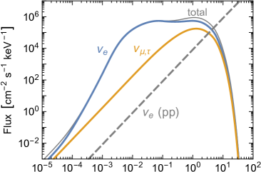
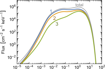
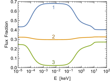
Figure 12: Solar neutrino flux at Earth from thermal processes Vitagliano et al. (2017). The antineutrino flux is the same. Top: Flavor-eigenstate fluxes in the absence of oscillations. For comparison, we also show the low-energy tail from the nuclear pp reaction (dashed) which produces only $\nu_{e}$. Middle: Mass-eigenstate fluxes for $\nu_{i}$ with $i=1$, 2 or 3 as indicated. This is the relevant representation for the fluxes arriving at Earth. Bottom: Fractional mass-eigenstate fluxes.

Solar neutrinos arriving at Earth have decohered into mass eigenstates. They are produced in the solar interior, where according to Eq. (70) the weak potential caused by electrons is $V_{e}=\sqrt{2}G_{\rm F}n_{e}\sim 7.8\times 10^{-12}~{}{\rm eV}$ near the solar center. Comparing with $\delta m^{2}/2E=3.7\times 10^{-8}~{}{\rm eV}~{}({\rm keV}/E)$ reveals that the matter effect is negligible for sub-keV neutrinos, in agreement with the discussion in Appendix C. Therefore, we can use the vacuum probabilities for a given flavor neutrino to be found in any of the mass eigenstates.

Specifically, from the top row of Eq. (64), we use the best-fit probabilities for a $\nu_{e}$ or $\overline{\nu}_{e}$ to show up in a given mass eigenstates to be $P_{e1}=0.681$, $P_{e2}=0.297$, and $P_{e3}=0.022$, which add up to unity. These probabilities apply to vector-current processes which produce almost pure $\nu_{e}\overline{\nu}_{e}$, whereas the axial-current processes, with equal $C_{\rm A}^{2}$ for all flavors, can be thought of as producing an equal mixture of pairs of mass eigenstates. In this way we find the mass-eigenstate fluxes at Earth shown in the middle panel of Fig. 12 and the corresponding fractional fluxes in the bottom panel.

Integrating over energies implies a total flux, number density, and energy density at Earth of neutrinos plus antineutrinos of all flavors

$$\Phi_{\nu\overline{\nu}} = 6.2\times 10^{6}~{}{\rm cm}^{-2}~{}{\rm s}^{-1},$$ (24a)

$$n_{\nu\overline{\nu}} = 2.1\times 10^{-4}~{}{\rm cm}^{-3},$$ (24b)

$$\rho_{\nu\overline{\nu}} = 507~{}{\rm meV}~{}{\rm cm}^{-3},$$ (24c)

implying $\langle E_{\nu}\rangle=\langle E_{\overline{\nu}}\rangle=2.46~{}{\rm keV}$. In analogy to traditional solar neutrinos, the flux and density changes by $\pm 3.4\%$ over the year due to the ellipticity of the Earth orbit. The local energy density in thermal solar neutrinos is comparable to the energy density of the CMB for massless cosmic neutrinos.

V.3 Very low energies

Thermal solar neutrinos appear to be the dominant flux at Earth for sub-keV energies all the way down to the CNB and the BBN neutrinos discussed in Secs. II and III. Therefore, it is useful to consider the asymptotic behavior at very low energies. For $E\lesssim 100$ meV, bremsstrahlung emission dominates which generically scales as $E^{2}$ at low energies Vitagliano et al. (2017). A numerical integration over the Sun provides the low-energy flux at Earth from bremsstrahlung for either $\nu$ or $\overline{\nu}$

$$\frac{d\Phi_{\nu}}{dE}=\frac{d\Phi_{\overline{\nu}}}{dE}=\frac{7.4\times 10^{6}}{{\rm cm}^{2}~{}{\rm s}~{}{\rm keV}}\,\left(\frac{E}{{\rm keV}}\right)^{2}.$$ (25)

The fractions in the mass eigenstates 1, 2, and 3 are 0.432, 0.323, and 0.245, corresponding to the low-energy plateau in the bottom panel of Fig. 12 and that were already shown in the BBN-context in Eq. (13). As explained by Vitagliano et al. (2017), bremsstrahlung produces an almost pure $\nu_{e}\bar{\nu}_{e}$ flux by the vector-current interaction which breaks down into mass eigenstates according to the vacuum-mixing probabilities given in the top row of Eq. (64). Moreover, bremsstrahlung produces all flavors equally by the axial-vector interaction. Adding the vector (28.4%) and axial-vector (71.6%) contributions provides these numbers.

One consequence of the relatively small bremsstrahlung flux is that there is indeed a window of energies between the CNB and very-low-energy solar neutrinos where the BBN flux of Sec. III dominates.

Of course, for energies so low that the emitted neutrinos are not relativistic, this result needs to be modified. For bremsstrahlung, the emission spectrum is determined by phase space, so $d\dot{n}=A\,p^{2}dp=A\,pE\,dE$ with $A$ some constant. For the flux of emitted neutrinos, we need a velocity factor $v=p/E$, so overall $d\Phi_{\nu}/dE\propto(E^{2}-m_{\nu}^{2})$ for $E\geq m_{\nu}$ and zero otherwise. The local density at Earth, on the other hand, does not involve $p/E$ and so is $dn_{\nu}/dE\propto E\sqrt{E^{2}-m_{\nu}^{2}}$.

VI Geoneutrinos

The decay of long-lived natural radioactive isotopes in the Earth, notably ²³⁸U, ²³²Th and ⁴⁰K, produce an MeV-range $\overline{\nu}_{e}$ flux exceeding $10^{25}~{}{\rm s}^{-1}$ Marx and Menyhárd (1960); Marx (1969); Eder (1966); Krauss et al. (1984); Fiorentini et al. (2007); Ludhova and Zavatarelli (2013); Bellini et al. (2013); Dye (2012); Smirnov (2019). As these “geoneutrinos” are actually antineutrinos they can be detected despite the large solar neutrino flux in the same energy range. The associated radiogenic heat production is what drives much of geological activity such as plate tectonics or vulcanism. The abundance of radioactive elements depends on location, in principle allowing one to study the Earth’s interior with neutrinos, although existing measurements by KamLAND and Borexino remain sparse.

VI.1 Production mechanisms

Geoneutrinos are primarily $\bar{\nu}_{e}$ produced in decays of radioactive elements with lifetime comparable to the age of the Earth, the so-called heat producing elements (HPEs) Ludhova and Zavatarelli (2013); Smirnov (2019). Geoneutrinos carry information on the HPE abundance and distribution and constrain the fraction of radiogenic heat contributing to the total surface heat flux of 50 TW. In this way, they provide indirect information on plate tectonics, mantle convection, magnetic-field generation, as well as the processes that led to the Earth formation Ludhova and Zavatarelli (2013); Bellini et al. (2013).

Around 99% of radiogenic heat comes from the decay chains of ²³²Th, ²³⁸U and ⁴⁰K. The main reactions are Fiorentini et al. (2007)

$$\kern-20.00003pt^{238}\mathrm{U} \rightarrow {}^{206}\mathrm{Pb}+8\alpha+8e+6\overline{\nu}_{e}+51.7\ \mathrm{MeV},$$ (26a)

$$\kern-20.00003pt^{232}\mathrm{Th} \rightarrow {}^{208}\mathrm{Pb}+6\alpha+4e+4\overline{\nu}_{e}+42.7\ \mathrm{MeV},$$ (26b)

$$\kern-20.00003pt^{40}\mathrm{K} \rightarrow {}^{40}\mathrm{Ca}+e+\overline{\nu}_{e}+1.31\ \mathrm{MeV}\ (89.3\%),$$ (26c)

$$\kern-20.00003pte+{}^{40}\mathrm{K} \rightarrow {}^{40}\mathrm{Ar}^{*}+\nu_{e}+0.044\ \mathrm{MeV}\ (10.7\%).$$ (26d)

The contribution from ²³⁵U is not shown because of its small isotopic abundance. Electron capture on potassium is the only notable $\nu_{e}$ component, producing a monochromatic 44 keV line. Notice that it is followed by the emission of a 1441 keV $\gamma$-ray to the ground state of ${}^{40}{\rm Ar}$. For the other reactions in Eq. (26) the average energy release in neutrinos is 3.96, 2.23 and 0.724 MeV per decay respectively Enomoto (2005), while the remainder of the reaction energy shows up as heat. An additional 1% of the radiogenic heat comes from decays of ⁸⁷Rb, ¹³⁸La and ¹⁷⁶Lu Ludhova and Zavatarelli (2013).

The geoneutrino spectra produced in these reactions, extending up to 3.26 MeV Ludhova and Zavatarelli (2013), depend on the possible decay branches and are shown in Fig. 13. The main detection channel is inverse beta decay $\overline{\nu}_{e}+p\to n+e^{+}$ with a kinematical threshold of 1.806 MeV (vertical dashed line in Fig. 13), implying that the large flux from ⁴⁰K is not detectable Bellini et al. (2013). On the other hand, a large fraction of the heat arises from the uranium and thorium decay chains. The resulting average flux is $\Phi_{\overline{\nu}_{e}}\simeq 2\times 10^{6}~{}{\rm cm}^{-2}~{}{\rm s}^{-1}$, comparable with the solar $\nu_{e}$ flux from ⁸B decay. However, detecting geoneutrinos is more challenging because of their smaller energies.

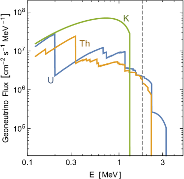
Figure 13: Average geoneutrino flux ($\overline{\nu}_{e}$ before flavor conversion) from the main production chains, assuming the BSE model of the Earth Enomoto (2005). The vertical dashed line marks the threshold of 1.806 MeV for inverse beta decay.

The differential $\overline{\nu}_{e}$ geoneutrino flux at position $\vec{r}$ on Earth is given by the isotope abundances $a_{i}(\vec{r}^{\,\prime})$ for any isotope $i$ at the position $\vec{r}^{\,\prime}$ and integrating over the entire Earth provides the expression Fiorentini et al. (2007); Smirnov (2019)

$$\Phi_{\overline{\nu}_{e}}(E,\vec{r})=\sum_{i}A_{i}\frac{dn_{i}}{dE}\!\int_{\oplus}\!\!d^{3}\vec{r}^{\,\prime}\frac{a_{i}(\vec{r}^{\,\prime})\rho(\vec{r}^{\,\prime})P_{ee}(E,|\vec{r}-\vec{r}^{\,\prime}|)}{4\pi|\vec{r}-\vec{r}^{\,\prime}|^{2}}.$$ (27)

Here $dn_{i}/dE$ is the $\overline{\nu}_{e}$ energy spectrum for each decay mode, $A_{i}$ the decay rate per unit mass, $\rho(\vec{r})$ the rock density, and $P_{ee}$ the $\overline{\nu}_{e}$ survival probability, where we have neglected matter effects so that $P_{ee}$ depends only on the distance between production and detection points.

To evaluate this expression one needs to know the absolute amount and distribution of HPEs. Although the crust composition is relatively well known, the mantle composition is quite uncertain Fiorentini et al. (2007); Bellini et al. (2013). Usually, the signal from HPEs in the crust is computed on the basis of the total amount of HPEs coming from the bulk silicate Earth (BSE) model, i.e., the model describing the Earth region outside its metallic core McDonough and Sun (1995); Palme and O’Neill (2003); then the corresponding amount of elements in the mantle is extrapolated. The content of elements in the Earth mantle can be estimated on the basis of cosmochemical arguments, implying that abundances in the deep layers are expected to be larger than the ones in the upper samples.

Given their chemical affinity, the majority of HPEs are in the continental crust. This is useful as most of the detectors sensitive to geoneutrinos are on the continents and the corresponding event rate is dominated by the Earth contribution. Usually the continental crust is further divided in upper, lower and middle continental crust. Among existing detectors, Borexino is placed on the continental crust in Italy Caminata et al. (2018); Agostini et al. (2020a), while KamLAND is in a complex geological structure around the subduction zone Gando et al. (2013); Shimizu (2017). An example for a global map of the expected $\overline{\nu}_{e}$ flux is shown in Fig. 14.

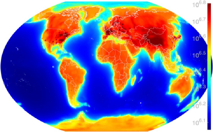
Figure 14: Global map of the expected $\overline{\nu}_{e}$ flux (in ${\rm cm}^{-2}~{}{\rm s}^{-1}$) of all energies from U and Th decays in the Earth and from reactors. The hot spots in the Eastern US, Europe and Japan are caused by nuclear power reactors. Credits: Antineutrino Global Map 2015 Usman et al. (2015) licensed under Creative Commons Attribution 4.0 International License.

VI.2 Earth modeling

The Earth was created by accretion from undifferentiated material. Chondritic meteorites seem to resemble this picture as for composition and structure. The Earth can be divided in five regions according to seismic data: core, mantle, crust (continental and oceanic), and sediment. The mantle is solid, but is affected by convection that causes plate tectonics and earthquakes Ludhova and Zavatarelli (2013).

Seismology has shown that the Earth is divided into several layers that can be distinguished by sound-speed discontinuities. Although seismology allows us to reconstruct the density profile, it cannot determine the composition. The basic structure of the Earth’s interior is defined by the one-dimensional seismological profile dubbed Preliminary Reference Earth Model (PREM), which is the basis for the estimation of geoneutrino production in the mantle Dziewonski and Anderson (1981). Meanwhile, thanks to seismic tomography, a three-dimensional view of the mantle structure has become available, for example Laske et al. (2012) and Pasyanos et al. (2014), but differences with respect to the 1D PREM are negligible for geoneutrino estimation Fiorentini et al. (2007).

As discussed in the previous section, uranium and thorium are the main HPEs producing detectable geoneutrinos. After the metallic core of the Earth separated, the rest of the Earth consisted of a homogeneous primitive mantle mainly composed of silicate rocks that then led to the formation of the present mantle and crust.

The outer layer is a thin crust which accounts for 70% of geoneutrino production Fiorentini et al. (2007); Šrámek et al. (2016). The crust probably hosts about half of the total uranium. The lithophile elements (uranium and thorium) tend to cluster in liquid phase and therefore concentrate in the crust, which is either oceanic or continental Enomoto (2005). The former is young and less than 10 km thick. The latter is thicker, more heterogeneous, and older that the oceanic counterpart. The crust is vertically stratified in terms of its chemical composition and is heterogeneous. The HPEs are distributed both in the crust and mantle. The geoneutrino flux strongly depends on location. In particular, the continental crust is about one order of magnitude richer in HPEs than the oceanic one. The continental crust is 0.34% of the Earth’s mass, but contains $40\%$ of the U and Th budget Bellini et al. (2013); Huang et al. (2013).

The mantle, which consists of pressurized rocks at high temperature, can be divided in upper and lower mantle Fiorentini et al. (2007). However, seismic discontinuities between the two parts do not divide the mantle into layers. We do not know whether the mantle moves as single or multiple layers, its convection dynamics, and whether its composition is homogeneous or heterogeneous. The available data are scarce and are restricted to the uppermost part.

Two models have been proposed Hofmann (1997). One is a two-layer model with a demarcation surface and a complete insulation between the upper mantle (poor in HPEs) and the lower layer. Another one is a fully mixed model, which is favored by seismic tomography. Concerning the estimation of the related geoneutrino flux, both models foresee the same amount of HPEs, but with different geometrical distributions Mantovani et al. (2004); Enomoto et al. (2005). In the following, we assume a homogeneous distribution of U and Th in the mantle. Geophysicists have proposed models of mantle convection predicting that 70% of the total surface heat flux is radiogenic. Geochemists estimate this figure to be 25%; so the spread is large Bellini et al. (2013); Meroni and Zavatarelli (2016).

The Earth’s innermost part is the core, which accounts for 32% of the Earth’s mass, and is made of iron with small amounts of nickel Fiorentini et al. (2007). Because of their chemical affinity, U and Th are believed to be absent in the core.

BSE models adopted to estimate the geoneutrino flux fall into three classes: geochemical, geodynamical, and cosmochemical Ludhova and Zavatarelli (2013). Geochemical models are based on the fact that the composition of carbonaceous chondrites matches the solar photospheric abundances of refractory lithophile and siderophile elements. A typical bulk-mass Th/U ratio is 3.9. Geodynamical models look at the amount of HPEs needed to sustain mantle convection. Cosmochemical models are similar to geochemical ones, but assume a mantle composition based on enstatite chondrites and yield a lower radiogenic abundance.

A reference BSE model to estimate the geoneutrino production is the starting point for studying the expectations and potential of various neutrino detectors. It should incorporate the best available geochemical and geophysical information. The geoneutrino flux strongly depends on location, so the global map shown in Fig. 14 is only representative. It includes the geoneutrino flux from the U and Th decay chains as well as the reactor neutrino flux Usman et al. (2015).

A measurement of the geoneutrino flux could be used to estimate our planet’s radiogenic heat production and to constrain the composition of the BSE model. A leading BSE model McDonough and Sun (1995) predicts a radiogenic heat production of 8 TW from ${}^{238}\mathrm{U}$, 8 TW from ${}^{232}\mathrm{Th}$, and 4 TW from ${}^{40}\mathrm{K}$, together about half the heat dissipation rate from the Earth’s surface. According to measurements in chondritic meteorites, the concentration mass ratio Th/U is 3.9. Currently, the uncertainties on the neutrino fluxes are as large as the predicted values.

The neutrino event rate is often expressed in Terrestrial Neutrino Units (TNUs), i.e., the number of interactions detected in a target of $10^{32}$ protons (roughly correspondent to 1 kton of liquid scintillator) in one year with maximum efficiency Ludhova and Zavatarelli (2013). So the neutrino event rates can be expressed as

$${}^{232}\mathrm{Th} S=4.07~{}\mathrm{TNU}\times\Phi_{\overline{\nu}_{e}}\big{/}10^{6}\,{\rm cm}^{-2}\,{\rm s}^{-1}$$ (28a)

$${}^{238}\mathrm{U~{}} S=12.8~{}\mathrm{TNU}\times\Phi_{\overline{\nu}_{e}}\big{/}10^{6}\,{\rm cm}^{-2}\,{\rm s}^{-1}$$ (28b)

for the thorium and uranium decay chains.

VI.3 Detection opportunities

Geoneutrinos were first considered in 1953 to explain a puzzling background in the Hanford reactor neutrino experiment of Reines and Cowan, but even Reines’ generous estimate of $10^{8}~{}{\rm cm}^{-2}~{}{\rm s}^{-1}$ fell far short (the real explanation turned out to be cosmic radiation). First realistic geoneutrino estimates appeared in the 1960s by Marx and Menyhárd (1960) and Marx (1969) and independently by Eder (1966), to be followed in the 1980s by Krauss et al. (1984).

The first experiment to report geoneutrino detection was KamLAND in 2005, a 1000 t liquid scintillator detector in the Kamioka mine Araki et al. (2005a). The detection channel is inverse beta decay (IBD), $\bar{\nu}_{e}+p\to n+e^{+}$, using delayed coincidence between the prompt positron and a delayed $\gamma$ from neutron capture. The results were based on 749.1 live days, corresponding to an exposure of $(0.709\pm 0.035)\times 10^{32}~{}{\rm protons}\times{\rm year}$, providing 152 IBD candidates, of which $25^{+19}_{-18}$ were attributed to geo-$\bar{\nu}_{e}$. This signal corresponds to about one geoneutrino per month to be distinguished from a background that is five times larger. About $80.4\pm 7.2$ of the background events were attributed to the $\bar{\nu}_{e}$ flux from nearby nuclear reactors — KamLAND was originally devised to detect flavor oscillations of reactor neutrinos (Sec. VII).

Over the years, the detector was improved, notably by background reduction through liquid-scintillator purification. A dramatic change was the shut-down of the Japanese nuclear power reactors in 2011 following the Fukushima Daiichi nuclear disaster (March 2011). For KamLAND this implied a reactor-off measurement of backgrounds and geoneutrinos that was included in the latest published results, based on data taken between March 9, 2002 and November 20, 2012 Gando et al. (2013). Preliminary results from data taken up to 2016, including 3.5 years of a low-reactor period (and of this 2.0 years reactor-off), were shown at a conference in October 2016 Watanabe (2016) and also reported in a recent review article Smirnov (2019). We summarize these latest available measurements in Table 3.

Table 3: Geoneutrino observations. The Th/U abundance ratio is assumed to be the chondritic value.

	KamLAND	Borexino
Period	2002–2016	2007–2019
Live days	3900.9	3262.74
Exposure	$6.39$	$1.29\pm 0.05$
($10^{32}$ protons$\times$year)
IBD Candidates	1130	154
Reactor $\bar{\nu}_{e}$	$618.9\pm 33.8$	$92.5^{+12.2}_{-9.9}$
Geoneutrinos (68% C.L.)
Number of $\bar{\nu}_{e}$	139–192	43.6–62.2
Signal (TNU)	29.5–40.9	38.9–55.6
Flux ($10^{6}~{}{\rm cm}^{-2}~{}{\rm s}^{-1}$)	3.3–4.6	4.8–6.2

A second experiment that has detected geoneutrinos is Borexino, a 300 t liquid scintillator detector in the Gran Sasso National Laboratory in Italy, reporting first results in 2010 Caminata et al. (2018). Despite its smaller size, Borexino is competitive because of its scintillator purity, large underground depth, and large distance from nuclear power plants, effects that all help to reduce backgrounds. Comprehensive results for the data-taking period December 2007–April 2019 were recently published Agostini et al. (2020a) and are summarized in Table 3.

Reactor neutrinos (Sec. VII) are the main background for geoneutrino detection, whereas atmospheric neutrinos and the diffuse supernova neutrino background (Sec. IX) are negligible. Other spurious signals include intrinsic detector contamination, cosmogenic sources, and random coincidences of non-correlated events. While the reactor flux at Borexino is usually much smaller than at KamLAND, the shut-down of the Japanese reactors has changed this picture for around 1/3 of the KamLAND live period. From Table 3 we conclude that at Borexino, the reactor signal was around 1.7 times the geoneutrino signal, whereas at KamLAND this factor was on average around 3.7. Any of these $\bar{\nu}_{e}$ measurements refer to the respective detector sites and include the effect of flavor conversion on the way between source and detector.

The overall results in Table 3 assume a Th/U abundance ratio fixed at the chondritic value of 3.9, but both Borexino and KamLAND provide analyses with independent contributions. For example, KamLAND finds for the ratio $4.1^{+5.5}_{-3.3}$, consistent with the simplest assumption but with large uncertainties Watanabe (2016). KamLAND is also beginning to discriminate between the geodynamical, geochemical and cosmochemical BSE models, somewhat disfavoring the latter. The radiogenic heat production is allowed to be roughly in the range 8–30 TW. Borexino finds a measured mantle signal of $21.2^{+9.5}_{-9.0}({\rm stat})^{+1.1}_{-0.9}({\rm sys})$ TNU, corresponding to the production of a radiogenic heat of $24.6^{+11.1}_{-10.4}$ TW (68% interval) from ²³⁸U and ²³²Th in the mantle. Assuming 18% contribution of ⁴⁰K in the mantle and $8.1^{+1.9}_{-1.4}$ TW of the total radiogenic heat of the lithosphere, Borexino estimates the total radiogenic heat of the Earth to be $38.2^{+13.6}_{-12.7}$ TW Agostini et al. (2020a). Overall, while the observation of geoneutrinos in these two detectors is highly significant, detailed geophysical conclusions ultimately require better statistics.

Several experiments, in different stages of development, will improve our knowledge. For example, SNO+ in Canada expects a geoneutrino rate of 20/year Arushanova and Back (2017). The site is in the old continental crust containing felsic rocks which are rich in U and Th. The crust at the SNO+ location is especially thick, about 40% more than at Gran Sasso and Kamioka. JUNO in China also plans to measure geoneutrinos. Finally, the Hanohano project has been proposed in Hawaii, a 5 kton detector on the oceanic crust Cicenas and Solomey (2012). Because the oceanic crust is thin, 75% of the signal would come from the mantle.

VII Reactor Neutrinos

Nuclear power plants release a few percent of their energy production in the form of MeV-range $\overline{\nu}_{e}$ arising from the decay of fission products. In contrast to other human-made neutrino sources such as accelerators, reactors produce a diffuse flux that can dominate over geoneutrinos in entire geographic regions and are therefore a legitimate GUNS component. Historically, reactor neutrinos were fundamental to the study of neutrino properties, including their very first detection by Cowan and Reines in the 1950s, and they remain topical for measuring neutrino mixing parameters and possible sterile states Giunti and Kim (2007); Tanabashi et al. (2018); Qian and Peng (2019), as well as for many applied fields Bergevin et al. (2019).

VII.1 Production and detection of reactor neutrinos

Nuclear power plants produce $\overline{\nu}_{e}$’s through $\beta$-decays of neutron-rich nuclei. The main contributions come from the fission of ${}^{235}\rm U$ (56%), ${}^{239}\rm Pu$ (30%), ${}^{238}\rm U$ (8%) and ${}^{241}\rm Pu$ (6%), where the percentages vary over time and we reported typical values of fission fractions during operation Giunti and Kim (2007); Baldoncini et al. (2015). In addition, below the detection threshold of inverse beta decay $E_{\rm min}=1.8~{}\rm MeV$ there is another $\overline{\nu}_{e}$ source due to neutron captures. The most important is the decay of ${}^{239}\rm U$ produced by the neutron capture on ${}^{238}\mathrm{U}$, which is usually written as ${}^{238}\mathrm{U}(n,\gamma)^{239}\rm U$. To obtain a basic estimate of the $\overline{\nu}_{e}$ flux from a reactor we note that on average a fission event releases about 6 neutrinos and a total energy of about $200~{}\rm MeV$. A nuclear power plant producing $1~{}\rm GW$ of thermal power will then produce a $\overline{\nu}_{e}$ flux of $2\times 10^{20}~{}\rm s^{-1}$ Giunti and Kim (2007).

The globally installed nuclear power corresponds to around 0.4 TW electric or, with a typical efficiency of 33%, to 1.2 TW thermal. This is a few percent of the natural radiogenic heat production in the Earth, so the overall reactor neutrino flux is only a few percent of the geoneutrino flux, yet the former can dominate in some geographic regions and has a different spectrum.

Predicting the spectrum is a much more complicated task as many different decay branches must be included. In the last 50 years, two main approaches were used. One method predicts the time dependent total flux by summing over all possible $\beta$-decay branches, but the spectrum is very uncertain because the fission yields and endpoint energies are often not well known, one needs a good model for the Coulomb corrections entering the Fermi function, and so forth. The alternative is to use the measured electron spectrum for different decay chains, which can be inverted taking advantage of the relation

$$E_{\nu}=E_{e}+T_{n}+m_{n}-m_{p}\simeq E_{e}+1.293~{}\rm MeV\,,$$ (29)

where $T_{n}$ is the small recoil kinetic energy of the neutron and $E_{e}$ is the energy of the outgoing positron.

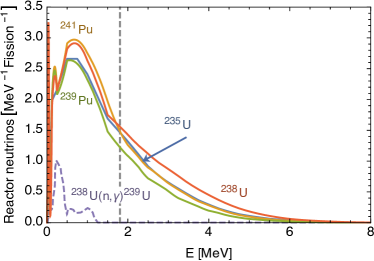
Figure 15: The $\overline{\nu}_{e}$ energy spectra for ${}^{235}\rm U$, ${}^{238}\rm U$, ${}^{239}\rm Pu$, and ${}^{241}\rm Pu$ fissions. The inverse beta decay threshold is marked by a vertical dashed line. At low energies, the dominant contribution is due to neutron capture processes ${}^{238}\mathrm{U}(n,\gamma)^{239}\rm U$, here rescaled by a factor $1/20$.

Until 2011, the standard results were the ones obtained by Vogel and Engel (1989), but then two papers recalculated the spectrum at energies larger than 2 MeV with different methods, one by Huber (2011) and one by Mueller et al. (2011). Figure 15 shows the spectrum due to the dominant processes reported in Table II of Vogel and Engel (1989) for energies smaller than 2 MeV, while for larger energies we use Tables VII–IX of Huber (2011) for ${}^{235}\rm U$, ${}^{239}\rm Pu$ and ${}^{241}\rm Pu$ and Table III of Mueller et al. (2011) for ${}^{238}\rm U$; finally, the low-energy spectrum of neutron capture ${}^{238}\mathrm{U}(n,\gamma)^{239}\rm U$ are directly extracted from Qian and Peng (2019). Notice that fits to the tables are reported in these references.

The detection of reactor neutrinos typically relies on inverse beta decay on protons, $\overline{\nu}_{e}+p\to n+e^{+}$. The cross section is usually expressed in terms of well measured quantities such as the neutron lifetime $\tau_{n}$ and the electron mass $m_{e}$ Vogel and Beacom (1999),

$$\sigma_{\mathrm{CC}}^{\overline{\nu}_{e}p}=\frac{2\pi^{2}}{\tau_{n}m_{e}^{5}f}E_{e}\sqrt{E_{e}^{2}-m_{e}^{2}}\,.$$ (30)

Here $f$ is the dimensionless phase-space integral

$$f=\int_{m_{e}}^{m_{n}-m_{p}}\!\!dE_{e}\frac{(m_{n}-m_{p}-E_{e})^{2}E_{e}\sqrt{E_{e}^{2}-m_{e}^{2}}}{m_{e}^{5}}\,,$$ (31)

where we neglect the small neutron recoil energy. The detection signature features a prompt signal due to the positron, followed by neutron capture. Alternatives to this process include charged and neutral current deuteron break-up using heavy water, $\overline{\nu}$-$e$ elastic scattering, and coherent $\overline{\nu}$-nucleus interactions Giunti and Kim (2007).

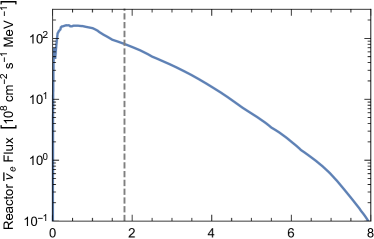
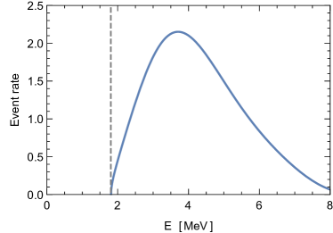
Figure 16: Typical reactor neutrino spectrum, here from the Japanese experimental fast reactor JOYO Furuta et al. (2012). Top: Flux at a distance of 24.3 m. Bottom: Event rate (arbitrary units) as a function of neutrino energy, i.e., the neutrino energy distribution folded with the interaction cross section for inverse $\beta$ decay. Only $\overline{\nu}_{e}$ above the threshold of 1.8 MeV (vertical dashed line) are detectable. The event rate peaks at $E_{\nu}\sim 4~{}{\rm MeV}$.

As a typical example we show in Fig. 16 (top) the flux from the Japanese experimental fast reactor JOYO Furuta et al. (2012), which has 140 MW thermal power and a detector at the close distance of 24.3 m. Convolution with the inverse $\beta$ cross section (bottom panel) shows that the interactions peak for $E_{\overline{\nu}_{e}}\sim 4~{}{\rm MeV}$. While the quantitative details strongly depend on the reactor and detector, several general features can be pointed out Giunti and Kim (2007). First, the large threshold implies that only reactions with large Q-value can be observed, so only one fourth of the total flux can be detected. Another important point is that reactor shutdowns can be used to measure background and that the intensity of the flux is proportional to the thermal power, which is accurately monitored. Moreover, the flux is very large, so the detectors do not need large shielding against cosmic rays. All of these advantages make reactor neutrinos a fundamental tool for measuring intrinsic neutrino properties such as mixing angles and mass differences.

The global flux is produced by around 500 reactors worldwide with a very uneven geographic distribution. In Fig. 17 we show a global map, restricted to the very narrow energy range 3.00–3.01 MeV, allowing one to discern flavor oscillations over 100 km distances. The three main centers of production are the Eastern US, Europe, and East Asia, notably Japan.

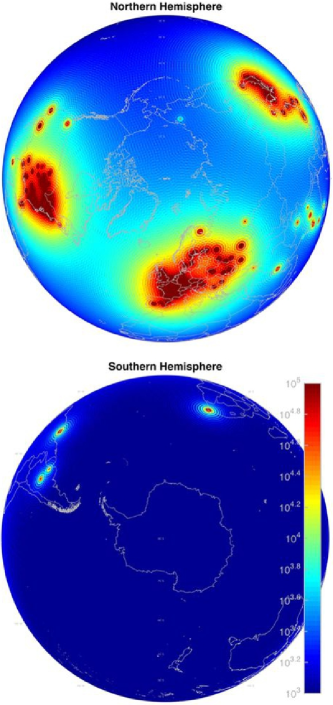
Figure 17: Global map of the expected $\overline{\nu}_{e}$ flux (in $1/100\,{\rm cm}^{2}/{\rm s}$) in the narrow energy range 3.00–3.01 MeV from all power reactors. Flavor oscillations driven by the “solar” mixing parameters are visible on the 100 km scale. Figure credit: Antineutrino Global Map 2015 Usman et al. (2015) licensed under Creative Commons Attribution 4.0 International License.

VII.2 Measurements

While we have included reactor neutrinos in our discussion of the diffuse neutrino background at Earth, of course reactors, or clusters of reactors, are typically used as nearby sources to study neutrino properties. Reactor experiments were the first successful attempt to detect the elusive neutrinos. The proposal of using inverse beta decay dates back to Bethe and Peierls Bethe and Peierls (1934), but it was only in 1953 that Reines and Cowan started their experiments at Hanford and Savanah River which eventually detected neutrinos for the first time Cowan et al. (1953). Nuclear power plants have been employed in the following decades to study neutrino properties many times.

Concerning flavor conversion, a mile-stone discovery was the detection of $\overline{\nu}_{e}$ disappearance by KamLAND in 2002 over an approximate distance of 180 km Eguchi et al. (2003), driven by the “solar” mixing parameters $\theta_{12}$ and $\delta m^{2}$. The subsequent measurement of a spectral distortion Araki et al. (2005b) revealed first direct evidence for the phenomenon of flavor oscillations with the usual energy dependence. Notice that matter effects are here subdominant, so essentially one is testing vacuum oscillations.

The earlier search over much shorter distances for oscillations driven by the mixing angle $\theta_{13}$ and the “atmospheric” mass difference $\Delta m^{2}$ by the CHOOZ Apollonio et al. (1999) and Palo Verde Boehm et al. (2001) experiments proved elusive. However, since 2012, a new generation of reactor experiments (Double Chooz Abe et al. (2012), Daya Bay An et al. (2012), and RENO Ahn et al. (2012)) has succeeded to measure a non-zero value for $\theta_{13}$ with high precision.

The frontier of reactor neutrino measurements will be advanced by the JUNO detector An et al. (2016) that is currently under construction in China. One of the prime goals is to detect subtle three-flavor interference effects at an approximate distance of 60 km to establish the neutrino mass ordering.

Meanwhile, the “reactor antineutrino anomaly” Mention et al. (2011) remains unsettled, i.e., a few-percent deficit of the measured $\overline{\nu}_{e}$ flux at very close distances from reactors. Other anomalies include $\overline{\nu}_{e}$ appearance and $\nu_{e}$ disappearance, see Böser et al. (2020) and references therein. One interpretation are oscillations to sterile neutrinos driven by an eV-scale mass difference Conrad and Shaevitz (2018); Giunti and Lasserre (2019). Recent antineutrino flux predictions Estienne et al. (2019); Hayen et al. (2019) have been used to reevaluate the significance of the reactor anomaly; in the ratios of measured antineutrino spectra an anomaly may still persist Berryman and Huber (2020).

VIII Supernova neutrinos

The core collapse of a massive star within a few seconds releases the gravitational binding energy of a neutron star (NS), $E_{\rm b}\sim 3\times 10^{53}~{}{\rm erg}$, in the form of neutrinos in what is known as a supernova (SN) explosion. This energy release is roughly comparable to that of all stars in the Universe within the same period. While the neutrino burst from the next nearby SN is one of the most cherished targets of neutrino astronomy, it is a transient signal and thus not part of the GUNS. We here summarize the main features of core-collapse neutrino emission primarily as an ingredient for the diffuse SN neutrino background (DSNB) presented in Sec. IX. For reviews of SN neutrinos see Janka (2012), Scholberg (2012), Mirizzi et al. (2016), and Janka et al. (2016).

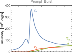
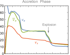
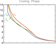
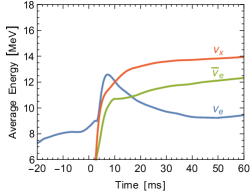
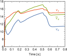
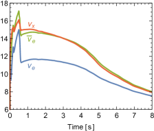
Figure 18: Luminosities and average energies for $\nu_{e}$, $\overline{\nu}_{e}$ and $\nu_{x}$ (representing any of $\nu_{\mu}$, $\overline{\nu}_{\mu}$, $\nu_{\tau}$ or $\overline{\nu}_{\tau}$) for the main phases of neutrino emission from a core-collapse SN. From left to right: (1) Infall, bounce and initial shock-wave propagation, including prompt $\nu_{e}$ burst. (2) Accretion phase with significant flavor differences of fluxes and spectra. (3) Cooling of the proto neutron star (PNS), only small flavor differences between fluxes and spectra. Based on a spherically symmetric $27\,M_{\odot}$ Garching model with explosion triggered by hand during 0.5–0.6 s. It uses the nuclear equation of state of Lattimer and Swesty with nuclear incompressibility modulus $K=220$ MeV and includes a mixing-length treatment of PNS convection. The final gravitational mass is $1.592\,M_{\odot}$ (or 89.6% of the baryonic mass of $1.776\,M_{\odot}$), so the mass deficit is $E_{\rm b}=0.184\,M_{\odot}=3.31\times 10^{53}~{}{\rm erg}$ that was lost in neutrinos. See the Garching Core-Collapse Supernova Data Archive at https://wwwmpa.mpa-garching.mpg.de/ccsnarchive/ for several suites of SN models.

VIII.1 Generic features of supernova neutrinos

At the end of its life, the compact core of an evolved star becomes unstable and collapses to nuclear density, where the equation of state stiffens Janka (2012); Burrows (2013); Janka (2017). At this core bounce, a shock wave forms, moves outward, and ejects most of the mass in the form of a SN explosion, leaving behind a compact remnant that cools to become a NS. Typical masses are around $M_{\rm{NS}}\simeq 1.5\,M_{\odot}$, with $2\,M_{\odot}$ the largest observed case. The radius is $R_{\rm{NS}}\simeq 12$–$14$ km, the exact value and NS structure depending on the nuclear equation of state. Within these uncertainties one expects the release of the following binding energy

$$E_{\rm b}\simeq\frac{3}{5}\frac{G_{\rm N}M_{\rm{NS}}^{2}}{R_{\rm{NS}}}\simeq 3\times 10^{53}~{}{\rm erg}\simeq 2\times 10^{59}~{}{\rm MeV}\ ,$$ (32)

with $G_{\rm N}$ being Newton’s gravitational constant.

This huge amount of energy appears in the form of neutrinos because the interaction rate of $\gamma$ and $e^{\pm}$ is so large in dense matter that they contribute little to energy transfer, whereas gravitons interact far too weakly to be effective. Moreover, in hot nuclear matter the neutrino mean free path is short compared to the geometric dimension of the collapsed object, so $\nu$ and $\overline{\nu}$ of all flavors thermalize, for example by nucleon-nucleon bremsstrahlung and other processes Bruenn (1985). Hence, very approximately we may think of the collapsed SN core as a blackbody source for $\nu$ and $\overline{\nu}$ of all flavors.

The diffusion character of neutrino transport leads to an estimated time of a few seconds for most of the energy trapped in the SN core to escape. The emission temperature depends on radiative transfer in the decoupling region (“neutrino sphere”); typically $T_{\nu}\simeq 3$–$5$ MeV, i.e., average energies $\langle E_{\nu}\rangle=(3/2)\,T_{\nu}\simeq 10$–$15$ MeV after neutrino decoupling Janka (2012); Burrows (2013); Janka (2017). This scale is similar to that of solar and geoneutrinos, where however it is set by nuclear physics. Overall one expects the emission of around $E_{\rm b}/\langle E_{\nu}\rangle\simeq 3\times 10^{57}$ particles for each of the six $\nu$ and $\overline{\nu}$ species.

Besides energy, the SN core must also radiate lepton number (deleptonization). The final NS contains only a small proton (or electron) fraction, whereas the collapsing material, consisting of elements between O and Fe, initially has an electron fraction $Y_{e}=0.46$–$0.5$. A baryonic mass of $1.5\,M_{\odot}$ corresponds to $2\times 10^{57}$ nucleons, implying that $1\times 10^{57}$ units of electron lepton number must escape in the form of $\nu_{e}$, ignoring for now flavor conversion. Comparison with the estimated $6\times 10^{57}$ of $\nu_{e}$ plus $\overline{\nu}_{e}$ to be radiated by the required energy loss reveals a significant excess of $\nu_{e}$ over $\overline{\nu}_{e}$ emission Mirizzi et al. (2016).

The overall picture of neutrino energies and time scale of emission was confirmed on 23 February 1987 by the neutrino burst from SN 1987A in the Large Magellanic Cloud with a total of about two dozen events in three small detectors Hirata et al. (1987); Bionta et al. (1987); Alekseev et al. (1988). However, the data was too sparse for detailed quantitative tests. The next nearby SN would provide high statistics, especially in Super-Kamiokande, in IceCube, or in upcoming large detectors such as Hyper-Kamiokande or DUNE. The expected large number of neutrino events in these detectors may show detailed imprints of SN physics Scholberg (2018).

VIII.2 Reference neutrino signal

The standard paradigm of stellar core-collapse and SN explosions has evolved over decades of numerical modeling Janka (2012); Janka et al. (2016), first in spherical symmetry (1D) and over the past years with ever more refined 3D models. After the collapse has begun and when the density exceeds some $10^{12}~{}{\rm g}~{}{\rm cm}^{-3}$, neutrinos are entrained by the infalling matter because of coherent scattering on large nuclei. When nuclear density of $3\times 10^{14}~{}{\rm g}~{}{\rm cm}^{-3}$ is reached, the core bounces and a shock wave forms within the core at an enclosed mass of around $0.5\,M_{\odot}$. As the shock propagates outward, it loses energy by dissociating iron and eventually stalls at a radius of some 150 km, while matter keeps falling in. Meanwhile the neutrino flux streaming through this region deposits some of its energy, rejuvenating the shock wave, which finally moves on and ejects the outer layers. It leaves behind a hot and dense proto neutron star (PNS), which cools and deleptonizes within a few seconds. This is the essence of the neutrino-driven explosion mechanism, also called delayed explosion mechanism or Bethe-Wilson mechanism Bethe and Wilson (1985).

The corresponding neutrino signal falls into three main phases shown in Fig. 18, using a $27\,M_{\odot}$ spherically symmetric model for illustration. As in most simulations, neutrino radiative transfer is treated in a three-species approximation consisting of $\nu_{e}$, $\overline{\nu}_{e}$ and $\nu_{x}$ which stands for any of $\nu_{\mu}$, $\overline{\nu}_{\mu}$, $\nu_{\tau}$ and $\overline{\nu}_{\tau}$. This approach captures the main flavor dependence caused by charged-current interactions of the $e$-flavored states. However, heavy-flavor $\nu$ and $\overline{\nu}$ do not interact exactly the same because of recoil corrections and weak magnetism Horowitz and Pérez-García (2003). Moreover, the $\mu$ and $\tau$ flavored states differ by the presence of some muons ($m_{\mu}=105.7~{}{\rm MeV}$) in matter that reaches temperatures of several ten MeV Bollig et al. (2017).

Prompt Burst.—Soon after bounce, the shock wave breaks through the edge of the iron core, liberating the conspicuous prompt $\nu_{e}$ burst that corresponds to a significant fraction of the overall lepton number. It is therefore also called the deleptonization or neutronization or breakout burst. During the post-bounce time window $-20$ ms to 60 ms shown in the left panels in Fig. 18, the SN core radiates about 5% of the total energy that corresponds to the period shown in the rightmost panels, whereas it radiates $0.4\times 10^{57}$ units of lepton number, i.e., around 50% of what is emitted over the full period. The features of the prompt-burst phase are thought to be essentially universal Liebendörfer et al. (2003); Kachelrieß et al. (2005). The little dip in the $\nu_{e}$ luminosity curve at $t=0$–4 ms, for example, is explained by the shock first compressing matter to opaque conditions before the post-shock layer re-expands to become transparent.

Accretion Phase.—As the shock wave stalls, neutrino emission is powered by the accretion flow of matter onto the SN core, emitting $\nu_{e}$ and $\overline{\nu}_{e}$ with almost equal luminosities, but somewhat different average energies, so the $\nu_{e}$ particle flux is some 20% larger than the $\overline{\nu}_{e}$ one. The production and interaction is mostly by $\beta$ processes on protons and neutrons. Heavy-flavor $\nu$ and $\overline{\nu}$, on the other hand, are produced in pairs and emerge from somewhat deeper layers, with a smaller radiating region and therefore smaller fluxes. Their average energies, however, are very similar to that of $\overline{\nu}_{e}$. The large hierarchy of flavor-dependent average energies that was seen, for example, in the often-cited Livermore model Totani et al. (1998) is not physical Raffelt (2001) and is not borne out by present-day simulations. The luminosity drop at around 200 ms represents the infall of the Si/O interface, after which the accretion rate and luminosity become smaller. Over the entire accretion phase, the mass gain and concomitant contraction of the SN core show up in the increasing neutrino energies.

Explosion.—Spherically symmetric numerical models do not explode except for the smallest-mass progenitors, such as electron-capture supernovae Kitaura et al. (2006), so the duration of the accretion phase, and if an explosion occurs at all, can not be inferred from these models. For example, the explosion in the case of Fig. 18 was triggered by hand during the 500–600 ms period. Three-dimensional simulations successfully explode and suggest that the explosion time strongly depends on the SN model and may vary up to few hundreds of ms relative to what is shown in Fig. 18, see e.g. Bollig et al. (2017), Summa et al. (2018), Burrows et al. (2020), and Vartanyan et al. (2019). The quenching of accretion strongly reduces the $\nu_{e}$ and $\overline{\nu}_{e}$ luminosities which drop to the component provided by core emission.

Cooling.—The remaining evolution consists of cooling and deleptonization of the PNS. The luminosity is essentially equipartitioned among the six species, whereas $\langle E_{\nu_{e}}\rangle$ is smaller than the others, i.e., there is a net lepton number flux. The quantitative details depend strongly on the PNS mass and the nuclear equation of state, see e.g. Oertel et al. (2017), Nakazato and Suzuki (2019), and Nakazato and Suzuki (2020). Note that we show the neutrino signal until $8$ s in Fig. 18, but this is not a hard cut-off. We refer the reader to Nakazato et al. (2013) and Nakazato and Suzuki (2020) for discussions of late SN neutrino emission. The neutronization burst and the accretion phase release about $50\%$ of the total energy; the other half is emitted during the cooling phase.

The instantaneous neutrino spectra are quasi thermal, but do not follow exactly a Fermi-Dirac distribution. Rather they are “pinched,” i.e., the spread of energies around the mean is less than in the thermal case. Phenomenologically, the numerical spectra are well described by a Gamma distribution of the form Keil et al. (2003); Tamborra et al. (2012)

$$f(E)\propto\left(\frac{E}{E_{\rm av}}\right)^{\alpha}\exp\left[-\frac{(\alpha+1)E}{E_{\rm av}}\right]\,,$$ (33)

where $\alpha$ is the “pinching parameter” with $\alpha=2$ corresponding to a Maxwell-Boltzmann distribution. For any $\alpha$, the parameter $E_{\rm av}$ matches $\langle E\rangle$, whereas $\alpha$ is fixed to match, for example, $\langle E^{2}\rangle$ of the numerical spectrum by $\langle E^{2}\rangle/\langle E\rangle^{2}=(2+\alpha)/(1+\alpha)$. In addition, the overall normalization is fixed to match the numerical case. The pinching is largest for $\nu_{e}$, especially during the prompt burst, and smallest for $\nu_{x}$.

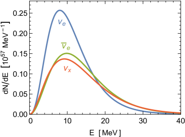
Figure 19: Time-integrated spectra of the reference model of Fig. 18. The total particle emission is $3.2\times 10^{57}~{}\nu_{e}$, $2.4\times 10^{57}~{}\overline{\nu}_{e}$, and $2.3\times 10^{57}$ for each of $\nu_{\mu}$, $\overline{\nu}_{\mu}$, $\nu_{\tau}$ or $\overline{\nu}_{\tau}$.

The time-integrated flux spectra of our reference model are shown in Fig. 19. They are superpositions of pinched spectra with different $E_{\rm av}$, which broadens their spectral shape, and therefore do not need to be pinched themselves. We find the average energies $\langle E_{\nu_{e}}\rangle=11.3~{}{\rm MeV}$, $\langle E_{\overline{\nu}_{e}}\rangle=13.9~{}{\rm MeV}$, and $\langle E_{\nu_{x}}\rangle=13.8~{}{\rm MeV}$, as well as the pinching parameters $\alpha_{\nu_{e}}=2.5$, $\alpha_{\overline{\nu}_{e}}=2.4$, and $\alpha_{\nu_{x}}=2.0$. So in this example, the integrated spectra follow nearly a Maxwell-Boltzmann distribution.

VIII.3 Electron-capture supernovae

Assuming this scenario to capture the main features of a SN neutrino signal, one still expects large case-by-case variations depending on progenitor properties. The lowest-mass SN progenitors (about 8–$10\,M_{\odot}$) become unstable due to electron capture before nuclear burning of their O-Ne-Mg core can be ignited, so they never reach an iron core. These “electron capture SNe” or “O-Ne-Mg-core SNe” could represent 30% of all cases because the initial mass function decreases rapidly with increasing mass. Spherically symmetric models of these low-mass progenitors explode after a very short accretion phase, but otherwise resemble what was shown earlier Fischer et al. (2010); Hüdepohl et al. (2010).

VIII.4 Failed explosions

For higher-mass progenitors, numerical models do not explode. It remains open if this question depends, for example, on quantitative details of neutrino energy transfer and 3D effects, on details of the progenitor models, or if a crucial piece of input physics is missing. Moreover, probably not all collapsing stellar cores lead to successful explosions — the class of failed SNe, leaving a black hole (BH) instead of a NS as a compact remnant. Using the “compactness parameter” as a criterion, recent theoretical work hints that up to 40% of all collapsing cores may lead to BH formation O’Connor and Ott (2011); Ertl et al. (2016); Sukhbold et al. (2016).

The cosmic star-formation rate predicts perhaps twice the observed SNe rate at high redshifts, suggesting a significant fraction of failed explosions Hopkins and Beacom (2006); Horiuchi et al. (2011). Likewise, the “red supergiant problem” suggests a cutoff of around $18\,M_{\odot}$ in the mass range of identified SN progenitors Smartt et al. (2009); Jennings et al. (2014). A significant fraction of failed SNe would also naturally explain the compact-object mass distribution Kochanek (2015). Motivated by these hints, a survey looks for disappearing red supergiants in 27 galaxies within 10 Mpc with the Large Binocular Telescope Adams et al. (2017). Over the first seven years, ending in early 2016, this survey found six core-collapse SNe and one candidate for a failed SN, providing $0.14_{-0.10}^{+0.33}$ for the fraction of failed SNe.

In the neutrino signal of a failed SN, the cooling phase would be missing, whereas the accretion phase would abruptly end. The average neutrino energies would increase until this point and the $\nu_{e}$ and $\overline{\nu}_{e}$ fluxes dominate Sumiyoshi et al. (2006); Nakazato et al. (2008); Walk et al. (2020). The overall emitted neutrino energy could exceed that of an exploding SN. The crucial point is that BH formation is delayed, not prompt, so the core bounce and shock scenario is crucial for the expected neutrino burst of both exploding and failed cases.

An intermediate class between exploding and failed progenitors are fallback SNe, where BH formation is delayed, if the explosion energy is not sufficient to unbind the star Fryer (2009); Wong et al. (2014). Hence, a fraction of the stellar mantle may fall back and push the NS beyond the BH limit.

VIII.5 Broken spherical symmetry in the stellar explosion

Observations of SN remnants as well as large NS kick velocities reveal that core-collapse SNe are not spherically symmetric. Recently, numerical simulations without global symmetries (3D simulations) with sophisticated neutrino transport have become available. They show that large-scale convective overturns develop during the accretion phase Bethe (1990). Moreover, the neutrino emission properties are also affected by large-scale instabilities, notably the Standing Accretion Phase Instability (SASI) Blondin et al. (2003); Tamborra et al. (2013), a global sloshing or spiral hydrodynamical oscillation, and the Lepton Emission Self-Sustained Asymmetry (LESA) Tamborra et al. (2014b), whose effect is that deleptonization mostly occurs into one hemisphere.

For the neutrino signal, these phenomena imply that during the accretion phase the detailed signal properties depend on the observer direction. Moreover, the SASI mode would imprint periodic signal modulations that probably could be picked up with large detectors such as IceCube or Super-Kamiokande. The neutrino signal of the next nearby SN may provide details about the hydrodynamical behavior.

VIII.6 Flavor conversion

Numerical SN models treat neutrino transport usually in a three-species formalism consisting of $\nu_{e}$, $\overline{\nu}_{e}$ and $\nu_{x}$, representing any of $\nu_{\mu}$, $\overline{\nu}_{\mu}$, $\nu_{\tau}$, or $\overline{\nu}_{\tau}$, and completely ignore flavor conversion. From a numerical perspective, including flavor conversion is completely out of the question. From a theoretical perspective, many questions remain open because the matter effect of neutrinos on each other leads to collective flavor conversion phenomena that are not yet fully understood Mirizzi et al. (2016); Chakraborty et al. (2016).

The flavor evolution of the prompt $\nu_{e}$ burst is probably similar to MSW conversion of solar neutrinos, except that the starting point is at far larger densities, requiring a three-flavor treatment. Moreover, neutrino-neutrino refraction would cause synchronized oscillations and, depending on the matter profile, cause a spectral split, i.e., a discontinuity in the conversion probability.

During the accretion phase, the $\nu_{e}\overline{\nu}_{e}$ flux is larger than the $\nu_{\mu}\overline{\nu}_{\mu}$ or $\nu_{\tau}\overline{\nu}_{\tau}$ one. Collective effects can lead to pair conversion of the type $\nu_{e}\overline{\nu}_{e}\leftrightarrow\nu_{\mu}\overline{\nu}_{\mu}$ or $\nu_{e}\overline{\nu}_{e}\leftrightarrow\nu_{\tau}\overline{\nu}_{\tau}$, i.e., pair annihilation on the level of forward scattering with a rate much faster than the usual non-forward scattering process. Conceivably it could lead to flavor equilibration not far from the neutrino decoupling region Sawyer (2016); Izaguirre et al. (2017). In addition to collective effects, one expects MSW conversion by the ordinary matter profile Dighe and Smirnov (2000), although the matter effect could be modified by density variations caused, e.g., by turbulence in the convective regions. Far away from the SN, neutrinos would decohere into mass eigenstates. However, unlike for solar neutrinos, one cannot easily predict the energy-dependent probability for the various $\nu_{i}$ and $\overline{\nu}_{i}$ components.

VIII.7 Detection perspectives

The neutrino signal of SN 1987A on 23 February 1987 in three small detectors was a historical achievement, but the event statistics was sparse Loredo and Lamb (2002); Lunardini and Smirnov (2004); Pagliaroli et al. (2009). The next nearby (probably galactic) SN will be observed in a large number of detectors of different size, ranging from a few events to thousands (Super-Kamiokande) or even millions (IceCube), although in the latter case without event-by-event recognition Scholberg (2012); Mirizzi et al. (2016); Scholberg (2018). The various detectors will provide complementary information. What exactly one will learn depends, of course, on the exact type of core-collapse event that could range from an electron-capture SN to a failed explosion with BH formation. It will also depend on concomitant electromagnetic and possibly gravitational-wave observations.

While the next nearby SN is perhaps the most cherished target of low-energy neutrino astronomy and will provide a bonanza of astrophysical and particle-physics information, its transient nature sets it apart from the general neutrino background. Therefore, a detailed discussion of the detection opportunities is beyond our remit and we refer to several pertinent reviews Mirizzi et al. (2016); Scholberg (2018).

IX Diffuse Supernova Neutrinos

All collapsing stars in the visible universe, a few per second, provide the diffuse supernova neutrino background (DSNB). It dominates at Earth for 10–25 MeV and in future could be measured by the JUNO and Gd-enriched Super-Kamiokande detectors, providing hints on the SN redshift distribution, the fraction of electromagnetically dim progenitors, and average SN energetics.

IX.1 Basic estimate

The idea that the accumulated neutrinos from all collapsed stars in the universe form an interesting cosmic background goes back to the early 1980s Bisnovatyi-Kogan and Seidov (1982); Krauss et al. (1984); Domogatskii (1984), while modern reviews are by Ando and Sato (2004), Beacom (2010), Lunardini (2016), and Mirizzi et al. (2016). The DSNB flux and spectrum depend on the overall core-collapse rate that is uncertain within perhaps a factor of two and on the average neutrino emission spectrum. Our baseline case (see below) predicts for the sum of all species

$$\Phi_{\Sigma\,\nu\overline{\nu}} = 126~{}{\rm cm}^{-2}~{}{\rm s}^{-1},$$ (34a)

$$n_{\Sigma\,\nu\overline{\nu}} = 4.2\times 10^{-9}~{}{\rm cm}^{-3},$$ (34b)

$$\rho_{\Sigma\,\nu\overline{\nu}} = 25~{}{\rm meV}~{}{\rm cm}^{-3},$$ (34c)

with an average energy of 6.0 MeV, corresponding to an emission energy, averaged over all species, of 12.8 MeV. The DSNB energy density is almost the same as the CNB energy density of massless neutrinos that was given, for a single flavor, in Eq. (9). If the lightest neutrino mass is so large that all CNB neutrinos are dark matter today, the DSNB is the dominant neutrino radiation density in the present-day universe.

We can compare the DSNB with the accumulated photons from all stars, the extra-galactic background light (EBL), that provides a radiation density of around $50~{}{\rm nW}~{}{\rm m}^{-2}~{}{\rm sr}^{-1}$ Dole et al. (2006). Integrating over directions yields a flux of $400~{}{\rm MeV}~{}{\rm cm}^{-2}~{}{\rm s}^{-1}$ and thus an energy density of $13~{}{\rm meV}~{}{\rm cm}^{-3}$. Photons and neutrinos are redshifted in the same way, so the stars of the universe have emitted about twice as much energy in the form of core-collapse neutrinos as in the form of light.

We can express the time-averaged neutrino luminosity $L_{\nu}$ of a given stellar population in units of the number of core-collapse events per unit time, assuming one event releases $2.5\times 10^{53}~{}{\rm erg}$. Moreover, we can express the photon luminosity $L_{\gamma}$ in units of the solar luminosity of $L_{\odot}=4\times 10^{33}~{}{\rm erg}/{\rm s}$, so a ratio $L_{\nu}/L_{\gamma}=2$ corresponds to $1/100~{}{\rm years}/10^{10}\,L_{\odot}$ core-collapse events. This rate corresponds approximately to the usual SN unit that is defined as $1~{}{\rm SNu}=1~{}{\rm SN}/10^{10}\,L_{\odot{\rm B}}/100\,{\rm yr}$ with $L_{\odot{\rm B}}$ the solar luminosity in the blue spectral band. While the SN rate depends strongly on galaxy type, e.g. no core-collapse SNe in elliptical galaxies where no star formation takes place, averaged over all galaxies it is around 1 SNu Cappellaro et al. (1999); Cappellaro and Turatto (2001). Very roughly, 1 SNu corresponds to one SN per century per galaxy. In other words, $L_{\nu}/L_{\gamma}\sim 2$ of an average stellar population corresponds to the usual astronomical measure of the SN rate. Within uncertainties, the DSNB density of Eq. (34c) follows from expressing 1 SNu as a neutrino-to-photon luminosity ratio.

For DSNB detection, the $\overline{\nu}_{e}$ component is of particular interest. For energies below 10 MeV it is hidden under the reactor $\overline{\nu}_{e}$ background, so the higher-energy part of the DSNB spectrum is particularly important. It requires a more detailed discussion than a simple prediction of the overall DSNB density.

IX.2 Redshift integral

The DSNB depends on the core-collapse rate $R_{\rm cc}(z)$ at cosmic redshift $z$ and the average spectrum $F_{\nu}(E)=dN_{\nu}/dE$ emitted per such event, where $\nu$ can be any of the six species of neutrinos or antineutrinos. The long propagation distance implies loss of flavor coherence, so each $\nu$ represents a mass eigenstate. Each neutrino burst lasts for a few seconds, but this time structure plays no practical role because one will need to integrate for several years to detect even a small number of DSNB neutrinos. Moreover, the bursts sweeping through the detector somewhat overlap. Therefore, $F_{\nu}(E)$ is the average time-integrated number of neutrinos per energy interval emitted by a collapsing star.

The neutrino density spectrum accumulated from all cosmic epochs is given by the redshift integral

$$\frac{dn_{\nu}}{dE}=\int_{0}^{\infty}dz\,(z+1)\,F_{\nu}(E_{z})\,n^{\prime}_{\rm cc}(z)\,,$$ (35)

to be multiplied with the speed of light to obtain the diffuse flux (see Appendix A). Here $E_{z}=(1+z)E$ is the blue-shifted energy at emission of the detected energy $E$. The first factor $(1+z)$ arises as a Jacobian $dE_{z}/dE=(1+z)$ between emitted and detected energy interval. It is assumed that the average neutrino flux spectrum $F_{\nu}(E)$ is the same at all cosmic epochs.

Finally $n^{\prime}_{\rm cc}(z)=dn_{\rm cc}/dz$ is the core-collapse number per comoving volume per redshift interval. It is usually expressed in the form

$$n^{\prime}_{\rm cc}(z)=\frac{R_{\rm cc}(z)}{H_{0}\,(1+z)\sqrt{\Omega_{\rm M}(1+z)^{3}+\Omega_{\Lambda}}}\,,$$ (36)

where $H_{0}$ is the Hubble expansion parameter, while $\Omega_{\rm M}$ and $\Omega_{\Lambda}$ are the present-day cosmic matter and dark-energy fractions. In the literature one usually finds $R_{\rm cc}(z)$, the number of core-collapse events per comoving volume per unit time (units ${\rm Mpc}^{-3}~{}{\rm yr}^{-1}$). However, $R_{\rm cc}(z)$ is derived in terms of an assumed cosmological model because observations for a given redshift interval need to be translated to intervals of cosmic time, i.e., only $n^{\prime}_{\rm cc}(z)$ has direct meaning. So a given $R_{\rm cc}(z)$ makes sense only in conjunction with the assumed underlying cosmological model.

We may further express $n^{\prime}_{\rm cc}(z)=n_{\rm cc}f_{\rm cc}(z)$ in terms of the comoving density $n_{\rm cc}$ of all past core-collapse events, times its normalised redshift distribution with $\int_{0}^{\infty}dz\,f_{\rm cc}(z)=1$. Likewise, the neutrino emission spectrum is expressed as $F_{\nu}(E)=N_{\nu}\,f_{\nu}(E)$ with $N_{\nu}$ the total number of species $\nu$ emitted by an average core collapse times its normalised spectrum with $\int_{0}^{\infty}dE\,f_{\nu}(E)=1$. With these definitions, Eq. (35) is

$$\frac{dn_{\nu}}{dE}=N_{\nu}\,n_{\rm cc}\,g_{\nu}(E)$$ (37)

with the energy spectrum of the accumulated neutrinos

$$g_{\nu}(E)=\int_{0}^{\infty}dz\,(z+1)\,f_{\nu}[(z+1)E]\,f_{\rm cc}(z)\,.$$ (38)

It fulfills the normalization $\int_{0}^{\infty}dE\,g_{\nu}(E)=1$ if $f_{\nu}(E)$ and $f_{\rm cc}(z)$ are normalised.

IX.3 Cosmic core-collapse rate

Figure 20: Cosmic star-formation rate. Red solid line: Best fit of Yüksel et al. (2008) that we use as our reference case. Gray (long dashed) lines: Best fit and allowed range of Mathews et al. (2014). Blue (short dashed) lines: Best fit and allowed range of Robertson et al. (2015). All of these authors provide analytic fit functions that were used here.

The core-collapse rate as a function of redshift can be determined by direct SN observations. However, this approach may be significantly incomplete because core-collapse SNe can be electromagnetically dim or, for non-exploding cases, completely invisible. Therefore, usually one estimates the rate from the star-formation activity, essentially translating ultraviolet and infrared astronomical observations into a neutrino emission rate. The star-formation rate (mass processed into stars per comoving volume per time interval) as a function of redshift determined by different authors is shown in Fig. 20. In keeping with previous DSNB studies we use the star-formation rate of Yüksel et al. (2008) as our reference case (red solid line). A similar representation, including an explicit allowed range, was provided by Mathews et al. (2014), shown as a gray (long dashed) line and shaded region. These rates considerably increase from the present to $z\sim 1$, then level off to form a plateau, and decrease at larger redshift. Following these authors we use the somewhat schematic cosmological parameters $H_{0}=70~{}{\rm km}~{}{\rm s}^{-1}~{}{\rm Mpc}^{-1}=(13.9~{}{\rm Gyr})^{-1}$, $\Omega_{\rm M}=0.3$, and $\Omega_{\Lambda}=0.7$. A different form and allowed range was provided by Robertson et al. (2015), here shown as a blue (short dashed) line and shaded region. These authors have used a somewhat different cosmological model which we have transformed to our reference parameters. These results are similar to those provided by Madau and Dickinson (2014) that we do not show in this figure.

To convert the star-formation rate into a core-collapse rate $R_{\rm cc}=k_{\rm cc}\,\dot{\varrho}_{*}$ we need the factor

$$k_{\rm cc}=\frac{\int_{M_{\rm min}}^{M_{\rm max}}dM\,\psi(M)}{\int_{M_{\rm l}}^{M_{\rm u}}dM\,M\,\psi(M)}=(135\,M_{\odot})^{-1}\,,$$ (39)

where $\psi(M)\propto M^{-2.35}$ is the Salpeter (1955) initial mass function and $(M_{\rm l},M_{\rm u})=(0.1,125)\,M_{\odot}$ the overall stellar mass range. For stars that develop collapsing cores we use $(M_{\rm min},M_{\rm max})=(8,125)\,M_{\odot}$, including those cases that do not explode as a SN but rather form a black hole (BH) because these non-exploding cases are also powerful neutrino sources.

With this conversion factor we find for the integrated core-collapse density $n_{\rm cc}$ of the past cosmic history for the best-fit star-formation rates of the mentioned authors

$$\begin{matrix}1.05\times 10^{7}~{}{\rm Mpc}^{-3}&\hbox to128.0pt{\cite[citet]{\@@bibref{Authors Phrase1YearPhrase2}{Yuksel:2008cu}{\@@citephrase{(}}{\@@citephrase{)}}},\hfil}\\ 0.84\times 10^{7}~{}{\rm Mpc}^{-3}&\hbox to128.0pt{\cite[citet]{\@@bibref{Authors Phrase1YearPhrase2}{Mathews:2014qba}{\@@citephrase{(}}{\@@citephrase{)}}},\hfil}\\ 0.69\times 10^{7}~{}{\rm Mpc}^{-3}&\hbox to128.0pt{\cite[citet]{\@@bibref{Authors Phrase1YearPhrase2}{Robertson:2015uda}{\@@citephrase{(}}{\@@citephrase{)}}},\hfil}\\ 0.58\times 10^{7}~{}{\rm Mpc}^{-3}&\hbox to128.0pt{\cite[citet]{\@@bibref{Authors Phrase1YearPhrase2}{Madau:2014bja}{\@@citephrase{(}}{\@@citephrase{)}}}.\hfil}\end{matrix}$$ (40)

If every core collapse emits on average $N_{\nu}\sim 2\times 10^{57}$ neutrinos of each species, $n_{\rm cc}\sim 10^{7}~{}{\rm Mpc}^{-3}$ yields a DSNB density in one species of $n_{\nu}\sim 2\times 10^{64}~{}{\rm Mpc}^{-3}=0.7\times 10^{-9}~{}{\rm cm}^{-3}$ or, after multiplying with the speed of light, an isotropic flux of $20~{}{\rm cm}^{-2}~{}{\rm s}^{-1}$ in one species.

We show the normalised redshift distributions $f_{\rm cc}(z)$ in Fig. 21. After convolution with the SN emission spectrum they yield very similar neutrino distributions. To illustrate this point we assume a Maxwell-Boltzmann distribution $f_{\nu}(E)=(E^{2}/2T^{2})\,e^{-E/T}$ for the time-integrated SN emission spectrum (see Sec. VIII.2). In this case the fiducial redshift distribution produces the DSNB spectrum shown in the top panel of Fig. 22. The other redshift distributions produce similar spectra, so we show the fractional difference to the reference case (middle panel). The detection interval is 10–25 MeV, so for $T\sim 4~{}{\rm MeV}$ this corresponds to roughly 2–6 on the horizontal axis of Fig. 22. At the lower end of this interval, where the detectable flux is largest, the differences are very small, but up to 30% at the upper end for the Mathews et al. (2014) case. Even though the star-formation history looks quite different for the red and blue cases, the final DSNB spectrum is nearly the same.

Figure 21: Normalised core-collapse distribution as a function of redshift for the best-fit cases of Fig. 20 and in addition that of Madau and Dickinson (2014) in green (dotted).

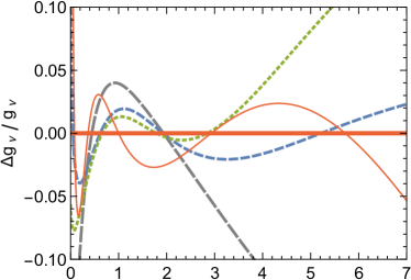
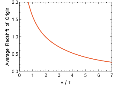
Figure 22: Spectral properties of the DSNB. Top: Maxwell-Boltzmann source spectrum with temperature $T$ (black) and corresponding DSNB spectrum (orange) for our fiducial redshift distribution of Yüksel et al. (2008). The dashed line is the fit function of Eq. (41); the fractional deviation is the red (thin solid) line the next panel. Middle: Fractional difference of the Mathews et al. (2014) case (gray, long dashed), the Robertson et al. (2015) case (blue, short dashed), and the Madau and Dickinson (2014) case (green, dotted) to the fiducial spectrum (red, thick solid). Bottom: Average of the source redshift for the fiducial case.

Overall the DSNB spectrum is fairly insensitive to the exact redshift distribution $f_{\rm cc}(z)$. In keeping with previous studies we use the distribution provided by Yüksel et al. (2008) as a fiducial case that was shown as a red line in the figures of this section.

In the bottom panel of Fig. 22 we show the average redshift contributing to the DSNB spectrum (only for our fiducial case) at a given energy. Even at the lower end of the detection interval, $\langle z\rangle$ is less than 1, and significantly smaller at higher energies. Therefore, the main contribution comes from relatively low redshifts.

The DSNB derived from a Maxwell-Boltzmann source spectrum is strongly anti-pinched (average energy for our fiducial case $\langle E\rangle=1.41\,T$ and pinching parameter 0.84) and not well represented by a Gamma distribution of the form of Eq. (33). However, one finds that the decreasing part of the spectrum is very close to an exponential $e^{-E/T}$ and a good overall fit to the fiducial case is

$$g_{\nu}(E/T)=1.15\,{\rm arctan}\bigl{[}3\,(E/T)^{3/2}\bigr{]}\,e^{-1.03\,E/T}.$$ (41)

The deviation of this fit from our fiducial spectrum is shown in the middle panel of Fig. 22 as a thin red line. The deviation is smaller than the spread of different cases of star-formation histories.

The main uncertainty of the DSNB prediction is the total number of core-collapse events shown in Eq. (40). Moreover, these predictions involve an overall uncertainty in converting the star-formation rate into a core-collapse rate (the factor $k_{\rm cc}$). A mismatch of about a factor of 2 between direct SN observations and the core-collapse rate estimated from star formation was found, the so-called SN-rate problem Horiuchi et al. (2011). The most likely explanation is dust extinction, especially at higher redshift, or a relatively large fraction of dim SNe, and in particular of non-exploding, BH forming cases Horiuchi et al. (2011, 2014); Adams et al. (2013); Kochanek (2014).

IX.4 Average emission spectrum

The sparse data of SN 1987A are not detailed enough to give a good estimate of the neutrino spectrum and also need not be representative of the average case. Therefore, DSNB predictions depend on numerical SN models. To get a first impression we assume that the time-integrated spectrum is of Maxwell-Boltzmann type. With Eq. (37) the DSNB flux for a given species $\nu$ is

$$\frac{d\Phi_{\nu}}{dE} = 4.45~{}{\rm cm}^{-2}~{}{\rm s}^{-1}~{}{\rm MeV}^{-1}~{}\frac{n_{\rm cc}}{10^{7}~{}{\rm Mpc}^{-3}}$$ (42)

$$\times \frac{6\,E^{\rm tot}_{\nu}}{2\times 10^{53}~{}{\rm erg}}\,\left(\frac{4~{}{\rm MeV}}{T}\right)^{2}\,g_{\nu}(E/T)\,,$$

where $E^{\rm tot}_{\nu}$ is the total emitted energy in the considered species $\nu$, and $g_{\nu}(E/T)$ is the normalised spectrum of Eq. (41) that includes our fiducial redshift distribution. We show this spectrum for $T=3.5$, 4, 4.5 and 6 MeV in Fig. 23, where values around 4 MeV would be typical for a core-collapse SN, whereas 6 MeV could represent a BH forming event with larger spectral energies.

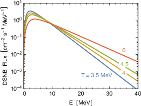
Figure 23: DSNB flux in one species according to Eq. (42). The emission spectrum is taken to be Maxwell-Boltzmann with the indicated temperatures.

Table 4: Characteristics of the time-integrated neutrino emission of the core-collapse models used to synthesize our illustrative DSNB example; for details see Møller et al. (2018). For each species $\nu$ we give the total number of emitted particles $N_{\nu}$, the emitted energy $E_{\nu}^{\rm tot}$, the average energy $E_{\rm av}$, the pinching parameter $\alpha$, and $E_{\rm av}^{\rm DSNB}$ after convolution with our fiducial redshift distribution. The remaining parameters determine the fit function of Eq. (43) for the normalised DSNB spectrum.

		$N_{\nu}$	$E_{\nu}^{\rm tot}$	$E_{\rm av}$	$\alpha$	$E_{\rm av}^{\rm DSNB}$	$a$	$b$	$q$	$p$	$T$
		$10^{57}$	$10^{52}~{}{\rm erg}$	MeV		MeV					MeV
$9.6\,M_{\odot}$ (SN)	$\nu_{e}$	2.01	3.17	9.8	2.81	4.59	1.347	1.837	1.837	0.990	2.793
	$\overline{\nu}_{e}$	1.47	2.93	12.4	2.51	5.83	1.313	1.770	1.703	0.969	3.483
	$\nu_{x}$	1.61	3.09	12.0	2.10	5.62	1.173	2.350	1.672	0.953	3.432
	$\overline{\nu}_{x}$	1.61	3.27	12.7	1.96	5.95	1.145	2.401	1.620	0.944	3.617
$27\,M_{\odot}$ (SN)	$\nu_{e}$	3.33	5.87	11.0	2.17	5.16	1.575	0.489	1.775	0.794	1.824
	$\overline{\nu}_{e}$	2.61	5.72	13.7	2.25	6.41	1.260	1.791	1.667	0.942	3.700
	$\nu_{x}$	2.56	5.21	12.7	1.88	5.95	1.153	2.106	1.615	0.916	3.400
	$\overline{\nu}_{x}$	2.56	5.53	13.5	1.76	6.32	1.111	2.337	1.569	0.916	3.690
$40\,M_{\odot}$ (BH)	$\nu_{e}$	3.62	9.25	16.0	1.66	7.47	1.065	2.340	1.809	0.866	3.904
	$\overline{\nu}_{e}$	2.88	8.61	18.7	1.99	8.75	1.089	3.199	1.801	0.951	5.486
	$\nu_{x}$, $\overline{\nu}_{x}$	1.72	4.83	17.5	1.46	8.21	1.227	1.090	1.314	0.822	3.707
Mix 1	$\langle\nu\rangle$	2.14	4.14	12.1	1.74	5.66	1.471	0.356	1.755	0.724	1.592
(59,32,9)	$\langle\overline{\nu}\rangle$	1.94	4.20	13.5	1.80	6.34	1.308	0.940	1.614	0.822	2.687
Mix 2	$\langle\nu\rangle$	2.09	4.25	12.7	1.52	5.95	1.362	0.318	1.768	0.690	1.486
(59,20,21)	$\langle\overline{\nu}\rangle$	1.88	4.26	14.2	1.64	6.63	1.301	0.734	1.617	0.777	2.439

        

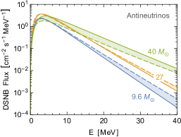
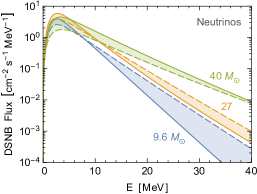
Figure 24: DSNB flux for the 9.6, 27 and $40\,M_{\odot}$ core-collapse models described in the text, where the actual flux would be a superposition of these reference cases. For each neutrino species, the flux is given by Eq. (44) with the parameters of Table 4. Solid lines are for $\nu_{e}$ or $\overline{\nu}_{e}$, dashed lines for $\nu_{x}$ or $\overline{\nu}_{x}$, so the flux for each mass eigenstate is a superposition of solid and dashed spectra, i.e., in the shaded bands, depending on flavor evolution upon leaving the source.

        

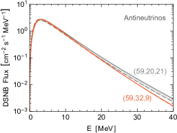
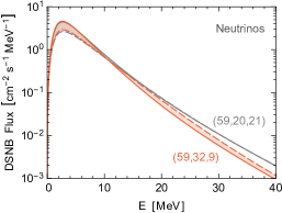
Figure 25: DSNB flux for the two indicated mixes of the 9.6, 27 and $40\,M_{\odot}$ source models.

We conclude that around the detection threshold of 10 MeV, the flux predictions are very similar and depend primarily on the overall normalization, i.e., the cosmic core-collapse rate and the average energy release. For larger $E$, the spectra scale essentially as $e^{-E/T}$ and thus depend strongly on the effective emission temperature. Therefore, the flux at the upper end of the detection window ($\sim 20$ MeV) is particularly sensitive to the fraction of BH forming events Nakazato et al. (2008); Lunardini (2009); Priya and Lunardini (2017); Møller et al. (2018); Schilbach et al. (2019).

More recent and sophisticated predictions synthesize the average emission spectrum from a suite of numerical SN models Nakazato et al. (2015); Horiuchi et al. (2018); Møller et al. (2018). Note that the high-energy tail of the DSNB spectrum is higher in these papers than what was adopted in the Super-Kamiokande analysis Bays et al. (2012) that was based on simplified modeling of the SN population and relied on older and more approximate SN models. For illustration, we here follow Møller et al. (2018) and consider three components, a $9.6\,M_{\odot}$ progenitor model, representing the range 8–$15\,M_{\odot}$ including electron-capture SNe, a $27\,M_{\odot}$ model, representing the higher-mass exploding cases, and a $40\,M_{\odot}$ non-exploding case called “slow BH formation” in Møller et al. (2018). Using a Salpeter initial mass function, the 8–$15\,M_{\odot}$ range encompasses 59% of all collapsing stars. The minimal prediction further assumes that the 15–$40\,M_{\odot}$ progenitors (32%) explode, and all progenitors with larger masses (9%) follow the slow-BH case. The fiducial case of Møller et al. (2018) assumes a larger fraction of 21% of BH formation, whereas an extreme case would be with 41% such cases, leaving only the 8–$15\,M_{\odot}$ range to explode.

We show the main characteristics of these spectral components in Table 4. The exploding models use four-species neutrino transport and thus provide separate emission spectra for $\nu_{e}$, $\overline{\nu}_{e}$, $\nu_{x}$ and $\overline{\nu}_{x}$. For each model and each species we show the total number of emitted particles $N_{\nu}$, the emitted energy $E^{\rm tot}_{\nu}$, and the average neutrino energy $E_{\rm av}$ and pinching parameter $\alpha$ of the time-integrated spectrum. The overall emitted energy is $E_{\rm tot}=E^{\rm tot}_{\nu_{e}}+E^{\rm tot}_{\overline{\nu}_{e}}+2E^{\rm tot}_{\nu_{x}}+2E^{\rm tot}_{\overline{\nu}_{x}}$. We convolve these emission spectra with our fiducial redshift distribution, which does not change $N_{\nu}$ but only the spectral shape. Inspired by Eq. (41), we approximate the spectra by fit functions of the form

$$g_{\nu}(E)=\frac{a}{T}\,{\rm arctan}\left[b\left(\frac{E}{T}\right)^{q}\right]\,\exp\left[-\left(\frac{E}{T}\right)^{p}\right]\,,$$ (43)

where the global factor $a$ is constrained by normalization $\int_{0}^{\infty}dE\,g_{\nu}(E)=1$. In the measurement region, $E\gtrsim 10~{}{\rm MeV}$, the spectrum scales as $\exp[-(E/T)^{p}]$ with $p\sim 1$. The fit parameter $T$ sets the energy scale and is one way of defining an effective temperature for the non-thermal emission spectrum. For a given species $\nu$, the DSNB flux is

$$\frac{d\Phi_{\nu}}{dE}=\frac{10.3}{{\rm cm}^{2}~{}{\rm s}~{}{\rm MeV}}\,\frac{n_{\rm cc}}{10^{7}~{}{\rm Mpc}^{-3}}\,\frac{N_{\nu}}{10^{57}}\,g_{\nu}(E)\,,$$ (44)

where the parameter $T$ is assumed to be in units of MeV. These fits represent the numerical spectra to better than a few percent, especially in the detection region. The fractional deviation always looks similar to the dashed red line in the middle panel of Fig. 22.

We show the DSNB fluxes for each species in Fig. 24 for each core-collapse model as if the entire DSNB was caused by only one of them. The higher-mass models, with a longer period of accretion, have hotter spectra, especially the BH forming case. For the exploding cases, the $x$ spectra provide larger fluxes at high energies than the $e$-flavored ones, whereas for the BH case, it is opposite because the long accretion period produces larger fluxes of $\nu_{e}$ and $\overline{\nu}_{e}$ than of the other species.

In Fig. 25 we show DSNB fluxes based on the minimal case of Møller et al. (2018) with a mixture of 59, 32 and 9% of the 9.6, 27 and $40\,M_{\odot}$ models (red) and their fiducial case with 59, 20 and 21% (gray). It is intriguing that the mixed cases show a much smaller spread between the flavor-dependent spectra (solid vs. dashed lines). This effect partly owes to the inverted flavor dependence between the exploding and non-exploding models. Moreover, near the detection threshold of around 10 MeV, the exact mix leaves the DSNB prediction nearly unchanged.

IX.5 Flavor Conversion

Neutrinos are produced with flavor-dependent fluxes and spectra so that flavor conversion on the way from the decoupling region modifies the escaping flavor composition, or rather, the final mix of mass eigenstates. Moreover, in which way this effect is relevant depends on the detection method. As argued in Sec. VIII.6, SN neutrino flavor conversion is not yet fully understood, so by the current state of the art, there is no reliable prediction. On the other hand, flavor conversion would be a small effect on the overall DSNB prediction as seen in Fig. 25, where the difference between the dashed and solid lines is quite small, especially near the detection threshold of 10 MeV where most events would be measured.

Therefore, as a baseline prediction we use fluxes that are flavor averages of the form $\Phi_{\langle\nu\rangle}=(\Phi_{\nu_{e}}+2\Phi_{\nu_{x}})/3$. We show the spectral characteristics for our two illustrative mixtures in Table 4. For our minimal Mix 1, we find a total DSNB flux, number density, and energy density at Earth of neutrinos plus antineutrinos of all flavors that was shown in Eq. (34). Concerning normalization, the main uncertainty is the overall core-collapse rate. Concerning the spectral shape, the main uncertainty is the fraction of BH-forming cases.

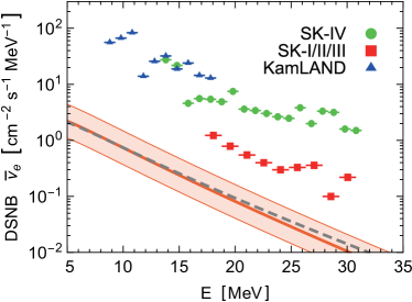
Figure 26: Experimental limits on the $\overline{\nu}_{e}$ component of the DSNB by Super-Kamiokande (SK) I/II/III Bays et al. (2012), SK IV Zhang et al. (2015), and KamLAND Gando et al. (2012). [Plot of limits adapted from Nakazato et al. (2015) with permission.] The fiducial predicted flux is our Mix 1 (red solid) with an adopted normalization uncertainty of a factor of 2 in either direction (shaded band). We also show Mix 2 (gray dashed) that includes a larger fraction of BH-forming cases.

IX.6 Detection perspectives

The DSNB has not yet been detected, but the experimental limits shown in Fig. 26 have been obtained by the Super-Kamiokande (SK) I/II/III water Cherenkov detector Bays et al. (2012), SK IV with neutron tagging Zhang et al. (2015), and the KamLAND liquid scintillator detector Gando et al. (2012). All of these limits are based on the inverse-beta decay reaction $\overline{\nu}_{e}+p\to n+e^{+}$. These limits do not yet reach predictions, but keeping in mind that the cosmic core-collapse rate and its BH forming component could be larger than assumed here means that any significant experimental improvement can lead to a detection.

DSNB detection is not only a question of event rate, but of identification and rejection of several backgrounds that can mimic DSNB events. A first detection should become possible over the next decade with the upcoming Gd-enhanced Super-Kamiokande water Cherenkov detector Beacom and Vagins (2004); Labarga (2018) and later with a possible Gd-enhanced version of the upcoming Hyper-Kamiokande Abe et al. (2018). Another promising contender is the upcoming JUNO 20 kt scintillator detector An et al. (2016). A complementary detection channel, using the $\nu_{e}$ flux, may be offered by the upcoming liquid argon detector DUNE at the LBNF facility in the US Cocco et al. (2004); Acciarri et al. (2016). A detailed forecast of these opportunities is beyond the scope of our discussion.

X Atmospheric Neutrinos

Atmospheric neutrinos are produced by cosmic rays interacting with the Earth or Sun atmosphere Seckel et al. (1991); Ingelman and Thunman (1996); Gaisser et al. (2016); Ng et al. (2017); Edsjö et al. (2017); Argüelles et al. (2017); Ng et al. (2017). Historically, they were the first “natural neutrinos” to be detected Achar et al. (1965); Reines et al. (1965) and later played a fundamental role in establishing flavor oscillations by the Super-Kamiokande water Cherenkov detector Fukuda et al. (1998). Nowadays, atmospheric neutrinos are employed to measure the neutrino mass and mixing parameters with high precision, while on the other hand they are a background to the detection of astrophysical neutrinos.

X.1 Cosmic rays

Charged particles like electrons, protons and heavier nuclei are accelerated within cosmic reservoirs or on their way to Earth in the presence of astrophysical shocks and magnetic turbulence. These particles constitute the cosmic-ray flux. It further interacts with the Earth atmosphere, producing a secondary particle flux that includes neutrinos. The origin of cosmic rays as well as their composition (the fraction of heavy nuclei and protons) remains subject of vivid debate. The correspondent neutrino flux depends on the cosmic-ray composition, the scattering cross section with the atmosphere as well as radiative losses, and the branching ratios of the by-products.

Comparing the cosmic-ray composition with the chemical composition of the solar system reveals interesting differences Gaisser et al. (2016). One is that the relative contribution of heavy nuclei with respect to hydrogen is larger in cosmic rays Dartois et al. (2015); Wang et al. (2002); de Nolfo et al. (2006); George et al. (2009); Lodders (2003). This could be due to the relative greater ionization energy of hydrogen compared to heavy elements; in fact only ionized or charged particles can be accelerated. An additional, straightforward reason could be a difference in the source composition itself Cassé et al. (1975). Finally, for volatile elements, it is possible that this could be due to a mass-to-charge dependence of the acceleration efficiency, with heavier ions being more favorably accelerated Meyer et al. (1997). Another striking difference is that two groups of elements (Li, Be and B is one; Sc, Ti, V, Cr, and Mn the other) are more abundant in cosmic rays. This is because they are produced in spallation processes (scattering of cosmic rays in the interstellar medium) instead of stellar nucleosynthesis Tanabashi et al. (2018).

Turning to the energy distribution, above 10 GeV a good approximation to the differential spectrum per nucleon is given by an inverse power law of the form

$$\frac{dN_{N}}{dE}\propto E^{-(\gamma+1)}\ ,$$ (45)

where $\gamma\approx 1.7$ up to around $3\times 10^{6}$ GeV, e.g., $\gamma_{\rm{proton}}=1.71\pm 0.05$ Gaisser et al. (2016), and $\gamma\approx 2.0$ at larger energies. This spectral break is known as the knee of the cosmic-ray flux. A second break, known as second knee, is near $10^{8}$ GeV. Near $3\times 10^{9}$ GeV there is another break known as the ankle. Including the normalization given in Tanabashi et al. (2018), the spectrum between several GeV and 100 TeV is

$$\frac{dN_{N}}{dE}=\frac{1.8\times 10^{4}}{(\mbox{GeV/nucleon})~{}\mbox{m}^{2}~{}\mbox{s}~{}\mbox{sr}}\left(\frac{E}{\mbox{GeV/nucleon}}\right)^{-(\gamma+1)}\!\!.$$ (46)

Below $10$ GeV, all cosmic-ray spectra show “solar modulation” Gleeson and Axford (1968); Strauss et al. (2012); Maccione (2013); Cholis et al. (2016), a time variation caused by the solar wind, a low-energy plasma of electrons and protons ejected by the Sun with its 11 year cycle. The shield-like effect of the solar activity translates to an anti-correlation between the latter and cosmic-ray spectra. Moreover, low-energy particles entering the atmosphere also suffer geomagnetic effects. Therefore, low-energy secondary particle fluxes, including neutrinos, depend on both location and time.

X.2 Conventional neutrinos

Cosmic rays entering the atmosphere scatter and produce secondary particles, especially charged or neutral pions and kaons, which in turn decay and produce the “conventional neutrinos” Stanev (2004) as a main contribution at low energies. The detailed decay chains are

$$\pi^{\pm}\to\, \mu^{\pm}+\nu_{\mu}(\overline{\nu}_{\mu})$$

$$\downarrow$$

$$e^{\pm}+\nu_{e}(\overline{\nu}_{e})+\overline{\nu}_{\mu}(\nu_{\mu})\ ,$$ (47)

$$K^{\pm}\rightarrow\mu^{\pm}+\nu_{\mu}(\overline{\nu}_{\mu})\ .$$ (48)

Three-body decays of kaons also occur, for example

$$K^{\pm}\rightarrow\pi^{0}+e^{\pm}+\nu_{e}(\overline{\nu}_{e})\ .$$ (49)

Some of the kaons decay purely into pions, for example in processes such as

$$K^{\pm}\rightarrow\pi^{\pm}+\pi^{0}\ ,$$ (50)

which in turn produce neutrinos. On the other hand, cosmic rays also produce $\pi^{0}$ that decay to photons

$$\pi^{0}\rightarrow\gamma+\gamma\ ,$$ (51)

establishing a connection between high-energy astrophysical photons and neutrinos (see Sec. XI).

Up to 1 GeV, all muons decay before reaching the ground, implying a neutrino $\mu/e$ flavor ratio of

$$\frac{\nu_{\mu}+\overline{\nu}_{\mu}}{\nu_{e}+\overline{\nu}_{e}}\simeq 2\ .$$ (52)

At somewhat higher energies, $\mu$ decay becomes negligible and $\pi$ and $K$ decays dominate. The resultant $\nu_{\mu}$ plus $\overline{\nu}_{\mu}$ flux is given by the fit Stanev (2004); Gaisser and Honda (2002); Gaisser (2019)

$$\frac{dN_{\nu}}{dE_{\nu}}\simeq{} 0.0096\,\frac{1}{\rm cm^{2}\,s\,sr\,GeV}\left(\frac{E_{\nu}}{\rm GeV}\right)^{-2.7}$$

$${}\times\left(\frac{1}{1+\frac{3.7E_{\nu}\cos\theta}{\epsilon_{\pi}}}+\frac{0.38}{1+\frac{1.7E_{\nu}\cos\theta}{\epsilon_{K}}}\right)\ ,$$ (53)

where $\epsilon$ is the energy scale for the most probable process in propagation (decay vs. interaction); for pions $\epsilon_{\pi}\simeq 115$ GeV and for kaons $\epsilon_{K}\simeq 850$ GeV. Moreover, $\theta$ is the zenith angle of observation.

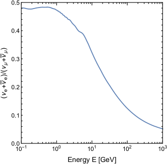
Figure 27: Atmospheric neutrino $e/\mu$ flavor ratio, corresponding to the source fluxes (no oscillations) shown in Fig. 28.

Asymptotically at high energies the $\pi:K$ neutrino production is $1:3$. The resultant flavor is mainly muonic, while the electronic one becomes negligible as shown in Fig. 27. This feature can be understood observing that, at high enough energies, the muon neutrino flux scales as $E_{\nu}^{-3.7}$ while electron neutrinos originating from muons scale as $E_{\nu}^{-4.7}$, where the extra power of $E_{\nu}^{-1}$ comes from the muon Lorentz factor that reduces its decay probability, making scattering more likely. At some energy, of course, the $\nu_{e}$ and $\overline{\nu}_{e}$ produced directly by kaon decays take over and then their flux also scales as $E_{\nu}^{-3.7}$, but with a much smaller flux than the muon flavor.

In first approximation, atmospheric neutrinos seen by a detector at or below the ground are isotropic. The atmospheric source mass intersected by a differential solid angle $d\Omega$ scales with $r^{2}$ which cancels exactly the geometric $1/r^{2}$ flux dilution, where $r$ is the distance between detector and atmosphere in the chosen direction.

There are important corrections to this simple picture. In fact in the few-GeV range, that was crucial for establishing flavor oscillations, the flux is essentially up-down symmetric, but it is enhanced in the horizontal direction because there is a longer decay path before muons reach the ground Gaisser and Honda (2002); Honda et al. (2004); Stanev (2004). A similar effect pertains at high energies for kaon decays.

At energies beyond a few TeV, the Earth is no longer completely transparent to neutrinos so that the flux from below is diminished Nicolaidis (1988); Nicolaidis et al. (1991); Gonzalez-Garcia et al. (2008); Donini et al. (2019). For energies up to about 1 PeV, neutrinos of any flavor are more efficiently absorbed than antineutrinos because they scatter on nuclei, while the scattering on electrons is negligible. Nuclei in the Earth matter are heavy and contain more neutrons (quark content $udd$) than protons (quark content $uud$). Taking into account that neutrinos (respectively antineutrinos) can exchange a $W$ boson with $d$ (respectively $u$), the reaction $\nu+A\rightarrow l+B$ becomes more likely than $\overline{\nu}+A\rightarrow l+B$. With increasing energy, valence quarks become negligible relative to sea quarks, so the cross sections of $\nu$ and $\overline{\nu}$ become asymptotically equal. The only exception is provided by the Glashow resonance Glashow (1960)

$$\overline{\nu}_{e}+e^{-}\rightarrow W^{-}\rightarrow X$$ (54)

at $E_{\nu}\simeq m_{W}^{2}/2m_{e}\simeq 6$ PeV, so there is a region in which $\overline{\nu}_{e}$ are more likely to be absorbed than $\nu_{e}$.

X.3 Prompt neutrinos

Atmospheric neutrinos produced by charmed mesons are called prompt neutrinos Volkova (1980); Gondolo et al. (1996); Pasquali and Reno (1999); Enberg et al. (2008); Gaisser (2019). They consist of equal amounts $e$ and $\mu$ flavor and a very small $\tau$ component. The prompt flux contribution was expected to be large in the TeV to PeV range ($\epsilon_{\rm charm}\simeq$ PeV), where the only other contribution comes from kaon decay. The latter is distinguishable thanks to its angular distribution which is enhanced in the horizontal direction because of the larger kaon decay path. Prompt neutrinos, instead, are isotropic up to high energies because of the short charmed-meson lifetime of $10^{-12}$–$10^{-13}$ s. Moreover, the prompt flux is harder so that it will dominate beyond a certain energy. Semi-analytical expressions for the prompt flux can be found in Volkova and Zatsepin (1999). The uncertainty in the estimates of this flux is quite large Garzelli et al. (2017); while conventional atmospheric neutrino predictions are affected by a $\sim 10\%$ uncertainty Honda et al. (2007), the prompt flux has large uncertainties due to poor knowledge of the charm meson production processes Garzelli et al. (2015).

Concerning recent developments, IceCube has not found a significant prompt component Aartsen et al. (2015b, 2016c). Moreover, recent calculations accounting for the latest measurements of the hadronic cross sections predict a prompt neutrino flux that is generally lower than its previous benchmark estimation Bhattacharya et al. (2016).

X.4 Predictions and observations

To predict the atmospheric neutrino flux one needs to solve a set of transport equations, which are coupled integro-differential equations. While semi-analytical approximations exist, numerical solutions are more reliable. To reproduce the theoretically expected flux in Fig. 28 (dashed lines), we use the tables publicly available on Mitsuhito Honda’s homepage Honda et al. (2015). For the very low energy ($\lesssim 100\,\rm MeV$) flux, included in Fig. 1, we use FLUKA results Battistoni et al. (2005). We choose Kamioka as a site because the geographic dependence is more important for low-energy neutrinos which are measured mostly by Super-Kamiokande. Because we are not aiming for a high-precision fit, we consider the flux under the mountain in Kamioka and take the Sun at average magnetic activity. As explained earlier, the $\mu/e$ flavor ratio begins approximately at 2 at low energies and then increases. Concerning uncertainties, the authors of Fedynitch et al. (2012) have quantified the systematic influence caused by the choice of primary cosmic-ray flux models and the interaction model. The average errors on the $\nu_{\mu}$ and $\nu_{e}$ fluxes at high energies were found to be ${}^{+32\%}_{-22\%}$ and ${}^{+25\%}_{-19\%}$ respectively.

Neutrinos produced in the atmosphere can change flavor before reaching the detector. For the given mixing parameters (Appendix B) and for GeV energies, $\nu_{e}$ and $\overline{\nu}_{e}$ remain essentially unaffected, because the mean weak potential describing the Earth matter effect is large compared with $\delta m^{2}/2E$ and because they have only a small admixture of the third mass eigenstate. The main effect derives from two-flavor oscillations in the $\nu_{\mu}$-$\nu_{\tau}$ sector, driven by the “atmospheric mass difference” $\Delta m^{2}\sim(50~{}{\rm meV})^{2}$ with an oscillation length $L_{\rm osc}=4\pi E/\Delta m^{2}\sim 990~{}{\rm km}~{}E/{\rm GeV}$. Therefore, neutrinos from above show the primary flavor content, whereas those from below, after traveling thousands of kilometers, show significant $\nu_{\mu}$ disappearance. This up-down asymmetry was the smoking-gun signature detected by Super-Kamiokande Fukuda et al. (1998) and honored with the 2015 Physics Nobel Prize for Takaaki Kajita.

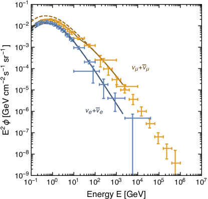
Figure 28: Atmospheric neutrino flux per solid angle, averaged over directions, as a function of energy for $\nu_{\mu}+\overline{\nu}_{\mu}$ (upper curve, orange) and $\nu_{e}+\overline{\nu}_{e}$ (lower curve, blue). The data points at low and medium energies represent the Super-Kamiokande observations Richard et al. (2016) and of IceCube at high energies Aartsen et al. (2015c, d). The dashed lines are theoretical predictions at the Kamioka site for average solar activity Honda et al. (2015); the solid lines are the expected fluxes including flavor oscillations. The $\nu_{\tau}+\overline{\nu}_{\tau}$ flux appearing in this case is not shown, corresponding to the difference between the orange dashed and solid lines. We thank F. Capozzi for providing the tables used to include oscillations.

The solid lines in Fig. 28 show the predicted angle-averaged fluxes when flavor oscillations are included. Without aiming for a precision comparison in our plot, they agree well with the measured fluxes which are taken from Super-Kamiokande at low and medium energies ($10^{-1}$–$10^{3}$ GeV) Richard et al. (2016) and from IceCube at high energies ($10^{2}$–$10^{6}$ GeV) Aartsen et al. (2015c, d). While the primary $\nu_{\tau}$ flux of prompt neutrinos is very small, there is a large $\nu_{\tau}$ component from flavor conversion that we do not show and that is difficult to measure because of the short lifetime of the $\tau$ lepton produced in charged-current interactions. It was only recently that first evidence for atmospheric $\nu_{\tau}$ appearance was reported by IceCube DeepCore Aartsen et al. (2019).

X.5 Experimental facilities

The main experimental facilities sensitive to atmospheric neutrinos have been IceCube Aartsen et al. (2015c, d), Super-Kamiokande Richard et al. (2016), SNO Aharmim et al. (2010), and MINOS Adamson et al. (2011). SNO, although mainly built to detect solar neutrinos, also detected high-energy atmospheric neutrinos. SNO was located 2 km underground, and therefore near-horizontal downward-going muons with typical energies of 100 GeV originated as a result of the atmospheric neutrino interactions. Given the measured atmospheric $\Delta m^{2}$, the effect of flavor conversion is tiny for the near-horizontal downward-going muons. Hence, these muon data were used to calibrate the estimated atmospheric neutrino flux. SNO is currently being replaced with its successor SNO+ Lozza (2019), which however does not have atmospheric neutrinos as a main goal for the next future. MINOS was a long-baseline neutrino oscillation experiment and has been the first magnetized tracking detector for atmospheric neutrinos.

IceCube measures atmospheric neutrinos as a background for very high-energy astrophysical neutrinos in the range 100 GeV–400 TeV. Neutrinos with energies up to 1 GeV will have the final-state particle “fully contained” in the detector. Muon neutrinos with higher energies may result in a muon leaving the detector, the so-called “partially contained” events. To measure the atmospheric flux accurately, it is important to pinpoint the vertex position of the interaction and classify the neutrino event accordingly. IceCube DeepCore Abbasi et al. (2012) is an infill of 8 strings added to the IceCube array and is dedicated to the detection of neutrinos with energy below 100 GeV. Similarly to IceCube, the deep-sea Cherenkov detectors, ANTARES and its successor Km3NeT Van Elewyck (2019), allow us to exploit atmospheric neutrinos to study flavor oscillation physics.

The largest statistics of atmospheric neutrinos for neutrino oscillation studies is dominated by the Super-Kamiokande data. Hyper-Kamiokande Abe et al. (2018) will provide an even larger amount of data.

Among the detectors specifically dedicated to the observation of atmospheric neutrinos, there is the project of the India-based Neutrino Observatory (INO) Indumathi (2015). It will be located in a 1.2 km deep cave near Theni in India. INO promises to provide a precise measurement of neutrino mixing parameters.

X.6 Solar atmospheric neutrinos

An additional contribution to the GUNS comes from the Sun in the form of “solar atmospheric neutrinos” that are produced by cosmic-ray interactions in the solar atmosphere Ingelman and Thunman (1996); Ng et al. (2017); Edsjö et al. (2017); Argüelles et al. (2017). While the production processes are analogous to those in the Earth atmosphere, the Sun atmosphere is thinner so that pions and kaons can travel much larger distances without collisions. This results in a neutrino flux that is both larger and harder at high energies as shown in Fig. 29. The detection of low-energy ($\lesssim 1\rm\,TeV$) solar atmospheric neutrinos, while not possible with on-going experiments, would be very useful to probe the magnetic field of the solar atmosphere Ng et al. (2017).

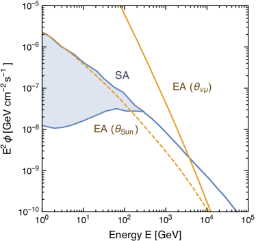
Figure 29: The $\nu_{\mu}+\overline{\nu}_{\mu}$ solar atmospheric neutrino (SA) flux (blue) compared to the Earth (EA) one (orange), the latter integrated over the solar angular cone (dashed) and over the muon-neutrino angular cone (solid), see Ng et al. (2017) and references therein. The SA uncertainty at low energies (blue shaded region) is due to the modelling of the magnetic fields at the solar surface and those carried by the solar wind. We thank Kenny C. Y. Ng for providing the data for this figure.

The fluxes shown in Fig. 29 correspond to Fig. 1 of Ng et al. (2017), where the authors assumed the solar magnetic field of Seckel et al. (1991) for the flux up to 300 GeV and the model of Ingelman and Thunman (1996) at larger energies. What is shown is the primary $\nu_{\mu}+\overline{\nu}_{\mu}$ flux that will be diminished by flavor oscillations before reaching Earth.

To compare the solar flux with the diffuse background of Earth atmospheric neutrinos, the latter must be integrated over a suitable solid angle. A naive estimate is the solar angular cone $\theta_{\rm Sun}\simeq 0.17^{\circ}$ (dashed orange line in Fig. 29). However, muons coming from different directions can decay producing neutrinos along a direction lying in the solar angular cone, so the flux must be integrated over the energy-dependent muon-neutrino separation angle $\theta_{\nu\mu}\simeq 1^{\circ}\sqrt{\rm 1\,TeV/E_{\nu}}$ Ng et al. (2017) (solid orange line in Fig. 29 marked EA).

The detection of high-energy ($\gtrsim 1\,\rm TeV$) solar atmospheric neutrinos is conceivable in ten years of data taking by IceCube and KM3NeT Ng et al. (2017); In and Jeong (2018), and would mark an important milestone for neutrino astronomy, as well as being an important calibration source for future neutrino telescopes in different hemispheres.

XI Extra-terrestrial high energy neutrinos

The era of high-energy neutrino astronomy was born with the detection of neutrinos of astrophysical origin by the IceCube Neutrino Observatory Aartsen et al. (2013b, a, 2016c). These events have energies between few TeV to few PeV. Their arrival directions do not exhibit anisotropies, suggesting that only up to $\sim 1\%$ of the observed flux may come from our Galaxy Denton et al. (2017); Albert et al. (2018); Ahlers and Murase (2014). More neutrinos are instead expected from sources distributed on cosmological scales, such as dim or choked astrophysical jets, star-forming galaxies (SFGs), gamma-ray bursts (GRBs), active galactic nuclei (AGNs), and galaxy clusters. For recent dedicated reviews see for example Ahlers and Halzen (2018), Ahlers et al. (2018), Mészáros (2017), Waxman (2017), and Murase (2017).

XI.1 Production mechanisms and detection prospects

Neutrinos in the energy range of interest are produced by cosmic-ray interactions in the source, its surroundings, or during cosmic-ray propagation en route to Earth. The reactions involve proton-proton (“$pp$”) or proton-photon (“$p\gamma$”) interactions, leading to the following production channels for neutrinos and gamma rays: $\pi^{0}\rightarrow\gamma+\gamma$, $\pi^{\pm}\rightarrow\mu^{\pm}+\nu_{\mu}(\overline{\nu}_{\mu})$ and $\mu^{\pm}\rightarrow e^{\pm}+\overline{\nu}_{\mu}(\nu_{\mu})+\nu_{e}(\overline{\nu}_{e})$ in analogy to atmospheric neutrino production (Sec. X.2).

Before absorption and reprocessing of very high-energy $\gamma$ rays, the relative fluxes of neutrinos and gammas is approximately regulated by the ratio of $\pi^{\pm}$ to $\pi^{0}$ production, whereas the $\nu$ flavor distribution would be $\nu_{e}:\nu_{\mu}:\nu_{\tau}\simeq 1:2:0$. After a long distance of propagation, the oscillation-averaged composition reaching the detector is expected to be $\nu_{e}:\nu_{\mu}:\nu_{\tau}\simeq 1:1:1$ Learned and Pakvasa (1995); Farzan and Smirnov (2008).

The diffuse neutrino intensity at Earth from extragalactic sources is given by the integral of the spectral distribution for each source, $F_{\nu_{\alpha}}$, convolved with the source distribution (a function of redshift $z$ and source luminosity $L$) over the co-moving volume $\rho(z,L)$

$$\phi(E_{\nu}) = \frac{1}{4\pi}\int_{0}^{\infty}\!dz\int_{L_{\rm min}}^{L_{\rm max}}dL_{\nu}\,\frac{1}{H(z)}\rho(z,L_{\nu})$$ (55)

$$\kern 60.00009pt{}\times\sum_{\alpha}F_{\nu_{\alpha}}\left[(1+z)E_{\nu}\right]\,,$$

with $H(z)$ being the Hubble factor at redshift $z$.

This equation can be approximately expressed in the form Waxman and Bahcall (1999)

$$\phi_{\nu}=\xi\,\frac{L_{\nu}n_{\rm s}R_{H}}{4\pi}\ ,$$ (56)

where $\xi$ accounts for the redshift evolution of sources ($\xi=2$ or 3 is usually assumed for sources following the star-formation rate), $n_{\rm s}$ is the source density, and $R_{H}=c/H_{0}\simeq 400$ Mpc is the Hubble radius. Comparing Eq. (56) with the diffuse flux observed by IceCube ($2.8\times 10^{-8}$ GeV$/$cm² s sr), we obtain Gaisser et al. (2016)

$$n_{\rm s}L_{\nu}=\frac{4\times 10^{43}}{\xi}\frac{\mathrm{erg}}{\mathrm{Mpc}^{3}~{}\mathrm{yr}}\sim 10^{43}\frac{\mathrm{erg}}{\mathrm{Mpc}^{3}~{}\mathrm{yr}}\ .$$ (57)

This relation provides the minimum power density necessary to produce the neutrino flux observed by IceCube. Hence any viable neutrino source needs to sit above the line defined by Eq. (57) in the luminosity-density plane in Fig. 30; such a plot was originally shown in various forms in Silvestri and Barwick (2010), Murase et al. (2012), and Kowalski (2015).

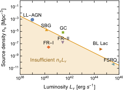
Figure 30: Source density vs. neutrino luminosity for potential sources of high-energy neutrinos. The markers are examples of benchmark astrophysical sources: low-luminosity active galactic nuclei (LL-AGN), starburst galaxies (SBG), galaxy clusters (GC), BL Lacertae objects (BL-Lac), Fanaroff-Riley galaxies of type I and II (FR-I and FR-II), flat-spectrum radio quasars (FSRQ). See Mertsch et al. (2017) and Ackermann et al. (2019) for details on the estimation of $(L_{\nu},n_{\rm s})$.

XI.2 Multi-messenger connections

Assuming that all particles populating the high-energy sky originate from the same source classes, the cosmic energy density of high-energy neutrinos should be connected to the one of $\gamma$-rays observed by the Fermi Telescope Fornasa and Sánchez-Conde (2015) and to the one of ultra-high-energy cosmic rays seen by the Auger Observatory Grenier et al. (2015), see e.g. Murase et al. (2013) and Ahlers and Halzen (2018) for more details.

The extragalactic $\gamma$-ray background observed by Fermi derives from point-like sources and an isotropic component. Intriguingly, the current IceCube data cannot be consistently interpreted by employing the same composition of sources. This is especially true for the 10–100 TeV neutrino energy spectrum that cannot be fitted by invoking a common origin for neutrinos and $\gamma$-rays Denton and Tamborra (2018c); Murase et al. (2016).

A direct correlation between TeV–PeV neutrinos and ultra-high-energy cosmic rays should also exist, but no clear evidence has been found yet Aartsen et al. (2016d); Moharana and Razzaque (2015). Cosmic rays could be trapped in the source because of strong magnetic fields and hence produce neutrinos through collisions with the gas. The efficiency of this process is related to the total energy stored in the source under the assumption that it is calorimetric.

Cosmic rays above $3\times 10^{18}$ eV are thought to be of extragalactic origin, while a mainly galactic origin is expected at smaller energies. The observation of extragalactic cosmic rays allows one to establish an upper bound on the fluence of neutrinos of astrophysical origin produced in cosmic reservoirs; this leads to the so-called Waxman and Bahcall bound Waxman and Bahcall (1999); Bahcall and Waxman (2001)

$$E_{\nu}\phi_{\nu}<2\times 10^{-8}\xi~{}\mathrm{GeV}/(\mathrm{cm}^{2}~{}\mathrm{s}~{}\mathrm{sr})\,,$$ (58)

where $\xi$ is the same as in Eq. (56). Equation (58) should be considered as an upper limit on neutrino emission from the sources of ultra-high-energy cosmic rays under the assumption that the spectrum scales as $E^{-2}$, as predicted by Fermi acceleration. Notably, the Waxman and Bahcall bound was derived under the assumption that sources are optically thin to photo-meson and proton-nucleon interactions such that protons are free to escape. If optically thick sources exist, this bound does not hold.

High-energy neutrinos are emitted by a plethora of astrophysical sources, however we will focus on SFGs, GRBs and AGNs. These are the most efficient neutrino emitters. In particular, for what concerns AGNs, we will focus on a sub-class, blazars, currently considered to constitute the bulk of the extra-galactic $\gamma$-ray diffuse emission Ackermann et al. (2016). Notably, a dozen of the IceCube neutrino events is likely to be connected to a blazar Aartsen et al. (2018b, a), but given their energy, those neutrino events do not contribute to the diffuse IceCube flux. The non-detection of point sources generating multiple neutrino events from astrophysical sources provides a lower limit on the local density of these sources and an upper limit on their effective neutrino luminosity Murase and Waxman (2016); Mertsch et al. (2017). Finally, we will discuss the predicted flux of cosmogenic neutrinos, produced by cosmic-ray interactions en route to Earth.

XI.3 Star-forming galaxies

SFGs are stationary sources compared with transient ones, such as GRBs and AGNs, that will be discussed later. SFGs are perfect examples of calorimetric sources Loeb and Waxman (2006); Waxman (2017). Presumably they produce high-energy neutrinos mostly through $pp$ interactions Loeb and Waxman (2006); Thompson et al. (2006); Lacki et al. (2011).

Beyond normal galaxies, such as our Milky Way, another class of SFGs consists of starburst galaxies. These are individually more luminous than SFGs as they undergo a phase of enhanced star-formation activity (up to 100 times higher than normal galaxies).

Our understanding of star formation has dramatically improved in the last decade. In particular, the Herschel Space Observatory Gruppioni et al. (2013) provided an unprecedented estimation of the infrared luminosity function of SFGs up to redshift 4 and made possible the distinction among different sub-classes. In fact, beyond normal and starburst galaxies, Herschel provided for the first time information on SFGs containing low-luminosity AGNs or AGNs obscured by dust (after correcting for the contribution of AGNs Gruppioni et al. (2013)). All these classes contribute to the star-formation activity.

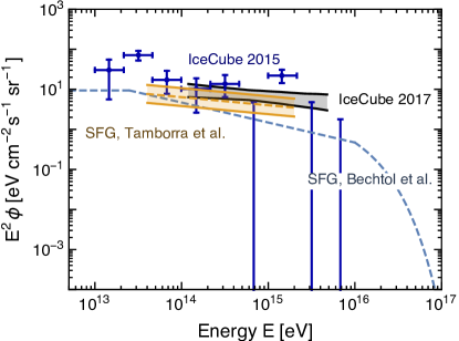
Figure 31: Diffuse neutrino flux per flavor $\nu_{\alpha}+\overline{\nu}_{\alpha}$ from SFGs. The dashed line reproduces the results of Bechtol et al. (2017), where an upper limit to the contribution from blazars was calculated by analyzing the $\gamma$-ray flux. The orange band (marked “SFG, Tamborra et al.”) reproduces the results of Tamborra et al. (2014a) based on the infrared data. Notice that the spectral shape is slightly different given the different injection spectral indexes adopted in the theoretical estimations. Also shown is the IceCube neutrino flux per flavor according to Aartsen et al. (2015a) (data points) and a more recent estimation including high-energy data only Aartsen et al. (2017c) (black band marked “IceCube 2017”).

Among all galaxies, about $38\%$ are normal, $7\%$ are of starburst type, and the remaining ones are SFGs containing AGNs. The abundance of each class varies as a function of redshift, with normal galaxies being more abundant at low redshifts ($z<1.5$). The $\gamma$-ray energy distribution of normal galaxies is observed to be softer ($F_{\gamma}\propto E_{\gamma}^{-2.7}$) on average than the one of starburst galaxies ($F_{\gamma}\propto E_{\gamma}^{-2.2}$–$E_{\gamma}^{-2.3}$ Ackermann et al. (2012); Bechtol et al. (2017). Finally, star-forming galaxies containing active galactic nuclei can have an energy spectral distribution resembling normal galaxies or starburst galaxies depending on redshift Tamborra et al. (2014a).

Neutrinos are thought to be produced in SFGs through $pp$ interactions under the assumption that $\mathcal{O}(100)$ PeV cosmic rays are produced and confined in these sources. This assumption might be optimistic given that the Galactic cosmic-ray spectrum breaks at $3$ PeV.

As a consequence of $pp$ interactions in the source, a direct connection between the estimated neutrino and $\gamma$-ray emission can be established Thompson et al. (2006); Lacki et al. (2011); Tamborra et al. (2014a); Senno et al. (2015); Sudoh et al. (2018). One can then estimate the neutrino emission following the modelling proposed in Tamborra et al. (2014a) using the infrared data from the Herschel Space Observatory Gruppioni et al. (2013). As the infrared luminosity function is connected to that of $\gamma$-rays Ackermann et al. (2016), one can estimate the correspondent neutrino spectrum by applying the relation

$$\sum_{\nu_{\alpha}}\phi_{\nu_{\alpha}}(E_{\nu_{\alpha}})\simeq 6\phi_{\gamma}(E_{\gamma})\ ,$$ (59)

with $E_{\gamma}\simeq 2E_{\nu}$, and $\phi_{\gamma}$ the $\gamma$-ray diffuse intensity. The expected $\phi_{\nu_{\alpha}}$ from SFGs as a function of $E_{\nu}$ is shown in Fig. 31 (orange band).

Note that Bechtol et al. (2017) recently provided a more conservative upper limit on the expected neutrino emission from star-forming galaxies by relying on the most recent constraints on the diffuse extra-galactic $\gamma$-ray sky from Fermi Bechtol et al. (2017); Ackermann et al. (2016); this corresponds to the dashed blue line in Fig. 31. These results are in agreement with current tomographic constraints Ando et al. (2015). Notably, the detection of neutrinos from stacked searches of star-forming galaxies is currently statistically disfavored Feyereisen et al. (2017); Mertsch et al. (2017); Murase and Waxman (2016).

XI.4 Gamma-ray bursts

GRBs are among the most energetic transients in our Universe. They are divided in long (${>}\,2$ s) and short (${<}\,2$ s) duration bursts according to the electromagnetic observations by BATSE Mészáros (2006). Long-duration GRBs are thought to originate from the death of massive stars. They are usually classified as low and high-luminosity GRBs according to their isotropic luminosity.

High-luminosity GRBs are routinely observed by Swift and the Fermi Gamma-ray Burst Monitor. They are characterized by a Lorentz boost factor of $\Gamma\simeq 500$ and isotropic luminosity of about $10^{52}$ erg/s. We know less about low-luminosity GRBs mostly because they are dimmer, with a typical isotropic luminosity of about $10^{48}$ erg/s, and therefore are more difficult to observe. Low-luminosity GRBs have a Lorentz factor one order of magnitude less than high-luminosity ones.

GRBs produce high-energy neutrinos mostly through $p\gamma$ interactions Waxman and Bahcall (1997); Guetta et al. (2004); Waxman (2003); Mészáros (2013); Dai and Lu (2001). The main reactions are

$$p+\gamma\rightarrow\Delta \rightarrow n+\pi^{+}\ {\rm or}\ p+\pi^{0}$$ (60a)

$$p+\gamma \rightarrow K^{+}+\Lambda/\Sigma$$ (60b)

with the pions, muons, kaons and neutrons decaying to neutrinos of muon and electron flavor Guetta et al. (2004), as described earlier. Usually the injected photon energy distribution is parametrized through a Band spectrum (broken power law) with a break energy defined as a function of the isotropic energy. According to the fireball model Piran (1999), because the main neutrino production channel is through $p\gamma$ interactions and the proton spectrum is proportional to $E_{p}^{-2}$ (without breaks), the resultant neutrino spectrum will have a break corresponding to the break energy of the photon spectrum Guetta et al. (2004). Above the first break, the neutrino spectrum should be the same as the proton spectrum. However, radiative processes (i.e., radiation losses through synchrotron, inverse Compton, bremsstrahlung, etc.) affect the observable neutrino spectrum and steepen it at higher energies Hummer et al. (2012); Baerwald et al. (2012); Tamborra and Ando (2015).

The neutrino events thus far detected by IceCube are not in spatial or temporal correlation with known GRBs Aartsen et al. (2016a, 2017a); the neutrino non-observation from these sources places upper bounds on the neutrino emission that remains consistent with theoretical models. High-luminosity GRBs are also excluded as main sources of the diffuse high-energy neutrino flux observed by IceCube Mészáros (2017). However, low-luminosity or choked GRBs could produce high-energy neutrinos abundantly and partially explain the IceCube flux Tamborra and Ando (2015); Senno et al. (2016); Murase et al. (2008, 2006). A choked jet is a jet successful in accelerating particles, but such that the electromagnetic radiation cannot escape Ando and Beacom (2005); Razzaque et al. (2004); Murase and Ioka (2013). Choked jets have been invoked to explain the neutrino data in the low-energy tail of the spectrum in the 10–100 TeV range Murase and Ioka (2013); Murase et al. (2016); Senno et al. (2016), although details of the modeling of the neutrino emission might produce results in tension with current data Denton and Tamborra (2018c).

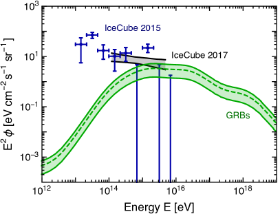
Figure 32: Diffuse neutrino flux per flavor $\nu_{\alpha}+\overline{\nu}_{\alpha}$ from GRBs Denton and Tamborra (2018a). The green band marked “GRBs” tracks the uncertainty of the local star-formation rate Strolger et al. (2015). Also shown is the IceCube neutrino flux from two data sets as in Fig. 31.

Figure 32 shows the diffuse neutrino emission per flavor ($\nu_{\alpha}+\overline{\nu}_{\alpha}$) and mass eigenstates from long-duration GRBs. It has been obtained according to the advanced model presented in Fig. 5 of Denton and Tamborra (2018a) which includes high-luminosity, low-luminosity, and choked GRBs. The astrophysical uncertainty is based on the error in the measurement of the local star-formation rate Strolger et al. (2015).

Short GRBs have typical luminosities similar to the ones of long high-luminosity GRBs but originate from compact binary mergers. The expected diffuse neutrino background from these sources is much smaller than the one from long-duration GRBs because of the merger distribution on cosmic scales Tamborra and Ando (2015). However, a sizable neutrino flux could be detected, if e.g. one invokes a large fraction of magnetars connected to these bursts Fang and Metzger (2017) or by exploiting the GRB extended emission that can potentially provide a larger target photon field Kimura et al. (2017).

XI.5 Blazars

AGNs are mainly powered by mass accretion onto supermassive black holes at the center of their host galaxies Padovani et al. (2017). AGNs are among the most luminous sources of electromagnetic radiation and have been proposed as powerful high-energy cosmic accelerators Murase (2017).

AGNs can be divided in radio-quiet and radio-loud objects. The latter are characterized by an emission from the jet and lobes that is especially prominent at radio wavelengths, whereas in radio-quiet objects the continuum emission comes from the core regions and the jet-related emission is weak. Radio-loud AGNs are promising cosmic accelerators and powerful neutrino sources.

Blazars are a special kind of loud AGNs with the jet pointing towards us. Blazars are characterized by extreme variability and strong emission over the entire electromagnetic spectrum. Blazars are divided into BL Lacertae objects (BL-Lacs) and flat spectrum radio quasars (FSRQs). These two categories have different optical spectra, the latter showing strong and broad emission lines and the former characterized by optical spectra with weak emission lines.

In the following, we will focus on neutrino production from blazars as they are expected to be rich neutrino factories. However, radio-quiet AGNs may also contribute to the diffuse neutrino background Murase (2017), although the neutrino production is affected by large uncertainties.

The photon spectrum of blazars is characterized by two broad bumps Padovani et al. (2017). The low-energy peak can occur at frequencies in the range 0.01–13 keV while the high-energy peak can be in the 0.4–400 MeV range. The low-energy emission of blazars comes from electron synchrotron radiation with the peak frequency being related to the maximum energy at which electrons can be accelerated. On the other hand, the origin of the high-energy emission is still under debate, it might originate from inverse Compton radiation or from the decay of pions generated by accelerated protons.

The electromagnetic spectrum evolves with the blazar luminosity, the so-called blazar sequence. The correspondent neutrino production occurs through ${p\gamma}$ interactions Atoyan and Dermer (2001); Protheroe (1997); in fact high-energy protons are accelerated through diffusive shock acceleration or stochastic acceleration in the jet. Protons then interact with synchrotron photons coming from non-thermal electrons that are co-accelerated in the jets. Given their abundance and brightness, the detection of neutrinos from stacked searches of blazars is statistically favored Feyereisen et al. (2017); Mertsch et al. (2017); Murase and Waxman (2016).

BL-Lacs produce up to 40–70$\%$ of the gamma-ray diffuse background in the 0.1–10 GeV range. Assuming that neutrinos are produced through $p\gamma$ interactions, the gamma-ray and neutrino luminosity from blazars may be connected through an efficiency factor $Y_{\nu\gamma}$ varying between 0.1 and 2, so that $L_{\nu}=Y_{\nu\gamma}L_{\gamma}$ Petropoulou et al. (2015).

To estimate the neutrino production from the blazar population, it is useful to rely on the blazar sequence. Although one can assume a distribution in the Lorentz factor of the jet, $\Gamma=10$ is here assumed as a representative value during a typical variability time of $10^{6}$ s. Cosmic rays undergo Fermi acceleration and acquire a power-law energy distribution $F_{p}(E_{p})=E_{p}^{-2}\exp{(-E_{p}/E_{\mathrm{max}})}$ with $E_{\mathrm{max}}$ the maximum energy that cosmic rays have in the source. In $p\gamma$ interactions, neutrinos carry about $5\%$ of the energy of the primary proton.

The target photon field is determined according to the blazar sequence Ghisellini et al. (2017). Beyond synchrotron and inverse Compton peaks present in the BL-Lac spectral energy distribution, FSRQs typically exhibit broad lines from atomic emission of the gas surrounding the accretion disk. By deriving the neutrino spectral energy distribution from the gamma-ray one and by relying on the blazar distribution at cosmological distances as from Fermi Ajello et al. (2014, 2012), Palladino et al. (2019) estimated the neutrino diffuse emission from blazars by imposing bounds on the non-observation of neutrino events from dedicated stacking searches and by assuming that the baryonic loading varies with the luminosity as a power law. The neutrino production from FSRQs is estimated to be about 30$\%$ of the BL-Lac one Padovani et al. (2015).

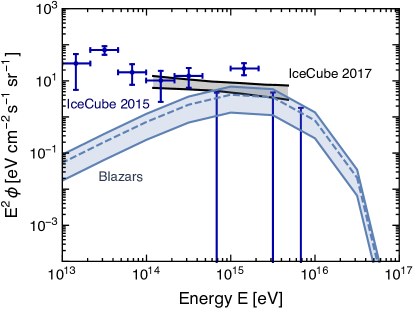
Figure 33: Diffuse neutrino background per flavor $\nu_{\alpha}+\overline{\nu}_{\alpha}$ from blazars Palladino et al. (2019). The blue band marked “Blazars” reproduces the possible variations ($1\sigma$) due to the uncertainties on the modeling of the neutrino emission. Also shown is the IceCube neutrino flux from two data sets as in Fig. 31. Thanks to A. Palladino for providing the data used in this figure.

Figure 33 shows the neutrino emission per flavor from blazars. It was obtained from Scenario 3 of Palladino et al. (2019); the $1\sigma$ uncertainty band includes all uncertainties due to the modeling of neutrino emission. Given the large uncertainties on the modeling of the diffuse neutrino emission from blazars, we refer the interested reader to Murase et al. (2014), Padovani et al. (2015), Aartsen et al. (2017b), Murase (2017), and Becker et al. (2005) for examples of alternative independent estimations of the neutrino emission.

In this Section, we focused on the diffuse neutrino emission from AGNs. However, IceCube recently reported hints for the detection of a dozen neutrino events along the direction of the blazar TXS 0506$+$056 Aartsen et al. (2018b, a). The interpretation of the neutrino energy distribution is currently in tension with the correspondent electromagnetic observations; however, if confirmed, this would correspond to the first detection of high-energy neutrinos from a cosmic source.

XI.6 Cosmogenic neutrinos

Ultra-high-energy cosmic rays (UHECRs) have energies up to $10^{20}$ eV; these are the particles with the highest energies observed in Nature Anchordoqui (2019). The sources producing them and the mechanisms behind their acceleration are unknown. Results from the Auger observatory suggest a light composition at 1 EeV which tends to become heavier with increasing energy Aab et al. (2014). Telescope Array (TA) data seem to confirm this trend, suggesting a mixed composition Abbasi et al. (2019).

On their way to Earth, UHECRs interact with radiation, specifically with the cosmic microwave background (CMB) and the extragalactic background light (EBL), which is the cosmic population of photons, e.g. in the infrared range. The energy spectrum of nucleons is mostly affected by the CMB because of pair production and photo-pion production, whereas the energy spectrum of heavier nuclei is affected by the EBL through pair production and photo-disintegration. Photo-pion interactions occur when nucleons ($N$) with Lorentz factor $\Gamma\geq 10^{10}$ interact with the CMB and pions are produced ($N+\gamma\rightarrow N+\pi^{0,\pm}$). For lower $\Gamma$, the same process can take place with the EBL. The strong flux suppression at high energies coming from the photo-pion production is responsible for the so-called Greisen-Zatsepin-Kuzmin (GZK) cutoff Greisen (1966); Zatsepin and Kuz’min (1966); Abbasi et al. (2008). Photodisintegration takes place when UHE nuclei are stripped by one or more nucleons by interacting with the CMB or EBL,

$$(A,Z)+\gamma\rightarrow(A-n,Z-n^{\prime})+nN\ ,$$ (61)

where $n$ and $n^{\prime}$ is the number of stripped nucleons and protons, respectively. Mesons produced in these interactions quickly decay and produce a flux of cosmogenic neutrinos Berezinsky and Zatsepin (1969); Heinze et al. (2016); Aloisio et al. (2015); Ahlers and Halzen (2012); Kotera et al. (2010); Allard et al. (2006). The $\beta$-decay of nucleons and nuclei from photo-disintegration can also lead to neutrino production. However, while neutrinos produced from pion decay have energies that are a few percent of the parent nucleus, those produced from $\beta$-decay carry less than one part per thousand of the parent nucleon’s energy.

The cosmogenic neutrino spectrum is also sensitive to the maximum UHECR energy and heavy composition at the source (or a weaker evolution of cosmic-ray sources) tends to produce a significantly lower cosmogenic neutrino flux Aloisio et al. (2015). The largest contribution is instead obtained if one assumes a proton source; this is, however, currently disfavored by Fermi data Alves Batista et al. (2019).

Interestingly, while the cosmic-ray spectrum is dominated by nearby sources, the neutrino flux will receive contributions up to cosmological scales. Moreover, the cosmogenic neutrino flux will also change according to the assumed source composition Aloisio et al. (2015); Ahlers and Halzen (2012).

Cosmogenic neutrinos have not been detected yet and IceCube has recently placed a new upper limit on this flux Aartsen et al. (2016b). This non-observation disfavors sources with a cosmological evolution that is stronger than the one predicted from the star-formation rate, such as AGNs Aartsen et al. (2016b) if one assumes a proton composition at the source. We show the predicted flux in Fig. 34, where we reproduce the results reported in Møller et al. (2019). Note that a lower cosmogenic neutrino flux may also be expected for mixed composition, see e.g. Alves Batista et al. (2019) and Kotera et al. (2010). The upper bounds obtained by ANITA and Auger are respectively shown in green and orange Ackermann et al. (2019). The next generation of radio facilities, such as the Giant Radio Array for Neutrino Detection (GRAND, see yellow curve in Fig. 34 for its projected sensitivity), and the Antarctic Ross Ice-Shelf ANtenna Neutrino Array (ARIANNA), will also be able to detect this flux, which contributes to the highest-energy range in the GUNS.

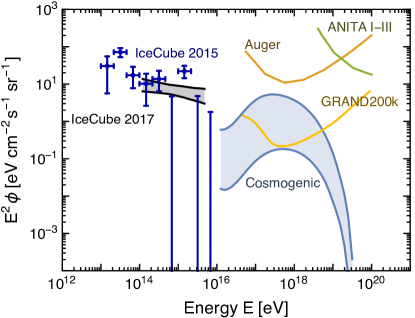
Figure 34: Cosmogenic neutrino flux per flavor $\nu_{\alpha}+\overline{\nu}_{\alpha}$ Møller et al. (2019). The bands reproduce the largest possible variations due to the uncertainties on the ultra-high-energy cosmic ray composition and source redshift evolution. The exclusion measurements of Auger, ANITA phase I-III, and projected 3-year sensitivity for GRAND (200,000-antenna array) are marked accordingly and shown respectively in orange, green, and yellow Ackermann et al. (2019); Álvarez-Muñiz et al. (2020). Also shown is the IceCube neutrino flux from two data sets as in Fig. 31.

XI.7 Future detection prospects

IceCube currently remains the only experiment that detects high-energy neutrinos from astrophysical sources. Considering further experimental efforts in the field of high-energy neutrino astronomy, IceCube-Gen2 Aartsen et al. (2014) is currently under planning. Another upcoming detector is KM3NeT Adrián-Martínez et al. (2016) which will have better sensitivity to Galactic sources.

For neutrino energies above the PeV range, GRAND Fang et al. (2018) is currently being designed and developed. ARIANNA Barwick et al. (2015), a hexagonal radio array, has already delivered first constraints on cosmogenic neutrinos. ARA, the Askaryan Radio Array, is currently being developed Allison et al. (2012). POEMMA Olinto et al. (2018) is being designed for the detection of cosmogenic tau neutrinos.

XII Discussion and Outlook

In analogy to the seminal Grand Unified Photon Spectrum of Ressell and Turner (1990), we have presented the Grand Unified Neutrino Spectrum (GUNS). This is a complete overview of the diffuse neutrino and antineutrino backgrounds at Earth ranging from the cosmic neutrino background in the meV range to cosmogenic neutrinos reaching up to $10^{18}$ eV.

The lowest-energy neutrinos are those from the cosmic neutrino background (CNB) and the $\bar{\nu}_{e}$’s from neutron and triton decay left over from big-bang nucleosynthesis. While these fluxes have not yet been detected, eventually the CNB may become experimentally accessible, depending on the actual neutrino mass spectrum. The lowest-energy neutrinos on our plot that have ever been observed are solar pp neutrinos down to 100 keV.

Neutrinos from nuclear reactions in the Sun and atmospheric neutrinos are the best measured and theoretically best understood sources. Most importantly, they have played a crucial role in detecting and exploring neutrino flavor conversion. Neutrinos from these sources continue to contribute to global fits of neutrino mixing parameters and in the search for possible non-standard effects in the neutrino sector.

In the few-MeV range, “antineutrino astronomy” is a field encompassing geological $\bar{\nu}_{e}$ sources as well as nuclear power reactors. Geoneutrinos have been observed for more than a decade, but thus far with somewhat limited statistics. It will take larger detectors to begin neutrino geology in earnest. In the long run, geoneutrino research will have practical implications, e.g. it could be employed for verification in the context of nuclear non-proliferation. Reactor neutrinos remain crucial sources for investigating neutrino mixing parameters or to study coherent neutrino scattering.

Geoneutrinos and neutrinos from reactors are relevant in the same energy range as the diffuse supernova neutrino background (DSNB). Likely the latter will be measured for the first time by the upcoming gadolinium-enhanced Super-Kamiokande detector and the JUNO scintillator detector, advancing the frontiers of neutrino astronomy to cosmological distances.

Atmospheric neutrinos partly overlap with the DSNB signal. Atmospheric neutrinos were crucial for the discovery of neutrino flavor conversions and to measure the neutrino mixing parameters. In the next future, a precise determination of the atmospheric neutrino flux will be fundamental for the detection of the DSNB to extract better constraints on the supernova population, as well to better discriminate the neutrinos of astrophysical origin in the range $1$–$50$ TeV.

Above some TeV, the neutrino backgrounds are far less explored. The IceCube neutrino telescope detects a flux of astrophysical neutrinos up to a few PeV, whose sources remain to be unveiled. At even higher energies, the detection of cosmogenic neutrinos will open a new window on the ultra-high-energy sky. Future experimental progress in this energy range will depend on increased statistics based on larger detection volumes as well as new detector technologies. An improved source identification in the context of multi-messenger studies will also contribute to better explore this part of the GUNS.

The GUNS plot reveals the neutrino potential of charting an extremely wide energy range. While astrophysical neutrinos have been instrumental for detecting flavor conversion, the mass and mixing parameters are now becoming a question of precision determination in laboratory experiments and global fits. The most exciting perspectives to learn about neutrino properties as well as their sources sit at the low- and high-energy tails of the GUNS. In particular, the branch of high and ultra-high energy neutrino astronomy is only in its infancy. The high-energy tail of the GUNS could unlock the secrets of the most energetic events occurring in our Universe, shed light on the origin of cosmic rays, and constrain standard and non-standard neutrino properties.

While we hope that our GUNS plot provides a useful overview of the global neutrino flux at Earth, we also anticipate that it will continue to require frequent updating both from new observations and new theoretical ideas and insights.

Appendix A Units and dimensions

We use natural units with $\hbar=c=k_{\rm B}=1$. The neutrino flux at Earth is shown integrated over all angles for all types of sources (point-like sources such as the Sun, diffuse such as geoneutrinos, or isotropic such as the DSNB), for example in units ${\rm cm}^{-2}~{}{\rm s}^{-1}~{}{\rm MeV}^{-1}$. On the other hand, in Secs. X and XI we follow the convention usually adopted in the neutrino-astronomy literature and show the fluxes in units ${\rm cm}^{-2}~{}{\rm s}^{-1}~{}{\rm GeV}^{-1}~{}{\rm sr}^{-1}$; i.e. the fluxes have been obtained by integrating over all angles and dividing by $4\pi$.

Multiplying the angle-integrated neutrino flux with the cross section of a target particle provides a differential detection rate per target particle $d\dot{n}/dE$. To take advantage of directional capabilities in some detectors one needs to restore, of course, the angular characteristic of the neutrino flux. Dividing our $4\pi$-integrated flux by the speed of light provides the number density at Earth per energy interval $dn/dE$, for example in units of ${\rm cm}^{-3}~{}{\rm MeV}^{-1}$, with the exception of nonrelativistic CNB neutrinos where the appropriate velocity has to be used. We mention these seemingly trivial details because sometimes one finds incorrect factors $4\pi$ in plots showing fluxes from both diffuse and point-like sources.

There is no ambiguity about the local number density, which may or may not have a nontrivial angular distribution. The $4\pi$-integrated flux can be interpreted as the number of neutrinos passing through a sphere of $1~{}{\rm cm}^{2}$ cross-sectional area per second. Other authors have used the picture of neutrinos passing from one side through a disk of $1~{}{\rm cm}^{2}$ area per second, which is a factor 1/4 smaller for an isotropic distribution such as the CNB. Such a definition would be appropriate, for example, for the detection of CMB photons by a horn antenna where we could only count the photons passing through the entrance cross section of the horn. Likewise, the emitted flux from a blackbody surface, as expressed by the Stefan-Boltzmann Law, is a factor 1/4 smaller than the energy density of isotropic blackbody radiation.

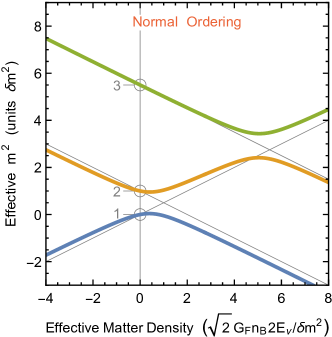
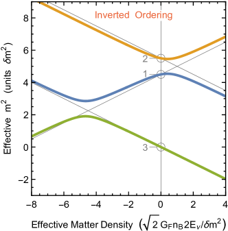
Figure 35: Effective neutrino masses in a medium in units of the solar mass difference $\delta m$. For this schematic plot, $m_{1}=0$, the atmospheric mass difference was chosen as $\Delta m^{2}=5\,\delta m^{2}$, and the mixing angles as $\sin^{2}\theta_{12}=0.30$ and $\sin^{2}\theta_{13}=0.01$. The electron and neutron densities were taken to be equal ($n_{e}=n_{n}=n_{B}/2$) appropriate for a medium consisting of ⁴He or ¹²C. A negative density is to be interpreted as a positive density for the energy levels of antineutrinos. At zero density the levels are the squared vacuum masses. The thin (gray) lines are the energy levels for vanishing mixing angles.

Appendix B Neutrino Mass Matrix

Neutrino fluxes from practically any source depend on flavor so that what arrives at the detector depends on flavor oscillations driven by neutrino masses and mixing. We restrict ourselves to a minimal scenario that includes only the three known species.

The weak-interaction neutrino fields $\nu_{\alpha}$ with $\alpha=e$, $\mu$ or $\tau$ are given in terms of fields with definite masses $\nu_{i}$ by a unitary transformation $\nu_{\alpha}=\sum_{i=1}^{3}{\sf U}_{\alpha i}\nu_{i}$, implying

$$|\nu_{\alpha}\rangle=\sum_{i=1}^{3}{\sf U}^{*}_{\alpha i}|\nu_{i}\rangle\quad\hbox{and}\quad|\overline{\nu}_{\alpha}\rangle=\sum_{i=1}^{3}{\sf U}_{\alpha i}|\overline{\nu}_{i}\rangle$$ (62)

for neutrino and antineutrino single-particle states Giunti and Kim (2007). The mixing matrix is conventionally expressed in terms of three two-flavor mixing angles $0\leq\theta_{ij}<\pi/2$ and a CP-violating phase $0\leq\delta<2\pi$ in the form

$${\sf U} =\hbox{\footnotesize$\begin{pmatrix}1&0&0\\ 0&c_{23}&s_{23}\\ 0&-s_{23}&c_{23}\end{pmatrix}\begin{pmatrix}c_{13}&0&s_{13}e^{-i\delta}\\ 0&1&0\\ -s_{13}e^{i\delta}&0&c_{12}\end{pmatrix}\begin{pmatrix}c_{12}&s_{12}&0\\ -s_{12}&c_{12}&0\\ 0&0&1\end{pmatrix}$}$$

$$= \hbox{\footnotesize$\begin{pmatrix}c_{12}c_{13}&s_{12}c_{13}&s_{13}e^{-i\delta}\\ -s_{12}c_{23}-c_{12}s_{23}s_{13}e^{i\delta}&c_{12}c_{23}-s_{12}s_{23}s_{13}e^{i\delta}&s_{23}c_{13}\\ s_{12}s_{23}-c_{12}c_{23}s_{13}e^{i\delta}&-c_{12}s_{23}-s_{12}c_{23}s_{13}e^{i\delta}&c_{23}c_{13}\end{pmatrix}$},$$

where $c_{ij}=\cos\theta_{ij}$ and $s_{ij}=\sin\theta_{ij}$. We have left out a factor ${\rm diag}(1,e^{i\alpha_{21}/2},e^{i\alpha_{31}/2})$ of Majorana phases that are important, for example, in neutrinoless double-beta decay, but not for flavor oscillations.

Table 5: Neutrino mixing angles according to Capozzi et al. (2018), very similar to those of de Salas et al. (2018) and Esteban et al. (2017).

	Normal Ordering		Inverted Ordering
	Best fit	1$\sigma$ range	Best fit	1$\sigma$ range
$\sin^{2}\theta_{12}$	0.304	0.291–0.318	0.303	0.290–0.317
$\sin^{2}\theta_{13}$	0.0214	0.0207–0.0223	0.0218	0.0211–0.0226
$\sin^{2}\theta_{23}$	0.551	0.481–0.570	0.557	0.533–0.574
$\delta/\pi$	1.32	1.14–1.55	1.52	1.37–1.66

The best-fit mixing angles determined from global fits of all flavor oscillation data are given in Table 5. Within uncertainties, the octant of $\theta_{23}$ remains unknown, i.e., if $\sin^{2}\theta_{23}$ is larger or smaller than $1/2$. CP violation is favored, but the range of allowed $\delta$ remains large.

With the results of Table 5 for normal mass ordering one finds the matrix of mixing probabilities, which is the same for $\nu$ and $\overline{\nu}$,

$$\bigl{(}|{\sf U}_{\alpha i}|^{2}\bigr{)}=\begin{pmatrix}0.681^{+0.013}_{-0.014}&0.297^{+0.014}_{-0.013}&0.0214^{+0.0009}_{-0.0007}\\[4.30554pt] 0.109^{+0.074}_{-0.035}&0.352^{+0.080}_{-0.065}&0.539^{+0.019}_{-0.069}\\[4.30554pt] 0.210^{+0.040}_{-0.073}&0.351^{+0.067}_{-0.082}&0.439^{+0.069}_{-0.019}\end{pmatrix}.$$ (64)

The uncertainties correspond to the maximal and minimal values within the $1\sigma$ ranges shown in Table 5. Of course, the rows and columns of this matrix of probabilities always have to add up to 1. The first row, for example, means that a produced $\nu_{e}$ has a 68% chance to be a $\nu_{1}$, 30% to be $\nu_{2}$, and 2% to be $\nu_{3}$. The mass eigenstates are conventionally numbered such that the probabilities in the first row appear in declining order, i.e., according to the $\nu_{i}$ admixtures to $\nu_{e}$.

The matrix ${\sf U}$ being unitary, its inverse ${\sf U}^{-1}$, which allows us to express mass states in terms of flavor states, is identical with its conjugate transpose ${\sf U}^{\dagger}$. Therefore, the probabilities for finding a given mass eigenstates in any of the flavors correspond to the columns of Eq. (64). For example, the last column tells us that a $\nu_{3}$, for example in the cosmic neutrino background, has a 2% chance of being $\nu_{e}$, a 54% chance of being $\nu_{\mu}$, and 44% of being $\nu_{\tau}$, and analogous for the other columns.

The numbering convention of mass states leaves open the ordering of the mass values. The matter effect on flavor conversion in the Sun implies $m_{1}<m_{2}$. The atmospheric ordering may be normal with $m_{1}<m_{2}<m_{3}$ or inverted with $m_{3}<m_{1}<m_{2}$. Global fits somewhat prefer normal ordering. The probability matrix for inverted ordering is similar to Eq. (64) within the shown uncertainties.

Flavor oscillations of relativistic neutrinos are driven by the squared-mass differences. We express the mass spectrum in terms of the parameters Capozzi et al. (2018)

$$\kern-20.00003pt\delta m^{2} = m_{2}^{2}-m_{1}^{2}\kern 27.0pt{}=73.4~{}{\rm meV}^{2}\,,$$ (65a)

$$\kern-20.00003pt\Delta m^{2} = m_{3}^{2}-\frac{m_{1}^{2}+m_{2}^{2}}{2}=\pm 2.45\times 10^{3}~{}{\rm meV}^{2}\,,$$ (65b)

where normal ordering corresponds to $\Delta m^{2}>0$, inverted ordering to $\Delta m^{2}<0$. The nominal $1\sigma$ range of the measured values is 1.4 and 2.2%, respectively. The small mass splitting $\delta m^{2}$ is also called the solar mass difference because it drives solar neutrino conversion, whereas $\Delta m^{2}$ is the atmospheric one. Often the atmospheric splitting is instead identified with either $m_{3}^{2}-m_{2}^{2}$ or $m_{1}^{2}-m_{3}^{2}$, depending on the mass ordering, which however is a less practical convention.

Direct laboratory limits on the unknown overall mass scale of approximately 2 eV derive from the electron endpoint spectrum in tritium $\beta$ decay Tanabashi et al. (2018). The KATRIN experiment is expected to improve the sensitivity to approximately 0.2 eV in the near future Arenz et al. (2018).

Cosmological data constrain the fraction of hot dark matter, implying 95% C.L. limits $\sum m_{\nu}<0.11$–$0.68~{}{\rm eV}$, depending on the used data and cosmological model Ade et al. (2016); Aghanim et al. (2020); Lesgourgues and Verde (2018). Near-future surveys should be able to set a lower limit, i.e., provide a neutrino-mass detection Lesgourgues and Verde (2018). Of course, these results have to be interpreted with the usual caveats about cosmological assumptions and possible unrecognized systematics.

The neutrino signal from the next nearby supernova can provide a 95% C.L. time-of-flight limit of 0.14 eV if the emission shows few-millisecond time variations caused by hydrodynamic instabilities as suggested by 2D and 3D simulations Ellis et al. (2012).

Searches for neutrinoless double beta decay are only sensitive to Majorana masses, and specifically to the combination $\langle m_{\nu}\rangle=\bigl{|}\sum_{i=1}^{3}{\sf U}_{ei}^{2}m_{i}\bigr{|}$. Current limits are on the level of 0.11–0.52 eV, depending on isotope and on uncertainties of the nuclear matrix elements Tanabashi et al. (2018).

Appendix C Neutrino Mixing in Matter

When they propagate in matter, neutrinos experience a flavor-dependent potential caused by the electroweak interaction. In a normal medium, consisting of nuclei and electrons, it is

$$V_{\rm weak}=\pm\sqrt{2}G_{\rm F}n_{B}\times\begin{cases}Y_{e}-Y_{n}/2,&\mbox{for $\nu_{e}$},\\ -Y_{n}/2,&\mbox{for $\nu_{\mu,\tau}$},\end{cases}$$ (66)

where $n_{B}$ is the baryon density, $Y_{e}=n_{e}/n_{B}$ the net electron fraction per baryon (electrons minus positrons), and $Y_{n}=n_{n}/n_{B}$ the neutron fraction. The upper sign is for $\nu$, the lower sign for $\overline{\nu}$. Equivalently, we can use a nominally negative baryon density to denote the $\overline{\nu}$ potential. Radiative corrections actually provide a small difference between the $\nu_{\mu}$ and $\nu_{\tau}$ potentials Botella et al. (1987); Mirizzi et al. (2009), as does the possible presence of muons in a supernova core Bollig et al. (2017). We also ignore background neutrinos which complicate neutrino propagation in the form of collective flavor evolution Duan et al. (2010).

The flavor of a neutrino of fixed energy $E$ evolves as a function of distance $z$ as $i\partial_{z}\Psi=({\sf H}_{0}+{\sf V})\Psi$, where $\Psi$ is a three-vector of flavor amplitudes, whereas antineutrinos evolve as $i\partial_{z}\overline{\Psi}=({\sf H}_{0}^{*}-{\sf V})\overline{\Psi}$. In the ultrarelativistic limit, the mass contribution in the flavor basis is

$${\sf H}_{0}=\frac{1}{2E}{\sf U}\begin{pmatrix}m_{1}^{2}&0&0\\ 0&m_{2}^{2}&0\\ 0&0&m_{3}^{2}\end{pmatrix}{\sf U}^{\dagger}$$ (67)

and the matrix of potential energies is

$${\sf V}=\sqrt{2}G_{\rm F}\begin{pmatrix}n_{e}-n_{n}/2&0&0\\ 0&-n_{n}/2&0\\ 0&0&-n_{n}/2\end{pmatrix}.$$ (68)

Without flavor mixing, the in-medium dispersion relation in the relativistic limit is given by the effective masses $m_{\rm eff}^{2}=m^{2}+V_{\rm weak}2E$, shown as thin gray lines in Fig. 35 for a schematic choice of mass and mixing parameters. A nominally negative density is used to show the energy levels for antineutrinos. The background medium is taken to have equal densities of electrons and neutrons as would be the case for ⁴He or ¹²C. For a different composition, the lines acquire a different slope caused by the common neutral-current potential for all flavors.

For nonvanishing mixing angles, the effective masses are obtained by diagonalizing ${\sf H}_{0}+{\sf V}$, which is achieved by a unitary matrix ${\sf U}_{\rm M}$ such that

$${\sf M}_{\rm eff}^{2} = \begin{pmatrix}m_{1,\rm eff}^{2}&0&0\\ 0&m_{2,\rm eff}^{2}&0\\ 0&0&m_{3,\rm eff}^{2}\end{pmatrix}$$ (69)

$$= {\sf U}^{\dagger}_{\rm M}\big{(}{\sf U}{\sf M}^{2}{\sf U}^{\dagger}+2E\,{\sf V}\big{)}{\sf U}_{\rm M}.$$

For antineutrinos, one substitutes ${\sf V}\to-{\sf V}$ and $\delta\to-\delta$, the latter equivalent to ${\sf U}\to{\sf U}^{*}$. Notice that $m_{i,\rm eff}^{2}$ can be negative because it is just a formal way for writing the in-medium energy levels. In Fig. 35, the $m_{i,\rm eff}^{2}$ are shown as thick colored lines. Notice that $\theta_{23}$ and $\delta$ do not enter if the $\nu_{\mu}$ and $\nu_{\tau}$ potentials are equal — otherwise there will be a third level crossing. Notice also that asymptotically the colored lines have a nonvanishing offset relative to the gray lines.

Of particular interest is the case of neutrinos produced at high density in the interior of a star which then propagate all the way to the surface. If the propagation is adiabatic (and this is the case for solar and supernova neutrinos), a state originally in a propagation eigenstate emerges as such. So we should decompose the flavor states at the point of production into local propagation states which then connect to vacuum mass states at the stellar surface (MSW effect). In sufficiently dense matter, the propagation eigenstates coincide with interaction eigenstates. In Fig. 35 (normal ordering), a $\nu_{e}$ produced at very high density corresponds to the largest $m_{\rm eff}^{2}$, i.e., the thick green line. Following this line to zero density (vacuum), we see that a produced $\nu_{e}$ will emerge as the mass eigenstate $\nu_{3}$. Conversely, a $\overline{\nu}_{e}$ (large negative density) is on the blue line and thus emerges as $\nu_{1}$. A detailed discussion of all such cases, relevant in the supernova context, was provided by Dighe and Smirnov (2000).

Often the flavor-diagonal contribution to ${\sf V}$ provided by neutrons is not included because it drops out of the oscillation equation. In this case, and using the best-fit mixing parameters in normal ordering from Table 5, the same plot of $m_{i,\rm eff}^{2}$ is shown in Fig. 36 (top). In the Sun, the central density is $150~{}{\rm g}~{}{\rm cm}^{-3}$ with $Y_{e}=0.681$, corresponding to $n_{e}=6.14\times 10^{25}~{}{\rm cm}^{-3}=4.72\times 10^{11}~{}{\rm eV}^{3}$ and thus to $V_{e}=7.8\times 10^{-12}~{}{\rm eV}$, where

$$V_{e}=\sqrt{2}G_{\rm F}n_{e}.$$ (70)

With $E=18.8~{}{\rm MeV}$, near the highest solar $\nu_{e}$ energy, one finds $V_{e}2E<233~{}{\rm meV}^{2}=4.0~{}\delta m^{2}$, indicated by a vertical dashed line in Fig. 36.

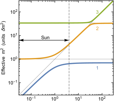
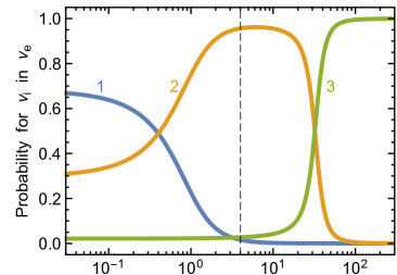
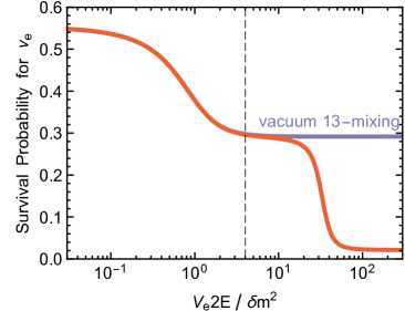
Figure 36: Neutrino mixing in matter. Top: Effective masses-squared, $m_{i,{\rm eff}}^{2}$ with $i=1$, 2 or 3, in units of the solar value $\delta m^{2}$. The neutron contribution, which is flavor diagonal, has been ignored. The mixing parameters are the best-fit values in normal ordering from Table 5. In the Sun, the maximum on the horizontal axis is 4.0 (vertical dashed line), corresponding to $n_{e}=6.14\times 10^{25}~{}{\rm cm}^{-3}$ at the solar center and the largest $\nu_{e}$ energy of $E=18.8$ MeV. Middle: Probability of a produced $\nu_{e}$ to be in the propagation eigenstates 1, 2 or 3, corresponding to $|{\sf U}^{\rm M}_{ei}|^{2}$. Bottom: Probability of a produced $\nu_{e}$, after adiabatic propagation, to be measured as a $\nu_{e}$ according to Eq. (71). For solar conditions (left of the dashed line), ignoring the matter effect on 13–mixing yields an excellent approximation.

The probability for a $\nu_{e}$ that was produced in the medium to be found in any of the propagation eigenstates $i$ is $P_{ei}^{\rm M}=|{\sf U}_{ei}^{\rm M}|^{2}$, shown in Fig. 36 (middle) from a numerical solution for ${\sf U}_{\rm M}$ using the best-fit mixing parameters. At zero density, the $P_{ei}$ correspond to the top row in the matrix of Eq. (64). At very high density, $\nu_{e}$ essentially coincides with $\nu_{3}$, so after adiabatic propagation it would emerge in the third mass eigenstate as mentioned earlier.

Neutrinos propagating from a distant source decohere into mass eigenstates, so for example the $\nu_{e}$ produced in the Sun arrive with probabilities $P_{ei}$ in the different mass eigenstates, depending on the exact point of production and depending on their energy. A detector which is only sensitive to $\nu_{e}$ projects from each of the $\nu_{i}$ fluxes the $\nu_{e}$ component, corresponding to the probability $|{\sf U}_{ei}|^{2}$, so the $\nu_{e}$ survival probability is

$$P_{ee}=\sum_{i=1}^{3}\bigl{|}{\sf U}_{ei}^{\rm M}\bigr{|}^{2}\,\bigl{|}{\sf U}_{ei}\bigr{|}^{2},$$ (71)

shown as a red line in Fig. 36 (bottom). For neutrinos produced at very low density and/or with very low energies, this is, using Eq. (B)

$$P_{ee}^{\rm vac}=(c_{12}^{4}+s_{12}^{4})c_{13}^{4}+s_{13}^{4}=0.553,$$ (72)

where the numerical value is for the best-fit mixing angles in normal mass ordering.

The mass differences are hierarchical, $\delta m^{2}\ll\Delta m^{2}$, allowing for an approximate determination of ${\sf U}_{\rm M}$ Denton et al. (2016); Ioannisian and Pokorski (2018). Writing it in the form of Eq. (B), one finds for the in-medium mixing angles $\theta_{23}^{\rm M}=\theta_{23}$, $\delta^{\rm M}=\delta$, and

$$2\theta_{12}^{\rm M} = {\rm ArcTan}\left(\cos 2\theta_{12}{-}\epsilon_{\odot},\cos\theta_{13}^{\prime}\sin 2\theta_{12}\right),$$ (73a)

$$2\theta_{13}^{\rm M} = {\rm ArcTan}\left(\cos 2\theta_{13}{-}\epsilon_{\rm a},\sin 2\theta_{13}\right),$$ (73b)

where $\theta_{13}^{\prime}=\theta_{13}^{\rm M}-\theta_{13}$. Here, $\alpha={\rm ArcTan}(x,y)$ is an angle such that $\sin\alpha=y/\sqrt{x^{2}+y^{2}}$ and $\cos\alpha=x/\sqrt{x^{2}+y^{2}}$. Further,

$$\epsilon_{\odot} = \frac{2EV_{e}}{\delta m^{2}}\,\left(\cos^{2}\theta_{13}^{\rm M}+\frac{\sin^{2}\theta_{13}^{\prime}}{\epsilon_{\rm a}}\right),$$ (74a)

$$\epsilon_{\rm a} = \frac{2EV_{e}}{m_{3}^{2}-m_{1}^{2}-\delta m^{2}\sin^{2}\theta_{12}},$$ (74b)

where $\epsilon_{\rm a}<0$ for inverted mass ordering ($m_{3}^{2}<m_{1}^{2}$). The approximate analytic probabilities $|U^{\rm M}_{ei}|^{2}$ agree very well with the numerical values shown in the middle panel of Fig. 36. The agreement is better than $10^{-3}$ except for $|U^{\rm M}_{e1}|^{2}$ where above 10 on the horizontal axis the analytic probability falls off faster than the numerical one. The differences between analytic and numerical solutions are essentially irrelevant on a level of precision where we have ignored radiative corrections to the weak potential.

The maximum value of $2EV_{e}$ in the Sun is small compared with $m_{3}^{2}-m_{1}^{2}$, so for solar conditions we may neglect the matter effect on $\theta_{13}$. In this case ${\sf U}_{\rm M}$ is given in terms of the vacuum mixing angles except for

$$2\theta_{12}^{\rm M}={\rm ArcTan}\left(\cos 2\theta_{12}{-}\epsilon_{\odot},\sin 2\theta_{12}\right)$$ (75)

with

$$\epsilon_{\odot}=\frac{2EV_{e}}{\delta m^{2}}\,\cos^{2}\theta_{13}\,.$$ (76)

In this case, the probability for a produced $\nu_{e}$ to be found in any of the three propagation eigenstates is

$$P_{e1} = \cos^{2}\theta_{13}\,\cos^{2}\theta_{12}^{\rm M},$$ (77a)

$$P_{e2} = \cos^{2}\theta_{13}\,\sin^{2}\theta_{12}^{\rm M},$$ (77b)

$$P_{e3} = \sin^{2}\theta_{13}\,.$$ (77c)

The $\nu_{e}$ survival probability is

$$P_{ee}=\frac{1+\cos 2\theta_{12}\cos 2\theta_{12}^{\rm M}}{2}\,\cos^{4}\theta_{13}+\sin^{4}\theta_{13}$$ (78)

marked as “vacuum 13–mixing” in Fig. 36 (bottom). The best-fit value $\sin^{2}\theta_{13}=0.0214$ implies that we can safely neglect $\sin^{4}\theta_{13}$, whereas $\cos^{4}\theta_{13}=0.958$ deviates significantly from 1.

Appendix D Constructing the GUNS plot

For those wishing to construct their own version of the GUNS plot of Fig. 1 we here provide the exact input information that we have used. We also provide numerical tables, enclosed as ancillary files in the arXiv repository, that can be used for this purpose.

The GUNS plot shows the sum over all flavor or mass eigenstates for neutrinos (solid lines) and antineutrino (dashed lines). Notice that the uncertainty bands for atmospheric, IceCube, and cosmogenic neutrinos are only indicative because in the literature one finds $E^{2}\phi_{\nu}$ and its uncertainty, so the uncertainty of $\phi_{\nu}$ also depends on the energy uncertainty in a steeply falling spectrum.

The IceCube and cosmogenic fluxes in Fig. 1 can be compared to the corresponding figures in the main text by multiplying the curves in Fig. 1 with ${E^{2}/4\pi\times 2/3}$. In Fig. 1 we show an angle-integrated flux, hence the factor $1/4\pi$ to arrive the traditional fluxes per solid angle shown in high-energy neutrino astronomy. The factor 1/3 translates the sum over all flavors to a single-flavor flux, assuming flavor equipartition arriving at Earth. The factor 2 sums over neutrinos plus antineutrinos.

D.1 Cosmic neutrino background

For the CNB we assume the neutrino masses of Eq. (2). We show blackbody radiation for one mass eigenstate, following Eq. (6) and listed as a numerical table in the file CNB.dat. In addition there are two line sources (expressed in units of $\rm cm^{-2}\,s^{-1}$ in the upper panel and in units of $\rm eV\,cm^{-2}\,s^{-1}$ in the lower panel), corresponding to the $m_{2}$ and $m_{3}$ mass eigenstates. The normalization is given by the integral of Eq. (2). The line fluxes can be found in the file CNB-lines.dat.

D.2 Neutrinos from big-bang nucleosynthesis

For neutrinos produced by the decay of neutrons and tritium during big-bang nucleosynthesis we adopt the fluxes found in Ivanchik and Yurchenko (2018). The tables BBN-neutron.dat and BBN-tritium.dat are courtesy of these authors.

D.3 Thermal neutrinos from the Sun

For neutrinos produced by thermal processes in the Sun we use the flux computed in Vitagliano et al. (2017), see the table Sun-thermal.dat.

D.4 Solar neutrinos from nuclear reactions

The solar neutrino flux is equivalent to Fig. 7. The flux from the pp chains and CNO cycle is given (except for hep) by the measurements shown in Table 1. For the CNO and hep fluxes the range is bracketed by the lowest AGSS09 and highest GS98 predictions. The flux is given by the sum of all the processes contributing to the solar neutrino flux, which can be found in Sun-nuclear-B8.dat, Sun-nuclear-N13.dat, Sun-nuclear-O15.dat, Sun-nuclear-hep.dat, and Sun-nuclear-pp.dat. The lines due to electron capture are provided in Sun-lines.dat.

D.5 Geoneutrinos

The average geoneutrino flux is the sum over the different processes shown in Fig. 13. We have used the publicly available data of Enomoto (2005). The flux is tabulated in Geoneutrinos.dat.

D.6 Reactor neutrinos

The reactor $\overline{\nu}_{e}$ flux is tabulated in Reactor.dat for the example of 140 MW thermal power and a detector at the close distance of 81 m. We assume that each reaction release $205\rm\,MeV$ and the number of neutrinos per reaction per unit energy is obtained as in Fig. 15 (see also main text). Notice that this is not equivalent to the JOYO detector example shown in Fig. 16. The choice of this reactor-detector system is arbitrary, and can be rescaled accordingly. Of course, what to show on the GUNS plot is somewhat arbitrary because reactor fluxes depend most sensitively on location of all GUNS components.

D.7 Diffuse supernovae neutrino background

The DSNB neutrino and antineutrino fluxes can be found in DSNB.dat. The table has five entries: energy, lower and upper bound for the neutrino flux, and lower and upper bound for the antineutrino one. Each flux was calculated as ${\phi_{\nu_{e}}+2\phi_{\nu_{x}}}$. The uncertainty band was obtained considering the simplified scenario discussed in the main text for the supernova masses (9.6, 27, 40) $M_{\odot}$ with (50,20,21)% and (59,32,9)% for the supernova models.

D.8 Atmospheric neutrinos

Atmospheric neutrino and antineutrino fluxes can be found in Atmospheric.dat, in each case the sum of the electron and muon flavored fluxes. The low-energy points ($\lesssim 100\,\text{MeV}$) are from the tables of Battistoni et al. (2005), while the energy range ($100\,\text{MeV}\lesssim E\lesssim 1\rm\,TeV$) is from the publicly available results of Honda et al. (2015). We show the flux for average solar activity at the Kamioka site. The high-energy ($E\gtrsim 1\rm\,TeV$) flux is taken from Richard et al. (2016) and Aartsen et al. (2015c).

D.9 IceCube neutrinos

The high-energy astrophysical neutrino flux (in units $10^{-20}\,\rm eV^{-1}\,cm^{-2}\,s^{-1}$), as measured by IceCube, is tabulated in IceCube.dat with an upper and lower bound of the expected cosmogenic flux. These data are taken from the high-energy events analysis of Aartsen et al. (2017c).

D.10 Cosmogenic neutrinos

Cosmogenic neutrinos are tabulated in three columns in Cosmogenic.dat, i.e., energy and fluxes (in units $10^{-30}\,\rm eV^{-1}\,cm^{-2}\,s^{-1}$) for two models of the primary cosmic-ray composition, taken to represent an upper and a lower bound. The data used in the figure have been estimated in Møller et al. (2019).

D.11 Overall GUNS plot

As an example for constructing the GUNS plot from these data files we also include a Mathematica notebook named Produce-your-GUNS.nb that can be used to create other variations of this plot.

References

- Aab et al. (2014) Aab, A., et al. (Pierre Auger) 2014, Depth of maximum of air-shower profiles at the Pierre Auger Observatory. II. Composition implications, Phys. Rev. D 90, 122006, arXiv:1409.5083 .
- Aartsen et al. (2013a) Aartsen, M. G., et al. (IceCube) 2013a, Evidence for high-energy extraterrestrial neutrinos at the IceCube detector, Science 342, 1242856, arXiv:1311.5238 .
- Aartsen et al. (2013b) Aartsen, M. G., et al. (IceCube) 2013b, First observation of PeV-energy neutrinos with IceCube, Phys. Rev. Lett. 111, 021103, arXiv:1304.5356 .
- Aartsen et al. (2014) Aartsen, M. G., et al. (IceCube) 2014, IceCube-Gen2: A vision for the future of neutrino astronomy in Antarctica, arXiv:1412.5106 .
- Aartsen et al. (2015a) Aartsen, M. G., et al. (IceCube) 2015a, A combined maximum-likelihood analysis of the high-energy astrophysical neutrino flux measured with IceCube, Astrophys. J. 809, 98, arXiv:1507.03991 .
- Aartsen et al. (2015b) Aartsen, M. G., et al. (IceCube) 2015b, Atmospheric and astrophysical neutrinos above 1 TeV interacting in IceCube, Phys. Rev. D 91, 022001, arXiv:1410.1749 .
- Aartsen et al. (2015c) Aartsen, M. G., et al. (IceCube) 2015c, Development of a general analysis and unfolding scheme and its application to measure the energy spectrum of atmospheric neutrinos with IceCube, Eur. Phys. J. C 75, 116, arXiv:1409.4535 .
- Aartsen et al. (2015d) Aartsen, M. G., et al. (IceCube) 2015d, Measurement of the atmospheric spectrum with IceCube, Phys. Rev. D 91, 122004, arXiv:1504.03753 .
- Aartsen et al. (2016a) Aartsen, M. G., et al. (IceCube) 2016a, An all-sky search for three flavors of neutrinos from gamma-ray bursts with the IceCube neutrino observatory, Astrophys. J. 824, 115, arXiv:1601.06484 .
- Aartsen et al. (2016b) Aartsen, M. G., et al. (IceCube) 2016b, Constraints on ultrahigh-energy cosmic-ray sources from a search for neutrinos above 10 PeV with IceCube, Phys. Rev. Lett. 117, 241101, Erratum: Phys. Rev. Lett. 119 (2017) 259902, arXiv:1607.05886 .
- Aartsen et al. (2016c) Aartsen, M. G., et al. (IceCube) 2016c, Observation and characterization of a cosmic muon neutrino flux from the northern hemisphere using six years of IceCube data, Astrophys. J. 833, 3, arXiv:1607.08006 .
- Aartsen et al. (2016d) Aartsen, M. G., et al. (IceCube, Pierre Auger, Telescope Array) 2016d, Search for correlations between the arrival directions of IceCube neutrino events and ultrahigh-energy cosmic rays detected by the Pierre Auger Observatory and the Telescope Array, JCAP 1601, 037, arXiv:1511.09408 .
- Aartsen et al. (2017a) Aartsen, M. G., et al. (IceCube) 2017a, Extending the search for muon neutrinos coincident with gamma-ray bursts in IceCube data, Astrophys. J. 843, 112, arXiv:1702.06868 .
- Aartsen et al. (2017b) Aartsen, M. G., et al. (IceCube) 2017b, The contribution of Fermi-2LAC blazars to the diffuse TeV-PeV neutrino flux, Astrophys. J. 835, 45, arXiv:1611.03874 .
- Aartsen et al. (2017c) Aartsen, M. G., et al. (IceCube) 2017c, The IceCube Neutrino Observatory — Contributions to ICRC 2017 Part II: Properties of the atmospheric and astrophysical neutrino flux, arXiv:1710.01191 .
- Aartsen et al. (2018a) Aartsen, M. G., et al. (Liverpool Telescope, MAGIC, H.E.S.S., AGILE, Kiso, VLA/17B-403, INTEGRAL, Kapteyn, Subaru, HAWC, Fermi-LAT, ASAS-SN, VERITAS, Kanata, IceCube, Swift NuSTAR) 2018a, Multimessenger observations of a flaring blazar coincident with high-energy neutrino IceCube-170922A, Science 361, eaat1378, arXiv:1807.08816 .
- Aartsen et al. (2018b) Aartsen, M. G., et al. (IceCube) 2018b, Neutrino emission from the direction of the blazar TXS 0506+056 prior to the IceCube-170922A alert, Science 361, 147, arXiv:1807.08794 .
- Aartsen et al. (2019) Aartsen, M. G., et al. (IceCube) 2019, Measurement of atmospheric tau neutrino appearance with IceCube DeepCore, Phys. Rev. D 99, 032007, arXiv:1901.05366 .
- Abazajian et al. (2012) Abazajian, K., et al. 2012, Light sterile neutrinos: A White Paper, arXiv:1204.5379 .
- Abbasi et al. (2012) Abbasi, R., et al. (IceCube) 2012, The design and performance of IceCube DeepCore, Astropart. Phys. 35, 615, arXiv:1109.6096 .
- Abbasi et al. (2008) Abbasi, R. U., et al. (HiRes) 2008, First observation of the Greisen-Zatsepin-Kuzmin suppression, Phys. Rev. Lett. 100, 101101, arXiv:astro-ph/0703099 .
- Abbasi et al. (2019) Abbasi, R. U., et al. (Telescope Array) 2019, Mass composition of ultrahigh-energy cosmic rays with the Telescope Array Surface Detector data, Phys. Rev. D 99, 022002, arXiv:1808.03680 .
- Abbott et al. (2016) Abbott, B. P., et al. (LIGO Scientific and Virgo) 2016, GW151226: Observation of gravitational waves from a 22-solar-mass binary black hole coalescence, Phys. Rev. Lett. 116, 241103, for further detections and latest developments see LIGO and Virgo homepage, arXiv:1606.04855 .
- Abdurashitov et al. (2009) Abdurashitov, J. N., et al. (SAGE) 2009, Measurement of the solar neutrino capture rate with gallium metal. III: Results for the 2002–2007 data-taking period, Phys. Rev. C 80, 015807, arXiv:0901.2200 .
- Abe et al. (2016) Abe, K., et al. (Super-Kamiokande) 2016, Solar neutrino measurements in Super-Kamiokande-IV, Phys. Rev. D 94, 052010, arXiv:1606.07538 .
- Abe et al. (2018) Abe, K., et al. (Hyper-Kamiokande) 2018, Hyper-Kamiokande Design Report, arXiv:1805.04163 .
- Abe et al. (2011) Abe, S., et al. (KamLAND) 2011, Measurement of the 8B solar neutrino flux with the KamLAND liquid scintillator detector, Phys. Rev. C 84, 035804, arXiv:1106.0861 .
- Abe et al. (2012) Abe, Y., et al. (Double Chooz) 2012, Indication of reactor disappearance in the Double Chooz experiment, Phys. Rev. Lett. 108, 131801, arXiv:1112.6353 .
- Acciarri et al. (2016) Acciarri, R., et al. (DUNE) 2016, Long-Baseline Neutrino Facility (LBNF) and Deep Underground Neutrino Experiment (DUNE). Conceptual Design Report. Volume 4: The DUNE detectors at LBNF, arXiv:1601.02984 .
- Achar et al. (1965) Achar, C. V., et al. 1965, Detection of muons produced by cosmic ray neutrinos deep underground, Phys. Lett. 18, 196.
- Ackermann et al. (2012) Ackermann, M., et al. (Fermi-LAT) 2012, GeV observations of star-forming galaxies with Fermi LAT, Astrophys. J. 755, 164, arXiv:1206.1346 .
- Ackermann et al. (2016) Ackermann, M., et al. (Fermi-LAT) 2016, Resolving the extragalactic -ray background above 50 GeV with the Fermi Large Area Telescope, Phys. Rev. Lett. 116, 151105, arXiv:1511.00693 .
- Ackermann et al. (2019) Ackermann, M., et al. 2019, Astrophysics uniquely enabled by observations of high-energy cosmic neutrinos, Bull. Am. Astron. Soc. 51, 185, arXiv:1903.04334 .
- Adams et al. (2013) Adams, S. M., C. S. Kochanek, J. F. Beacom, M. R. Vagins, and K. Z. Stanek 2013, Observing the next Galactic supernova, Astrophys. J. 778, 164, arXiv:1306.0559 .
- Adams et al. (2017) Adams, S. M., C. S. Kochanek, J. R. Gerke, and K. Z. Stanek 2017, The search for failed supernovae with the Large Binocular Telescope: Constraints from 7 yr of data, Mon. Not. Roy. Astron. Soc. 469, 1445, arXiv:1610.02402 .
- Adamson et al. (2011) Adamson, P., et al. (MINOS) 2011, Measurement of the neutrino mass splitting and flavor mixing by MINOS, Phys. Rev. Lett. 106, 181801, arXiv:1103.0340 .
- Ade et al. (2016) Ade, P. A. R., et al. (Planck) 2016, Planck 2015 results. XIII. Cosmological parameters, Astron. Astrophys. 594, A13, arXiv:1502.01589 .
- Adrián-Martínez et al. (2016) Adrián-Martínez, S., et al. (KM3Net) 2016, Letter of intent for KM3NeT 2.0, J. Phys. G 43, 084001, arXiv:1601.07459 .
- Agashe et al. (2014) Agashe, K., Y. Cui, L. Necib, and J. Thaler 2014, (In)direct detection of boosted dark matter, JCAP 1410, 062, arXiv:1405.7370 .
- Aghanim et al. (2020) Aghanim, N., et al. (Planck) 2020, Planck 2018 results. VI. Cosmological parameters, Astron. Astrophys. 641, A6, arXiv:1807.06209 .
- Agostini et al. (2018) Agostini, M., et al. (Borexino) 2018, Comprehensive measurement of -chain solar neutrinos, Nature 562, 505.
- Agostini et al. (2019) Agostini, M., et al. (Borexino) 2019, Simultaneous precision spectroscopy of , 7Be, and solar neutrinos with Borexino Phase-II, Phys. Rev. D 100, 082004, arXiv:1707.09279 .
- Agostini et al. (2020a) Agostini, M., et al. (Borexino) 2020a, Comprehensive geoneutrino analysis with Borexino, Phys. Rev. D 101, 012009, arXiv:1909.02257 .
- Agostini et al. (2020b) Agostini, M., et al. (Borexino) 2020b, First direct experimental evidence of CNO neutrinos, arXiv:2006.15115 .
- Aharmim et al. (2010) Aharmim, B., et al. (SNO) 2010, Low-energy-threshold analysis of the Phase I and Phase II data sets of the Sudbury Neutrino Observatory, Phys. Rev. C 81, 055504, arXiv:0910.2984 .
- Ahlers and Halzen (2012) Ahlers, M., and F. Halzen 2012, Minimal cosmogenic neutrinos, Phys. Rev. D 86, 083010, arXiv:1208.4181 .
- Ahlers and Halzen (2018) Ahlers, M., and F. Halzen 2018, Opening a new window onto the Universe with IceCube, Prog. Part. Nucl. Phys. 102, 73, arXiv:1805.11112 .
- Ahlers et al. (2018) Ahlers, M., K. Helbing, and C. Pérez de los Heros 2018, Probing particle physics with IceCube, Eur. Phys. J. C 78, 924, arXiv:1806.05696 .
- Ahlers and Murase (2014) Ahlers, M., and K. Murase 2014, Probing the Galactic origin of the IceCube excess with gamma rays, Phys. Rev. D 90, 023010, arXiv:1309.4077 .
- Ahn et al. (2012) Ahn, J. K., et al. (RENO) 2012, Observation of reactor electron antineutrinos disappearance in the RENO experiment, Phys. Rev. Lett. 108, 191802, arXiv:1204.0626 .
- Ajello et al. (2012) Ajello, M., et al. 2012, The luminosity function of Fermi-detected Flat-Spectrum Radio Quasars, Astrophys. J. 751, 108, arXiv:1110.3787 .
- Ajello et al. (2014) Ajello, M., et al. 2014, The cosmic evolution of Fermi BL Lacertae objects, Astrophys. J. 780, 73, arXiv:1310.0006 .
- Aker et al. (2019) Aker, M., et al. (KATRIN) 2019, Improved upper limit on the neutrino mass from a direct kinematic method by KATRIN, Phys. Rev. Lett. 123, 221802, arXiv:1909.06048 .
- Akhmedov (2019) Akhmedov, E. 2019, Relic neutrino detection through angular correlations in inverse -decay, JCAP 1909, 031, arXiv:1905.10207 .
- Albert et al. (2018) Albert, A., et al. (ANTARES, IceCube) 2018, Joint constraints on Galactic diffuse neutrino emission from the ANTARES and IceCube neutrino telescopes, Astrophys. J. 868, L20, arXiv:1808.03531 .
- Alekseev et al. (1988) Alekseev, E. N., L. N. Alekseeva, I. V. Krivosheina, and V. I. Volchenko 1988, Detection of the neutrino signal from SN 1987A in the LMC using the INR Baksan underground scintillation telescope, Phys. Lett. B 205, 209.
- Allard et al. (2006) Allard, D., M. Ave, N. Busca, M. A. Malkan, A. V. Olinto, E. Parizot, F. W. Stecker, and T. Yamamoto 2006, Cosmogenic neutrinos from the propagation of ultrahigh energy nuclei, JCAP 0609, 005, arXiv:astro-ph/0605327 .
- Allison et al. (2012) Allison, P., et al. 2012, Design and initial performance of the Askaryan Radio Array prototype EeV neutrino detector at the South Pole, Astropart. Phys. 35, 457, arXiv:1105.2854 .
- Aloisio et al. (2015) Aloisio, R., D. Boncioli, A. di Matteo, A. F. Grillo, S. Petrera, and F. Salamida 2015, Cosmogenic neutrinos and ultra-high energy cosmic ray models, JCAP 1510, 006, arXiv:1505.04020 .
- Alonso et al. (2014) Alonso, J. R., et al. 2014, Advanced scintillator detector concept (ASDC): A concept paper on the physics potential of water-based liquid scintillator, arXiv:1409.5864 .
- Alpher et al. (1948) Alpher, R. A., H. Bethe, and G. Gamow 1948, The origin of chemical elements, Phys. Rev. 73, 803.
- Alpher and Herman (1948) Alpher, R. A., and R. Herman 1948, Evolution of the universe, Nature 162, 774.
- Alpher and Herman (1988) Alpher, R. A., and R. Herman 1988, Reflections on early work on big bang cosmology, Physics Today 41 No. 8, 24.
- Alpher and Herman (1950) Alpher, R. A., and R. C. Herman 1950, Theory of the origin and relative abundance distribution of the elements, Rev. Mod. Phys. 22, 153.
- Altmann et al. (2005) Altmann, M., et al. (GNO) 2005, Complete results for five years of GNO solar neutrino observations, Phys. Lett. B 616, 174, arXiv:hep-ex/0504037 .
- Álvarez-Muñiz et al. (2020) Álvarez-Muñiz, J., et al. (GRAND) 2020, The Giant Radio Array for Neutrino Detection (GRAND): Science and Design, Sci. China Phys. Mech. Astron. 63, 219501, arXiv:1810.09994 .
- Alves Batista et al. (2019) Alves Batista, R., R. M. de Almeida, B. Lago, and K. Kotera 2019, Cosmogenic photon and neutrino fluxes in the Auger era, JCAP 1901, 002, arXiv:1806.10879 .
- An et al. (2016) An, F., et al. (JUNO) 2016, Neutrino physics with JUNO, J. Phys. G 43, 030401, arXiv:1507.05613 .
- An et al. (2012) An, F. P., et al. (Daya Bay) 2012, Observation of electron-antineutrino disappearance at Daya Bay, Phys. Rev. Lett. 108, 171803, arXiv:1203.1669 .
- Anchordoqui (2019) Anchordoqui, L. A. 2019, Ultra-high-energy cosmic rays, Phys. Rep. 801, 1, arXiv:1807.09645 .
- Anderson et al. (2019) Anderson, M., et al. (SNO+) 2019, Measurement of the 8B solar neutrino flux in SNO+ with very low backgrounds, Phys. Rev. D 99, 012012, arXiv:1812.03355 .
- Ando and Beacom (2005) Ando, S., and J. F. Beacom 2005, Revealing the supernova–gamma-ray burst connection with TeV neutrinos, Phys. Rev. Lett. 95, 061103, arXiv:astro-ph/0502521 .
- Ando and Sato (2004) Ando, S., and K. Sato 2004, Relic neutrino background from cosmological supernovae, New J. Phys. 6, 170, arXiv:astro-ph/0410061 .
- Ando et al. (2015) Ando, S., I. Tamborra, and F. Zandanel 2015, Tomographic constraints on high-energy neutrinos of hadronuclear origin, Phys. Rev. Lett. 115, 221101, arXiv:1509.02444 .
- Andringa et al. (2016) Andringa, S., et al. (SNO+) 2016, Current status and future prospects of the SNO+ experiment, Adv. High Energy Phys. 2016, 6194250, arXiv:1508.05759 .
- Antusch et al. (2009) Antusch, S., J. P. Baumann, and E. Fernández-Martínez 2009, Non-standard neutrino interactions with matter from physics beyond the Standard Model, Nucl. Phys. B 810, 369, arXiv:0807.1003 .
- Apollonio et al. (1999) Apollonio, M., et al. (CHOOZ) 1999, Limits on neutrino oscillations from the CHOOZ experiment, Phys. Lett. B 466, 415, arXiv:hep-ex/9907037 .
- Araki et al. (2005a) Araki, T., et al. 2005a, Experimental investigation of geologically produced antineutrinos with KamLAND, Nature 436, 499.
- Araki et al. (2005b) Araki, T., et al. (KamLAND) 2005b, Measurement of neutrino oscillation with KamLAND: Evidence of spectral distortion, Phys. Rev. Lett. 94, 081801, arXiv:hep-ex/0406035 .
- Arenz et al. (2018) Arenz, M., et al. (KATRIN) 2018, First transmission of electrons and ions through the KATRIN beamline, JINST 13, P04020, for the latest status see the KATRIN homepage, arXiv:1802.04167 .
- Argüelles et al. (2017) Argüelles, C. A., G. de Wasseige, A. Fedynitch, and B. J. P. Jones 2017, Solar atmospheric neutrinos and the sensitivity floor for solar dark matter annihilation searches, JCAP 1707, 024, arXiv:1703.07798 .
- Arteaga et al. (2017) Arteaga, M., E. Bertuzzo, Y. F. Perez-Gonzalez, and R. Zukanovich Funchal 2017, Impact of Beyond the Standard Model Physics in the detection of the cosmic neutrino background, JHEP 1709, 124, arXiv:1708.07841 .
- Arushanova and Back (2017) Arushanova, E., and A. R. Back (SNO+) 2017, Physics capabilities of the SNO+ experiment, J. Phys. Conf. Ser. 888, 012245.
- Ashtari Esfahani et al. (2017) Ashtari Esfahani, A., et al. (Project 8) 2017, Determining the neutrino mass with cyclotron radiation emission spectroscopy—Project 8, J. Phys. G 44, 054004, arXiv:1703.02037 .
- Askins et al. (2020) Askins, M., et al. (THEIA) 2020, THEIA: an advanced optical neutrino detector, Eur. Phys. J. C 80, 416, arXiv:1911.03501 .
- Asplund et al. (2009) Asplund, M., N. Grevesse, A. J. Sauval, and P. Scott 2009, The chemical composition of the Sun, Ann. Rev. Astron. Astrophys. 47, 481, arXiv:0909.0948 .
- Atoyan and Dermer (2001) Atoyan, A., and C. D. Dermer 2001, High-energy neutrinos from photomeson processes in blazars, Phys. Rev. Lett. 87, 221102, arXiv:astro-ph/0108053 .
- Badnell et al. (2005) Badnell, N. R., M. A. Bautista, K. Butler, F. Delahaye, C. Mendoza, P. Palmeri, C. J. Zeippen, and M. J. Seaton 2005, Updated opacities from the Opacity Project, Mon. Not. Roy. Astron. Soc. 360, 458, arXiv:astro-ph/0410744 .
- Baerwald et al. (2012) Baerwald, P., S. Hummer, and W. Winter 2012, Systematics in the interpretation of aggregated neutrino flux limits and flavor ratios from gamma-ray bursts, Astropart. Phys. 35, 508, arXiv:1107.5583 .
- Bahcall (1989) Bahcall, J. N. 1989, Neutrino Astrophysics (Cambridge University Press, Cambridge (UK)).
- Bahcall (1990) Bahcall, J. N. 1990, Line versus continuum solar neutrinos, Phys. Rev. D 41, 2964.
- Bahcall (1993) Bahcall, J. N. 1993, Central temperature of the Sun can be measured via the 7Be solar neutrino line, Phys. Rev. Lett. 71, 2369, arXiv:hep-ph/9309292 .
- Bahcall (1997) Bahcall, J. N. 1997, Gallium solar neutrino experiments: Absorption cross-sections, neutrino spectra, and predicted event rates, Phys. Rev. C 56, 3391, arXiv:hep-ph/9710491 .
- Bahcall et al. (1996) Bahcall, J. N., E. Lisi, D. E. Alburger, L. De Braeckeleer, S. J. Freedman, and J. Napolitano 1996, Standard neutrino spectrum from 8B decay, Phys. Rev. C 54, 411, arXiv:nucl-th/9601044 .
- Bahcall and Ulmer (1996) Bahcall, J. N., and A. Ulmer 1996, Temperature dependence of solar neutrino fluxes, Phys. Rev. D 53, 4202, arXiv:astro-ph/9602012 .
- Bahcall and Ulrich (1988) Bahcall, J. N., and R. K. Ulrich 1988, Solar models, neutrino experiments, and helioseismology, Rev. Mod. Phys. 60, 297.
- Bahcall and Waxman (2001) Bahcall, J. N., and E. Waxman 2001, High-energy astrophysical neutrinos: The upper bound is robust, Phys. Rev. D 64, 023002, arXiv:hep-ph/9902383 .
- Balantekin and Kayser (2018) Balantekin, A. B., and B. Kayser 2018, On the properties of neutrinos, Ann. Rev. Nucl. Part. Sci. 68, 313, arXiv:1805.00922 .
- Baldoncini et al. (2015) Baldoncini, M., I. Callegari, G. Fiorentini, F. Mantovani, B. Ricci, V. Strati, and G. Xhixha 2015, Reference worldwide model for antineutrinos from reactors, Phys. Rev. D 91, 065002, arXiv:1411.6475 .
- Baracchini et al. (2018) Baracchini, E., et al. (PTOLEMY) 2018, PTOLEMY: A Proposal for thermal relic detection of nassive neutrinos and directional detection of MeV dark matter, arXiv:1808.01892 .
- Barger et al. (2002) Barger, V. D., F. Halzen, D. Hooper, and C. Kao 2002, Indirect search for neutralino dark matter with high-energy neutrinos, Phys. Rev. D 65, 075022, arXiv:hep-ph/0105182 .
- Barinov et al. (2018) Barinov, V., B. Cleveland, V. Gavrin, D. Gorbunov, and T. Ibragimova 2018, Revised neutrino-gallium cross section and prospects of BEST in resolving the gallium anomaly, Phys. Rev. D 97, 073001, arXiv:1710.06326 .
- Barwick et al. (2015) Barwick, S. W., et al. (ARIANNA) 2015, A first search for cosmogenic neutrinos with the ARIANNA Hexagonal Radio Array, Astropart. Phys. 70, 12, arXiv:1410.7352 .
- Basu and Antia (1997) Basu, S., and H. M. Antia 1997, Seismic measurement of the depth of the solar convection zone, Mon. Not. Roy. Astron. Soc. 287, 189.
- Basu and Antia (2004) Basu, S., and H. M. Antia 2004, Constraining solar abundances using helioseismology, Astrophys. J. 606, L85, arXiv:astro-ph/0403485 .
- Battistoni et al. (2005) Battistoni, G., A. Ferrari, T. Montaruli, and P. R. Sala 2005, The atmospheric neutrino flux below 100 MeV: The FLUKA results, Astropart. Phys. 23, 526.
- Bays et al. (2012) Bays, K., et al. (Super-Kamiokande) 2012, Supernova relic neutrino search at Super-Kamiokande, Phys. Rev. D 85, 052007, arXiv:1111.5031 .
- Beacom (2010) Beacom, J. F. 2010, The diffuse supernova neutrino background, Ann. Rev. Nucl. Part. Sci. 60, 439, arXiv:1004.3311 .
- Beacom and Bell (2002) Beacom, J. F., and N. F. Bell 2002, Do solar neutrinos decay?, Phys. Rev. D 65, 113009, arXiv:hep-ph/0204111 .
- Beacom et al. (2003) Beacom, J. F., N. F. Bell, D. Hooper, S. Pakvasa, and T. J. Weiler 2003, Decay of high-energy astrophysical neutrinos, Phys. Rev. Lett. 90, 181301, arXiv:hep-ph/0211305 .
- Beacom et al. (2000) Beacom, J. F., R. N. Boyd, and A. Mezzacappa 2000, Technique for direct eV-scale measurements of the mu and tau neutrino masses using supernova neutrinos, Phys. Rev. Lett. 85, 3568, arXiv:hep-ph/0006015 .
- Beacom and Vagins (2004) Beacom, J. F., and M. R. Vagins 2004, GADZOOKS! Antineutrino spectroscopy with large water Cherenkov detectors, Phys. Rev. Lett. 93, 171101, arXiv:hep-ph/0309300 .
- Beacom et al. (2017) Beacom, J. F., et al. 2017, Physics prospects of the Jinping neutrino experiment, Chin. Phys. C 41, 023002, arXiv:1602.01733 .
- Bechtol et al. (2017) Bechtol, K., M. Ahlers, M. Di Mauro, M. Ajello, and J. Vandenbroucke 2017, Evidence against star-forming galaxies as the dominant source of IceCube neutrinos, Astrophys. J. 836, 47, arXiv:1511.00688 .
- Becker (2008) Becker, J. K. 2008, High-energy neutrinos in the context of multimessenger physics, Phys. Rept. 458, 173, arXiv:0710.1557 .
- Becker et al. (2005) Becker, J. K., P. L. Biermann, and W. Rhode 2005, The Diffuse neutrino flux from FR-II radio galaxies and blazars: A Source property based estimate, Astropart. Phys. 23, 355, arXiv:astro-ph/0502089 .
- Bellini et al. (2013) Bellini, G., A. Ianni, L. Ludhova, F. Mantovani, and W. F. McDonough 2013, Geo-neutrinos, Prog. Part. Nucl. Phys. 73, 1, arXiv:1310.3732 .
- Bellini et al. (2011) Bellini, G., et al. (Borexino) 2011, Study of solar and other unknown anti-neutrino fluxes with Borexino at LNGS, Phys. Lett. B 696, 191, arXiv:1010.0029 .
- Bellini et al. (2014) Bellini, G., et al. (Borexino) 2014, Final results of Borexino Phase-I on low-energy solar neutrino spectroscopy, Phys. Rev. D 89, 112007, arXiv:1308.0443 .
- Berezinsky and Zatsepin (1969) Berezinsky, V. S., and G. T. Zatsepin 1969, Cosmic rays at ultrahigh energies (neutrino?), Phys. Lett. B 28, 423.
- Bergevin et al. (2019) Bergevin, M., et al. 2019, Applied Antineutrino Physics 2018 Proceedings, arXiv:1911.06834 .
- Bergström et al. (2016) Bergström, J., M. C. Gonzalez-Garcia, M. Maltoni, C. Peña-Garay, A. M. Serenelli, and N. Song 2016, Updated determination of the solar neutrino fluxes from solar neutrino data, JHEP 1603, 132, arXiv:1601.00972 .
- Berryman and Huber (2020) Berryman, J. M., and P. Huber 2020, Reevaluating reactor antineutrino anomalies with updated flux predictions, Phys. Rev. D 101, 015008, arXiv:1909.09267 .
- Bethe and Peierls (1934) Bethe, H., and R. Peierls 1934, The “Neutrino”, Nature 133, 532.
- Bethe (1990) Bethe, H. A. 1990, Supernova mechanisms, Rev. Mod. Phys. 62, 801.
- Bethe and Wilson (1985) Bethe, H. A., and J. R. Wilson 1985, Revival of a stalled supernova shock by neutrino heating, Astrophys. J. 295, 14.
- Betts et al. (2013) Betts, S., et al. 2013, Development of a relic neutrino detection experiment at PTOLEMY: Princeton Tritium Observatory for Light, Early-Universe, Massive-Neutrino Yield, arXiv:1307.4738 .
- Bhattacharya et al. (2016) Bhattacharya, A., R. Enberg, Y. S. Jeong, C. S. Kim, M. H. Reno, I. Sarcevic, and A. Stasto 2016, Prompt atmospheric neutrino fluxes: perturbative QCD models and nuclear effects, JHEP 1611, 167, arXiv:1607.00193 .
- Bhattacharya et al. (2014) Bhattacharya, A., M. H. Reno, and I. Sarcevic 2014, Reconciling neutrino flux from heavy dark matter decay and recent events at IceCube, JHEP 1406, 110, arXiv:1403.1862 .
- Biggio et al. (2009) Biggio, C., M. Blennow, and E. Fernández-Martínez 2009, General bounds on non-standard neutrino interactions, JHEP 0908, 090, arXiv:0907.0097 .
- Bionta et al. (1987) Bionta, R. M., et al. 1987, Observation of a neutrino burst in coincidence with supernova 1987A in the Large Magellanic Cloud, Phys. Rev. Lett. 58, 1494.
- Bisnovatyi-Kogan and Seidov (1982) Bisnovatyi-Kogan, G. S., and Z. F. Seidov 1982, Medium-energy neutrinos in the universe, Sov. Astron. 26, 132, Transl. from: Astron. Zh. 59 (1982) 213.
- Blancard et al. (2012) Blancard, C., P. Cossé, and G. Faussurier 2012, Solar mixture opacity calculations using detailed configuration and level accounting treatments, Astrophys. J. 745, 10.
- Blondin et al. (2003) Blondin, J. M., A. Mezzacappa, and C. DeMarino 2003, Stability of standing accretion shocks, with an eye toward core collapse supernovae, Astrophys. J. 584, 971, arXiv:astro-ph/0210634 .
- Boehm et al. (2001) Boehm, F., et al. 2001, Final results from the Palo Verde neutrino oscillation experiment, Phys. Rev. D 64, 112001, arXiv:hep-ex/0107009 .
- Bollig et al. (2017) Bollig, R., H.-T. Janka, A. Lohs, G. Martínez-Pinedo, C. J. Horowitz, and T. Melson 2017, Muon creation in supernova matter facilitates neutrino-driven explosions, Phys. Rev. Lett. 119, 242702, arXiv:1706.04630 .
- Boran et al. (2019) Boran, S., S. Desai, and E. O. Kahya 2019, Constraints on differential Shapiro delay between neutrinos and photons from IceCube-170922A, Eur. Phys. J. C 79, 185, arXiv:1807.05201 .
- Böser et al. (2020) Böser, S., C. Buck, C. Giunti, J. Lesgourgues, L. Ludhova, S. Mertens, A. Schukraft, and M. Wurm 2020, Status of light sterile neutrino searches, Prog. Part. Nucl. Phys. 111, 103736, arXiv:1906.01739 .
- Botella et al. (1987) Botella, F. J., C. S. Lim, and W. J. Marciano 1987, Radiative corrections to neutrino indices of refraction, Phys. Rev. D 35, 896.
- Boucenna et al. (2015) Boucenna, S. M., M. Chianese, G. Mangano, G. Miele, S. Morisi, O. Pisanti, and E. Vitagliano 2015, Decaying leptophilic dark matter at IceCube, JCAP 1512, 055, arXiv:1507.01000 .
- Brinckmann et al. (2019) Brinckmann, T., D. C. Hooper, M. Archidiacono, J. Lesgourgues, and T. Sprenger 2019, The promising future of a robust cosmological neutrino mass measurement, JCAP 1901, 059, arXiv:1808.05955 .
- Bruenn (1985) Bruenn, S. W. 1985, Stellar core collapse: Numerical model and infall epoch, Astrophys. J. Suppl. 58, 771.
- Buchmüller et al. (2005) Buchmüller, W., R. D. Peccei, and T. Yanagida 2005, Leptogenesis as the origin of matter, Ann. Rev. Nucl. Part. Sci. 55, 311, arXiv:hep-ph/0502169 .
- Burrows (2013) Burrows, A. 2013, Colloquium: Perspectives on core-collapse supernova theory, Rev. Mod. Phys. 85, 245, arXiv:1210.4921 .
- Burrows et al. (2020) Burrows, A., D. Radice, D. Vartanyan, H. Nagakura, M. A. Skinner, and J. Dolence 2020, The overarching framework of core-collapse supernova explosions as revealed by 3D Fornax simulations, Mon. Not. Roy. Astron. Soc. 491, 2715, arXiv:1909.04152 .
- Bustamante et al. (2017) Bustamante, M., J. F. Beacom, and K. Murase 2017, Testing decay of astrophysical neutrinos with incomplete information, Phys. Rev. D 95, 063013, arXiv:1610.02096 .
- Cabibbo and Maiani (1982) Cabibbo, N., and L. Maiani 1982, The vanishing of order- mechanical effects of cosmic massive neutrinos on bulk matter, Phys. Lett. B 114, 115.
- Caminata et al. (2018) Caminata, A., S. Davini, L. Di Noto, M. Pallavicini, G. Testera, and S. Zavatarelli 2018, Search for geo-neutrinos and rare nuclear processes with Borexino, Int. J. Mod. Phys. A 33, 1843009.
- Capozzi et al. (2019) Capozzi, F., S. W. Li, G. Zhu, and J. F. Beacom 2019, DUNE as the next-generation solar neutrino experiment, Phys. Rev. Lett. 123, 131803, arXiv:1808.08232 .
- Capozzi et al. (2018) Capozzi, F., E. Lisi, A. Marrone, and A. Palazzo 2018, Current unknowns in the three neutrino framework, Prog. Part. Nucl. Phys. 102, 48, arXiv:1804.09678 .
- Cappellaro et al. (1999) Cappellaro, E., R. Evans, and M. Turatto 1999, A new determination of supernova rates and a comparison with indicators for galactic star formation, Astron. Astrophys. 351, 459, arXiv:astro-ph/9904225 .
- Cappellaro and Turatto (2001) Cappellaro, E., and M. Turatto 2001, Supernova types and rates, Astrophys. Space Sci. Libr. 264, 199, arXiv:astro-ph/0012455 .
- Cassé et al. (1975) Cassé, M., P. Goret, and C. J. Cesarsky 1975, Atomic properties of the elements and cosmic ray composition at the source, Proc. 14th ICRC, Vol. 2, 646.
- Castorina et al. (2012) Castorina, E., U. Franca, M. Lattanzi, J. Lesgourgues, G. Mangano, A. Melchiorri, and S. Pastor 2012, Cosmological lepton asymmetry with a nonzero mixing angle , Phys. Rev. D 86, 023517, arXiv:1204.2510 .
- Cerdeño et al. (2018) Cerdeño, D. G., J. H. Davis, M. Fairbairn, and A. C. Vincent 2018, CNO neutrino grand prix: The race to solve the solar metallicity problem, JCAP 1804, 037, arXiv:1712.06522 .
- Chakraborty et al. (2016) Chakraborty, S., R. Hansen, I. Izaguirre, and G. Raffelt 2016, Collective neutrino flavor conversion: Recent developments, Nucl. Phys. B 908, 366, arXiv:1602.02766 .
- Chen (1985) Chen, H. H. 1985, Direct approach to resolve the solar-neutrino problem, Phys. Rev. Lett. 55, 1534.
- Cheng et al. (2017) Cheng, J.-P., et al. 2017, The China Jinping Underground Laboratory and its Early Science, Ann. Rev. Nucl. Part. Sci. 67, 231, arXiv:1801.00587 .
- Chianese et al. (2019) Chianese, M., D. F. Fiorillo, G. Miele, S. Morisi, and O. Pisanti 2019, Decaying dark matter at IceCube and its signature on high energy gamma experiments, JCAP 1911, 046, arXiv:1907.11222 .
- Chianese et al. (2016) Chianese, M., G. Miele, S. Morisi, and E. Vitagliano 2016, Low energy IceCube data and a possible Dark Matter related excess, Phys. Lett. B 757, 251, arXiv:1601.02934 .
- Cholis et al. (2016) Cholis, I., D. Hooper, and T. Linden 2016, A predictive analytic model for the solar modulation of cosmic rays, Phys. Rev. D 93, 043016, arXiv:1511.01507 .
- Cicenas and Solomey (2012) Cicenas, B., and N. Solomey (HANOHANO) 2012, The HANOHANO detector and ongoing research and development, Phys. Procedia 37, 1324.
- Cirelli et al. (2005) Cirelli, M., N. Fornengo, T. Montaruli, I. A. Sokalski, A. Strumia, and F. Vissani 2005, Spectra of neutrinos from dark matter annihilations, Nucl. Phys. B 727, 99, Erratum: Nucl. Phys. B 790 (2008) 338, arXiv:hep-ph/0506298 .
- Clayton (1983) Clayton, D. D. 1983, Principles of Stellar Evolution and Nucleosynthesis (Chicago University Press).
- Cleveland et al. (1998) Cleveland, B. T., T. Daily, R. Davis, Jr., J. R. Distel, K. Lande, C. K. Lee, P. S. Wildenhain, and J. Ullman 1998, Measurement of the solar electron neutrino flux with the Homestake chlorine detector, Astrophys. J. 496, 505.
- Cocco et al. (2004) Cocco, A. G., A. Ereditato, G. Fiorillo, G. Mangano, and V. Pettorino 2004, Supernova relic neutrinos in liquid argon detectors, JCAP 0412, 002, arXiv:hep-ph/0408031 .
- Cocco et al. (2007) Cocco, A. G., G. Mangano, and M. Messina 2007, Probing low energy neutrino backgrounds with neutrino capture on beta decaying nuclei, JCAP 0706, 015, arXiv:hep-ph/0703075 .
- Cohen et al. (2017) Cohen, T., K. Murase, N. L. Rodd, B. R. Safdi, and Y. Soreq 2017, -ray constraints on decaying dark matter and implications for IceCube, Phys. Rev. Lett. 119, 021102, arXiv:1612.05638 .
- Colgan et al. (2016) Colgan, J., D. P. Kilcrease, N. H. Magee, M. E. Sherrill, J. Abdallah, Jr., P. Hakel, C. J. Fontes, J. A. Guzik, and K. A. Mussack 2016, A new generation of Los Alamos opacity tables, Astrophys. J. 817, 116, arXiv:1601.01005 .
- Conlon et al. (2018) Conlon, J. P., F. Day, N. Jennings, S. Krippendorf, and F. Muia 2018, Projected bounds on ALPs from Athena, Mon. Not. Roy. Astron. Soc. 473, 4932, arXiv:1707.00176 .
- Conrad and Shaevitz (2018) Conrad, J. M., and M. H. Shaevitz 2018, Sterile neutrinos: An introduction to experiments, Adv. Ser. Direct. High Energy Phys. 28, 391, arXiv:1609.07803 .
- Cowan et al. (1953) Cowan, C., F. Reines, F. Harrison, E. Anderson, and F. Hayes 1953, Large liquid scintillation detectors, Phys. Rev. 90, 493.
- Cribier et al. (1995) Cribier, M., M. Spiro, and D. Vignaud 1995, La Lumière des Neutrinos (Editions du Seuil, France).
- Cyburt et al. (2016) Cyburt, R. H., B. D. Fields, K. A. Olive, and T.-H. Yeh 2016, Big bang nucleosynthesis: Present status, Rev. Mod. Phys. 88, 015004, arXiv:1505.01076 .
- Dai and Lu (2001) Dai, Z. G., and T. Lu 2001, Neutrino afterglows and progenitors of gamma-ray bursts, Astrophys. J. 551, 249, arXiv:astro-ph/0002430 .
- Dartois et al. (2015) Dartois, E., B. Augé, H. Rothard, P. Boduch, R. Brunetto, M. Chabot, A. Domaracka, J.-J. Ding, O. Kamalou, X.-Y. Lv, E. Frota da Silveira, J.-C. Thomas, T. Pino, C. Mejia, M. Godard, and A. L. F. de Barros 2015, Swift heavy ion modifications of astrophysical water ice, Nucl. Instrum. Methods Phys. Res. B 365, 472.
- Davidson et al. (2008) Davidson, S., E. Nardi, and Y. Nir 2008, Leptogenesis, Phys. Rept. 466, 105, arXiv:0802.2962 .
- Davidson et al. (2003) Davidson, S., C. Peña-Garay, N. Rius, and A. Santamaria 2003, Present and future bounds on nonstandard neutrino interactions, JHEP 0303, 011, arXiv:hep-ph/0302093 .
- Davis et al. (1968) Davis, R., Jr., D. S. Harmer, and K. C. Hoffman 1968, Search for neutrinos from the Sun, Phys. Rev. Lett. 20, 1205.
- de Nolfo et al. (2006) de Nolfo, G. A., et al. 2006, Observations of the Li, Be, and B isotopes and constraints on cosmic-ray propagation, Adv. Space Res. 38, 1558, arXiv:astro-ph/0611301 .
- Denton et al. (2017) Denton, P. B., D. Marfatia, and T. J. Weiler 2017, The galactic contribution to IceCube’s astrophysical neutrino flux, JCAP 1708, 033, arXiv:1703.09721 .
- Denton et al. (2016) Denton, P. B., H. Minakata, and S. J. Parke 2016, Compact perturbative expressions for neutrino oscillations in matter, JHEP 1606, 051, arXiv:1604.08167 .
- Denton and Tamborra (2018a) Denton, P. B., and I. Tamborra 2018a, Exploring the properties of choked gamma-ray bursts with IceCube’s high-energy neutrinos, Astrophys. J. 855, 37, arXiv:1711.00470 .
- Denton and Tamborra (2018b) Denton, P. B., and I. Tamborra 2018b, Invisible neutrino decay could resolve IceCube’s track and cascade tension, Phys. Rev. Lett. 121, 121802, arXiv:1805.05950 .
- Denton and Tamborra (2018c) Denton, P. B., and I. Tamborra 2018c, The bright and choked gamma-ray burst contribution to the IceCube and ANTARES low-energy excess, JCAP 1804, 058, arXiv:1802.10098 .
- Desai and Kahya (2018) Desai, S., and E. O. Kahya 2018, Galactic Shapiro delay to the Crab pulsar and limit on weak equivalence principle violation, Eur. Phys. J. C 78, 86, arXiv:1612.02532 .
- Dighe and Smirnov (2000) Dighe, A. S., and A. Yu. Smirnov 2000, Identifying the neutrino mass spectrum from the neutrino burst from a supernova, Phys. Rev. D 62, 033007, arXiv:hep-ph/9907423 .
- Dole et al. (2006) Dole, H., G. Lagache, J.-L. Puget, K. I. Caputi, N. Fernández-Conde, E. Le Floc’h, C. Papovich, P. G. Pérez-González, G. H. Rieke, and M. Blaylock 2006, The cosmic infrared background resolved by Spitzer. Contributions of mid-infrared galaxies to the far-infrared background, Astron. Astrophys. 451, 417, arXiv:astro-ph/0603208 .
- Dolgov (2002) Dolgov, A. D. 2002, Neutrinos in cosmology, Phys. Rept. 370, 333, arXiv:hep-ph/0202122 .
- Dolgov et al. (2002) Dolgov, A. D., S. H. Hansen, S. Pastor, S. T. Petcov, G. G. Raffelt, and D. V. Semikoz 2002, Cosmological bounds on neutrino degeneracy improved by flavor oscillations, Nucl. Phys. B 632, 363, arXiv:hep-ph/0201287 .
- Domcke and Spinrath (2017) Domcke, V., and M. Spinrath 2017, Detection prospects for the Cosmic Neutrino Background using laser interferometers, JCAP 1706, 055, arXiv:1703.08629 .
- Domogatskii (1984) Domogatskii, G. V. 1984, The isotropic electron antineutrino flux — a clue to the rate of stellar gravitational collapse in the universe, Sov. Astron. 28, 30, transl. from Astron. Zh. 61 (1984) 51–52.
- Donini et al. (2019) Donini, A., S. Palomares-Ruiz, and J. Salvado 2019, Neutrino tomography of Earth, Nature Phys. 15, 37, arXiv:1803.05901 .
- Duan et al. (2010) Duan, H., G. M. Fuller, and Y.-Z. Qian 2010, Collective neutrino oscillations, Ann. Rev. Nucl. Part. Sci. 60, 569, arXiv:1001.2799 .
- Duda et al. (2001) Duda, G., G. Gelmini, and S. Nussinov 2001, Expected signals in relic neutrino detectors, Phys. Rev. D 64, 122001, arXiv:hep-ph/0107027 .
- Dutta and Strigari (2019) Dutta, B., and L. E. Strigari 2019, Neutrino physics with dark matter detectors, Ann. Rev. Nucl. Part. Sci. 69, 137, arXiv:1901.08876 .
- Dye (2012) Dye, S. 2012, Geoneutrinos and the radioactive power of the Earth, Rev. Geophys. 50, 3007, arXiv:1111.6099 .
- Dziewonski and Anderson (1981) Dziewonski, A. M., and D. L. Anderson 1981, Preliminary reference Earth model, Physics of the Earth and Planetary Interiors 25, 297.
- Eder (1966) Eder, G. 1966, Terrestrial neutrinos, Nucl. Phys. 78, 657.
- Edsjö et al. (2017) Edsjö, J., J. Elevant, R. Enberg, and C. Niblaeus 2017, Neutrinos from cosmic ray interactions in the Sun, JCAP 1706, 033, arXiv:1704.02892 .
- Eguchi et al. (2003) Eguchi, K., et al. (KamLAND) 2003, First results from KamLAND: Evidence for reactor antineutrino disappearance, Phys. Rev. Lett. 90, 021802, arXiv:hep-ex/0212021 .
- Ellis et al. (2012) Ellis, J., H.-T. Janka, N. E. Mavromatos, A. S. Sakharov, and E. K. G. Sarkisyan 2012, Prospective constraints on neutrino masses from a core-collapse supernova, Phys. Rev. D 85, 105028, arXiv:1202.0248 .
- Ellis et al. (2019) Ellis, J., N. E. Mavromatos, A. S. Sakharov, and E. K. Sarkisyan-Grinbaum 2019, Limits on neutrino Lorentz violation from multimessenger observations of TXS 0506+056, Phys. Lett. B 789, 352, arXiv:1807.05155 .
- Enberg et al. (2008) Enberg, R., M. H. Reno, and I. Sarcevic 2008, Prompt neutrino fluxes from atmospheric charm, Phys. Rev. D 78, 043005, arXiv:0806.0418 .
- Enomoto (2005) Enomoto, S. 2005, Neutrino geophysics and observation of geo-neutrinos at KamLAND, PhD thesis (Tohoku University), online version and input tables at https://www.awa.tohoku.ac.jp/sanshiro/research/.
- Enomoto et al. (2005) Enomoto, S., E. Ohtani, K. Inoue, and A. Suzuki 2005, Neutrino geophysics with KamLAND and future prospects, arXiv:hep-ph/0508049 .
- Ertl et al. (2016) Ertl, T., H.-T. Janka, S. E. Woosley, T. Sukhbold, and M. Ugliano 2016, A two-parameter criterion for classifying the explodability of massive stars by the neutrino-driven mechanism, Astrophys. J. 818, 124, arXiv:1503.07522 .
- Esmaili and Serpico (2013) Esmaili, A., and P. D. Serpico 2013, Are IceCube neutrinos unveiling PeV-scale decaying dark matter?, JCAP 1311, 054, arXiv:1308.1105 .
- Esteban et al. (2017) Esteban, I., M. C. Gonzalez-Garcia, M. Maltoni, I. Martinez-Soler, and T. Schwetz 2017, Updated fit to three neutrino mixing: exploring the accelerator-reactor complementarity, JHEP 1701, 087, For the latest results see the NuFIT homepage, arXiv:1611.01514 .
- Estienne et al. (2019) Estienne, M., et al. 2019, Updated summation model: An improved agreement with the Daya Bay antineutrino fluxes, Phys. Rev. Lett. 123, 022502, arXiv:1904.09358 .
- Fan and Reece (2013) Fan, J., and M. Reece 2013, In wino veritas? Indirect searches shed light on neutralino dark matter, JHEP 1310, 124, arXiv:1307.4400 .
- Fang and Metzger (2017) Fang, K., and B. D. Metzger 2017, High-energy neutrinos from millisecond magnetars formed from the merger of binary neutron stars, Astrophys. J. 849, 153, arXiv:1707.04263 .
- Fang et al. (2018) Fang, K., et al. 2018, The Giant Radio Array for Neutrino Detection (GRAND): Present and Perspectives, PoS ICRC2017, 996, arXiv:1708.05128 .
- Farzan and Smirnov (2008) Farzan, Y., and A. Yu. Smirnov 2008, Coherence and oscillations of cosmic neutrinos, Nucl. Phys. B 805, 356, arXiv:0803.0495 .
- Fedynitch et al. (2012) Fedynitch, A., J. Becker Tjus, and P. Desiati 2012, Influence of hadronic interaction models and the cosmic ray spectrum on the high energy atmospheric muon and neutrino flux, Phys. Rev. D 86, 114024, arXiv:1206.6710 .
- Feldstein et al. (2013) Feldstein, B., A. Kusenko, S. Matsumoto, and T. T. Yanagida 2013, Neutrinos at IceCube from heavy decaying dark matter, Phys. Rev. D 88, 015004, arXiv:1303.7320 .
- Feyereisen et al. (2017) Feyereisen, M. R., I. Tamborra, and S. Ando 2017, One-point fluctuation analysis of the high-energy neutrino sky, JCAP 1703, 057, arXiv:1610.01607 .
- Fiorentini et al. (2007) Fiorentini, G., M. Lissia, and F. Mantovani 2007, Geo-neutrinos and Earth’s interior, Phys. Rept. 453, 117, arXiv:0707.3203 .
- Fischer et al. (2010) Fischer, T., S. C. Whitehouse, A. Mezzacappa, F.-K. Thielemann, and M. Liebendörfer 2010, Protoneutron star evolution and the neutrino driven wind in general relativistic neutrino radiation hydrodynamics simulations, Astron. Astrophys. 517, A80, arXiv:0908.1871 .
- Fong et al. (2015) Fong, C. S., H. Minakata, B. Panes, and R. Zukanovich Funchal 2015, Possible interpretations of IceCube high-energy neutrino events, JHEP 1502, 189, arXiv:1411.5318 .
- Fornasa and Sánchez-Conde (2015) Fornasa, M., and M. A. Sánchez-Conde 2015, The nature of the Diffuse Gamma-Ray Background, Phys. Rept. 598, 1, arXiv:1502.02866 .
- Fryer (2009) Fryer, C. L. 2009, Neutrinos from fallback onto newly formed neutron stars, Astrophys. J. 699, 409, arXiv:0711.0551 .
- Fukuda et al. (2001) Fukuda, S., et al. (Super-Kamiokande) 2001, Solar 8B and hep neutrino measurements from 1258 days of Super-Kamiokande data, Phys. Rev. Lett. 86, 5651, arXiv:hep-ex/0103032 .
- Fukuda et al. (1996) Fukuda, Y., et al. (Kamiokande) 1996, Solar neutrino data covering solar cycle 22, Phys. Rev. Lett. 77, 1683.
- Fukuda et al. (1998) Fukuda, Y., et al. (Super-Kamiokande) 1998, Evidence for oscillation of atmospheric neutrinos, Phys. Rev. Lett. 81, 1562, arXiv:hep-ex/9807003 .
- Fukugita and Yanagida (1986) Fukugita, M., and T. Yanagida 1986, Baryogenesis without grand unification, Phys. Lett. B 174, 45.
- Funcke et al. (2020) Funcke, L., G. Raffelt, and E. Vitagliano 2020, Distinguishing Dirac and Majorana neutrinos by their decays via Nambu-Goldstone bosons in the gravitational-anomaly model of neutrino masses, Phys. Rev. D 101, 015025, arXiv:1905.01264 .
- Furuta et al. (2012) Furuta, H., et al. 2012, A study of reactor neutrino monitoring at the experimental fast reactor JOYO, Nucl. Instrum. Meth. A 662, 90, arXiv:1108.2910 .
- Gaisser and Karle (2017) Gaisser, T., and A. Karle, Eds. 2017, Neutrino Astronomy (World Scientific).
- Gaisser (2019) Gaisser, T. K. 2019, Atmospheric Neutrinos, arXiv:1910.08851 .
- Gaisser et al. (2016) Gaisser, T. K., R. Engel, and E. Resconi 2016, Cosmic Rays and Particle Physics (Cambridge University Press).
- Gaisser and Honda (2002) Gaisser, T. K., and M. Honda 2002, Flux of atmospheric neutrinos, Ann. Rev. Nucl. Part. Sci. 52, 153, arXiv:hep-ph/0203272 .
- Galanti and Roncadelli (2018) Galanti, G., and M. Roncadelli 2018, Extragalactic photon–axion-like particle oscillations up to 1000 TeV, J. High Energy Astrophys. 20, 1, arXiv:1805.12055 .
- Gamow (1946) Gamow, G. 1946, Expanding universe and the origin of elements, Phys. Rev. 70, 572.
- Gando et al. (2012) Gando, A., et al. (KamLAND) 2012, A study of extraterrestrial antineutrino sources with the KamLAND detector, Astrophys. J. 745, 193, arXiv:1105.3516 .
- Gando et al. (2013) Gando, A., et al. (KamLAND) 2013, Reactor on-off antineutrino measurement with KamLAND, Phys. Rev. D 88, 033001, arXiv:1303.4667 .
- Gando et al. (2015) Gando, A., et al. (KamLAND) 2015, 7Be solar neutrino measurement with KamLAND, Phys. Rev. C 92, 055808, arXiv:1405.6190 .
- Garzelli et al. (2015) Garzelli, M., S. Moch, and G. Sigl 2015, Lepton fluxes from atmospheric charm revisited, JHEP 1510, 115, arXiv:1507.01570 .
- Garzelli et al. (2017) Garzelli, M. V., S. Moch, O. Zenaiev, A. Cooper-Sarkar, A. Geiser, K. Lipka, R. Placakyte, and G. Sigl (PROSA) 2017, Prompt neutrino fluxes in the atmosphere with PROSA parton distribution functions, JHEP 1705, 004, arXiv:1611.03815 .
- Gelmini and Valle (1984) Gelmini, G., and J. Valle 1984, Fast invisible neutrino decays, Phys. Lett. B 142, 181.
- George et al. (2009) George, J. S., et al. 2009, Elemental composition and energy spectra of galactic cosmic rays during solar cycle 23, Astrophys. J. 698, 1666.
- Ghisellini et al. (2017) Ghisellini, G., C. Righi, L. Costamante, and F. Tavecchio 2017, The Fermi blazar sequence, Mon. Not. Roy. Astron. Soc. 469, 255, arXiv:1702.02571 .
- Giunti and Kim (2007) Giunti, C., and C. W. Kim 2007, Fundamentals of Neutrino Physics and Astrophysics (Oxford University Press).
- Giunti and Lasserre (2019) Giunti, C., and T. Lasserre 2019, eV-scale sterile neutrinos, Ann. Rev. Nucl. Part. Sci. 69, 163, arXiv:1901.08330 .
- Giunti and Laveder (2011) Giunti, C., and M. Laveder 2011, Statistical significance of the gallium anomaly, Phys. Rev. C 83, 065504, arXiv:1006.3244 .
- Giunti and Studenikin (2015) Giunti, C., and A. Studenikin 2015, Neutrino electromagnetic interactions: a window to new physics, Rev. Mod. Phys. 87, 531, arXiv:1403.6344 .
- Glashow (1960) Glashow, S. L. 1960, Resonant scattering of antineutrinos, Phys. Rev. 118, 316.
- Gleeson and Axford (1968) Gleeson, L. J., and W. I. Axford 1968, Solar modulation of galactic cosmic rays, Astrophys. J. 154, 1011.
- Goldhaber and Nieto (2010) Goldhaber, A. S., and M. M. Nieto 2010, Photon and graviton mass limits, Rev. Mod. Phys. 82, 939, arXiv:0809.1003 .
- Gondolo et al. (1996) Gondolo, P., G. Ingelman, and M. Thunman 1996, Charm production and high-energy atmospheric muon and neutrino fluxes, Astropart. Phys. 5, 309, arXiv:hep-ph/9505417 .
- Gonzalez-Garcia et al. (2008) Gonzalez-Garcia, M., F. Halzen, M. Maltoni, and H. K. Tanaka 2008, Radiography of Earth’s core and mantle with atmospheric neutrinos, Phys. Rev. Lett. 100, 061802, arXiv:0711.0745 .
- Greisen (1966) Greisen, K. 1966, End to the cosmic-ray spectrum?, Phys. Rev. Lett. 16, 748.
- Grenier et al. (2015) Grenier, I. A., J. H. Black, and A. W. Strong 2015, The nine lives of cosmic rays in galaxies, Ann. Rev. Astron. Astrophys. 53, 199.
- Grevesse and Sauval (1998) Grevesse, N., and A. J. Sauval 1998, Standard solar composition, Space Sci. Rev. 85, 161.
- Grevesse et al. (2015) Grevesse, N., P. Scott, M. Asplund, and A. J. Sauval 2015, The elemental composition of the Sun III. The heavy elements Cu to Th, Astron. Astrophys. 573, A27, arXiv:1405.0288 .
- Gribov and Pontecorvo (1969) Gribov, V. N., and B. Pontecorvo 1969, Neutrino astronomy and lepton charge, Phys. Lett. B 28, 493.
- Gruppioni et al. (2013) Gruppioni, C., et al. 2013, The Herschel PEP/HerMES luminosity function. — I. Probing the evolution of PACS selected Galaxies to , Mon. Not. Roy. Astron. Soc. 432, 23, arXiv:1302.5209 .
- Guedes Lang et al. (2018) Guedes Lang, R., H. Martínez-Huerta, and V. de Souza 2018, Limits on the Lorentz Invariance Violation from UHECR astrophysics, Astrophys. J. 853, 23, arXiv:1701.04865 .
- Guetta et al. (2004) Guetta, D., D. Hooper, J. Àlvarez-Muñiz, F. Halzen, and E. Reuveni 2004, Neutrinos from individual gamma-ray bursts in the BATSE catalog, Astropart. Phys. 20, 429, arXiv:astro-ph/0302524 .
- Haft et al. (1994) Haft, M., G. Raffelt, and A. Weiss 1994, Standard and nonstandard plasma neutrino emission revisited, Astrophys. J. 425, 222, Erratum: Astrophys. J. 438 (1995) 1017, arXiv:astro-ph/9309014 .
- Hagmann (1999) Hagmann, C. 1999, Cosmic neutrinos and their detection, Proc. APS meeting, Division of Particles and Fields, Los Angeles, Jan 5–9, 1999 arXiv:astro-ph/9905258 .
- Halzen and Klein (2010) Halzen, F., and S. R. Klein 2010, IceCube: An instrument for neutrino astronomy, Rev. Sci. Instrum. 81, 081101, arXiv:1007.1247 .
- Hampel et al. (1999) Hampel, W., et al. (GALLEX) 1999, GALLEX solar neutrino observations: Results for GALLEX IV, Phys. Lett. B 447, 127.
- Hannestad (2006) Hannestad, S. 2006, Primordial neutrinos, Ann. Rev. Nucl. Part. Sci. 56, 137, arXiv:hep-ph/0602058 .
- Haxton and Lin (2000) Haxton, W. C., and W. Lin 2000, The very low-energy solar flux of electron and heavy flavor neutrinos and antineutrinos, Phys. Lett. B 486, 263, arXiv:nucl-th/0006055 .
- Haxton et al. (2013) Haxton, W. C., R. G. H. Robertson, and A. M. Serenelli 2013, Solar neutrinos: Status and prospects, Ann. Rev. Astron. Astrophys. 51, 21, arXiv:1208.5723 .
- Hayen et al. (2019) Hayen, L., J. Kostensalo, N. Severijns, and J. Suhonen 2019, First-forbidden transitions in the reactor anomaly, Phys. Rev. C 100, 054323, arXiv:1908.08302 .
- Heinze et al. (2016) Heinze, J., D. Boncioli, M. Bustamante, and W. Winter 2016, Cosmogenic neutrinos challenge the cosmic-ray proton dip model, Astrophys. J. 825, 122, arXiv:1512.05988 .
- Higaki et al. (2014) Higaki, T., R. Kitano, and R. Sato 2014, Neutrinoful Universe, JHEP 1407, 044, arXiv:1405.0013 .
- Hirata et al. (1987) Hirata, K., et al. (Kamiokande-II) 1987, Observation of a neutrino burst from the supernova SN1987A, Phys. Rev. Lett. 58, 1490.
- Hirata et al. (1989) Hirata, K. S., et al. (Kamiokande-II) 1989, Observation of 8B solar neutrinos in the Kamiokande-II detector, Phys. Rev. Lett. 63, 16.
- Hofmann (1997) Hofmann, A. 1997, Mantle geochemistry: The message from oceanic volcanism, Nature 385, 219.
- Honda et al. (2004) Honda, M., T. Kajita, K. Kasahara, and S. Midorikawa 2004, New calculation of the atmospheric neutrino flux in a three-dimensional scheme, Phys. Rev. D 70, 043008, arXiv:astro-ph/0404457 .
- Honda et al. (2007) Honda, M., T. Kajita, K. Kasahara, S. Midorikawa, and T. Sanuki 2007, Calculation of atmospheric neutrino flux using the interaction model calibrated with atmospheric muon data, Phys. Rev. D 75, 043006, arXiv:astro-ph/0611418 .
- Honda et al. (2015) Honda, M., M. Sajjad Athar, T. Kajita, K. Kasahara, and S. Midorikawa 2015, Atmospheric neutrino flux calculation using the NRLMSISE-00 atmospheric model, Phys. Rev. D 92, 023004, arXiv:1502.03916 .
- Hopkins and Beacom (2006) Hopkins, A. M., and J. F. Beacom 2006, On the normalisation of the cosmic star formation history, Astrophys. J. 651, 142, arXiv:astro-ph/0601463 .
- Horiuchi et al. (2011) Horiuchi, S., J. F. Beacom, C. S. Kochanek, J. L. Prieto, K. Z. Stanek, and T. A. Thompson 2011, The cosmic core-collapse supernova rate does not match the massive-star formation rate, Astrophys. J. 738, 154, arXiv:1102.1977 .
- Horiuchi et al. (2014) Horiuchi, S., K. Nakamura, T. Takiwaki, K. Kotake, and M. Tanaka 2014, The red supergiant and supernova rate problems: Implications for core-collapse supernova physics, Mon. Not. Roy. Astron. Soc. 445, L99, arXiv:1409.0006 .
- Horiuchi et al. (2018) Horiuchi, S., K. Sumiyoshi, K. Nakamura, T. Fischer, A. Summa, T. Takiwaki, H.-T. Janka, and K. Kotake 2018, Diffuse supernova neutrino background from extensive core-collapse simulations of 8–100 progenitors, Mon. Not. Roy. Astron. Soc. 475, 1363, arXiv:1709.06567 .
- Horowitz and Pérez-García (2003) Horowitz, C. J., and M. A. Pérez-García 2003, Realistic neutrino opacities for supernova simulations with correlations and weak magnetism, Phys. Rev. C 68, 025803, arXiv:astro-ph/0305138 .
- Huang et al. (2013) Huang, Y., V. Chubakov, F. Mantovani, R. L. Rudnick, and W. F. McDonough 2013, A reference Earth model for the heat-producing elements and associated geoneutrino flux, Geochemistry, Geophysics, Geosystems 14, 2003.
- Huber (2011) Huber, P. 2011, Determination of antineutrino spectra from nuclear reactors, Phys. Rev. C 84, 024617, Erratum: Phys. Rev. C 85 (2012) 029901, arXiv:1106.0687 .
- Hüdepohl et al. (2010) Hüdepohl, L., B. Müller, H.-T. Janka, A. Marek, and G. G. Raffelt 2010, Neutrino signal of electron-capture supernovae from core collapse to cooling, Phys. Rev. Lett. 104, 251101, Erratum: Phys. Rev. Lett. 105 (2010) 249901, arXiv:0912.0260 .
- Hummer et al. (2012) Hummer, S., P. Baerwald, and W. Winter 2012, Neutrino emission from gamma-ray burst fireballs, revised, Phys. Rev. Lett. 108, 231101, arXiv:1112.1076 .
- Iglesias and Rogers (1996) Iglesias, C. A., and F. J. Rogers 1996, Updated OPAL opacities, Astrophys. J. 464, 943.
- In and Jeong (2018) In, S., and M. Jeong (IceCube) 2018, Solar atmospheric neutrino search with IceCube, PoS ICRC2017, 965.
- Indumathi (2015) Indumathi, D. (INO) 2015, India-based neutrino observatory (INO): Physics reach and status report, AIP Conf. Proc. 1666, 100003.
- Ingelman and Thunman (1996) Ingelman, G., and M. Thunman 1996, High-energy neutrino production by cosmic ray interactions in the Sun, Phys. Rev. D 54, 4385, arXiv:hep-ph/9604288 .
- Ioannisian and Pokorski (2018) Ioannisian, A., and S. Pokorski 2018, Three neutrino oscillations in matter, Phys. Lett. B 782, 641, arXiv:1801.10488 .
- Iocco et al. (2009) Iocco, F., G. Mangano, G. Miele, O. Pisanti, and P. D. Serpico 2009, Primordial nucleosynthesis: From precision cosmology to fundamental physics, Phys. Rept. 472, 1, arXiv:0809.0631 .
- Itoh et al. (1996) Itoh, N., H. Hayashi, A. Nishikawa, and Y. Kohyama 1996, Neutrino energy loss in stellar interiors. VII. Pair, photo-, plasma, bremsstrahlung, and recombination neutrino processes, Astrophys. J. 102, 411.
- Ivanchik and Yurchenko (2018) Ivanchik, A. V., and V. Yu. Yurchenko 2018, Relic neutrinos: Antineutrinos of primordial nucleosynthesis, Phys. Rev. D 98, 081301, arXiv:1809.03349 .
- Izaguirre et al. (2017) Izaguirre, I., G. Raffelt, and I. Tamborra 2017, Fast pairwise conversion of supernova neutrinos: A dispersion-relation approach, Phys. Rev. Lett. 118, 021101, arXiv:1610.01612 .
- Janka (2012) Janka, H.-T. 2012, Explosion mechanisms of core-collapse supernovae, Ann. Rev. Nucl. Part. Sci. 62, 407, arXiv:1206.2503 .
- Janka (2017) Janka, H.-T. 2017, Neutrino-driven explosions, Handbook of Supernovae, p. 1095, arXiv:1702.08825 .
- Janka et al. (2016) Janka, H.-T., T. Melson, and A. Summa 2016, Physics of core-collapse supernovae in three dimensions: A sneak preview, Ann. Rev. Nucl. Part. Sci. 66, 341, arXiv:1602.05576 .
- Jennings et al. (2014) Jennings, Z. G., B. F. Williams, J. W. Murphy, J. J. Dalcanton, K. M. Gilbert, A. E. Dolphin, D. R. Weisz, and M. Fouesneau 2014, The supernova progenitor mass distributions of M31 and M33: Further evidence for an upper mass limit, Astrophys. J. 795, 170, arXiv:1410.0018 .
- Kachelrieß et al. (2005) Kachelrieß, M., R. Tomàs, R. Buras, H.-T. Janka, A. Marek, and M. Rampp 2005, Exploiting the neutronization burst of a galactic supernova, Phys. Rev. D 71, 063003, arXiv:astro-ph/0412082 .
- Kaether et al. (2010) Kaether, F., W. Hampel, G. Heusser, J. Kiko, and T. Kirsten 2010, Reanalysis of the GALLEX solar neutrino flux and source experiments, Phys. Lett. B 685, 47, arXiv:1001.2731 .
- Kamionkowski (1991) Kamionkowski, M. 1991, Energetic neutrinos from heavy neutralino annihilation in the Sun, Phys. Rev. D 44, 3021.
- Keil et al. (2003) Keil, M. T., G. G. Raffelt, and H.-T. Janka 2003, Monte Carlo study of supernova neutrino spectra formation, Astrophys. J. 590, 971, arXiv:astro-ph/0208035 .
- Khatri and Sunyaev (2011) Khatri, R., and R. A. Sunyaev 2011, Time of primordial 7Be conversion into 7Li, energy release and doublet of narrow cosmological neutrino lines, Astron. Lett. 37, 367, arXiv:1009.3932 .
- Kimura et al. (2017) Kimura, S. S., K. Murase, P. Mészáros, and K. Kiuchi 2017, High-energy neutrino emission from short gamma-ray bursts: Prospects for coincident detection with gravitational waves, Astrophys. J. 848, L4, arXiv:1708.07075 .
- Kippenhahn et al. (2012) Kippenhahn, R., A. Weigert, and A. Weiss 2012, Stellar Structure and Evolution (Springer, Berlin).
- Kitaura et al. (2006) Kitaura, F., H.-T. Janka, and W. Hillebrandt 2006, Explosions of O-Ne-Mg cores, the Crab supernova, and subluminous type II-P supernovae, Astron. Astrophys. 450, 345, arXiv:astro-ph/0512065 .
- Kochanek (2014) Kochanek, C. S. 2014, Failed supernovae explain the compact remnant mass function, Astrophys. J. 785, 28, arXiv:1308.0013 .
- Kochanek (2015) Kochanek, C. S. 2015, Constraints on core collapse from the black hole mass function, Mon. Not. Roy. Astron. Soc. 446, 1213, arXiv:1407.5622 .
- Kopp et al. (2015) Kopp, J., J. Liu, and X.-P. Wang 2015, Boosted dark matter in IceCube and at the galactic center, JHEP 1504, 105, arXiv:1503.02669 .
- Koshiba (1992) Koshiba, M. 1992, Observational neutrino astrophysics, Phys. Rept. 220, 229.
- Kostelecky et al. (1993) Kostelecky, V. A., J. T. Pantaleone, and S. Samuel 1993, Neutrino oscillation in the early universe, Phys. Lett. B 315, 46.
- Kotera et al. (2010) Kotera, K., D. Allard, and A. Olinto 2010, Cosmogenic Neutrinos: parameter space and detectabilty from PeV to ZeV, JCAP 1010, 013, arXiv:1009.1382 .
- Kowalski (2015) Kowalski, M. 2015, Status of high-energy neutrino astronomy, J. Phys. Conf. Ser. 632, 012039, arXiv:1411.4385 .
- Krauss et al. (1984) Krauss, L. M., S. L. Glashow, and D. N. Schramm 1984, Antineutrino astronomy and geophysics, Nature 310, 191.
- Krauss and Tremaine (1988) Krauss, L. M., and S. Tremaine 1988, Test of the weak equivalence principle for neutrinos and photons, Phys. Rev. Lett. 60, 176.
- Krief et al. (2016) Krief, M., A. Feigel, and D. Gazit 2016, Solar opacity calculations using the super-transition-array method, Astrophys. J. 821, 45, arXiv:1601.01930 .
- Labarga (2018) Labarga, L. (Super-Kamiokande) 2018, The SuperK-gadolinium project, PoS EPS-HEP2017, 118.
- Lacki et al. (2011) Lacki, B. C., T. A. Thompson, E. Quataert, A. Loeb, and E. Waxman 2011, On the GeV and TeV detections of the starburst galaxies M82 and NGC 253, Astrophys. J. 734, 107, arXiv:1003.3257 .
- Laha (2019) Laha, R. 2019, Constraints on neutrino speed, weak equivalence principle violation, Lorentz invariance violation, and dual lensing from the first high-energy astrophysical neutrino source TXS 0506+056, Phys. Rev. D 100, 103002, arXiv:1807.05621 .
- Laske et al. (2012) Laske, G., G. Masters, Z. Ma, and M. E. Pasyanos 2012, CRUST1.0: An updated global model of Earth’s crust, Geophys. Res. Abstr. 14, EGU2012-3743-1.
- Learned and Pakvasa (1995) Learned, J. G., and S. Pakvasa 1995, Detecting tau-neutrino oscillations at PeV energies, Astropart. Phys. 3, 267, arXiv:hep-ph/9405296 .
- Lesgourgues et al. (2013) Lesgourgues, J., G. Mangano, G. Miele, and S. Pastor 2013, Neutrino cosmology (Cambridge University Press).
- Lesgourgues and Verde (2018) Lesgourgues, J., and L. Verde 2018, “Neutrinos in cosmology,” In Review of Particle Physics Tanabashi et al. (2018).
- Lewis (1980) Lewis, R. R. 1980, Coherent detector for low-energy neutrinos, Phys. Rev. D 21, 663.
- Li (2017) Li, Y.-F. 2017, Prospectives on direct detection of the cosmic neutrino background, J. Phys. Conf. Ser. 888, 012146.
- Liang et al. (2019) Liang, Y.-F., C. Zhang, Z.-Q. Xia, L. Feng, Q. Yuan, and Y.-Z. Fan 2019, Constraints on axion-like particle properties with very high energy gamma-ray observations of Galactic sources, JCAP 1906, 042, arXiv:1804.07186 .
- Liberati (2013) Liberati, S. 2013, Tests of Lorentz invariance: a 2013 update, Class. Quant. Grav. 30, 133001, arXiv:1304.5795 .
- Liberati and Maccione (2009) Liberati, S., and L. Maccione 2009, Lorentz Violation: Motivation and new constraints, Ann. Rev. Nucl. Part. Sci. 59, 245, arXiv:0906.0681 .
- Liebendörfer et al. (2003) Liebendörfer, M., A. Mezzacappa, O. E. B. Messer, G. Martinez-Pinedo, W. R. Hix, and F.-K. Thielemann 2003, The neutrino signal in stellar core collapse and postbounce evolution, Nucl. Phys. A 719, 144, arXiv:astro-ph/0211329 .
- Lisanti et al. (2014) Lisanti, M., B. R. Safdi, and C. G. Tully 2014, Measuring anisotropies in the cosmic neutrino background, Phys. Rev. D 90, 073006, arXiv:1407.0393 .
- Lodders (2003) Lodders, K. 2003, Solar system abundances and condensation temperatures of the elements, Astrophys. J. 591, 1220.
- Loeb and Waxman (2006) Loeb, A., and E. Waxman 2006, The cumulative background of high energy neutrinos from starburst galaxies, JCAP 0605, 003, arXiv:astro-ph/0601695 .
- Long et al. (2014) Long, A. J., C. Lunardini, and E. Sabancilar 2014, Detecting non-relativistic cosmic neutrinos by capture on tritium: Phenomenology and physics potential, JCAP 1408, 038, arXiv:1405.7654 .
- Longo (1987) Longo, M. J. 1987, Tests of relativity from SN1987A, Phys. Rev. D 36, 3276.
- Longo (1988) Longo, M. J. 1988, New precision tests of the Einstein equivalence principle from SN1987A, Phys. Rev. Lett. 60, 173.
- Loredo and Lamb (1989) Loredo, T. J., and D. Q. Lamb 1989, Neutrinos from SN 1987A: Implications for cooling of the nascent neutron star and the mass of the electron antineutrino, Annals N. Y. Acad. Sci. 571, 601.
- Loredo and Lamb (2002) Loredo, T. J., and D. Q. Lamb 2002, Bayesian analysis of neutrinos observed from supernova SN 1987A, Phys. Rev. D 65, 063002, arXiv:astro-ph/0107260 .
- Lozza (2019) Lozza, V. (SNO+) 2019, The SNO+ Experiment, Proc. 5th International Solar Neutrino Conference: Dresden, Germany, June 11–14, 2018 , 313.
- Lu et al. (2015) Lu, J.-S., J. Cao, Y.-F. Li, and S. Zhou 2015, Constraining absolute neutrino masses via detection of galactic supernova neutrinos at JUNO, JCAP 1505, 044, arXiv:1412.7418 .
- Ludhova and Zavatarelli (2013) Ludhova, L., and S. Zavatarelli 2013, Studying the Earth with Geoneutrinos, Adv. High Energy Phys. 2013, 425693, arXiv:1310.3961 .
- Lunardini (2009) Lunardini, C. 2009, Diffuse neutrino flux from failed supernovae, Phys. Rev. Lett. 102, 231101, arXiv:0901.0568 .
- Lunardini (2016) Lunardini, C. 2016, Diffuse supernova neutrinos at underground laboratories, Astropart. Phys. 79, 49, arXiv:1007.3252 .
- Lunardini and Perez-Gonzalez (2020) Lunardini, C., and Y. F. Perez-Gonzalez 2020, Dirac and Majorana neutrino signatures of primordial black holes, JCAP 08, 014, arXiv:1910.07864 .
- Lunardini and Smirnov (2004) Lunardini, C., and A. Yu. Smirnov 2004, Neutrinos from SN1987A: Flavor conversion and interpretation of results, Astropart. Phys. 21, 703, arXiv:hep-ph/0402128 .
- Maccione (2013) Maccione, L. 2013, Low energy cosmic ray positron fraction explained by charge-sign dependent solar modulation, Phys. Rev. Lett. 110, 081101, arXiv:1211.6905 .
- Madau and Dickinson (2014) Madau, P., and M. Dickinson 2014, Cosmic star-formation history, Ann. Rev. Astron. Astrophys. 52, 415, arXiv:1403.0007 .
- Malaney et al. (1990) Malaney, R. A., B. S. Meyer, and M. N. Butler 1990, Solar antineutrinos, Astrophys. J. 352, 767.
- Mantovani et al. (2004) Mantovani, F., L. Carmignani, G. Fiorentini, and M. Lissia 2004, Antineutrinos from the Earth: A reference model and its uncertainties, Phys. Rev. D 69, 013001, arXiv:hep-ph/0309013 .
- Marx (1969) Marx, G. 1969, Geophysics by neutrinos, Czech. J. Phys. B 19, 1471.
- Marx and Menyhárd (1960) Marx, G., and N. Menyhárd 1960, Über die Perspektiven der Neutrino-Astronomie, Mitteilungen der Sternwarte Budapest 48, 1.
- Mathews et al. (2014) Mathews, G. J., J. Hidaka, T. Kajino, and J. Suzuki 2014, Supernova relic neutrinos and the supernova rate problem: Analysis of uncertainties and detectability of ONeMg and failed supernovae, Astrophys. J. 790, 115, arXiv:1405.0458 .
- McDonough and Sun (1995) McDonough, W. F., and S.-s. Sun 1995, The composition of the Earth, Chem. Geol. 120, 223.
- Mention et al. (2011) Mention, G., M. Fechner, T. Lasserre, T. Mueller, D. Lhuillier, M. Cribier, and A. Letourneau 2011, The reactor antineutrino anomaly, Phys. Rev. D 83, 073006, arXiv:1101.2755 .
- Meroni and Zavatarelli (2016) Meroni, E., and S. Zavatarelli 2016, Borexino and Geo-Neutrinos: Unlocking the Earth’s Secrets, Nucl. Phys. News 26, 21.
- Mertsch et al. (2017) Mertsch, P., M. Rameez, and I. Tamborra 2017, Detection prospects for high energy neutrino sources from the anisotropic matter distribution in the local universe, JCAP 1703, 011, arXiv:1612.07311 .
- Mészáros (2006) Mészáros, P. 2006, Gamma-ray bursts, Rept. Prog. Phys. 69, 2259, arXiv:astro-ph/0605208 .
- Mészáros (2013) Mészáros, P. 2013, Gamma ray bursts, Astropart. Phys. 43, 134, arXiv:1204.1897 .
- Mészáros (2017) Mészáros, P. 2017, Gamma-ray bursts as neutrino sources, Neutrino Astronomy (World Scientific), Chap. 1, p. 1, arXiv:1511.01396 .
- Meyer et al. (1997) Meyer, J.-P., L. O’C. Drury, and D. C. Ellison 1997, Galactic cosmic rays from supernova remnants: 1. A cosmic ray composition controlled by volatility and mass-to-charge ratio, Astrophys. J. 487, 182, arXiv:astro-ph/9704267 .
- Meyer et al. (2017) Meyer, M., M. Giannotti, A. Mirizzi, J. Conrad, and M. Sánchez-Conde 2017, Fermi Large Area Telescope as a galactic supernovae axionscope, Phys. Rev. Lett. 118, 011103, arXiv:1609.02350 .
- Meyer et al. (2013) Meyer, M., D. Horns, and M. Raue 2013, First lower limits on the photon-axion-like particle coupling from very high energy gamma-ray observations, Phys. Rev. D 87, 035027, arXiv:1302.1208 .
- Mirizzi et al. (2009) Mirizzi, A., S. Pozzorini, G. G. Raffelt, and P. D. Serpico 2009, Flavour-dependent radiative correction to neutrino-neutrino refraction, JHEP 0910, 020, arXiv:0907.3674 .
- Mirizzi et al. (2016) Mirizzi, A., I. Tamborra, H.-T. Janka, N. Saviano, K. Scholberg, R. Bollig, L. Hüdepohl, and S. Chakraborty 2016, Supernova neutrinos: Production, oscillations and detection, Riv. Nuovo Cim. 39, 1, arXiv:1508.00785 .
- Moharana and Razzaque (2015) Moharana, R., and S. Razzaque 2015, Angular correlation of cosmic neutrinos with ultrahigh-energy cosmic rays and implications for their sources, JCAP 1508, 014, arXiv:1501.05158 .
- Møller et al. (2019) Møller, K., P. B. Denton, and I. Tamborra 2019, Cosmogenic neutrinos through the GRAND lens unveil the nature of cosmic accelerators, JCAP 1905, 047, arXiv:1809.04866 .
- Møller et al. (2018) Møller, K., A. M. Suliga, I. Tamborra, and P. B. Denton 2018, Measuring the supernova unknowns at the next-generation neutrino telescopes through the diffuse neutrino background, JCAP 1805, 066, arXiv:1804.03157 .
- Mondet et al. (2015) Mondet, G., C. Blancard, P. Cossé, and G. Faussurier 2015, Opacity calculations for solar mixtures, Astrophys. J. Suppl. 220, 2.
- Mueller et al. (2011) Mueller, T. A., et al. 2011, Improved predictions of reactor antineutrino spectra, Phys. Rev. C 83, 054615, arXiv:1101.2663 .
- Murase (2017) Murase, K. 2017, Active galactic nuclei as high-energy neutrino sources, Neutrino Astronomy (World Scientific) Chap. 2, p. 15, arXiv:1511.01590 .
- Murase et al. (2013) Murase, K., M. Ahlers, and B. C. Lacki 2013, Testing the hadronuclear origin of PeV neutrinos observed with IceCube, Phys. Rev. D 88, 121301, arXiv:1306.3417 .
- Murase et al. (2012) Murase, K., J. F. Beacom, and H. Takami 2012, Gamma-ray and neutrino backgrounds as probes of the high-energy universe: Hints of cascades, general constraints, and implications for TeV searches, JCAP 1208, 030, arXiv:1205.5755 .
- Murase et al. (2016) Murase, K., D. Guetta, and M. Ahlers 2016, Hidden cosmic-ray accelerators as an origin of TeV–PeV cosmic neutrinos, Phys. Rev. Lett. 116, 071101, arXiv:1509.00805 .
- Murase et al. (2014) Murase, K., Y. Inoue, and C. D. Dermer 2014, Diffuse neutrino intensity from the inner jets of active galactic nuclei: Impacts of external photon fields and the blazar sequence, Phys. Rev. D 90, 023007, arXiv:1403.4089 .
- Murase and Ioka (2013) Murase, K., and K. Ioka 2013, TeV–PeV neutrinos from low-power gamma-ray burst jets inside stars, Phys. Rev. Lett. 111, 121102, arXiv:1306.2274 .
- Murase et al. (2006) Murase, K., K. Ioka, S. Nagataki, and T. Nakamura 2006, High-energy neutrinos and cosmic rays from low-luminosity gamma-ray bursts?, Astrophys. J. 651, L5, arXiv:astro-ph/0607104 .
- Murase et al. (2008) Murase, K., K. Ioka, S. Nagataki, and T. Nakamura 2008, High-energy cosmic-ray nuclei from high- and low-luminosity gamma-ray bursts and implications for multi-messenger astronomy, Phys. Rev. D 78, 023005, arXiv:0801.2861 .
- Murase et al. (2015) Murase, K., R. Laha, S. Ando, and M. Ahlers 2015, Testing the dark matter scenario for PeV neutrinos observed in IceCube, Phys. Rev. Lett. 115, 071301, arXiv:1503.04663 .
- Murase and Waxman (2016) Murase, K., and E. Waxman 2016, Constraining high-energy cosmic neutrino sources: Implications and prospects, Phys. Rev. D 94, 103006, arXiv:1607.01601 .
- Nakazato et al. (2015) Nakazato, K., E. Mochida, Y. Niino, and H. Suzuki 2015, Spectrum of the supernova relic neutrino background and metallicity evolution of galaxies, Astrophys. J. 804, 75, arXiv:1503.01236 .
- Nakazato et al. (2013) Nakazato, K., K. Sumiyoshi, H. Suzuki, T. Totani, H. Umeda, and S. Yamada 2013, Supernova neutrino light curves and spectra for various progenitor stars: From core collapse to proto-neutron star cooling, Astrophys. J. Suppl. 205, 2, arXiv:1210.6841 .
- Nakazato et al. (2008) Nakazato, K., K. Sumiyoshi, H. Suzuki, and S. Yamada 2008, Oscillation and future detection of failed supernova neutrinos from black-hole-forming collapse, Phys. Rev. D 78, 083014, Erratum: Phys. Rev. D 79 (2009) 069901, arXiv:0810.3734 .
- Nakazato and Suzuki (2019) Nakazato, K., and H. Suzuki 2019, Cooling timescale for protoneutron stars and properties of nuclear matter: Effective mass and symmetry energy at high densities, Astrophys. J. 878, 25, arXiv:1905.00014 .
- Nakazato and Suzuki (2020) Nakazato, K., and H. Suzuki 2020, A new approach to mass and radius of neutron stars with supernova neutrinos, Astrophys. J. 891, 156, arXiv:2002.03300 .
- Nardi and Zuluaga (2004) Nardi, E., and J. I. Zuluaga 2004, Exploring the sub-eV neutrino mass range with supernova neutrinos, Phys. Rev. D 69, 103002, arXiv:astro-ph/0306384 .
- Ng et al. (2017) Ng, K. C. Y., J. F. Beacom, A. H. G. Peter, and C. Rott 2017, Solar atmospheric neutrinos: A new neutrino floor for dark matter searches, Phys. Rev. D 96, 103006, arXiv:1703.10280 .
- Nicolaidis (1988) Nicolaidis, A. 1988, Neutrinos for geophysics, Phys. Lett. B 200, 553.
- Nicolaidis et al. (1991) Nicolaidis, A., M. Jannane, and A. Tarantola 1991, Neutrino tomography of the Earth, J. Geophys. Res. 96, 21811.
- Nötzold and Raffelt (1988) Nötzold, D., and G. Raffelt 1988, Neutrino dispersion at finite temperature and density, Nucl. Phys. B 307, 924.
- O’Connor and Ott (2011) O’Connor, E., and C. D. Ott 2011, Black hole formation in failing core-collapse supernovae, Astrophys. J. 730, 70, arXiv:1010.5550 .
- Oertel et al. (2017) Oertel, M., M. Hempel, T. Klähn, and S. Typel 2017, Equations of state for supernovae and compact stars, Rev. Mod. Phys. 89, 015007, arXiv:1610.03361 .
- Ohlsson (2013) Ohlsson, T. 2013, Status of non-standard neutrino interactions, Rept. Prog. Phys. 76, 044201, arXiv:1209.2710 .
- Oldengott and Schwarz (2017) Oldengott, I. M., and D. J. Schwarz 2017, Improved constraints on lepton asymmetry from the cosmic microwave background, EPL 119, 29001, arXiv:1706.01705 .
- Olinto et al. (2018) Olinto, A. V., et al. 2018, POEMMA: Probe Of Extreme Multi-Messenger Astrophysics, PoS ICRC2017, 542, arXiv:1708.07599 .
- Olive et al. (2014) Olive, K. A., et al. (Particle Data Group) 2014, Review of Particle Physics, Chin. Phys. C 38, 090001.
- Opher (1974) Opher, R. 1974, Coherent scattering of cosmic neutrinos, Astron. Astrophys. 37, 135.
- Orebi Gann (2015) Orebi Gann, G. D. (THEIA Interest Group) 2015, Physics potential of an advanced scintillation detector: Introducing THEIA, arXiv:1504.08284 .
- Padovani et al. (2015) Padovani, P., M. Petropoulou, P. Giommi, and E. Resconi 2015, A simplified view of blazars: the neutrino background, Mon. Not. Roy. Astron. Soc. 452, 1877, arXiv:1506.09135 .
- Padovani et al. (2017) Padovani, P., et al. 2017, Active galactic nuclei: what’s in a name?, Astron. Astrophys. Rev. 25, 2, arXiv:1707.07134 .
- Pagliaroli et al. (2015) Pagliaroli, G., A. Palladino, F. Villante, and F. Vissani 2015, Testing nonradiative neutrino decay scenarios with IceCube data, Phys. Rev. D 92, 113008, arXiv:1506.02624 .
- Pagliaroli et al. (2009) Pagliaroli, G., F. Vissani, M. L. Costantini, and A. Ianni 2009, Improved analysis of SN1987A antineutrino events, Astropart. Phys. 31, 163, arXiv:0810.0466 .
- Pakvasa et al. (2013) Pakvasa, S., A. Joshipura, and S. Mohanty 2013, Explanation for the low flux of high energy astrophysical muon-neutrinos, Phys. Rev. Lett. 110, 171802, arXiv:1209.5630 .
- Pakvasa et al. (1989) Pakvasa, S., W. A. Simmons, and T. J. Weiler 1989, Test of equivalence principle for neutrinos and antineutrinos, Phys. Rev. D 39, 1761.
- Palladino et al. (2019) Palladino, A., X. Rodrigues, S. Gao, and W. Winter 2019, Interpretation of the diffuse astrophysical neutrino flux in terms of the blazar sequence, Astrophys. J. 871, 41, arXiv:1806.04769 .
- Palme and O’Neill (2003) Palme, H., and H. S. C. O’Neill 2003, Cosmochemical estimates of mantle composition, Treatise on Geochemistry 2, 568.
- Pasquali and Reno (1999) Pasquali, L., and M. Reno 1999, Tau-neutrino fluxes from atmospheric charm, Phys. Rev. D 59, 093003, arXiv:hep-ph/9811268 .
- Pastor et al. (2009) Pastor, S., T. Pinto, and G. G. Raffelt 2009, Relic density of neutrinos with primordial asymmetries, Phys. Rev. Lett. 102, 241302, arXiv:0808.3137 .
- Pasyanos et al. (2014) Pasyanos, M. E., T. G. Masters, G. Laske, and Z. Ma 2014, LITHO1.0: An updated crust and lithospheric model of the Earth, Journal of Geophysical Research: Solid Earth 119, 2153.
- Petropoulou et al. (2015) Petropoulou, M., S. Dimitrakoudis, P. Padovani, A. Mastichiadis, and E. Resconi 2015, Photohadronic origin of -ray BL Lac emission: implications for IceCube neutrinos, Mon. Not. Roy. Astron. Soc. 448, 2412, arXiv:1501.07115 .
- Piran (1999) Piran, T. 1999, Gamma-ray bursts and the fireball model, Phys. Rept. 314, 575, arXiv:astro-ph/9810256 .
- Priya and Lunardini (2017) Priya, A., and C. Lunardini 2017, Diffuse neutrinos from luminous and dark supernovae: Prospects for upcoming detectors at the (10) kt scale, JCAP 1711, 031, arXiv:1705.02122 .
- Protheroe (1997) Protheroe, R. J. 1997, High-energy neutrinos from blazars, ASP Conf. Ser. 121, 585, arXiv:astro-ph/9607165 .
- Qian and Peng (2019) Qian, X., and J.-C. Peng 2019, Physics with reactor neutrinos, Rept. Prog. Phys. 82, 036201, arXiv:1801.05386 .
- Raffelt (1990) Raffelt, G. 1990, New bound on neutrino dipole moments from globular-cluster stars, Phys. Rev. Lett. 64, 2856.
- Raffelt and Stodolsky (1988) Raffelt, G., and L. Stodolsky 1988, Mixing of the photon with low-mass particles, Phys. Rev. D 37, 1237.
- Raffelt (1996) Raffelt, G. G. 1996, Stars as Laboratories for Fundamental Physics (Chicago University Press, USA).
- Raffelt (2001) Raffelt, G. G. 2001, Muon-neutrino and tau-neutrino spectra formation in supernovae, Astrophys. J. 561, 890, arXiv:astro-ph/0105250 .
- Razzaque et al. (2004) Razzaque, S., P. Mészáros, and E. Waxman 2004, TeV neutrinos from core collapse supernovae and hypernovae, Phys. Rev. Lett. 93, 181101, Erratum: Phys. Rev. Lett. 94 (2005) 109903, arXiv:astro-ph/0407064 .
- Reines et al. (1965) Reines, F., et al. 1965, Evidence for high-energy cosmic-ray neutrino interactions, Phys. Rev. Lett. 15, 429.
- Renshaw et al. (2014) Renshaw, A., et al. (Super-Kamiokande) 2014, First indication of terrestrial matter effects on solar neutrino oscillation, Phys. Rev. Lett. 112, 091805, arXiv:1312.5176 .
- Ressell and Turner (1990) Ressell, M. T., and M. S. Turner 1990, The Grand Unified Photon Spectrum: A coherent view of the diffuse extragalactic background radiation, Comments Astrophys. 14, 323.
- de Rham et al. (2017) de Rham, C., J. T. Deskins, A. J. Tolley, and S.-Y. Zhou 2017, Graviton mass bounds, Rev. Mod. Phys. 89, 025004, arXiv:1606.08462 .
- Richard et al. (2016) Richard, E., et al. (Super-Kamiokande) 2016, Measurements of the atmospheric neutrino flux by Super-Kamiokande: energy spectra, geomagnetic effects, and solar modulation, Phys. Rev. D 94, 052001, arXiv:1510.08127 .
- Ringwald (2009) Ringwald, A. 2009, Prospects for the direct detection of the cosmic neutrino background, Nucl. Phys. A 827, 501C, arXiv:0901.1529 .
- Ringwald and Wong (2004) Ringwald, A., and Y. Y. Y. Wong 2004, Gravitational clustering of relic neutrinos and implications for their detection, JCAP 0412, 005, arXiv:hep-ph/0408241 .
- Ritz and Seckel (1988) Ritz, S., and D. Seckel 1988, Detailed neutrino spectra from cold dark matter annihilations in the Sun, Nucl. Phys. B 304, 877.
- Robertson et al. (2015) Robertson, B. E., R. S. Ellis, S. R. Furlanetto, and J. S. Dunlop 2015, Cosmic reionization and early star-forming galaxies: A joint analysis of new constraints from Planck and the Hubble Space Telescope, Astrophys. J. 802, L19, arXiv:1502.02024 .
- Rott et al. (2015) Rott, C., K. Kohri, and S. C. Park 2015, Superheavy dark matter and IceCube neutrino signals: Bounds on decaying dark matter, Phys. Rev. D 92, 023529, arXiv:1408.4575 .
- de Salas et al. (2018) de Salas, P. F., D. V. Forero, C. A. Ternes, M. Tórtola, and J. W. F. Valle 2018, Status of neutrino oscillations 2018: 3 hint for normal mass ordering and improved CP sensitivity, Phys. Lett. B 782, 633, arXiv:1708.01186 .
- de Salas et al. (2017) de Salas, P. F., S. Gariazzo, J. Lesgourgues, and S. Pastor 2017, Calculation of the local density of relic neutrinos, JCAP 1709, 034, arXiv:1706.09850 .
- de Salas and Pastor (2016) de Salas, P. F., and S. Pastor 2016, Relic neutrino decoupling with flavour oscillations revisited, JCAP 1607, 051, arXiv:1606.06986 .
- Salpeter (1955) Salpeter, E. E. 1955, The luminosity function and stellar evolution, Astrophys. J. 121, 161.
- Sawyer (2016) Sawyer, R. F. 2016, Neutrino cloud instabilities just above the neutrino sphere of a supernova, Phys. Rev. Lett. 116, 081101, arXiv:1509.03323 .
- Schechter and Valle (1982) Schechter, J., and J. Valle 1982, Neutrino decay and spontaneous violation of lepton number, Phys. Rev. D 25, 774.
- Schilbach et al. (2019) Schilbach, T. S. H., O. L. Caballero, and G. C. McLaughlin 2019, Black hole accretion disk diffuse neutrino background, Phys. Rev. D 100, 043008, arXiv:1808.03627 .
- Scholberg (2012) Scholberg, K. 2012, Supernova neutrino detection, Ann. Rev. Nucl. Part. Sci. 62, 81, arXiv:1205.6003 .
- Scholberg (2018) Scholberg, K. 2018, Supernova signatures of neutrino mass ordering, J. Phys. G 45, 014002, arXiv:1707.06384 .
- Scott et al. (2015a) Scott, P., M. Asplund, N. Grevesse, M. Bergemann, and A. J. Sauval 2015a, The elemental composition of the Sun II. The iron group elements Sc to Ni, Astron. Astrophys. 573, A26, arXiv:1405.0287 .
- Scott et al. (2015b) Scott, P., N. Grevesse, M. Asplund, A. J. Sauval, K. Lind, Y. Takeda, R. Collet, R. Trampedach, and W. Hayek 2015b, The elemental composition of the Sun I. The intermediate mass elements Na to Ca, Astron. Astrophys. 573, A25, arXiv:1405.0279 .
- Seckel et al. (1991) Seckel, D., T. Stanev, and T. K. Gaisser 1991, Signatures of cosmic-ray interactions on the solar surface, Astrophys. J. 382, 652.
- Senno et al. (2015) Senno, N., P. Mészáros, K. Murase, P. Baerwald, and M. J. Rees 2015, Extragalactic star-forming galaxies with hypernovae and supernovae as high-energy neutrino and gamma-ray sources: the case of the 10 TeV neutrino data, Astrophys. J. 806, 24, arXiv:1501.04934 .
- Senno et al. (2016) Senno, N., K. Murase, and P. Mészáros 2016, Choked jets and low-luminosity gamma-ray bursts as hidden neutrino sources, Phys. Rev. D 93, 083003, arXiv:1512.08513 .
- Serenelli (2016) Serenelli, A. 2016, Alive and well: A short review about standard solar models, Eur. Phys. J. A 52, 78, arXiv:1601.07179 .
- Shikhin et al. (2017) Shikhin, A. A., V. N. Gavrin, V. V. Gorbachev, T. V. Ibragimova, A. V. Kalikhov, and V. E. Yants 2017, Registration of 71Ge rare decays in radiochemical gallium experiments SAGE and BEST, J. Phys. Conf. Ser. 798, 012201.
- Shimizu (2017) Shimizu, I. 2017, KamLAND: geo-neutrino measurement in Japan, Annals of Geophysics 60, S0113.
- Shoemaker and Murase (2018) Shoemaker, I. M., and K. Murase 2018, Constraints from the time lag between gravitational waves and gamma rays: Implications of GW170817 and GRB 170817A, Phys. Rev. D 97, 083013, arXiv:1710.06427 .
- Silk et al. (1985) Silk, J., K. A. Olive, and M. Srednicki 1985, The photino, the Sun and high-energy neutrinos, Phys. Rev. Lett. 55, 257.
- Silvestri and Barwick (2010) Silvestri, A., and S. W. Barwick 2010, Constraints on extragalactic point source flux from diffuse neutrino limits, Phys. Rev. D 81, 023001, arXiv:0908.4266 .
- Smartt et al. (2009) Smartt, S. J., J. J. Eldridge, R. M. Crockett, and J. R. Maund 2009, The death of massive stars — I. Observational constraints on the progenitors of Type II-P supernovae, Mon. Not. Roy. Astron. Soc. 395, 1409, arXiv:0809.0403 .
- Smirnov (2019) Smirnov, O. 2019, Experimental aspects of geoneutrino detection: Status and perspectives, Prog. Part. Nucl. Phys. 109, 103712, arXiv:1910.09321 .
- Spiering (2012) Spiering, C. 2012, Towards high-energy neutrino astronomy. A historical review, Eur. Phys. J. H37, 515, arXiv:1207.4952 .
- Šrámek et al. (2016) Šrámek, O., B. Roskovec, S. Wipperfurth, Y. Xi, and W. McDonough 2016, Revealing the Earth’s mantle from the tallest mountains using the Jinping Neutrino Experiment, Scientific Reports 6, 33034.
- Srednicki et al. (1987) Srednicki, M., K. A. Olive, and J. Silk 1987, High-energy neutrinos from the Sun and cold dark matter, Nucl. Phys. B 279, 804.
- Stanev (2004) Stanev, T. 2004, High Energy Cosmic Rays (Springer).
- Steigman (2007) Steigman, G. 2007, Primordial nucleosynthesis in the precision cosmology era, Ann. Rev. Nucl. Part. Sci. 57, 463, arXiv:0712.1100 .
- Stodolsky (1975) Stodolsky, L. 1975, Speculations on detection of the “neutrino sea”, Phys. Rev. Lett. 34, 110, Erratum: Phys. Rev. Lett. 34 (1975) 508.
- Stodolsky (1988) Stodolsky, L. 1988, The speed of light and the speed of neutrinos, Phys. Lett. B 201, 353.
- Stonehill et al. (2004) Stonehill, L. C., J. A. Formaggio, and R. G. H. Robertson 2004, Solar neutrinos from CNO electron capture, Phys. Rev. C 69, 015801, arXiv:hep-ph/0309266 .
- Strauss et al. (2012) Strauss, R., M. Potgieter, I. Büsching, and A. Kopp 2012, Modelling heliospheric current sheet drift in stochastic cosmic ray transport models, Astrophys. Space Sci. 339, 223–236.
- Strolger et al. (2015) Strolger, L.-G., T. Dahlen, S. A. Rodney, O. Graur, A. G. Riess, C. McCully, S. Ravindranath, B. Mobasher, and A. K. Shahady 2015, The rate of core collapse supernovae to redshift 2.5 from the CANDELS and CLASH supernova surveys, Astrophys. J. 813, 93, arXiv:1509.06574 .
- Sudoh et al. (2018) Sudoh, T., T. Totani, and N. Kawanaka 2018, High-energy gamma-ray and neutrino production in star-forming galaxies across cosmic time: Difficulties in explaining the IceCube data, Publ. Astron. Soc. Jap. 70, 49, arXiv:1801.09683 .
- Sukhbold et al. (2016) Sukhbold, T., T. Ertl, S. E. Woosley, J. M. Brown, and H.-T. Janka 2016, Core-collapse supernovae from 9 to 120 solar masses based on neutrino-powered explosions, Astrophys. J. 821, 38, arXiv:1510.04643 .
- Sumiyoshi et al. (2006) Sumiyoshi, K., S. Yamada, H. Suzuki, and S. Chiba 2006, Neutrino signals from the formation of black hole: A probe of equation of state of dense matter, Phys. Rev. Lett. 97, 091101, arXiv:astro-ph/0608509 .
- Summa et al. (2018) Summa, A., H.-T. Janka, T. Melson, and A. Marek 2018, Rotation-supported neutrino-driven supernova explosions in three dimensions and the critical luminosity condition, Astrophys. J. 852, 28, arXiv:1708.04154 .
- Tamborra and Ando (2015) Tamborra, I., and S. Ando 2015, Diffuse emission of high-energy neutrinos from gamma-ray burst fireballs, JCAP 1509, 036, arXiv:1504.00107 .
- Tamborra et al. (2014a) Tamborra, I., S. Ando, and K. Murase 2014a, Star-forming galaxies as the origin of diffuse high-energy backgrounds: Gamma-ray and neutrino connections, and implications for starburst history, JCAP 1409, 043, arXiv:1404.1189 .
- Tamborra et al. (2014b) Tamborra, I., F. Hanke, H.-T. Janka, B. Müller, G. G. Raffelt, and A. Marek 2014b, Self-sustained asymmetry of lepton-number emission: A new phenomenon during the supernova shock-accretion phase in three dimensions, Astrophys. J. 792, 96, arXiv:1402.5418 .
- Tamborra et al. (2013) Tamborra, I., F. Hanke, B. Müller, H.-T. Janka, and G. Raffelt 2013, Neutrino signature of supernova hydrodynamical instabilities in three dimensions, Phys. Rev. Lett. 111, 121104, arXiv:1307.7936 .
- Tamborra et al. (2012) Tamborra, I., B. Müller, L. Hüdepohl, H.-T. Janka, and G. Raffelt 2012, High-resolution supernova neutrino spectra represented by a simple fit, Phys. Rev. D 86, 125031, arXiv:1211.3920 .
- Tanabashi et al. (2018) Tanabashi, M., et al. (Particle Data Group) 2018, Review of Particle Physics, Phys. Rev. D 98, 030001, for online version see PDG homepage.
- Thompson et al. (2006) Thompson, T. A., E. Quataert, E. Waxman, and A. Loeb 2006, Assessing the starburst contribution to the gamma-ray and neutrino backgrounds, arXiv:astro-ph/0608699 .
- Totani et al. (1998) Totani, T., K. Sato, H. E. Dalhed, and J. R. Wilson 1998, Future detection of supernova neutrino burst and explosion mechanism, Astrophys. J. 496, 216, arXiv:astro-ph/9710203 .
- Usman et al. (2015) Usman, S. M., G. R. Jocher, S. T. Dye, W. F. McDonough, and J. G. Learned 2015, AGM2015: Antineutrino Global Map 2015, Sci. Rep. 5, 13945, corrigendum Sci. Rep. 5 (2015) 15308. For map with corrected legend see https://neutrinos.fnal.gov/sources/geoneutrinos/, arXiv:1509.03898 .
- Van Elewyck (2019) Van Elewyck, V. 2019, The Antares and Km3Net neutrino telescopes: Status and outlook for acoustic studies, EPJ Web Conf. 216, 01004.
- Vartanyan et al. (2019) Vartanyan, D., A. Burrows, D. Radice, A. M. Skinner, and J. Dolence 2019, A successful 3D core-collapse supernova explosion model, Mon. Not. Roy. Astron. Soc. 482, 351, arXiv:1809.05106 .
- Villante (2015) Villante, F. L. 2015, ecCNO solar neutrinos: A challenge for gigantic ultra-pure liquid scintillator detectors, Phys. Lett. B 742, 279, arXiv:1410.2796 .
- Vinyoles et al. (2017) Vinyoles, N., A. M. Serenelli, F. L. Villante, S. Basu, J. Bergström, M. C. Gonzalez-Garcia, M. Maltoni, C. Peña-Garay, and N. Song 2017, A new generation of standard solar models, Astrophys. J. 835, 202, arXiv:1611.09867 .
- Vitagliano et al. (2017) Vitagliano, E., J. Redondo, and G. Raffelt 2017, Solar neutrino flux at keV energies, JCAP 1712, 010, arXiv:1708.02248 .
- Vogel (2015) Vogel, P. 2015, How difficult it would be to detect cosmic neutrino background?, AIP Conf. Proc. 1666, 140003.
- Vogel and Beacom (1999) Vogel, P., and J. F. Beacom 1999, Angular distribution of neutron inverse beta decay, , Phys. Rev. D 60, 053003, arXiv:hep-ph/9903554 .
- Vogel and Engel (1989) Vogel, P., and J. Engel 1989, Neutrino electromagnetic form factors, Phys. Rev. D 39, 3378.
- Volkova (1980) Volkova, L. 1980, Energy spectra and angular distributions of atmospheric neutrinos, Sov. J. Nucl. Phys. 31, 784, transl. from Yad. Fiz. 31 (1980) 1510.
- Volkova and Zatsepin (1999) Volkova, L. V., and G. T. Zatsepin 1999, Uncertainties in prompt atmospheric neutrino flux calculations, Phys. Lett. B 462, 211.
- Walk et al. (2020) Walk, L., I. Tamborra, H.-T. Janka, A. Summa, and D. Kresse 2020, Neutrino emission characteristics of black hole formation in three-dimensional simulations of stellar collapse, Phys. Rev. D 101, 123013, arXiv:1910.12971 .
- Wang et al. (2002) Wang, J. Z., et al. 2002, Measurement of cosmic-ray hydrogen and helium and their isotopic composition with the BESS experiment, Astrophys. J. 564, 244.
- Wang et al. (2016) Wang, Z.-Y., R.-Y. Liu, and X.-Y. Wang 2016, Testing the equivalence principle and Lorentz invariance with PeV neutrinos from blazar flares, Phys. Rev. Lett. 116, 151101, arXiv:1602.06805 .
- Watanabe (2016) Watanabe, H. (KamLAND) 2016, KamLAND, Talk at Neutrino Research and Thermal Evolution of the Earth, Tohoku University, Sendai, October 25–27, 2016, see https://www.tfc.tohoku.ac.jp/wp-content/ uploads/2016/10/04_HirokoWatanabe_TFC2016.pdf.
- Waxman (2003) Waxman, E. 2003, Gamma-ray bursts: The underlying model, Lect. Notes Phys. 598, 393, arXiv:astro-ph/0303517 .
- Waxman (2017) Waxman, E. 2017, The origin of IceCube’s neutrinos: Cosmic ray accelerators embedded in star forming calorimeters, Neutrino Astronomy (World Scientific), Chap. 3, p. 33, arXiv:1511.00815 .
- Waxman and Bahcall (1997) Waxman, E., and J. N. Bahcall 1997, High-energy neutrinos from cosmological gamma-ray burst fireballs, Phys. Rev. Lett. 78, 2292, arXiv:astro-ph/9701231 .
- Waxman and Bahcall (1999) Waxman, E., and J. N. Bahcall 1999, High-energy neutrinos from astrophysical sources: An upper bound, Phys. Rev. D 59, 023002, arXiv:hep-ph/9807282 .
- Wei et al. (2017) Wei, J.-J., X.-L. Fan, B.-B. Zhang, X.-F. Wu, H. Gao, P. Mészáros, B. Zhang, Z.-G. Dai, S.-N. Zhang, and Z.-H. Zhu 2017, Multimessenger tests of the weak equivalence principle from GW170817 and its electromagnetic counterparts, JCAP 1711, 035, arXiv:1710.05860 .
- Wei and Wu (2018) Wei, J.-J., and X.-F. Wu 2018, Robust limits on photon mass from statistical samples of extragalactic radio pulsars, JCAP 1807, 045, arXiv:1803.07298 .
- Weiler (1982) Weiler, T. J. 1982, Resonant absorption of cosmic-ray neutrinos by the relic-neutrino background, Phys. Rev. Lett. 49, 234.
- Weinberg (1962) Weinberg, S. 1962, Universal neutrino degeneracy, Phys. Rev. 128, 1457.
- Winter et al. (2006) Winter, W. T., S. J. Freedman, K. E. Rehm, and J. P. Schiffer 2006, The 8B neutrino spectrum, Phys. Rev. C 73, 025503, arXiv:nucl-ex/0406019 .
- Wong et al. (2014) Wong, T.-W., C. L. Fryer, C. I. Ellinger, G. Rockefeller, and V. Kalogera 2014, The fallback mechanisms in core-collapse supernovae, arXiv:1401.3032 .
- Wurm (2017) Wurm, M. 2017, Solar neutrino spectroscopy, Phys. Rept. 685, 1, arXiv:1704.06331 .
- Yoshimura et al. (2015) Yoshimura, M., N. Sasao, and M. Tanaka 2015, Experimental method of detecting relic neutrino by atomic de-excitation, Phys. Rev. D 91, 063516, arXiv:1409.3648 .
- Yüksel et al. (2008) Yüksel, H., M. D. Kistler, J. F. Beacom, and A. M. Hopkins 2008, Revealing the high-redshift star formation rate with gamma-ray bursts, Astrophys. J. 683, L5, arXiv:0804.4008 .
- Yurchenko and Ivanchik (2019) Yurchenko, V. Yu., and A. V. Ivanchik 2019, Non-equilibrium antineutrinos of primordial nucleosynthesis, arXiv:1911.03473 .
- Zatsepin and Kuz’min (1966) Zatsepin, G. T., and V. A. Kuz’min 1966, Upper limit of the spectrum of cosmic rays, JETP Lett. 4, 78, transl. from Pisma Zh. Eksp. Teor. Fiz. 4 (1966) 114.
- Zhang et al. (2015) Zhang, H., et al. (Super-Kamiokande) 2015, Supernova relic neutrino search with neutron tagging at Super-Kamiokande-IV, Astropart. Phys. 60, 41, arXiv:1311.3738 .