Enhancement of pair creation due to locality in bound-continuum interactions

Abstract

Electron-positron pair production from vacuum is studied in combined background fields, a binding electric potential well and a laser field. The production process is triggered by the interactions between the bound states in the potential well and the continuum states in the Dirac sea. By tuning the binding potential well, the pair production can be strongly affected by the locality of the bound states. The narrower bound states in position space are more efficient for pair production. This is in contrast to what is commonly expected that the wider extended bound states have larger region to interact with external fields and would thus create more particles. This surprise can be explained as the more localized bound states have a much wider extension in the momentum space, which can enhance the bound-continuum interactions in the creation process. This enhancement manifests itself in both perturbative and non-perturbative production regimes.

I Introduction

The vacuum state is the lowest energy states of a quantum electrodynamics(QED) system in a field-free background. However, there exist certain classes of electromagnetic fields in which the quantum vacuum can become unstable as electron-positron pair production occurs Di Piazza et al. (2012). While early predictions of this possibility date back to Heisenberg and Euler Heisenberg and Euler (1936), Sauter Sauter (1931) in the beginning part of last century, this subject has attracted sustained interest from both theoreticians and experimentalists in recent years because of the corresponding experimental studies planned at upcoming high-intensity laser facilities, such as the Extreme-Light-Infrastructure See (2019a); Dunne (2009), the Exawatt Center for Extreme Light Studies See (2019b) or the European X-Ray Free-Electron Laser See (2019c); Ringwald (2001).

The first calculation of the pair production rate in a static homogeneous electric field based on a non-perturbative approach was accomplished by Schwinger Schwinger (1951) in the early 1950s, according to which a sizeable pair-creation rate requires a field $E_{\mathrm{cr}}=m_{\mathrm{e}}^{2}c^{3}/(e\hbar)=1.3\times 10^{18}\,\mathrm{V/m}$, which is still beyond the current technology. Here $m_{\mathrm{e}}$, $e$ and $c$ denote the electron mass, the elementary charge and the speed of light. $\hbar$ is the reduced Planck constant. In order to realize the pair creation below the critical field strength $E_{\mathrm{cr}}$, the follow up studies Hansen and Ravndal (1981); Holstein (1998) have extended Schwinger’s pioneering work to calculate the long-time pair creation behavior in background fields with more general configurations.

One of the most important extensions is the so-called dynamically assisted Schwinger process Schützhold et al. (2008); Krajewska and Kamiński (2019); Orthaber et al. (2011); Otto et al. (2015a); Linder et al. (2015); Otto et al. (2015b); Schneider and Schützhold (2016); Torgrimsson et al. (2017, 2018); Aleksandrov et al. (2018), where a strong slowly varying field is combined with a weak but highly oscillating field. In this circumstance, the underlying mechanism is a mixture of tunneling process and multi-photon process Di Piazza et al. (2009) and thus the pair production probability can be strongly enhanced. In addition to this mixture mechanism, several recent investigations involve also colliding directly two or more laser pulses to create electron-positron pairs through pure multi-photon processes Ruf et al. (2009); Bulanov et al. (2010); Wöllert et al. (2015); Jansen and Müller (2016). Other studies also investigate the production of electron-positron pairs in the combination of general electric and magnetic fields Gavrilov et al. (2019); Su et al. (2012); Kohlfürst (2018). The creation process in a thermal back ground is also considered recently using worldline instanton technique, see Medina and Ogilvie (2017); Korwar and Thalapillil (2018); Brown (2018); Wang et al. (2019a) and the references therein.

Nowadays, physicists commonly believe that by choosing the appropriate field configurations both in space- and time-domains one can amplify the pair production Torgrimsson (2019); Taya (2019); Otto et al. (2015b); Torgrimsson et al. (2016); Kohlfürst et al. (2013); Dong et al. (2017); Hebenstreit and Fillion-Gourdeau (2014); Unger et al. (2019). A well-known procedure is to employ the bound states Jiang et al. (2013); Fillion-Gourdeau et al. (2013a, b); Tang et al. (2013); Wang et al. (2016, 2019b) in some binding potentials as the bridge between the positive and negative energy states to enhance pair production. This can be realized in laboratory by shooting a laser at a highly charged ion or nucleus. However, it remains unknown how the properties of the bound states affect the pair production process. For instance, will the creation rate be increased or decreased due to the localization of the bound state? Locality is one of the main characteristics of a bound state. Naively speaking, a more extended bound state in position space will provide a large chance to interact with the external fields and thus contribute more to the production. Nevertheless, we will show in this paper that the more localized bound states actually enhance the pair creation.

On the other hand, the energy of the bound states plays a major role in the pair creation processes induced by bound-continuum interaction Fillion-Gourdeau et al. (2013a, b); Tang et al. (2013). However, to the best of our knowledge, there is no examination of whether the required energy conservation being the only criterion for the pair production to be triggered. Both issues will be addressed in this article, which focuses on the pair creation caused by an external binding potential with or without a laser field.

We study the pair production by employing the computational quantum field theory (CQFT) approach Cheng et al. (2010); Xie et al. (2018); Lv and Bauke (2017). Two complementary regimes are considered. We begin with assuming that the binding potential well is subcritical and the bound states appear in the energy gap. A laser field is then superimposed onto the potential well and triggers the transition between Dirac sea and bound states. This situation can be treated perturbatively as the laser field is a small perturbation. Secondly, we also investigate pair creation when the binding potential is supercritical. Here the quasi-bound states, caused by the true bound states embedded in the Dirac sea, can exclusively induce pair production and a laser field is not necessary. We will demonstrate that a more localized bound state can enhance pair creation in both cases. Furthermore, we will show that the energy of the bound states is not the only condition that determines the pair production rate. After the energy conservation law is fulfilled, the locality of the bound states plays a more important role.

This paper is organized as follows. In order to render the presentation self-contained, Section II is devoted to a concise review of the theoretical framework of the computational quantum field theory, which allows us to investigate the pair-creation dynamics with space-time resolutions in arbitrary external force fields. In Section III, we give an intuitive picture of the two different regimes for the pair creation process. The enhancement of the pair production caused by the localization of the bound states is investigated in both perturbative interaction regime (Sec. IV) and non-perturbative regime (Sec. V). In Section VI, we give a brief summary and an outlook for further studies.

II The theoretical framework of computational quantum field theory

In order to describe the dynamics of pair production process, the relativistic quantum mechanical (Dirac) equation for a single-particle wave function is not sufficient as its unitary time evolution would preserve the number of particles in the system. To describe creation and annihilation processes we need the time-dependence of the field operator, which can be obtained from solving the Heisenberg equation of motion using the quantum field theoretical Hamiltonian. However, as we use the strong field approximation where the interfermionic interaction is neglected and the external fields are treated classically, it turns out that the Heisenberg equation is equivalent to the Dirac equation Greiner and Reinhardt (1996)

$$\mathrm{i}\hbar\frac{\partial{\hat{\Psi}}(\boldsymbol{r},t)}{\partial t}={\hat{H}}_{\mathrm{D}}{\hat{\Psi}}(\boldsymbol{r},t)\,,$$ (1)

with the Hamiltonian operator

$${\hat{H}}_{\mathrm{D}}=c\boldsymbol{\alpha}\cdot(\boldsymbol{{\hat{p}}}-q\boldsymbol{A}(\boldsymbol{r},t))+\beta m_{\mathrm{e}}c^{2}+q\phi(\boldsymbol{r},t)$$ (2)

Here, we also introduced the momentum operator $\boldsymbol{{\hat{p}}}$, the charge for an electron $q=-e$, as well as the Dirac matrices $\boldsymbol{\alpha}=(\alpha_{1},\alpha_{2},\alpha_{3}){}^{\mathsf{T}}$ and $\beta$. The background fields here are represented by the electromagnetic scalar potential $\phi(\boldsymbol{r},t)$ and vector potential $\boldsymbol{A}(\boldsymbol{r},t)$. The field operator ${\hat{\Psi}}(\boldsymbol{r},t)$ can be expanded in terms of two different sets of creation and annihilation operators as follows:

$$\begin{split}{\hat{\Psi}}(\boldsymbol{r},t)=&\sum_{\boldsymbol{p},s}{\hat{b}}_{\boldsymbol{p},s}(t)\psi_{\boldsymbol{p},s}^{+}(\boldsymbol{r})+\sum_{\boldsymbol{p},s}{\hat{d}}^{\ \dagger}_{\boldsymbol{p},s}(t)\psi_{\boldsymbol{p},s}^{-}(\boldsymbol{r})\\ =&\sum_{\boldsymbol{p},s}{\hat{b}}_{\boldsymbol{p},s}\psi_{\boldsymbol{p},s}^{+}(\boldsymbol{r},t)+\sum_{\boldsymbol{p},s}{\hat{d}}^{\ \dagger}_{\boldsymbol{p},s}\psi_{\boldsymbol{p},s}^{-}(\boldsymbol{r},t)\,.\end{split}$$ (3)

Here, $\psi_{\boldsymbol{p},s}^{+}(\boldsymbol{r})$ denotes a normalized free-particle state with positive energy and momentum eigenvalue $\boldsymbol{p}$ and spin $s$, and correspondingly $\psi_{\boldsymbol{p},s}^{-}(\boldsymbol{r})$ denotes a free-particle state with negative energy, while the functions $\psi_{\boldsymbol{p},s}^{+}(\boldsymbol{r},t)$ and $\psi_{\boldsymbol{p},s}^{-}(\boldsymbol{r},t)$ denote the solutions of the time-dependent Dirac equation with $\psi_{\boldsymbol{p},s}^{+}(\boldsymbol{r})$ and $\psi_{\boldsymbol{p},s}^{-}(\boldsymbol{r})$, respectively, as initial conditions at time $t=0$. The fermionic annihilation and creation operators satisfy the anticommutation relations

$$\begin{split}&\mathchoice{\left\{{\hat{b}}_{\boldsymbol{p},s},{\hat{b}}^{\ \dagger}_{\boldsymbol{p}^{\prime},s^{\prime}}\right\}}{\{{\hat{b}}_{\boldsymbol{p},s},{\hat{b}}^{\ \dagger}_{\boldsymbol{p}^{\prime},s^{\prime}}\}}{\{{\hat{b}}_{\boldsymbol{p},s},{\hat{b}}^{\ \dagger}_{\boldsymbol{p}^{\prime},s^{\prime}}\}}{\{{\hat{b}}_{\boldsymbol{p},s},{\hat{b}}^{\ \dagger}_{\boldsymbol{p}^{\prime},s^{\prime}}\}}=\mathchoice{\left\{{\hat{d}}_{\boldsymbol{p},s},{\hat{d}}^{\ \dagger}_{\boldsymbol{p}^{\prime},s^{\prime}}\right\}}{\{{\hat{d}}_{\boldsymbol{p},s},{\hat{d}}^{\ \dagger}_{\boldsymbol{p}^{\prime},s^{\prime}}\}}{\{{\hat{d}}_{\boldsymbol{p},s},{\hat{d}}^{\ \dagger}_{\boldsymbol{p}^{\prime},s^{\prime}}\}}{\{{\hat{d}}_{\boldsymbol{p},s},{\hat{d}}^{\ \dagger}_{\boldsymbol{p}^{\prime},s^{\prime}}\}}=\delta_{\boldsymbol{p},\boldsymbol{p}^{\prime}}\delta_{s,s^{\prime}}\\ &\mathchoice{\left\{{\hat{b}}_{\boldsymbol{p},s}(t),{\hat{b}}^{\ \dagger}_{\boldsymbol{p}^{\prime},s^{\prime}}(t)\right\}}{\{{\hat{b}}_{\boldsymbol{p},s}(t),{\hat{b}}^{\ \dagger}_{\boldsymbol{p}^{\prime},s^{\prime}}(t)\}}{\{{\hat{b}}_{\boldsymbol{p},s}(t),{\hat{b}}^{\ \dagger}_{\boldsymbol{p}^{\prime},s^{\prime}}(t)\}}{\{{\hat{b}}_{\boldsymbol{p},s}(t),{\hat{b}}^{\ \dagger}_{\boldsymbol{p}^{\prime},s^{\prime}}(t)\}}=\mathchoice{\left\{{\hat{d}}_{\boldsymbol{p},s}(t),{\hat{d}}^{\ \dagger}_{\boldsymbol{p}^{\prime},s^{\prime}}(t)\right\}}{\{{\hat{d}}_{\boldsymbol{p},s}(t),{\hat{d}}^{\ \dagger}_{\boldsymbol{p}^{\prime},s^{\prime}}(t)\}}{\{{\hat{d}}_{\boldsymbol{p},s}(t),{\hat{d}}^{\ \dagger}_{\boldsymbol{p}^{\prime},s^{\prime}}(t)\}}{\{{\hat{d}}_{\boldsymbol{p},s}(t),{\hat{d}}^{\ \dagger}_{\boldsymbol{p}^{\prime},s^{\prime}}(t)\}}=\delta_{\boldsymbol{p},\boldsymbol{p}^{\prime}}\delta_{s,s^{\prime}}\,,\end{split}$$ (4)

where $\delta_{i,j}$ denotes a Kronecker delta. All other anticommutators are zero. We can, now, equate the time dependent creation and annihilation operators with the time independent ones through the generalized Bogoliubov transformation, for example,

$${\hat{b}}_{\boldsymbol{p},s}(t)=\sum_{\boldsymbol{p}^{\prime},s^{\prime}}G_{\boldsymbol{p},s;\boldsymbol{p}^{\prime},s^{\prime}}(\sideset{{}^{+}}{{}_{+}}{\operatorname*{|}}){\hat{b}}_{\boldsymbol{p}^{\prime},s^{\prime}}+G_{\boldsymbol{p},s;\boldsymbol{p}^{\prime},s^{\prime}}(\sideset{{}^{+}}{{}_{-}}{\operatorname*{|}}){\hat{d}}^{\ \dagger}_{\boldsymbol{p}^{\prime},s^{\prime}}$$ (5)

and

$${\hat{d}}^{\ \dagger}_{\boldsymbol{p},s}(t)=\sum_{\boldsymbol{p}^{\prime},s^{\prime}}G_{\boldsymbol{p},s;\boldsymbol{p}^{\prime},s^{\prime}}(\sideset{{}^{-}}{{}_{+}}{\operatorname*{|}}){\hat{b}}_{\boldsymbol{p}^{\prime},s^{\prime}}+G_{\boldsymbol{p},s;\boldsymbol{p}^{\prime},s^{\prime}}(\sideset{{}^{-}}{{}_{-}}{\operatorname*{|}}){\hat{d}}^{\ \dagger}_{\boldsymbol{p}^{\prime},s^{\prime}}$$ (6)

with the transition amplitudes

$$G_{\boldsymbol{p},s;\boldsymbol{p}^{\prime},s^{\prime}}(\sideset{{}^{\nu}}{{}_{\nu^{\prime}}}{\operatorname*{|}})=\braket{\psi_{\boldsymbol{p},s}^{\nu}(\boldsymbol{r})}{\psi_{\boldsymbol{p}^{\prime},s^{\prime}}^{\nu^{\prime}}(\boldsymbol{r},t)}\,.$$ (7)

Stripping the antiparticle part from the quantum field operator (3), the electronic portion of the field operator associated with positive energy can then be defined as

$${\hat{\Psi}}_{+}(\boldsymbol{r},t)=\sum_{\boldsymbol{p},s}{\hat{b}}_{\boldsymbol{p},s}(t)\psi_{\boldsymbol{p},s}^{+}(\boldsymbol{r})\,.$$ (8)

With this definition operators representing various physical quantities, can be calculated, e. g., the average spatial density of the created electrons

$$\begin{split}\varrho(\boldsymbol{r},t)=&\mathinner{\langle\!\langle{vac}\|}{\hat{\Psi}}^{\dagger}_{+}(\boldsymbol{r},t){\hat{\Psi}}_{+}(\boldsymbol{r},t)\mathinner{\|{vac}\rangle\!\rangle}\\ =&\sum_{\begin{subarray}{c}\boldsymbol{p},s\\ \boldsymbol{p}^{\prime},s^{\prime}\end{subarray}}S_{\boldsymbol{p},s;\boldsymbol{p}^{\prime},s^{\prime}}(t)\psi_{\boldsymbol{p},s}^{+\ \dagger}(\boldsymbol{r})\psi_{\boldsymbol{p}^{\prime},s^{\prime}}^{+}(\boldsymbol{r})\,,\end{split}$$ (9)

and the momentum distribution

$$\chi^{-}(\boldsymbol{p},t)=\mathinner{\langle\!\langle{vac}\|}\sum_{s}{\hat{b}}^{\ \dagger}_{\boldsymbol{p},s}(t){\hat{b}}_{\boldsymbol{p},s}(t)\mathinner{\|{vac}\rangle\!\rangle}=\sum_{\begin{subarray}{c}s\end{subarray}}S_{\boldsymbol{p},s;\boldsymbol{p},s}(t)\,.$$ (10)

Here we have introduced the Hermitian matrix

$$S_{\boldsymbol{p},s;\boldsymbol{p}^{\prime},s^{\prime}}(t)=\sum_{\boldsymbol{p}^{\prime\prime},s^{\prime\prime}}G_{\boldsymbol{p},s;\boldsymbol{p}^{\prime\prime},s^{\prime\prime}}^{*}(\sideset{{}^{+}}{{}_{-}}{\operatorname*{|}})G_{\boldsymbol{p}^{\prime},s^{\prime};\boldsymbol{p}^{\prime\prime},s^{\prime\prime}}(\sideset{{}^{+}}{{}_{-}}{\operatorname*{|}})$$ (11)

Then the average number of the created particles can be calculated as

$$N(t)=\int\mathrm{d}^{3}r\ \varrho(\boldsymbol{r},t)=\int\mathrm{d}^{3}p\ \chi(\boldsymbol{p},t)=\sum_{\boldsymbol{p},s}S_{\boldsymbol{p},s;\boldsymbol{p},s}(t)\,.$$ (12)

While $\psi_{\boldsymbol{p}^{\prime},s^{\prime}}^{\nu^{\prime}}(\boldsymbol{r},t)$ can be obtained by evolving the Dirac equation numerically with the split-operator technique Bandrauk and Shen (1993); Braun et al. (1999); Bauke and Keitel (2011), the matrices $S_{\boldsymbol{p},s;\boldsymbol{p}^{\prime},s^{\prime}}(t)$ are calculable at all times, as are the spatial density $\varrho(\boldsymbol{r},t)$, the momentum spectrum $\chi^{-}(\boldsymbol{p},t)$ and the average particle number $N(t)$.

The numerical solution of the corresponding physical quantities on a space-time grid provides us deeper insight when studying the dynamics of pair production processes than the standard S-matrix approach, which can only represent the system’s asymptotic behavior.

III Bound-continuum interactions

Before we describe the results, let us first review the physical picture of two different regimes for the bound-continuum interactions in the pair production process. Our goal is to study how the properties of the bound states in a binding potential play a role in the pair production process. For numerical feasibility, we choose a localized scalar potential well of the form

$$q\phi(x,t)=-V_{0}[S(x+D/2)-S(x-D/2)]f(t)$$ (13)

instead of the long range Coulomb field. Here the parameter $D$ is related to the spatial width of the well, which is formed by two smooth unit-step functions $S(x)=\frac{1}{2}\left(1+\tanh\frac{x}{W}\right)$, where $W$ is the extent of the associated localized electric fields Sauter (1931). The time dependent function $f(t)$ is used to imitate the turn-on and turn-off processes of the external field in experiments. In our calculation, we have

$$f(t)=\begin{cases}\sin^{2}\frac{\pi(t-\Delta T)}{2\Delta T}&\text{for $-\Delta T\leq t\leq 0$}\,,\\ 1&\text{for $0\leq t\leq T$}\,,\\ \cos^{2}\frac{\pi(t-T)}{2\Delta T}&\text{for $T\leq t\leq T+\Delta T$}\,,\end{cases}$$ (14)

where $T$ denotes the duration of the flat plateau and $\Delta T$ the duration for turn-on and turn-off. The field configuration at the plateau phase can support several electronic bound states. These bound states act like a bridge between negative and positive energy states in the Dirac sea picture to induce transition between them and create electron-positron pairs from vacuum.

With different choices of the potential height $V_{0}$, it is well-known that there exist two separate parameter regimes, which have completely different mechanisms for pair creation. As in Fig. 1, the left panel shows that when $V_{0}<2m_{\mathrm{e}}c^{2}$, all the bound states are present in the energy gap and thus no particles can be created alone by this binding potential. However, if now a laser field with frequency $\omega$ is superimposed onto the binding potential well, the pair creation can then be triggered by the combined fields provided that the energy conservation law is fulfilled. Since the intensity of the laser field needed here is rather weak compared to Schwinger’s critical intensity, it can be viewed as a small perturbation. This is the regime where perturbative (multi-photon) mechanism dominates the creation Jiang et al. (2013); Tang et al. (2013).

On the other hand, as shown in Panel (b) of Fig. 1, the increase of $V_{0}$ will overlap the lower bound states with the negative-energy continuum. The resulting degeneracy between the quasibound states and the negative-energy continuum leads to the instantaneous pair creation, like in the case of the Coulomb field in ion collision experiments. The production mechanism in this regime is non-perturbative since the particles are created through tunneling dynamics. Several interesting phenomena appear in this regime, like the non-competing mechanism between different channels Lv et al. (2013, 2014) when there are more than one quasibound state for the creation and like that the system will instantaneously evolve into a multi-pair field-state at the end Lv and Bauke (2017).

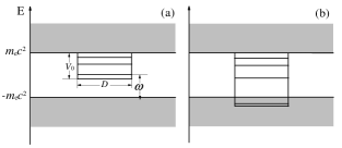
Figure 1: Sketch of the bound-continuum interaction in a binding potential well for the pair production processes. Panel (a) shows the perturbative regime in which the bound states appear in the energy gap. Pair production cannot be induced solely by the binding potential well and the laser field is necessary. In the non-perturbative regime, panel (b), the bound states overlap with the negative-energy continuum. Particles can be created by tunneling of the initially occupied negative-energy states into the quasibound states. Here the laser field is unnecessary and the tunneling dynamics cannot be treated perturbatively.

IV Enhancement of pair production in the perturbative regime

In this section, we will study the pair production process in the perturbative regime. As mentioned in Sec. III, in order to trigger pair creation, we have to superimpose a laser field onto the subcritical binding potential. Here we choose a laser field represented by the vector potential $\boldsymbol{A}(\boldsymbol{r},t)=(0,A_{0}f(t)\sin\omega(t-x/c),0)$, where $A_{0}$ is the amplitude of the potential and $\omega$ is the frequency. The time-dependent envelope $f(t)$ is the same as in Eq. (14) to characterize the turn-on and turn-off of the field.

It is well-known that the criterion for pair production is the energy provided by the external field should be at least equal or larger than the rest energy of the created particles. In our case, it means that the binding energy of the bound state and the energy of the absorbed laser photons should together be larger than $2m_{\mathrm{e}}c^{2}$. To study the effect of the locality of the bound states in the production process, we have chosen the parameters as $V_{0}=1.726m_{\mathrm{e}}c^{2}$ and $D=3.200\lambda_{c}$ as well as $V_{0}=1.900m_{\mathrm{e}}c^{2}$ and $D=2.443\lambda_{c}$, so that the energies of the ground states in both potential wells are the same $E_{\mathrm{g}}=-0.4m_{\mathrm{e}}c^{2}$. Here $\lambda_{c}$ denotes the Compton wave length for the electron. The frequency of the laser is $\omega=0.45m_{\mathrm{e}}c^{2}$, which means that the energy of the laser photon is $0.45m_{\mathrm{e}}c^{2}$, and the amplitudes $A_{0}$ is chosen such that the electric field is $E_{0}=A_{0}\omega/c=0.3E_{\mathrm{cr}}$. Since the electric field for these parameters is much smaller than the critical field, the non-perturbatively tunneling pair creation is suppressed and electrons can only be transmitted perturbatively into the ground state by absorbing two or more photons from the laser.

Since the external field used here cannot couple different spin states, we have considered only a certain spin direction (along $+z$ direction) in the simulations. Panel (a) in Fig. 2 shows the particle number $N(T)$ in the two potential wells as a function of the interaction time $T$. As most of the created electrons occupy the ground state, the average particle number should, at the end of the interaction, reach unity because of the Pauli exclusive principle. The figure, however, shows that the particle number finally exceeds unity and tends to increase linearly. This long time linear increase is a bit surprising since the bound-continuum interactions cannot induce a permanent pair creation.

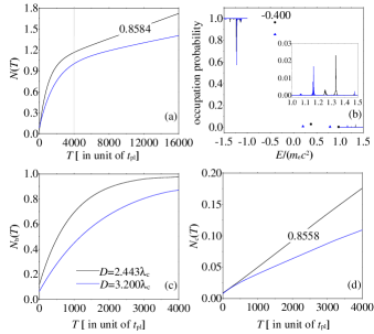
Figure 2: Figures for the pair production process in two different binding potential wells. Panel (a) is the average particle number $N(T)$ as a function of interaction time $T$. Here $t_{\mathrm{pl}}=\lambda_{c}/c$ denotes the typical time scale for the pair production process. Panel (b) is the probability of the occupation of the instantaneous state at $T=480\pi/\omega=3349t_{\mathrm{pl}}$. Panel (c) and (d) are the average particle number in the instantaneous ground state and positive continuum, respectively, as a function of time $T$. The color is coded as blue for the potential with $V_{0}=1.726m_{\mathrm{e}}c^{2}$ and $D=3.200\lambda_{c}$ and black for $V_{0}=1.900m_{\mathrm{e}}c^{2}$ and $D=2.443\lambda_{c}$. The other parameters are $W=0.3\lambda_{c}$for the potential wells and $\omega=0.45m_{\mathrm{e}}c^{2}$ and $E_{0}=A_{0}\omega/c=0.3E_{\mathrm{cr}}$ for the laser field.

To understand this linear creation and also prove our assumption that the created particles should mainly occupy the ground state in the potential well, we have, in Panel (b) of Fig. 2, displayed the occupation probability of the instantaneous states after the creation. Here the instantaneous states denote the eigenstates of the Hamiltonian of Eq. (2) with only the binding potential as the background field. The details of the method can be found in Ref. Liu et al. (2014). The almost $100\%$ occupation of the negative-energy continuum is consistent with that the vacuum state means all the negative-energy states being occupied. This is because the potential well here is subcritical and the structure of the vacuum state with or without the background potential well is similar.

Two aspects of the graph deserve further attention. First of all, despite most of the negative-energy states being fully occupied, there is a large peak in the negative continuum showing that these particular states are much less occupied. The position of this peak is around $-1.23m_{\mathrm{e}}c^{2}$ for both cases. These depopulated states are caused by the two-photon transition of the Dirac sea states into the ground state. This peak also consists with the energy of the created positrons shown below.

Secondly, the most occupied bound state in the energy gap is the ground states in both cases with energy $E_{\mathrm{g}}=-0.4m_{\mathrm{e}}c^{2}$ and all the occupation of the other bound states is negligible. This proves our conjecture that the production, in the earlier time domain, is dominated by the created electrons occupied the ground state in the potential well. What is more interesting is that there are also peaks in the positive continuum. These small peaks, which will increase with time, may be the reason of the linear increase in the particle number $N(T)$ (Panel (a)) for long interaction time.

In order to test this hypothesis, we have in Panel (c) and (d) of Fig. 2 shown the average particle number $N_{b}(T)$ occupied the instantaneous ground state $\psi^{-}(\boldsymbol{r})$ and the average particle number $N_{c}(T)$ in the positive continuum, respectively. From the graphs we can see that the population of the bound states tends to $1$ at the end while the population of the positive continuum is linearly growing in time. The sum of $N_{b}(T)$ and $N_{c}(T)$ in Panel (c) and (d) approximately equals to the total average particle number in Panel (a). More important, the linearly growing rates of $N_{c}(T)$ in Panel (d) match the slop of the total $N(T)$ curves in long interaction time $T$. For instance, the slop of the black curve in Panel (d) is about $0.8558$, which differs less than $1\%$ with the slop ($0.8584$) of the black curve in Panel (a) for long interaction time.

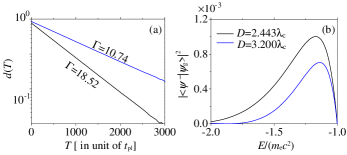
Figure 3: Decay probability $d(T)$ as a function of the interaction time $T$ is shown in Panel (a) on a logarithmic scale. The decay rate for the blue line is $\Gamma=10.74$ while for the black one is $\Gamma=18.52$. The projection of the ground state in the binding potential well onto the field-free negative energy states is shown in Panel (b). Here the ground state $\psi_{\mathrm{g}}(\boldsymbol{r})$ is the lowest energy eigenstate in the energy gap of the Hamiltonian of Eq. (2) with only the binding potential as the background field and the field-free negative continuum is $\psi^{-}(\boldsymbol{r})$. The parameters are the same as in Fig. 2.

In the early stage of the production, the process is dominated by the creation of particles in the ground state and from Fig. 2(c) it is obvious that the particle number in the ground state reaches unity at different speeds. The black curve, which is for potential well with $V_{0}=1.900m_{\mathrm{e}}c^{2}$ and $D=2.443\lambda_{c}$, has a larger speed than the blue one.

To provide a more quantitative analysis, we define $d(T)$ as

$$d(T)=|1-N_{b}(T)|\,.$$ (15)

It characterizes how fast the initial vacuum state decays into electron-positron pairs in the external fields through the ground state. Fig. 3(a) shows the quantity $d(T)$ for the two different cases on a logarithmic scale. The two straight lines indicate that the decay process is exponential, namely $d(T)\propto\exp(-\Gamma T)$ with the exponential parameter $\Gamma$ called the decay rate.

The vacuum decays much faster ($\Gamma=18.52$) in the more localized system with $D=2.443\lambda_{c}$. This is rather unexpected as it is commonly believed that the wider the state in position space, the larger the interaction region and thus the greater the possibility. In order to understand this counter-intuitive phenomenon, we have to analyze the properties of the bound states in the two potential wells.

The bound states acting like a bridge in the energy gap can help to induce pair production in this perturbative regime. Even it is not directly related to the creation rate, the nonzero overlap probability between the bound states and the field-free negative-energy states in the Dirac sea (shown in Fig. 3(b)) could still help us understand the process more intuitively. When the overlap is large, the originally occupied field free Dirac sea states would be easier to transmit into the bound state in the presence of the laser field, see also the calculations using time-dependent perturbation theory in Jiang et al. (2013). From the figure, it is clear that the more localized bound state (in the potential well of $V_{0}=1.900m_{\mathrm{e}}c^{2}$ and $D=2.443\lambda_{c}$) has a larger overlap with the negative-energy continuum. This is consistent with the larger decay rate of $\Gamma=18.52$ for the black line in Fig. 3(a).

Please note also that the long time linear creation rate shown in Fig. 2(a) has similar behavior as the decay rate $\Gamma$ of the vacuum through the bound states for short interaction time. This means that the more localized system with $D=2.443\lambda_{c}$ creates particles faster in all interaction time region.

All the simulations above are for the case that only ground state is excited in the interaction as the laser frequency is optimized for this transition only. If we want to excite other bound states, we have to either vary laser frequency or tune the potential well to make the energy difference between ground state and other bound state resonant with this laser frequency. In this circumstance, the other bound state can be excited even before the particle in the ground state saturates.

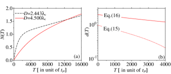
Figure 4: Particle number $N(T)$ and Decay probability $d(T)$ as a function of the interaction time $T$ for the case of two bound states involved in the pair creation is shown in Panel (a) and (b), respectively. For comparison, the dash-dot line in Panel (a) is the replot of the black curve in Fig. 2(a). In Panel (b), the decay probability with both definitions in Eq. (16) (solid) and Eq. (15) (dotted) is shown. The parameters for the potential well are $V_{0}=1.584m_{\mathrm{e}}c^{2}$ and $D=4.500\lambda_{c}$ and the laser field are the same as before.

In Fig. 4, we show the creation for such a case by change the potential well to ensure the energy difference between ground state and first excited state $\triangle E\approx\omega$. From Fig. 4(a), we see that there is no linear increase before the particle number approaching $2$. This is quite different compared with the $N(T)$ curve in Fig. 2(a). For comparison we have replotted the black curve of Fig. 2(a) as dash-dot line here. Since two bound states are excited here, the particle number will saturate at $2$ and if we want to define a decay rate as in Fig. 3(a), the definition of $d(T)$ has to be modified like

$$d(T)=|2-N(T)|\,.$$ (16)

The definition in Eq. (15) is not suitable as shown in Panel(b) of Fig. 4, where the dotted line is not a linear behavior in the logarithmic scale plot. However, the modified $d(T)$, as expected, recovers the decay processes with the rate $\Gamma=2.259$.

In this situation, the influence of the bound state’s extension on pair creation is more complicated since two bound states are excited. To concentrate on the fundamental mechanism and keep the discussion simple, we will in the following discussions still focus on the creation only involving the ground state.

Our previous results indicate that the pair creation rate decays with the extension of the bound state. This is also illustrated in Fig. 5, where the rate $\Gamma$ is shown as a function of the width $W_{\mathrm{b}}$ of the ground state. Here the width of the ground state is defined as $W_{\mathrm{b}}=2\sqrt{\langle x^{2}-\langle x\rangle^{2}\rangle}$ with $\langle x\rangle=\bra{\psi_{\mathrm{b}}(\boldsymbol{r})}\hat{x}\ket{\psi_{\mathrm{b}}(\boldsymbol{r})}$.

The decay rate shown in Fig. 5 is exponentially decaying with increasing width of the ground state, $\Gamma\propto\exp(-CW_{\mathrm{b}})$, with the constant $C$ depending on the parameters of the potential well. There are several points in the region of $2.062\lambda_{c}<W_{\mathrm{b}}<2.197\lambda_{c}$ in the figure that are not close to the normal decay trend. The reason is that the laser field in these cases happens to be able to cause resonance transitions between the bound states in the energy gap as shown in Fig. 4. Because of these resonance transitions, the population in the ground state will oscillate in time and the decay rate through this state is not as well defined as for other parameters.

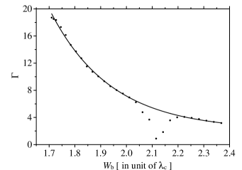
Figure 5: The decay rate $\Gamma$ as a function of the ground state width $W_{b}$. For comparison, we have chosen the parameters such that the energy of the ground states is unchanged $E_{\mathrm{g}}=-0.4m_{\mathrm{e}}c^{2}$ for different width of the states. The laser field is the same as in Fig. 2.

To complete our understanding of the decay process of the vacuum into electron-positron pairs through the bound-continuum interactions in perturbative regime, we also investigate the properties of the created positrons in momentum space. Unlike the electrons being captured in the binding potential, the created positrons are free and the momentum is sharply distributed. The distribution of the positron in momentum space $\chi^{+}(p)$ can be calculated using Eq. (10) by replacing the creation and annihilation operators for electrons to the operators for positrons. From Fig. 6, we can see that the two main peaks are around $p=\pm 0.71m_{\mathrm{e}}c$. These peaks, if we transfer to energy domain, corresponds to energy of $1.225m_{\mathrm{e}}c^{2}$, which related to the depopulated states in the negative-energy continuum in Fig. 2(b) around $E=-1.23m_{\mathrm{e}}c^{2}$. The small peaks reflect the acceleration of the positrons in the laser field after the creation. Since the laser propagates along a certain direction, the momentum distribution of the positron is not symmetric.

V Enhancement of pair production in the non-perturbative regime

In the previous sections, we studied the pair creation in the perturbative regime. The results show that the creation can be enhanced with utilization of a more localized bound state in the interactions. In order to complete the picture, we also studied the production process in a non-perturbative regime in this section. Unlike in the perturbative regime, we know from Sec. III that the non-perturbative creation is caused by the diving of the bound states into the Dirac sea as shown in Fig. 1(b).

It is known that a quasibound state, a bound state embedded in the negative continuum, can trigger the decay of the vacuum and thus produce particle pairs. Since the quasibound state is not spatially localized in the continuum, it is not clear if the locality of the true bound state before diving into the continuum still affects the pair production. As the creation is caused by the tunneling of the Dirac sea states into the initially unoccupied quasibound state, the perturbative laser field is not necessary here.

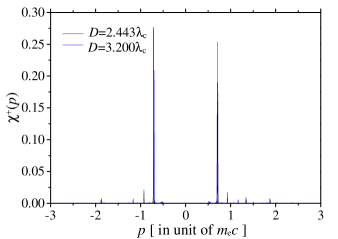
Figure 6: The momentum density of the created positrons at $T=400\pi/\omega=2791t_{\mathrm{pl}}$. Because of the field configuration we use, the only non-conserved momentum during the evolution is $p=p_{\mathrm{x}}$. For simplicity, we choose here $p_{\mathrm{y}}=p_{\mathrm{z}}=0$. The color code and the other parameters are the same as in Fig. 2.

In Fig. 7(a), we show the average particle number $N(T)$ for two supercritical potential wells with $V_{0}=2.383m_{\mathrm{e}}c^{2}$ and $V_{0}=2.522m_{\mathrm{e}}c^{2}$, respectively. For these two cases, the quasibound states are both located at $E_{\mathrm{qb}}=-1.1m_{\mathrm{e}}c^{2}$. The graph shows that $N(T)$ tends to one for $T\to\infty$ in contrast to the perturbative case in Fig. 2(a). This is because that the electron-positron pairs can only be created through the quasibound state here. With one quasibound state, the particle number can only tend to one eventually. It is obvious that the particle number tends to $1$ with different speeds. To be more quantitative, we also plot $d(T)$ as defined in Eq. (15) in Fig. 7(b). The two curves in Panel (b) of Fig. 7 indicate that the initial vacuum state also exponentially decays into electron-positron pairs through the quasibound state and the potential with $D=3.200\lambda_{c}$ triggers the faster decay. This is consistent with what happens in the perturbative regime, for example like in Fig. 3(a).

We know from the previous section that the reason for the locality-enhancement is that the more localized bound states have more overlap with the negative continuum. For the sake of verifying this explanation in the non-perturbative regime, the energy spectrum $S^{+}(E)$ of the created positrons is displayed in Fig. 7(c), which reflects the overlap between the quasibound state and the Dirac sea states. $S^{+}(E)$ is calculated by transferring the momentum distribution $\chi^{+}(p)$ to the energy domain. The two spectra have the similar location for the maximum value, which corresponds to the energy of the quasibound states. However, the spectrum for the case of $D=3.200\lambda_{c}$ is much wider than that for $D=4.000\lambda_{c}$. This means that the quasibound state in the narrower potential well, even it is not spatially localized, has a larger overlap with the negative continuum. On the other hand, the full width at half maximum of the two spectra are consistent with the decay rate in Fig. 7(b).

It is also worth pointing out that the enhancement in this non-perturbative creation regime might be seen in connection with the well-known non-Markovian feature of the pair production process Schmidt et al. (1998, 1999), as the quasibound state inherits some properties from its original bound state. Because the ground state in the potential well with $D=3.200\lambda_{c}$ is more localized in the energy gap, its narrow distribution in position space still amplifies the creation process even after it dives into the negative Dirac sea and becomes the unlocalized quasibound state.

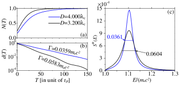
Figure 7: The average particle number $N(T)$ and the decay probability $d(T)$ as a function of the interaction time $T$ is plotted, respectively, in Panel (a) and (b). The decay probability $d(T)$ is shown in logarithmic scale. The energy spectrum $S^{+}(E)$ of the created positron for $T=282t_{\mathrm{pl}}$ is shown in Panel (c). The parameters for the blue curves are $V_{0}=2.383m_{\mathrm{e}}c^{2}$ and $D=4.000\lambda_{c}$ and for the black curves are $V_{0}=2.522m_{\mathrm{e}}c^{2}$ and $D=3.200\lambda_{c}$. The quasibound states in both potential wells have the energy $E_{\mathrm{qb}}=-1.1m_{\mathrm{e}}c^{2}$. The choice of the parameters insures that the bound states in these two potential well have different spatial widths before diving into the negative continuum.

VI Summary and outlook

The purpose of this work is to study the influence of the locality of a bound state in the pair production process. The feasibility of this work is the CQFT method, which can give us the full space-time resolution of the pair production process in any general external field. By analyzing the average particle number, we can clearly see the enhancement of the pair creation process caused by a more localized bound state. Even with the same binding energy, the vacuum will decay faster through the bound state with narrower distribution in position space. This also means that energy threshold is not the only criterion for pair creation as some other properties of the bound states can play a role in the bound-continuum interaction induced pair production.

The enhancement manifest itself in both perturbative and non-perturbative regimes, which intrinsically have completely different mechanisms for triggering pair creation. In the perturbative regime, the electron-positron pairs are created by multi-photon excitation as seen from the momentum spectrum of the created positrons. The bound states act like an intermediary in the process, which makes it also easier to understand that the properties of the bound states play an important role in the production. In the non-perturbative regime, on the other hand, the electron-positron pairs are created by the tunneling of the initially occupied Dirac sea states into the quasibound states, which are not localized in space at all. The properties of the bound states before diving into the negative continuum and becoming the quasibound state, however, still influence the pair creation processes. This can be viewed as the non-Markovian feature Schmidt et al. (1998, 1999) of the production.

This enhancement may be detected in the laboratory using the Bethe-Heitler process Augustin and Müller (2014); Lötstedt et al. (2008), interacting a strong laser pulse with a highly charged ion or a nucleus. Because of the screen effect in a highly charged ion, a nucleus with similar charge as an ion, based on our results, will produce more electron-positron pairs when interacting with the same laser pulse. On the other hand, pair creation here is triggered by bound states in a binding potential well. Whereas in a strong magnetic field, the energy spectrum of the system will also be discretized Landau and Lifshitz (1981). The creation processes under this field configuration might be amplified by these Landau levels. Likewise, the spin of the created electrons and positrons might play a role under magnetic field. Because of this internal degree of freedom the enhancement effect may appear in different manifestations, but much more systematic studies to test these conjectures are necessary. We will report on these in future works.