Existence of a Spectral Gap in the Affleck-Kennedy-Lieb-Tasaki Model on the Hexagonal Lattice

Abstract

The $S=1$ Affleck-Kennedy-Lieb-Tasaki (AKLT) quantum spin chain was the first rigorous example of an isotropic spin system in the Haldane phase. The conjecture that the $S=3/2$ AKLT model on the hexagonal lattice is also in a gapped phase has remained open, despite being a fundamental problem of ongoing relevance to condensed-matter physics and quantum information theory. Here we confirm this conjecture by demonstrating the size-independent lower bound $\Delta>0.006$ on the spectral gap of the hexagonal model with periodic boundary conditions in the thermodynamic limit. Our approach consists of two steps combining mathematical physics and high-precision computational physics. We first prove a mathematical finite-size criterion which gives an analytical, size-independent bound on the spectral gap if the gap of a particular cut-out subsystem of 36 spins exceeds a certain threshold value. Then we verify the finite-size criterion numerically by performing state-of-the-art DMRG calculations on the subsystem.

The manifestations of antiferromagnetism in quantum spin systems depend sensitively on the underlying geometry and spin number. A subtle and famous instance of this connection was proposed by Haldane, who predicted in 1983 that the Heisenberg spin chain has a spectral gap above the ground state whenever the spin $S$ per site is an integer H83a ; H83b . Motivated by his considerations, Affleck, Kennedy, Lieb, and Tasaki (AKLT) introduced a new family of quantum spin systems in 1987 and proved that their one-dimensional $S=1$ version is indeed in Haldane’s eponymous quantum phase AKLT87 ; AKLT88 . The influence of the seminal AKLT papers continues to this day: the valence-bond solid (VBS) aspect of the AKLT construction directly inspired the development of concepts that are by now central tenets of modern quantum physics, such as matrix product states, projected entangled pair states (PEPS), and more generally tensor network states Cetal1 ; Cetal2 ; FNW ; O14 ; S11 ; Schuchetal1 ; Schuchetal2 . Moreover, the non-local string order exhibited by the AKLT chain KT ; NR ; Pollmannetal has been developed much further into the more general concept of symmetry-protected topological order Chenetal ; FK ; Morimotoetal ; Nussinov . Finally, the AKLT ground states on some two-dimensional lattices, including the $S=3/2$ model on the hexagonal lattice, provide rare instances of a universal resource state for measurement-based quantum computation (MBQC) VC ; WAR11 ; WHR14 ; M .

One of the main accomplishments of the original AKLT works AKLT87 ; AKLT88 is the rigorous derivation of a spectral gap above the AKLT ground state in one dimension. AKLT also investigated the $S=3/2$ model on the hexagonal lattice and were able to demonstrate the exponential decay of the spin-spin correlations for the exact VBS ground state with periodic boundary conditions, and on the basis of this fact they conjectured that the hexagonal model also exhibits a spectral gap (see also KLT88 ). We recall that a spectral gap implies the decay of ground state correlations, but not vice-versa Fernandezetal1 ; Fernandezetal2 ; HK ; N ; NS . Evidence pointing to a spectral gap has been mounting Aetal ; DB16 ; GMW ; KLT88 ; K ; LSY ; PW19 , but, despite the paradigmatic role played by the hexagonal AKLT model, the long-standing fundamental problem to show that its spectrum is gapped has remained unresolved. The presence of a gap would have broader consequences, e.g., in supporting the widespread heuristic that PEPS arise from gapped Hamiltonians, see the recent review Ciracetal , and for the complexity and stability of the corresponding universal resource states for MBQC VC ; WAR11 ; WHR14 ; M . One of the main reasons why the AKLT conjecture has remained unresolved is that, while the ground states of the hexagonal AKLT model can be written down exactly, only very little is known about its excited states. More generally, the existing mathematical techniques for deriving spectral gaps in quantum spin systems of dimensions $\geq 2$ are quite limited. The few examples where a spectral gap is known to exist include the product vacua with boundary states (PVBS) models BHNY ; B ; LN and, since recently, decorated variants of the AKLT models Aetal ; PW19 .

Figure 1: The patch $\Lambda_{m_{1},m_{2}}$ with parameters $m_{1}=6$ and $m_{2}=4$. ($m_{1}$ and $m_{2}$ are the width and height of $\Lambda_{m_{1},m_{2}}$ in units of hexagonal cells, respectively.) Periodic oundary conditions are imposed by identifying the boundary vertices which are assigned the same letter. Note that the letters A and B appear three times in total.

In this Letter, we confirm the AKLT conjecture by demonstrating a lower bound, $\Delta>0.006$, on the spectral gap of the hexagonal model. More precisely, we consider a sequence of AKLT models where the hexagonal lattice is wrapped on an $m_{1}\times m_{2}$ torus and show that their spectral gaps are all bounded from below by $0.006$ for arbitrarily large system-size parameters $m_{1}$ and $m_{2}$; see Fig. 1 for the definition of the periodic boundary conditions on a $6\times 4$ torus. Methodologically, our approach consists of two steps. Step 1 comes from mathematical physics and step 2 is based on state-of-the-art computational physics. In step 1, we prove a mathematical finite-size criterion which is tailor-made for the problem at hand. In a nutshell, the finite-size criterion says that, if the spectral gap of the $36$-site cluster displayed in Fig. 2 exceeds an explicit numerical threshold, then the AKLT model has a spectral gap for all system sizes $m_{1},m_{2}$. To prove the criterion, we follow the combinatorial approach pioneered by Knabe K , strengthened by using interaction weights as in Refs. GM ; LM . In step 2, we combine the rigorous analytical insight from step 1 by numerically verifying the finite-size criterion via a high-precision density-matrix renormalization group (DMRG) calculation (see also Ref. LSY for a one-dimensional analog studied with Lanczos diagonalization). We present tests of the correctness of our implementation of the well-established DMRG method in the Supplemental Material (SM) [40]. Since it is not possible to establish a rigorous precise estimate of any remaining convergence errors, our result may not be considered a rigorous mathematical proof as a matter of principle. However, in practice, the computed gap exceeds the threshold by such a wide margin that it can be regarded as a conclusive demonstration.

One challenge in the numerical part of the argument is that the relevant open-boundary system (Fig. 2), whose gap we need to compute, has a massive ground state degeneracy due to the 12 “dangling” effective boundary $S=1$ spins which arise in the AKLT construction when only one out of the three nearest-neighbor couplings is active. This results in a $3^{12}$-fold ground state degeneracy. To reduce the number of levels which has to be converged, we use a variant of DMRG with full $\mathrm{SU}(2)$ symmetry and calculate the ground state and several excited states over all sectors of total spin. Crucially, in the process of successively orthogonalizing the calculations to previously converged states, we have used the AKLT construction to exactly project out the full degenerate subspace. Without this preliminary step, which we discuss further below and describe in more detail in SM , it would currently not be possible to converge the excited states in all total spin ($J$) sectors and conclusively identify the smallest gap of the system. We find that the lowest gap originates from the $J=13$ sector and that it exceeds the analytical gap threshold well beyond any conceivable remaining DMRG truncation errors.

Our main result is a size-independent lower bound on the spectral gap of the AKLT Hamiltonian on finite patches of the hexagonal lattice $\mathbb{H}$ with periodic boundary conditions, which we call $\Lambda_{m_{1},m_{2}}$. The key point is that the lower bound on the gap is independent of the size parameters $m_{1}$ and $m_{2}$ of these patches and thus extends to the thermodynamic limit.

For $m_{1}$ and $m_{2}$ two positive integers, the finite patch $\Lambda_{m_{1},m_{2}}$ is defined by wrapping the hexagonal lattice on an $m_{1}\times m_{2}$ torus. We invite the reader to view Fig. 1 for a specific example of how the periodic boundary conditions are realized.

Figure 2: The fixed-size patch $\mathcal{F}$ whose spectral gap we compute numerically. It is equipped with open boundary conditions, in contrast to $\Lambda_{m_{1},m2}$. The weights $w_{e}$ in Eq. (5) are assigned as follows: Dashed edges are weighted by $w_{e}=a\geq 1$ as indicated, while all other edges are unweighted (i.e., $w_{e}=1$).

Since the hexagonal lattice has valence $3$, one takes each site to host an $S=3/2$ spin and considers the Hilbert space

$$\mathcal{H}_{m_{1},m_{2}}=\bigotimes_{j\in\Lambda_{m_{1},m_{2}}}\mathbb{C}^{4}.$$ (1)

On $\mathcal{H}_{m_{1},m_{2}}$, the AKLT Hamiltonian is defined by

$$H^{AKLT}_{m_{1},m_{2}}=\sum_{\begin{subarray}{c}j,k\in\Lambda_{m_{1},m_{2}}:\\ j\sim k\end{subarray}}P_{j,k}^{(3)},$$ (2)

where $P_{j,k}^{(3)}$ denotes the projection onto total spin $3$ across the bond connecting vertices $j$ and $k$. By convention, the neighboring relation $\sim$ includes the periodic boundary conditions inherent to $\Lambda_{m_{1},m_{2}}$.

As a sum of projections, the Hamiltonian $H^{AKLT}_{m_{1},m_{2}}$ is automatically a positive semidefinite operator. The valence-bond construction of AKLT AKLT87 ; AKLT88 yields a ground state which is a non-zero element of $\ker H^{AKLT}_{m_{1},m_{2}}$, making this Hamiltonian frustration-free. Its spectral gap $\gamma^{AKLT}_{m_{1},m_{2}}$ is the smallest strictly positive eigenvalue, that is,

$$\gamma^{AKLT}_{m_{1},m_{2}}=\inf\mathrm{spec}\left(H^{AKLT}_{m_{1},m_{2}}\right)\setminus\{0\}.$$ (3)

We can now state our main result, which provides a lower bound on the spectral gap $\gamma^{AKLT}_{m_{1},m_{2}}$ that is independent of the system size parameters $m_{1}$ and $m_{2}$.

Main result. Let $m_{1},m_{2}\geq 12$. Then, it holds that

$$\gamma^{AKLT}_{m_{1},m_{2}}\geq 0.00646.$$ (4)

A few remarks about this result are in order: (i) We work with periodic boundary conditions for convenience and the results imply a bulk gap in the thermodynamic limit under these boundary conditions. Moreover, it was proved in Ref. KLT88 that the infinite-volume ground state is unique. (ii) This main result is not a rigorous mathematical theorem because it relies on numerical input from the DMRG algorithm. While the DMRG algorithm becomes exact for large bond dimension and the computations are sufficiently precise and well-tested to firmly establish (4) beyond doubt, we do not claim to have a mathematical proof of sufficiently tight error estimates. (iii) From previous numerical investigations, see e.g. GMW , it is believed that the true spectral gap of the hexagonal model is $\approx 0.1$, but the results depend on extrapolations in the system size that assume that an asymptotic scaling regime has been reached.

The finite-size criterion.—We now discuss the main mathematical tool, which is a finite-size criterion for deriving a spectral gap. In a nutshell, it says that if the spectral gap of the system $\mathcal{F}$ depicted in Fig. 2 exceeds some explicit numerical threshold, then we also obtain a lower bound on the spectral gap $\gamma_{m_{1},m_{2}}^{AKLT}$ that is independent of the size parameters $m_{1},m_{2}$ as desired. The intuition behind the finite-size criterion is that, thanks to the frustration-freeness of the AKLT Hamiltonian, the problem of finding the lowest possible excitation energy (gap) is a local question. Hence, it is enough to know that local patches of the whole system are “sufficiently gapped” in a way that the criterion makes precise. For related finite-size criteria that ours here is inspired by, see Refs. K ; GM ; LM ; L1 ; Anshu ; L2 ; LSY . The idea behind the finite-size criterion is to construct $H_{m_{1},m_{2}}^{AKLT}$ from translated copies of an appropriate finite-size Hamiltonian, which we call $H_{\mathcal{F}}$. For the criterion to work in practice, the patch has to be sufficiently large because the criterion depends on the cluster size and shape, and even if there is a gap in the thermodynamic limit the finite-size criterion may not be satisfied on a small cluster. Our criterion is based on the following Hamiltonian $H_{\mathcal{F}}$ defined on the 36-site patch $\mathcal{F}$ shown in Fig. 2, with open boundary conditions.

The patch lives on the local Hilbert space $\mathcal{H}_{\mathcal{F}}=\bigotimes_{j\in\mathcal{F}}\mathbb{C}^{4}.$ We write $\mathcal{E}_{\mathcal{F}}$ for the set of edges $e=(j,k)$ with $j,k\in\mathcal{F}$, i.e., we equip $\mathcal{F}$ with open boundary conditions (in contrast to $\Lambda_{m_{1},m_{2}}$). Let $a\geq 1$ be a parameter. We define the finite-size Hamiltonian by

$$H_{\mathcal{F}}=\sum_{e\in\mathcal{E}_{\mathcal{F}}}w_{e}P_{e}^{(3)},$$ (5)

where $P_{e}^{(3)}$ is the projection onto total spin $3$ for the pair of vertices $j,k$ that form the endpoints of the edge $e$. The weights $w_{e}$ are defined as follows:

$$w_{e}=\begin{cases}a,&\textnormal{if the edge $e$ is labeled by $a$ in Fig.\leavevmode\nobreak\ \ref{fig:F}},\\ 1,&\textnormal{otherwise}.\end{cases}$$ (6)

The valence-bond ground state construction of AKLT AKLT87 ; AKLT88 still applies to $H_{\mathcal{F}}$ and proves that it is frustration-free. Its spectral gap is $\gamma_{\mathcal{F}}(a)=\inf\mathrm{spec}\left(H_{\mathcal{F}}\right)\setminus\{0\}.$

Theorem (The finite-size criterion).

Let $m_{1},m_{2}\geq 12$ be integers and let $a\geq 1$. Then we have the gap bound

$$\gamma^{AKLT}_{m_{1},m_{2}}\geq\frac{10+4a}{3a^{2}+2a+7}\left(\gamma_{\mathcal{F}}(a)-\frac{a^{2}-2a+3}{10+4a}\right).$$ (7)

The general way of applying this theorem goes as follows: If for some parameter value $a\geq 1$, one finds that the finite–size gap $\gamma_{\mathcal{F}}(a)$ exceeds the threshold $\frac{a^{2}-2a+3}{10+4a}$, then (7) provides a lower bound on $\gamma^{AKLT}_{m_{1},m_{2}}$ that is independent of $m_{1},m_{2}$ (subject to $m_{1},m_{2}\geq 12$ of course). The proof of the finite-size criterion is deferred to the SM SM .

We now follow this procedure to show the spectral gap bound (4). As explained in detail further below, by a numerical DMRG calculation we obtain the following explicit lower bound on the finite-size gap $\gamma_{\mathcal{F}}(a)$ with $a=1.4$,

$$\gamma_{\mathcal{F}}(1.4)>0.145.$$ (8)

This value exceeds the gap threshold $\frac{a^{2}-2a+3}{10+4a}\approx 0.138$, and thus verifies the finite-size criterion. The exact numerical bound on $\gamma^{AKLT}_{m_{1},m_{2}}$ can be computed by noting that $\frac{a^{2}-2a+3}{10+4a}<0.1385$ and $\frac{10+4a}{3a^{2}+2a+7}>0.994$, which together with (8) can be applied to (7) to show

$$\gamma^{AKLT}_{m_{1},m_{2}}\geq 0.994\left(0.145-\frac{a^{2}-2a+3}{10+4a}\right)\geq 0.00646$$

This establishes the main result, the spectral gap bound (4).

DMRG calculations.—We next discuss our implementation of the DMRG algorithm and results for the gap of the open boundary 36-site cluster $\mathcal{F}$ shown in Fig. 2. Additional details, including detailed convergence tests, are relegated to the SM SM .

The ground states of the cluster $\mathcal{F}$ can be understood as follows: each physical $S=3/2$ spin is made out of 3 auxiliary $S=1/2$ spins, each of which will pair with another auxiliary $S=1/2$ from a neighboring site, forming a singlet and dropping out. This construction ensures that any pair of neighboring physical $S=3/2$ spins can never fuse into a total spin-$3$ state, and the AKLT ground state condition is therefore fullfilled. However on the open boundary sites, two auxiliary $S=1/2$ spins per site are left over, and these are only allowed to fuse into an $S=1$ state due to the symmetric constraint. Therefore, there are 12 boundary $S=1$ degrees of freedom that can form any total spin $0\leq J\leq 12$, spanning a degenerate ground state manifold of dimension $3^{12}$. The lowest excitation above the ground states, which can be interpreted as swapping a bulk singlet with a triplet that further fuses with the boundary total angular momentum, can in principle form any angular momentum $0\leq J\leq 13$. In order to conclusively determine the smallest nonzero gap among all possible total-spin sectors, one has to find the lowest excitation in every sector $J\in\{0,1,\ldots,13\}$. For even higher $J$ sectors, the lowest excitation requires breaking more than one singlet and therefore costs significantly more energy. For completeness we also computed the gaps in all other sectors where $J>13$.

An $\mathrm{SU}(2)$ symmetric DMRG algorithm is used to automatically generate the degenerate ground state manifold in all sectors of total spin $J\in\{0,1,\ldots,12\}$ and compute the lowest excited state therein by projecting out the complete ground state manifold exactly. Two of us previously used such an orthogonalization procedure for successively converging excited states of a different model prl121.107202 , but here the simple form of the degenerate AKLT ground-state manifold enables us to eliminate it directly. Let $L$ denote the maximum-spin multiplet formed by the unpaired boundary $S=1$ spins in the ground state manifold. For the 36-site cluster in Fig. 2 we have $L=12$. The ground state manifold contains the following number of states with total spin $J$: 4213 ($J=0$), 11298 ($J=1$), 15026 ($J=2$), 14938 ($J=3$), 12078 ($J=4$), 8162 ($J=5$), 4642 ($J=6$), 2211 ($J=7$), 869 ($J=8$), 274 ($J=9$), 66 ($J=10$), 11 ($J=11$), and 1 ($J=12$). Accordingly, the lowest excitation for each $J$ is computed by projecting out that many degenerate ground states, which make the excited state computationally challenging. For sectors with total spin $J>L$, which are devoid of ground states, the lowest excitation can be computed more straight-forwardly without projecting out any states. Upon computing the lowest excitation gaps for all $J\leq L+1$ sectors of the 36-site cluster at $a=1.4$, we found that the smallest one originates from the $J=L+1=13$ sector; in Fig. 3 we show results for $J=11,12$, and $13$. The $J=13$ gap obtained by extrapolating to vanishing DMRG discarded weight $\epsilon$ is $\Delta(13)=0.14599$. The lowest gaps within all other $J$ sectors remain well above $\Delta(13)$ and there is no doubt (but also no rigorous proof) that the smallest gap exceeds the relevant threshold $0.138$. In the SM, the convergence of the gaps with $\epsilon$ is illustrated in Fig. S8 for all $0\leq J\leq 16$.

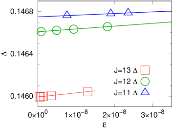
Figure 3: Gaps in the sectors $J=11,12$, and $13$ graphed versus the DMRG discarded weight $\epsilon$. The discarded weight decreases with increasing number of $\mathrm{SU}(2)$ states used, and we used up to $D=2400$ for $J=11,12$, and up to $D=1200$ for $J=13$. Line fits are used for $\epsilon\to 0$ extrapolation.

Conclusions.—We have verified the AKLT conjecture from 1987 that the hexagonal AKLT model has a spectral gap above the ground state. This confirms that the original Hamiltonian with a PEPS ground state is gapped, a question emphasized, e.g., in the recent collection of open problems Ciracetal . More generally, the existence of a spectral gap is an immensely consequential property in any quantum many-body system. First, a spectral gap implies the exponential decay of ground state correlations (but not vice-versa) Fernandezetal1 ; Fernandezetal2 ; HK ; N ; NS and is expected to imply other complexity bounds on the ground state such as the area law for the entanglement entropy. Second, the existence of a spectral gap is a crucial assumption in the classification of topological quantum phases and the many-body adiabatic theorem BBDF ; BDRF ; BMNS12 ; BHM10 ; H04 ; HW . We also mention that the existence of a spectral gap is perturbatively stable BHM10 ; H19 ; dRS ; FP ; MZ . While our result confirms the long-standing AKLT conjecture, we hope that it inspires future work on the spectral gap of this timeless model. In particular, we believe that it would be useful to have a purely analytical derivation of a spectral gap, because the argument here relies on numerical computations without suitable rigorous error bounds and because a purely analytical argument will presumably be accompanied by an improved understanding of the model’s low-energy excitations.

Let us briefly discuss the wider scope of the approach we use here. The mathematical physics step is the derivation of a finite-size criterion in the general spirit of Knabe’s combinatorial criteria K with weights as in Refs. GM ; LM . The computational physics step consists of verifying the finite-size criterion by a high-precision DMRG implementation. Our approach of numerically verifying a combinatorial finite-size criterion is in principle applicable to any frustration-free spin system. Concerning the AKLT models, for example, the square lattice is a natural next candidate to consider AAH ; GMW ; PW19 , as well as $\mathrm{SU}(n)$-symmetric variants GS ; WNM ; GP . The cubic lattice is another interesting case which also displays novel phase-transition phenomena PSA09 .

Note added: After our preprint appeared, Pomata and Wei PWrecent demonstrated the existence of a spectral gap in AKLT models on various two-dimensional degree-$3$ lattices including the hexagonal lattice. Their argument is different, but it also combines analytics (inspired by Aetal ; PW19 ) with numerics.

I Supplementary Material

Existence of a spectral gap in the AKLT model on the hexagonal lattice

Marius Lemm, Anders W. Sandvik, and Ling Wang

In Section I, we present the detailed proof of the finite-size criterion. In Section II, we explain details concerning the implementation of the $\mathrm{SU}(2)$ symmetric DMRG method. In Section III, we demonstrate the correctness of our method of exactly projecting out the ground state manifold on a 12-site cluster, for which the gaps can be computed exactly. We also demonstrate the convergence of the lowest gaps in all total-spin sectors $J\in\{0,1,\ldots 54\}$ of the 36-site cluster on the basis of which our conclusions on the numerical gap bound is drawn.

I.1 I. Proof of the finite-size criterion

I.2 Squaring the Hamiltonian

Fix two integers $m_{1},m_{2}\geq 12$. In the following, we abbreviate $H^{AKLT}_{m_{1},m_{2}}=H$, $P^{(3)}_{e}=P_{e}$ and $\gamma_{\mathcal{F}}(a)=\gamma_{\mathcal{F}}$.

By frustration-freeness and the spectral theorem, the claimed gap inequality (7) is equivalent to the operator inequality

$$H^{2}\geq\frac{10+4a}{3a^{2}+2a+7}\left(\gamma_{\mathcal{F}}-\frac{a^{2}-2a+3}{10+4a}\right)H.$$ (S1)

As usual, an operator inequality $A\leq B$ is defined to mean that the operator $B-A$ is positive semidefinite.

Our goal is now to prove Eq. (S1). We begin by computing $H^{2}$. Let us introduce some convenient notation. We write $\mathcal{E}_{m_{1},m_{2}}$ for the set of edges of $\Lambda_{m_{1},m_{2}}$ considered with periodic boundary conditions. Given two distinct edges $e$ and $e^{\prime}$, we write $e\sim e^{\prime}$ if $e\neq e^{\prime}$ and the edges share a vertex, and we write $e\not\sim e^{\prime}$, if $e\neq e^{\prime}$ and the edges do not share a vertex. We also introduce the notation

$$\{A,B\}=AB+BA$$

for the anticommutator of two operators $A$ and $B$.

Using that $P_{e}^{2}=P_{e}$, we have

$$H^{2}=H+Q+R,$$ (S2)

where we introduced the operators

$$Q= \sum_{\begin{subarray}{c}e,e^{\prime}\in\mathcal{E}_{m_{1},m_{2}}:\\ e\sim e^{\prime}\end{subarray}}\{P_{e},P_{e^{\prime}}\},$$ (S3)

$$R= \sum_{\begin{subarray}{c}e,e^{\prime}\in\mathcal{E}_{m_{1},m_{2}}:\\ e\not\sim e^{\prime}\end{subarray}}\{P_{e},P_{e^{\prime}}\}.$$

I.3 Shifted finite-size systems and the auxiliary operator

The idea is to construct the full Hamiltonian $H$ from translated copies of the finite-size Hamiltonian $H_{\mathcal{F}}$, viewed as subsystems acting on the common Hilbert space $\mathcal{H}_{m_{1},m_{2}}$ from (1).

Let us introduce some formal setup and notation. We write $\mathcal{P}_{m_{1},m_{2}}$ for the set of plaquettes in $\Lambda_{m_{1},m_{2}}$. Given a fixed plaquette $\leavevmode\hbox to11.04pt{\vbox to9.67pt{\text{[drawing]}}}\in\mathcal{P}_{m_{1},m_{2}}$, we write $\mathcal{F}_{\leavevmode\hbox to6.49pt{\vbox to5.73pt{\text{[drawing]}}}}$ for a copy of the patch $\mathcal{F}$ which has as its central plaquette and otherwise respects the periodic boundary conditions imposed by $\Lambda_{m_{1},m_{2}}$. The edge set $\mathcal{E}_{\mathcal{F}_{\leavevmode\hbox to6.49pt{\vbox to5.73pt{\text{[drawing]}}}}}$ is then defined accordingly, i.e., it respects the periodic boundary conditions of $\Lambda_{m_{1},m_{2}}$ and also the open boundary conditions of $\mathcal{F}_{\leavevmode\hbox to6.49pt{\vbox to5.73pt{\text{[drawing]}}}}$. (Here we use that $m_{1},m_{2}\geq 12$, so that these boundary requirements do not interfere.)

On the common Hilbert space $\mathcal{H}_{m_{1},m_{2}}$ from (1), we can then define the family of translated finite-size Hamiltonians

$$H_{\mathcal{F}_{\leavevmode\hbox to6.49pt{\vbox to5.73pt{\text{[drawing]}}}}}=\sum_{e\in\mathcal{E}_{\mathcal{F}_{\leavevmode\hbox to6.49pt{\vbox to5.73pt{\text{[drawing]}}}}}}w_{e}P_{e},\qquad\textnormal{ for every }\leavevmode\hbox to11.04pt{\vbox to9.67pt{\text{[drawing]}}}\in\mathcal{P}_{m_{1},m_{2}}.$$

We observe that these Hamiltonians are all unitarily equivalent to $H_{\mathcal{F}}$. In particular, they are frustration-free and their spectral gaps are all equal to $\gamma_{\mathcal{F}}.$

We introduce the auxiliary operator

$$\mathcal{A}=\sum_{\leavevmode\hbox to6.49pt{\vbox to5.73pt{\text{[drawing]}}}\in\mathcal{P}_{m_{1},m_{2}}}H_{\mathcal{F}_{\leavevmode\hbox to6.49pt{\vbox to5.73pt{\text{[drawing]}}}}}^{2}.$$

We have the following key lemma.

Lemma 1.

Let $m_{1},m_{2}\geq 12$ be integers and let $a\geq 1$.

We have the two operator inequalities

$$\mathcal{A}\geq (10+4a)\gamma_{\mathcal{F}}H,$$ (S4)

$$\mathcal{A}\leq (10+4a^{2})H+(3a^{2}+2a+7)(Q+R).$$ (S5)

Proof.

We first prove (S4). By frustration-freeness and the spectral theorem, it holds that

$$H_{\mathcal{F}_{\leavevmode\hbox to6.49pt{\vbox to5.73pt{\text{[drawing]}}}}}^{2}\geq\gamma_{\mathcal{F}_{\leavevmode\hbox to6.49pt{\vbox to5.73pt{\text{[drawing]}}}}}H_{\mathcal{F}_{\leavevmode\hbox to6.49pt{\vbox to5.73pt{\text{[drawing]}}}}}=\gamma_{\mathcal{F}}H_{\mathcal{F}_{\leavevmode\hbox to6.49pt{\vbox to5.73pt{\text{[drawing]}}}}}.$$

In the second step, we used that $\gamma_{\mathcal{F}_{\leavevmode\hbox to6.49pt{\vbox to5.73pt{\text{[drawing]}}}}}=\gamma_{\mathcal{F}}$ by unitary equivalence of the corresponding Hamiltonians. When we sum this operator inequality over plaquettes $\leavevmode\hbox to11.04pt{\vbox to9.67pt{\text{[drawing]}}}\in\mathcal{P}_{m_{1},m_{2}}$, we find

$$\mathcal{A}\geq\gamma_{\mathcal{F}}\sum_{\leavevmode\hbox to6.49pt{\vbox to5.73pt{\text{[drawing]}}}\in\mathcal{P}_{m_{1},m_{2}}}H_{\mathcal{F}_{\leavevmode\hbox to6.49pt{\vbox to5.73pt{\text{[drawing]}}}}}=\gamma_{\mathcal{F}}\sum_{\leavevmode\hbox to6.49pt{\vbox to5.73pt{\text{[drawing]}}}\in\mathcal{P}_{m_{1},m_{2}}}\sum_{e\in\mathcal{E}_{\mathcal{F}_{\leavevmode\hbox to6.49pt{\vbox to5.73pt{\text{[drawing]}}}}}}w_{e}P_{e}.$$ (S6)

By translation invariance, each $e\in\mathcal{E}_{m_{1},m_{2}}$ appears the same number of times in the combined summation $\sum_{\leavevmode\hbox to6.49pt{\vbox to5.73pt{\text{[drawing]}}}\in\mathcal{P}_{m_{1},m_{2}}}\sum_{e\in\mathcal{E}_{\mathcal{F}_{\leavevmode\hbox to6.49pt{\vbox to5.73pt{\text{[drawing]}}}}}}$, where we also account for the number of times the edge is accompanied by the weight factor $a$ arising from (6). In other words, the sum of local Hamiltonians $\sum_{\leavevmode\hbox to6.49pt{\vbox to5.73pt{\text{[drawing]}}}\in\mathcal{P}_{m_{1},m_{2}}}H_{\mathcal{F}_{\leavevmode\hbox to6.49pt{\vbox to5.73pt{\text{[drawing]}}}}}$ is a multiple of the full Hamiltonian $H$, where the multiplicative factor reflects the weighted number of times each edge appears in a copy of $\mathcal{F}_{\leavevmode\hbox to6.49pt{\vbox to5.73pt{\text{[drawing]}}}}$. We find that a given edge $e\in\mathcal{E}_{m_{1},m_{2}}$ appears $10$ times as an unweighted edge in a $\mathcal{F}_{\leavevmode\hbox to6.49pt{\vbox to5.73pt{\text{[drawing]}}}}$, and $4$ times as an $a$-weighted edge. These combinatorial considerations show that

$$\sum_{\leavevmode\hbox to6.49pt{\vbox to5.73pt{\text{[drawing]}}}\in\mathcal{P}_{m_{1},m_{2}}}H_{\mathcal{F}_{\leavevmode\hbox to6.49pt{\vbox to5.73pt{\text{[drawing]}}}}}=(10+4a)H,$$ (S7)

which together with (S6) proves (S4).

It remains to prove (S5). Since $P_{e}^{2}=P_{e}$, we have as in (S2),

$$H_{\mathcal{F}_{\leavevmode\hbox to6.49pt{\vbox to5.73pt{\text{[drawing]}}}}}^{2}=\tilde{H}_{\mathcal{F}_{\leavevmode\hbox to6.49pt{\vbox to5.73pt{\text{[drawing]}}}}}+Q_{\mathcal{F}_{\leavevmode\hbox to6.49pt{\vbox to5.73pt{\text{[drawing]}}}}}+R_{\mathcal{F}_{\leavevmode\hbox to6.49pt{\vbox to5.73pt{\text{[drawing]}}}}},$$

with

$$\tilde{H}_{\mathcal{F}_{\leavevmode\hbox to6.49pt{\vbox to5.73pt{\text{[drawing]}}}}}= \sum_{\begin{subarray}{c}e,e^{\prime}\in\mathcal{E}_{\mathcal{F}_{\leavevmode\hbox to6.49pt{\vbox to5.73pt{\text{[drawing]}}}}}:\\ e\sim e^{\prime}\end{subarray}}w_{e}^{2}P_{e},$$ (S8)

$$Q_{\mathcal{F}_{\leavevmode\hbox to6.49pt{\vbox to5.73pt{\text{[drawing]}}}}}= \sum_{\begin{subarray}{c}e,e^{\prime}\in\mathcal{E}_{\mathcal{F}_{\leavevmode\hbox to6.49pt{\vbox to5.73pt{\text{[drawing]}}}}}:\\ e\sim e^{\prime}\end{subarray}}w_{e}w_{e^{\prime}}\{P_{e},P_{e^{\prime}}\},$$

$$R_{\mathcal{F}_{\leavevmode\hbox to6.49pt{\vbox to5.73pt{\text{[drawing]}}}}}= \sum_{\begin{subarray}{c}e,e^{\prime}\in\mathcal{E}_{\mathcal{F}_{\leavevmode\hbox to6.49pt{\vbox to5.73pt{\text{[drawing]}}}}}:\\ e\not\sim e^{\prime}\end{subarray}}w_{e}w_{e^{\prime}}\{P_{e},P_{e^{\prime}}\}.$$

Next, we sum this identity over plaquettes $\leavevmode\hbox to11.04pt{\vbox to9.67pt{\text{[drawing]}}}\in\mathcal{P}_{m_{1},m_{2}}$,

$$\mathcal{A}=\sum_{\leavevmode\hbox to6.49pt{\vbox to5.73pt{\text{[drawing]}}}\in\mathcal{P}_{m_{1},m_{2}}}\left(\tilde{H}_{\mathcal{F}_{\leavevmode\hbox to6.49pt{\vbox to5.73pt{\text{[drawing]}}}}}+Q_{\mathcal{F}_{\leavevmode\hbox to6.49pt{\vbox to5.73pt{\text{[drawing]}}}}}+R_{\mathcal{F}_{\leavevmode\hbox to6.49pt{\vbox to5.73pt{\text{[drawing]}}}}}\right).$$ (S9)

We consider the sums over $\tilde{H}_{\mathcal{F}_{\leavevmode\hbox to6.49pt{\vbox to5.73pt{\text{[drawing]}}}}}$, $Q_{\mathcal{F}_{\leavevmode\hbox to6.49pt{\vbox to5.73pt{\text{[drawing]}}}}}$, and $R_{\mathcal{F}_{\leavevmode\hbox to6.49pt{\vbox to5.73pt{\text{[drawing]}}}}}$ separately.

The sum over $\tilde{H}_{\mathcal{F}_{\leavevmode\hbox to6.49pt{\vbox to5.73pt{\text{[drawing]}}}}}$ can be computed in the same way as the sum in (S7), with the only difference being that the weight $a$ is replaced by the weight $a^{2}$. This gives

$$\sum_{\leavevmode\hbox to6.49pt{\vbox to5.73pt{\text{[drawing]}}}\in\mathcal{P}_{m_{1},m_{2}}}\tilde{H}_{\mathcal{F}_{\leavevmode\hbox to6.49pt{\vbox to5.73pt{\text{[drawing]}}}}}=(10+4a^{2})H.$$ (S10)

We come to $\sum_{\leavevmode\hbox to6.49pt{\vbox to5.73pt{\text{[drawing]}}}\in\mathcal{P}_{m_{1},m_{2}}}Q_{\mathcal{F}_{\leavevmode\hbox to6.49pt{\vbox to5.73pt{\text{[drawing]}}}}}$ next. This can be treated by similar considerations, except that we are now counting pairs of distinct edges $e\sim e^{\prime}$. From Definition (S8) and translation invariance, we see that this gives a multiple of $Q$ defined in (S3). To find the combinatorial prefactor, we count how often a pair of edges $e\sim e^{\prime}$ (i.e., a pair of distinct edges sharing a single vertex) appears in a copy of $\mathcal{F}_{\leavevmode\hbox to6.49pt{\vbox to5.73pt{\text{[drawing]}}}}$, taking into account the weight factor $w_{e}w_{e^{\prime}}$ as well. We find that each pair of edges $e\sim e^{\prime}$ appears in $7$ copies of $\mathcal{F}_{\leavevmode\hbox to6.49pt{\vbox to5.73pt{\text{[drawing]}}}}$ without weights, in $2$ copies with one of the edges weighted, and in $3$ copies with both edges weighted. This implies that

$$\sum_{\leavevmode\hbox to6.49pt{\vbox to5.73pt{\text{[drawing]}}}\in\mathcal{P}_{m_{1},m_{2}}}Q_{\mathcal{F}_{\leavevmode\hbox to6.49pt{\vbox to5.73pt{\text{[drawing]}}}}}=(3a^{2}+2a+7)Q.$$ (S11)

Finally, we consider the sum $\sum_{\leavevmode\hbox to6.49pt{\vbox to5.73pt{\text{[drawing]}}}\in\mathcal{P}_{m_{1},m_{2}}}R_{\mathcal{F}_{\leavevmode\hbox to6.49pt{\vbox to5.73pt{\text{[drawing]}}}}}$. By (S8), the sum is over operators $\{P_{e},P_{e^{\prime}}\}$ for edges $e\not\sim e^{\prime}$ not overlapping at a vertex. Hence, the two projections commute and we have

$$\{P_{e},P_{e^{\prime}}\}=2P_{e}P_{e^{\prime}}\geq 0.$$ (S12)

Next, we observe that the (weighted) number of times that a pair of edges $e\not\sim e^{\prime}$ appears in a copy of $\mathcal{F}_{\leavevmode\hbox to6.49pt{\vbox to5.73pt{\text{[drawing]}}}}$ is dominated by the number of times that a pair of edges $e\sim e^{\prime}$ appears. Hence, the combinatorial considerations that led us to (S11) combined with (S12) imply that

$$\sum_{\leavevmode\hbox to6.49pt{\vbox to5.73pt{\text{[drawing]}}}\in\mathcal{P}_{m_{1},m_{2}}}R_{\mathcal{F}_{\leavevmode\hbox to6.49pt{\vbox to5.73pt{\text{[drawing]}}}}}\leq(3a^{2}+2a+7)R.$$

Returning to (S9) and applying this operator inequality as well as (S11), we conclude that (S5) holds. This proves Lemma 1. ∎

I.4 Concluding the finite-size criterion

We are now ready to prove the finite-size criterion.

Proof.

We apply (S2) followed by (S5) and (S4) to find

$$H^{2}= H+Q+R$$

$$\geq H-\frac{10+4a^{2}}{3a^{2}+2a+7}H+\frac{1}{3a^{2}+2a+7}\mathcal{A},$$

$$\geq H-\frac{10+4a^{2}}{3a^{2}+2a+7}H+\frac{10+4a}{3a^{2}+2a+7}\gamma_{\mathcal{F}}H$$

$$= \frac{10+4a}{3a^{2}+2a+7}\left(\gamma_{\mathcal{F}}-\frac{a^{2}-2a+3}{10+4a}\right)H$$

This proves (S1) and hence the finite-size criterion. ∎

II. $\mathrm{SU}(2)$ symmetric DMRG for excited states

In terms of spin operators, the AKLT Hamiltonian is defined as GMW

$$H_{\text{AKLT}}^{S=3/2} = \frac{27}{160}\sum_{\langle i,j\rangle}\big{[}\vec{S_{i}}\cdot\vec{S_{j}}+\frac{116}{243}(\vec{S_{i}}\cdot\vec{S_{j}})^{2}$$ (S13)

$$+\frac{16}{243}(\vec{S_{i}}\cdot\vec{S_{j}})^{3}+\frac{55}{108}\big{]}.$$

When expanding in $S^{\pm}$ and $S^{z}$ operators, there will be $3+3^{2}+3^{3}$ distinguishable operator pairs per bond. Alternatively, one can formally sum these operator pairs into a compact matrix product operator (MPO), paying the price of generating a large MPO bond dimension $D=39$. Whichever option is taken, the computation will be expensive. However, if the interaction is written as a $\mathrm{SU}(2)$ invariant vector operator, the dimension is much smaller, $D=11$, and the AKLT hamiltonian can be cast in a more convenient form and treated much easier with the DMRG method.

To facilitate understanding of how this is done in practice, we present the following necessary but brief introduction to the $\mathrm{SU}(2)$ invariant MPO and matrix product state (MPS) for realizing the AKLT Hamiltonian. We do so without going too much into algorithmic details that can be found in the literature Weichselbaum2012 but focus on the steps directly related to our implementation of the AKLT Hamiltonian and calculations of excited states by exactly projecting out the massively degenerate ground state manifold in systems with ’dangling’ boundary spins, such as the 36-site cluster in Fig. 2. We do not explain all terminology and presume that the reader has sufficient familiarity with DMRG and MPS calculations.

An $\mathrm{SU}(2)$ invariant MPS can, loosely speaking, be made out of a summation of different quantum fusion paths of a composite MPS constructed as a direct product of two layers of structureless (plain and without any symmetry) MPSs; a reduced layer and a Clebsch-Gordon coefficient (CGC) layer, the tensor product of which guarantees a spin rotation invariant wavefunction. Locally, the $\mathrm{SU}(2)$ invariant $T_{i,j,k}$ tensor representing the local spin degrees of freedom is also a summation of a direct product of the reduced plain tensor $B(q_{i},q_{j},q_{k})$ and the CGC tensor $C(z_{j},z_{j},z_{k})$, with matching angular momentum quantum numbers $q_{i},q_{j},q_{k}$ and their $z$ components $z_{i},z_{j},z_{k}$. Quantum fluctuations allow various $q_{i},q_{k}$ values to be visited (assuming $q_{j}$ is local spin momentum that is fixed), corresponding to all possible allowed fusion paths when forming a total angular momentum $J$ out of the wavefunction.

Figure S1: Graphical representation of the local wavefunction $T$ of an $\mathrm{SU}(2)$ invariant MPS.

Figure S2: Left canonical constraint of the local wavefunction $T$ of an $\mathrm{SU}(2)$ invariant MPS.

Given an angular moment fusion path $q_{i}\bigotimes q_{j}\to q_{k}$, the local reduced tensor $B(q_{i},q_{j},q_{k})$ is written as

$$B(q_{i},q_{j},q_{k})=\sum_{n_{i},n_{j},n_{k}}b^{q_{k}n_{k}}_{q_{i}n_{i},q_{j}n_{j}}|q_{i}n_{i},q_{j}n_{j},q_{k}n_{k}\rangle,$$ (S14)

where $b^{q_{k}n_{k}}_{q_{i}n_{i},q_{j}n_{j}}$ is a coefficient, $n_{i}$ ($n_{k}$) is the channel index which marks the path corresponding to the way in which spins to the left (right) of the current one (along the 1D path of spins representing neighbors in the MPS) are fused into angular momentum $q_{i}$ ($q_{k}$). The subscripts $q_{i},q_{j}$ indicate incoming angular momenta, and $q_{k}$ represents the outgoing angular momentum. The corresponding CGC matrices $C(z_{i},z_{j},z_{k})$ are

$$C(z_{i},z_{j},z_{k})=\sum_{z_{i},z_{j},z_{k}}c_{z_{i},z_{j}}^{z_{k}}|z_{i},z_{j},z_{k}\rangle,$$ (S15)

where the CGCs $c_{z_{i},z_{j}}^{z_{k}}$ satisfy the relation

$$\sum_{z_{i},z_{j}}c^{z_{k}}_{z_{i},z_{j}}c^{z_{k}^{\prime}}_{z_{i},z_{j}}=\delta_{z_{k},z^{{\prime}}_{k}}.$$ (S16)

Putting together $B$ and $C$, the local $\mathrm{SU}(2)$ invariant $T$ matrices of an MPS is

$$T = \sum_{q_{i},q_{j},q_{k}}B(q_{i},q_{j},q_{k})\bigotimes C(z_{i},z_{j},z_{k})$$ (S17)

$$= \sum_{q_{i},q_{j},q_{k}}\Big{[}\sum_{n_{i},n_{j},n_{k}}b^{q_{k}n_{k}}_{q_{i}n_{i},q_{j}n_{j}}|q_{i}n_{i},q_{j}n_{j},q_{k}n_{k}\rangle$$

$$\bigotimes\sum_{z_{i},z_{j},z_{k}}c^{z_{k}}_{z_{i},z_{j}}|z_{i},z_{j},z_{k}\rangle\Big{]},$$

whose graphical representation is shown in Fig. S1.

The splitting of a local $T$ matrix into a proper summation of the direct product of a reduced matrix and its CGC matrix greatly boosts the computational efficiency, reducing memory requests as well as ensuring the $\mathrm{SU}(2)$ spin rotation invariance.

The left canonical condition for an $\mathrm{SU}(2)$ symmetric MPS is depicted in Fig. S2. To arrive at the right hand side of this figure, the following left canonical constraint on the reduced matrices $B$ is imposed:

$$\sum_{q_{i},q_{j}}\sum_{n_{i},n_{j}}b^{*q_{k}^{\prime}n_{k}^{\prime}}_{q_{i}n_{i},q_{j}n_{j}}b^{q_{k}n_{k}}_{q_{i}n_{i},q_{j}n_{j}}=\delta_{q_{k},q_{k}^{\prime}}\delta_{n_{k}n_{k}^{\prime}}.$$ (S18)

Similarly one can draw and write down the right canonical condition for $T$ matrices (omitted here).

Another important ingredient for realizing a $\mathrm{SU}(2)$ invariant MPS is the Wigner-Eckart theorem. It states that matrix element of a vector operator $\hat{O}$ which has angular moment $q_{i}$ and acting on a state with angular moment $q_{j}$ transforms under group generators like a wavefunction,

$$\langle q_{k}z_{k}|\hat{O}_{q_{i}z_{i}}|q_{j}z_{j}\rangle=\langle q_{k}\|\hat{O}_{q_{i}}\|q_{j}\rangle c_{z_{i},z_{j}}^{z_{k}},$$ (S19)

where $c_{z_{i},z_{j}}^{z_{k}}$ is the CGC and $\langle q_{k}\|\hat{O}_{q_{i}}\|q_{j}\rangle$ is a number that depends on $\hat{O}_{q_{i}}$ and $q_{j},q_{k}$. This condition means that one can write down a vector operator like a wavefunction, as in Fig. S3.

Figure S3: Graphical representation of a vector operator taking the form of a wavefunction, i.e., it can be decoupled into a direct product of a reduced operator matrix $\langle q_{k}\|\hat{O}_{q_{i}}\|q_{j}\rangle$ and its CGC.

Figure S4: Illustration of a vector operator (as in Fig. S3) under a basis transformation. It preserves the form of the $\mathrm{SU}(2)$ wavefunction.

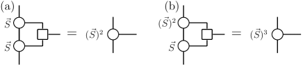
Figure S5: Demonstration on how to obtain $(\vec{S})^{2}$ and $(\vec{S})^{3}$ operators via the fusion process. The fusion matrix (3-leg square tensor) is the identity matrix of the fusion process $q_{i}\bigotimes q_{j}=\bigoplus q_{k}$.

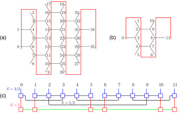
Figure S6: Path taken through a spin cluster in order to represent its ground state and excitations by MPSs; (a) the 36-site cluster on which our proof is based and (b) a smaller 12-site illustrative cluster. The MPS representing a 2D AKLT state on the path is made out of two layers of MPSs in (c); the top layer (blue) reproduces the 2D lattice connectivity, with the boxes correspond to the tensors $T$ [which incorporate $\mathrm{SU}(2)$ symmetry via the $B$ and $C$ tensors discussed in the text]. In the lower layer, red lines and boxes represent $S=1$ free boundary spins and the green lines show one of the non-repeating paths that fuse all $S=1$ into a total angular moment $J$.

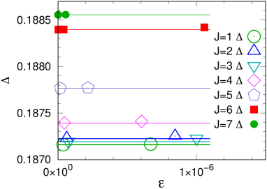
Figure S7: The smallest nonzero gaps in the sectors $1\leq J\leq L+1=7$ vs the discarded weight in DMRG calculations for the open-boundary 12-sites AKLT cluster in Fig. S6(b) with the bond weights in Eq. (5) taken to be $w_{e}=1.2$ on the central hexagon and $w_{e}=1$ on the edges connecting to the boundary dangling spins. The solid lines indicate the corresponding exact results from Lanczos diagonalization. The case $J=0$ is not shown here because that gap is much larger, but our method also reproduces it very well. The smallest gap is in the $J=1$ sector.

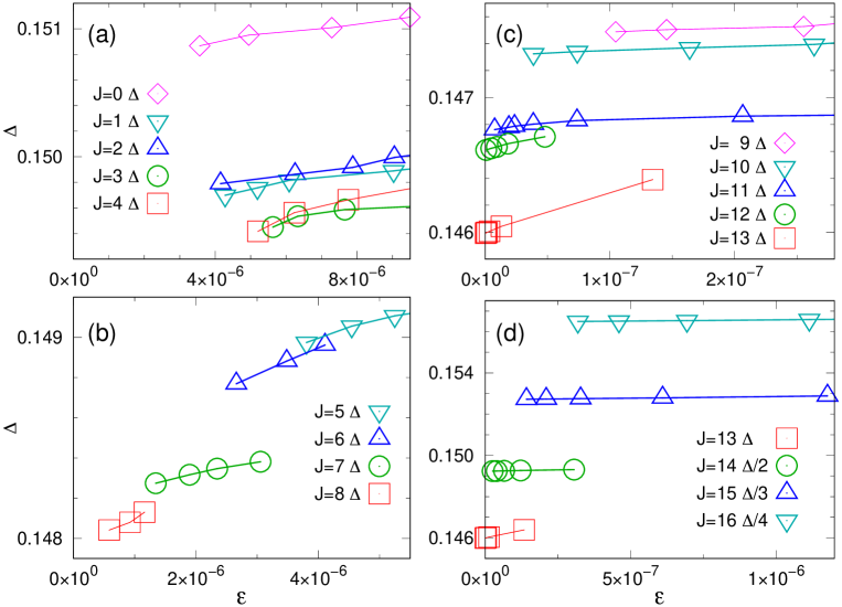
Figure S8: The smallest nonzero gaps in the sectors $0\leq J\leq L+4=16$ vs the discarded weight in DMRG calculations for the open-boundary 36-sites cluster depicted in Fig. 2 of the main paper. Here the value of the adjustable bulk coupling is $a=1.4$, which is the value for which we have proved the finite-size criterion. The solid lines drawn through the $J=13$ points in (b) and (d) are linear fits giving the extrapolated gap $\Delta(13)=0.14599$. The lines between points for other $J$ values are only guides to the eye. Note that, in (d) the gaps have been divided by $J-12$ in order to compress the horizontal scale (also demonstrating that the gaps for large $J$ scale roughly as $J+1-L$ in this case). The maximum bond dimension (corresponding to the smallest $\epsilon$ for each $J$) is $D=2000$ in panel (a), $D=2400$ for $5\leq J\leq 12$, and $D=1200$ for all other cases.

Given an operator $\hat{O}_{q_{i}}$ in its $\mathrm{SU}(2)$ invariant form, its basis transformation is guaranteed to preserve the same form, as demonstrated in Fig. S4. The spin operator

$$\left(-\frac{1}{\sqrt{2}}S^{+},S^{z},\frac{1}{\sqrt{2}}S^{-}\right)^{T}$$ (S20)

transforms like a wavefunction with angular moment 1. To realize the AKLT Hamiltonian Eq. (S13) written in terms of vector operators $(\vec{S})^{1}$, $(\vec{S})^{2}$, and $(\vec{S})^{3}$, requires implementing their $\mathrm{SU}(2)$ invarient representations. For example, $(\vec{S}^{2})$ is constructed simply by multiplying two $\vec{S}$ operators on the physical index and successively fusing two $q=1$ angular momenta on the virtual index into a total angular momentum $q=0,1,2$, following the fusion rule $1\otimes 1=0\oplus 1\oplus 2$, as shown in Fig. S5(a). Similarly, $(\vec{S})^{3}$ can be constructed by multiplying $(\vec{S})^{2}$ and $\vec{S}$ on the physical index and fusing the virtual index, as in Fig. S5(b).

With the above preparation in an $\mathrm{SU}(2)$ invariant basis, one can enumerate the complete ground state manifold and computate the lowest excitation in each total spin $J$ sectors, which we here do for the 36-site 2D AKLT cluster depicted in Fig. 2 in the main text. For illustration purposes we will here also consider a 12-site cluster, for which it is easier to draw pictures of the MPSs incorporating the edge spins; Fig. S6.

The degenerate ground states of the cluster with open boundaries are generated by first preparing them in their 2D tensor network representation, as with the black solid lines in Figs. S6(a) and (b). Then, as always in 2D DMRG calculations, a path is chosen to ’snake’ through the 2D network to compress the states into MPSs. The paths chosen here for the two clusters are indicated with red lines. This type of path represents the minimum number of cuts when partitioning the system into two arbitrary parts. Minimizing the number of cuts optimizes the ability of the MPS to build in bipartite entanglement.

The compression procedure and special treatment of the boundary spins works as follows, using the 12-site system for definiteness in the illustration in Fig. S6(c). First, the ’snake’ is stretched into a line as shown with the blue boxes, which represent the $\mathrm{SU}(2)$ $T$ tensors discussed above. The connectivity of the original 2D network is shown with the black lines. The remaining dangling $S=1$ degrees of freedom form a set of unitary orthogonal MPSs with different total angular momenta; this MPS representation is shown with the red boxes. The green lines can connect these boxes in any non-repeating order, and a given path corresponds to a set of fusion values that define the quantum numbers associated with the line segments. The final MPS representing the 2D AKLT ground state is formulated by combining the two layers of matrix product states as in Fig. S6(c); a blue layer of all physical spins and a red layer of the dangling boundary spins.

All the paths [green lines in Fig. S6(c)] connecting the tensors of the lower layer have to be considered to construct the full ground state manifold. Generating these unitary orthogonal MPSs of the free $S=1$ boundary degrees of freedom is a computer facilitated automatic process that requires a computational effort scaling with the Hilbert space sizes for all possible $J$—these sizes are listed for the 36-site cluster in the main paper. Once all the ground state in a given sector $J$ has been gathered, one can employ the DMRG algorithm for excited states, as described in Ref. prl121.107202 , to compute the first excited state above the ground state manifold. In the case considered here the procedure is simplified due to the fact that the ground states are known exactly and are written out straight forwardly without any energy minimization.

III. DMRG gap convergence

We have carried out various tests to confirm the correctness of the DMRG code, e.g., using the 1D AKLT chain and smaller 2D clusters for which the gaps can be verified using Lanczos exact diagonalization. Even with the $\mathrm{SU}(2)$ symmetry implemented and all the degenerate ground state projected out exactly, reliably computing the gaps for all $J$ values of interest for a cluster with $36$ spins is not an easy task. Convergence as a function of the bond dimension $D$ has to be carefully checked. Instead of monitoring the convergence directly versus $D$, it is better to consider the energy as a function of the discarded weight $\epsilon$ of the DMRG procedure obtained for each $D$ used.

For the 12-site cluster in Fig. S6 we can easily compute the ground state in each $J$ sector by Lanczos exact diagonalization. We can then unambiguously test our DMRG method with the MPS-expressed degenerate ground states projected out exactly. Fig. S7 shows the results for several $J$ values versus the discarded DMRG weight $\epsilon$. The solid lines are the exact Lanczos results, and they agree very well with the DMRG results for small $\epsilon$. For this cluster the lowest gap is in the $J=1$ sector and there is no particular systematic ordering of the levels.

In Fig. S8 we show our results for the 36-site cluster. As discussed in the main text, we expect the smallest gap should be for $J\in\{0,1,\ldots,13\}$, but we carried out calculations for all possible $J$-values and confirmed that the gaps increase rapidly upon increasing $J$ above $J=13$. Since the values of $\epsilon$ for which extrapolations can reliably be carried out span a wide range, rather systematically depending on $J$, in Fig. S8 we have divided up the results for the different $J$ values into four different panels with groups of similar $J$ values. The reason for the larger $\epsilon$ for smaller $J$ is primarily due to the size of the Hilbert space, which increases with decreasing $J$.

Based on these results there is no doubt that the smallest gap of this cluster is in the $J=13$ sector. The gaps increase rapidly with $J$. We mention that the gaps in sectors of very large $J$ can also be estimated analytically, e.g., by using the projection lemma from KKR . For smaller $J$ the gaps initially increase monotonically, but for the $J\leq 4$ non-monotonic behavior sets in. There the gaps are already much larger than $\Delta(13)$.

References

• (1) F.D.M. Haldane, Continuum dynamics of the 1 -d Heisenberg antiferromagnet: identification with the $O(3)$ nonlinear sigma model, Phys. Lett. 93 (1983), 464 – 468
• (2) F.D.M. Haldane, Nonlinear field theory of large-spin Heisenberg antiferromagnets: semiclassically quantized solutions of the one-dimensional easy-axis Neel state, Phys. Rev. Lett. 50 (1983), 1153–1156
• (3) I. Affleck, T. Kennedy, E.H. Lieb, and H. Tasaki, Rigorous results on valence-bond ground states in antiferromagnets, Phys. Rev. Lett. 59 (1987), 799
• (4) I. Affleck, T. Kennedy, E.H. Lieb, and H. Tasaki, Valence Bond Ground States in Isotropic Quantum Antiferromagnets, Comm. Math. Phys. 115 (1988), no. 3, 477 – 528
• (5) A. Cichocki, N. Lee, I. Oseledets, A.-H. Phan, Q. Zhao, and D.P. Mandic, Tensor networks for dimensionality reduction and large-scale optimization: Part 1 low-rank tensor decompositions, Found. Trends Mach. Learn., 9 (2016), 249–429
• (6) A. Cichocki, N. Lee, I. Oseledets, A.-H. Phan, Q. Zhao, and D.P. Mandic, Tensor networks for dimensionality reduction and large-scale optimization: Part 2 low-rank tensor decompositions, Found. Trends Mach. Learn., 9 (2017), 431–673
• (7) M. Fannes, B. Nachtergaele, R.F. Werner, Finitely Correlated States on Quantum Spin Chains, Commun. Math. Phys. 144 (1992), 443–490
• (8) R. Orus, A Practical Introduction to Tensor Networks: Matrix Product States and Projected Entangled Pair States, Ann. Phys. 349 (2014) 117–158
• (9) U. Schollwöck, The density-matrix renormalization group in the age of matrix product states, Ann. Phys. 326 (2011), 96–192
• (10) N. Schuch, M.M. Wolf, F. Verstraete, and J.I. Cirac, Computational Complexity of Projected Entangled Pair States, Phys. Rev. Lett. 98 (2007), 140506
• (11) N. Schuch, I. Cirac, D. Perez-Garcia, PEPS as ground states: degeneracy and topology, Ann. Phys. 325 (2010), 2153
• (12) T. Kennedy, and H. Tasaki, Hidden symmetry breaking and the Haldane phase in $S=1$ quantum spin chains , Comm. Math. Phys. 147 (1992), no. 3, 431–484
• (13) M. den Nijs and K. Rommelse, Preroughening transitions in crystal surfaces and valence-bond phases in quantum spin chains, Phys. Rev. B 40 (1989), 4709
• (14) F. Pollmann, A.M. Turner, E. Berg, and M. Oshikawa, Entanglement spectrum of a topological phase in one dimension, Phys. Rev. B 81 (2010), 064439
• (15) X. Chen, Z.-C. Gu, Z.-X. Liu, X.-G. Wen, Symmetry-Protected Topological Orders in Interacting Bosonic Systems Science 338 (2012), no. 6114, 1604–1606
• (16) L. Fidkowski, and A. Kitaev Topological phases of fermions in one dimension, Phys. Rev. B 83 (2011), 075103
• (17) T. Morimoto, H. Ueda, T. Momoi, and A. Furusaki, $\mathbb{Z}^{3}$ symmetry-protected topological phases in the $\mathrm{SU}(3)$ AKLT model, Phys. Rev. B 90 (2014), 235111
• (18) Z. Nussinov, and G. Ortiz, A symmetry principle for topological quantum order, Ann. Phys. 324 (2009), no. 5, 977–1057
• (19) F. Verstraete, J.I. Cirac, Valence Bond Solids for Quantum Computation, Phys. Rev. A 70 (2004), 060302(R)
• (20) A. Miyake, Quantum computational capability of a 2D valence bond solid phase, Ann.  Phys. 326 (2011), no. 7, 1656–1671
• (21) T-C. Wei, I. Affleck, and R. Raussendorf, Affleck-Kennedy-Lieb-Tasaki state on a honeycomb lattice is a universal quantum computational resource, Phys. Rev. Lett. 106 (2011), 070501.
• (22) T-C. Wei, P. Haghnegahdar, and R. Raussendorf, Hybrid valence-bond states for universal quantum computation, Phys. Rev. A 90 (2014), 042333
• (23) T. Kennedy, E.H. Lieb, and H. Tasaki, A two-dimensional isotropic quantum antiferromagnet with unique disordered ground state, J. Stat. Phys. 53 (1988), 383 – 415.
• (24) C. Fernandez-Gonzalez, N. Schuch, M.M. Wolf, J.I. Cirac, D. Perez-Garcia, Frustration Free Gapless Hamiltonians for Matrix Product States, Comm. Math. Phys. 333 (2015), 299–333
• (25) C. Fernandez-Gonzalez, N. Schuch, M.M. Wolf, J.I. Cirac, D. Perez-Garcia, Gapless Hamiltonians for the Toric Code Using the Projected Entangled Pair State Formalism, Phys. Rev. Lett. 109 (2012), 260401
• (26) M. Hastings, T. Koma, Spectral gap and exponential decay of correlations, Comm. Math. Phys. 265 (2006), no. 3, 781–804
• (27) B. Nachtergaele, The spectral gap for some spin chains with discrete symmetry breaking, Comm. Math. Phys. 175 (1996), no. 3, 565–606.
• (28) B. Nachtergaele, and R. Sims, Lieb-Robinson bounds and the exponential clustering theorem, Comm. Math. Phys. 265 (2006), no. 1, 119 – 130
• (29) H. Abdul-Rahman, M. Lemm, A. Lucia, B.  Nachtergaele, and A. Young, A class of two-dimensional AKLT models with a gap, Analytic trends in mathematical physics, Contemp. Math. 741, 1, Amer. Math. Soc., Providence, RI 2020
• (30) A.S. Darmawan and S.D. Bartlett, Spectral properties for a family of two-dimensional quantum antiferromagnets, Phys. Rev. B 93 (2016), 045129
• (31) A. Garcia-Saez, V. Murg, and T.-C. Wei, Spectral gaps of Affleck-Kennedy-Lieb-Tasaki Hamiltonians using tensor network methods, Phys. Rev. B 88 (2013), 245118
• (32) S. Knabe, Energy gaps and elementary excitations for certain VBS-quantum antiferromagnets, J. Stat. Phys. 52 (1988), no. 3-4, 627 – 638
• (33) M. Lemm, A. Sandvik, and S. Yang, The AKLT model on a hexagonal chain is gapped, J. Stat. Phys. 177 (2019), no. 6, 1077-1088
• (34) N. Pomata, T.-C. Wei, AKLT models on decorated square lattices are gapped, Phys. Rev. B 100 (2019), 094429
• (35) J.I. Cirac, J. Garre-Rubio, D. Perez-Garcia Mathematical open problems in projected entangled pair states, Rev. Mat. Complut. 32 (2019), 32, no. 3, 579–599
• (36) M. Lemm and B. Nachtergaele, Gapped PVBS models for all species numbers and dimensions, Rev. Math. Phys. 31 (2019), no. 9, 1950028
• (37) S. Bachmann, E. Hamza, B. Nachtergaele and A. Young, Product Vacua and Boundary State Models in $d$ Dimensions, J. Stat. Phys. 160 (2015), 636–658
• (38) M. Bishop, Spectral gaps for the Two-Species Product Vacua and Boundary States models on the $d$-dimensional lattice, J. Stat. Phys. 175 (2019), no. 2, 418–455
• (39) D. Gosset and E. Mozgunov, Local gap threshold for frustration-free spin systems, J. Math. Phys. 57 (2016), 091901
• (40) M. Lemm and E. Mozgunov, Spectral gaps of frustration-free spin systems with boundary, J. Math. Phys. 60 (2019) 051901
• (41) See Supplemental Material for details of the proof of the finite-size criterion, implementation of the $\mathrm{SU}(2)$ DMRG algorithm for the AKLT model, and convergence properties of the gaps.
• (42) A. Anshu, Improved local spectral gap thresholds for lattices of finite size, Phys. Rev. B 101 (2020), 165104
• (43) M. Lemm, Gaplessness is not generic for translation-invariant spin chains, Phys. Rev. B 100 (2019) 035113
• (44) M. Lemm, Finite-size criteria for spectral gaps in D-dimensional quantum spin systems, Contemp. Math. 741, 121, Amer. Math. Soc., Providence, RI 2020
• (45) L. Wang, and A. W. Sandvik, Critical Level Crossings and Gapless Spin Liquid in the Square-Lattice Spin-$1/2$ $J_{1}$-$J_{2}$ Heisenberg Antiferromagnet, Phys. Rev. Lett. 121 (2018), 107202
• (46) S. Bachmann, A. Bols, W. De Roeck, M. Fraas, Quantization of Conductance in Gapped Interacting Systems, Ann. Henri Poincaré 19, 695–708 (2018)
• (47) S. Bachmann, S. Michalakis, B. Nachtergaele, and R. Sims, Automorphic equivalence within gapped phases of quantum lattice systems, Comm. Math. Phys. 309 (2012), no. 3, 835 – 871
• (48) S. Bravyi, M. Hastings, S. Michalakis, Topological quantum order: stability under local perturbations, J. Math. Phys. 51 (2010), 093512
• (49) M.B. Hastings, Lieb-Schultz-Mattis in higher dimensions Phys. Rev. B 69 (2004),104431
• (50) M.B. Hastings and X.-G. Wen, Quasiadiabatic continuation of quantum states: The stability of topological ground-state degeneracy and emergent gauge invariance, Phys. Rev. B, 72, (2005), no. 4, 045141
• (51) S. Bachmann, W. De Roeck, and M. Fraas, Adiabatic Theorem for Quantum Spin Systems, Phys. Rev. Lett. 119 (2017), 060201
• (52) M.B. Hastings, The stability of free Fermi Hamiltonians J. Math. Phys. 60 (2019), no. 4, 042201
• (53) W. De Roeck, and M. Salmhofer, Persistence of exponential decay and spectral gaps for interacting fermions Comm. Math. Phys., 365, no. 2, 773–796
• (54) J. Fröhlich, and A. Pizzo, Lie–Schwinger block-diagonalization and gapped quantum chains to appear in Comm. Math. Phys., (2020)
• (55) S. Michalakis, and J. Zwolak, Stability of frustration-free Hamiltonians, Comm. Math. Phys. 322 (2013), no. 2, 277 – 302
• (56) D.P. Arovas, A. Auerbach, F.D.M. Haldane, Extended Heisenberg models of antiferromagnetism: Analogies to the fractional quantum Hall effect, Phys. Rev. Lett. 60 (1988), 531
• (57) M. Greiter, and S. Rachel., Valence bond solids for $\mathrm{SU}(N)$ spin chains: exact models, spinon confinement, and the Haldane gap, Phys. Rev.  B 75 (2007), 184441
• (58) K. Wan, P. Nataf, and F. Mila. Exact diagonalization of $\mathrm{SU}(N)$ Heisenberg and Affleck-Kennedy-Lieb-Tasaki chains using the full $\mathrm{SU}(N)$ symmetry, Phys. Rev.  B 96 (2017), 115159
• (59) O. Gauthé, D. Poilblanc, Entanglement properties of the two-dimensional $\mathrm{SU}(3)$ Affleck-Kennedy-Lieb-Tasaki state, Phys. Rev.  B 96 (2017), 121115.
• (60) S.A. Parameswaran, S.L. Sondhi, and D.P. Arovas, Order and disorder in AKLT antiferromagnets in three dimensions, Phys. Rev. B 79 (2009), 024408
• (61) N. Pomata, T.-C. Wei, Demonstrating the Affleck-Kennedy-Lieb-Tasaki Spectral Gap on 2D Degree-3 Lattices, Phys. Rev. Lett. 124 (2020), 177203
• (62) A. Weichselbaum, Non-abelian symmetries in tensor networks: a quantum symmetry space approach, Ann. Phys. 327, 2972 (2012)
• (63) J. Kempe, A. Kitaev, O. Regev, The Complexity of the Local Hamiltonian Problem, SIAM J. Comput., 35(5), 1070–1097