A damped forward–backward algorithm for stochastic generalized Nash equilibrium seeking

Abstract

We consider a stochastic generalized Nash equilibrium problem (GNEP) with expected–value cost functions. Inspired by Yi and Pavel (Automatica, 2019), we propose a distributed GNE seeking algorithm by exploiting the forward–backward operator splitting and a suitable preconditioning matrix. Specifically, we apply this method to the stochastic GNEP, where, at each iteration, the expected value of the pseudo–gradient is approximated via a number of random samples. Our main contribution is to show almost sure convergence of our proposed algorithm if the sample size grows large enough.

I Introduction

Generalized Nash equilibrium problems (GNEPs) have been widely studied in the literature. Many results are present concerning algorithms and methodologies to find an equilibrium [1, 2] (and the references therein). The reason for this interest is related with the potential applications ranging from economics to engineering via operation research [3, 4]. In a GNEP, each agent aims at minimizing his own cost function, under some feasibility constraints. The main feature is that both the cost function and the constraints depend on the stategy chosen by the other agents. Due to the presence of shared constraints, the search for a generalized Nash equilibrium is a challenging task in general.

In the deterministic case, several algorithms are available for finding a GNE, both distributed and semi-decentralized [1, 5, 6, 7]. Among the available methods for GNEP, an elegant approach is to recast the problem as a monotone inclusion through the use of interdependent Karush–Kuhn–Tucker (KKT) conditions. The resulting Lagrangian formulation allows one to seek equilibrium points as the solutions of an associated variational inequality (VI) that is usually more tractable and the literature is wider than the GNEPs literature [8, 2] (and reference therein). Equilibria obtained in this way are called variational equilibria.

Given a monotone inclusion problem, a powerful procedure is to use an operator splitting scheme to recast the problem as the search for the zeros of a sum of two monotone operators. One of the simplest schemes is the forward–backward (FB) operator splitting [8]. Convergence of such a scheme is guaranteed if the pseudo-gradient mapping of the game is strongly monotone. Since we study a game-theoretic problem, the algorithm should be distributed, in the sense that each agent should only know his local cost function and his local constraints. Unfortunately, the FB splitting does not lead to a distributed algorithm when applied to a GNEP. In the deterministic case, preconditioning has been proposed in [5, 6] to overcome this problem. To the best of our knowledge, the preconditioned FB operator splitting has not been exploited for stochastic GNEPs (SGNEPs) but it would be very relevant from an algorithmic perspective.

The literature on stochastic Nash equilibrium problems is less rich than its deterministic counterpart [9, 10, 11]. However, several problems of interest cannot be modelled without uncertainty. Among others, consider transportation systems, where one source of uncertainty is due to the drivers perception of travel time [12]; electricity markets where generators produce energy without knowing the actual demand [13]; or, more generally, problems that can be modelled as networked Cournot games with market capacity constraints where the demand is uncertain [14, 15]. Mathematically speaking, a SGNEP is a GNEP where the cost functions of the agents are expected–value functions and the distribution of the random variables is unknown. Existence (and uniqueness) of equilibria is studied in [10] but the study of convergent algorithms is not fully developed yet [11, 9].

One possible motivation for this lack of results is the presence of the expected–value cost functions. When the probability distribution of the random variable is known, the expected value formulation can be solved with a technique for deterministic VI. However, the pseudo gradient is usually not directly accessible, for instance due to the intractability of computing the expected value. For this reason, in many cases, the solution of a stochastic VI relies on samples of the random variable. There are, in fact, two main methodologies available: sample average approximation (SAA) and stochastic approximation (SA). The SAA approach replaces the expected value with the average over a huge number of samples of the random variable. This approach is practical in Monte Carlo Simulations or machine learning, when there is a huge number of data available [16, 17]. In the SA approach, the decision maker draws only one sample of the random variable. This approach is less computationally expensive and more appropriate in a decentralized framework but, in general, it requires stronger assumptions of the problem data [18, 19, 20].

In this paper, we formulate a distributed stochastic FB algorithm through preconditioning and prove its consequent convergence. The associated SVI is obtained in the same way as the deterministic case, i.e., via augmented KKT inclusions. Among the possible approaches for solving an SVI [18, 17, 19], we propose a damped forward–backward scheme [21] and prove convergence under proper assumptions, i.e., strong monotonicity of the pseudo gradient game mapping and measurability of the random variable.

Notation: We use Standing Assumptions to state technical conditions that implicitly hold throughout the paper while Assumptions are postulated only when explicitly used.

$\langle\cdot,\cdot\rangle:{\mathbb{R}}^{n}\times{\mathbb{R}}^{n}\to{\mathbb{R}}$ denotes the standard inner product and $\left\|\cdot\right\|$ is the associated euclidean norm. We indicate that a matrix $A$ is positive definite, i.e., $x^{\top}Ax>0$, with $A\succ 0$. $A\otimes B$ indicates the Kronecker product between matrices $A$ and $B$. Given a symmetric $\Phi\succ 0$, the $\Phi$-induced inner product is $\langle x,y\rangle_{\Phi}=\langle\Phi x,y\rangle$. The associated $\Phi$-induced norm is defined as $\left\|x\right\|_{\Phi}=\sqrt{\langle\Phi x,x\rangle}$. ${\bf{0}}_{m}$ indicates the vector with $m$ entries all equal to $0$. Given $x_{1},\ldots,x_{N}\in{\mathbb{R}}^{n},\bm{x}:=\operatorname{col}\left(x_{1},\dots,x_{N}\right)=\left[x_{1}^{\top},\dots,x_{N}^{\top}\right]^{\top}$. $\operatorname{J}_{F}=(\operatorname{Id}+F)^{-1}$ is the resolvent of the operator $F$ where $\operatorname{Id}$ is the identity operator. For a closed set $C\subseteq{\mathbb{R}}^{n},$ the mapping $\operatorname{proj}_{C}:{\mathbb{R}}^{n}\to C$ denotes the projection onto $C$, i.e., $\operatorname{proj}_{C}(x)=\operatorname{argmin}_{y\in C}\|y-x\|$. $\iota_{C}$ is the indicator function of the set C, that is, $\iota_{C}(x)=1$ if $x\in C$ and $\iota_{C}(x)=0$ otherwise. The set-valued mapping $\mathrm{N}_{C}:{\mathbb{R}}^{n}\to{\mathbb{R}}^{n}$ denotes the normal cone operator of the set $C$ , i.e., $\mathrm{N}_{C}(x)=\varnothing$ if $x\notin C,\left\{v\in{\mathbb{R}}^{n}|\sup_{z\in C}v^{\top}(z-x)\leq 0\right\}$ otherwise. Given $\psi:{\mathbb{R}}^{n}\to{\mathbb{R}}$, $\operatorname{dom}(\psi):=\{x\in{\mathbb{R}}^{n}|\psi(x)<\infty\}$ is the domain and the subdifferential is the set-valued mapping $\partial\psi(x):=\{v\in{\mathbb{R}}^{n}|\psi(z)\geq\psi(x)+v^{\top}(z-x)\forall z\in\operatorname{dom}(\psi)\}$.

II Generalized Nash equilibrium problem

II-A Equilibrium Problem setup

We consider a set $\mathcal{I}=\{1,\dots,N\}$ of agents, each of them deciding on its action variable $x_{i}\in{\mathbb{R}}^{n_{i}}$ from its local decision set $\Omega_{i}\in{\mathbb{R}}^{n_{i}}$ with the aim of minimizing its local cost function. Let $\bm{x}_{-i}=\operatorname{col}((x_{j})_{j\neq i})$ be the decisions of all the agents except for $i$ and define $n=\sum_{i=1}^{N}n_{i}$. We consider that there is some uncertainty in the cost function, expressed through the random variable $\xi:\Xi\to{\mathbb{R}}^{d}$, where $(\Xi,\mathcal{F},{\mathbb{P}})$ is the associated probability space. Then, for each agent $i\in\mathcal{I}$, we define the cost function ${\mathbb{J}}_{i}:{\mathbb{R}}^{n}\rightarrow{\mathbb{R}}$ as

$${\mathbb{J}}_{i}(x_{i},\bm{x}_{-i}):={\mathbb{E}}_{\xi}[J_{i}(x_{i},\bm{x}_{-i},\xi(\omega))]\vspace{-.15cm}$$ (1)

for some measurable function $J_{i}:\mathcal{{\mathbb{R}}}^{n}\times{\mathbb{R}}^{d}\to{\mathbb{R}}$. We note that the cost function depends on the local variable $x_{i}$, the collective decision of the other agents $\bm{x}_{-i}$ (or a subset) and the random variable $\xi(\omega)$. ${\mathbb{E}}_{\xi}$ represents the mathematical expectation with respect to the distribution of the random variable $\xi$. We assume that ${\mathbb{E}}[J_{i}(\bm{x},\xi)]$ is well defined for all the feasible $\bm{x}=\operatorname{col}(x_{1},\dots,x_{N})$. Furthermore, we consider a game with affine shared constraints, $A\bm{x}\leq b$. Thus we denote the feasible decision set of each agent $i\in\mathcal{I}$ by the set-valued mapping

$$\mathcal{X}_{i}(\bm{x}_{-i}):=\left\{y_{i}\in\Omega_{i}\;|\;\textstyle{A_{i}y_{i}\leq b-\sum_{j\neq i}^{N}A_{j}x_{j}}\right\},\vspace{-.15cm}$$ (2)

where $A_{i}\in{\mathbb{R}}^{m\times n_{i}}$ and $b\in{\mathbb{R}}^{m}$. The matrix $A_{i}$ defines how agent $i$ is involved in the coupling constraints. The collective feasible set can be then written as

$$\bm{\mathcal{X}}=\bm{\Omega}\cap\left\{\bm{y}\in{\mathbb{R}}^{n}|A\bm{y}-b\leq{\bf{0}}_{m}\right\}\vspace{-.15cm}$$ (3)

where $\bm{\Omega}=\prod_{i=1}^{N}\Omega_{i}$ and $A=\left[A_{1},\ldots,A_{N}\right]\in{\mathbb{R}}^{m\times n}$. Note that there is no uncertainty in the constraints.

Next, we postulate standard assumptions for the cost functions and the constraints set.

Standing Assumption 1

For each $i\in\mathcal{I}$ and $\bm{x}_{-i}\in\mathcal{X}_{-i}$ the function ${\mathbb{J}}_{i}(\cdot,\bm{x}_{-i})$ is convex and continuously differentiable. $\blacksquare$

Standing Assumption 2

For each $i\in\mathcal{I},$ the set $\Omega_{i}$ is nonempty, compact and convex. The set $\mathcal{X}$ satisfies Slater’s constraint qualification. $\blacksquare$

Formally, the aim of each agent $i$, given the decision variables of the other agents $\bm{x}_{-i}$, is to choose a action variable $x_{i}$, that solves its local optimization problem, i.e.,

$$\forall i\in\mathcal{I}:\quad\left\{\begin{array}[]{cl}\min_{x_{i}\in\Omega_{i}}&{\mathbb{J}}_{i}(x_{i},\bm{x}_{-i})\\ \text{ s.t. }&A_{i}x_{i}\leq b-\sum_{j\neq i}^{N}A_{j}x_{j}.\end{array}\right.\vspace{-.15cm}$$ (4)

From a game-theoretic perspective, we aim at computing a stochastic generalized Nash equilibrium (SGNE) [10], i.e., a collective variable $\bm{x}^{*}\in\mathcal{X}$ such that, for all $i\in\mathcal{I}$:

$${\mathbb{J}}_{i}(x_{i}^{*},\bm{x}_{-i}^{*})\leq\inf\{{\mathbb{J}}_{i}(y,\bm{x}_{-i}^{*})\;|\;y\in\mathcal{X}_{i}(\bm{x}_{-i}^{*})\}.\vspace{-.2cm}$$

In other words, a SGNE is a set of strategies where no agent can decrease its objective function by unilaterally changing its decision variable. To guarantee existence of a stochastic equilibrium, let us introduce further assumptions on the local cost functions $J_{i}$.

Standing Assumption 3

For each $i\in\mathcal{I}$ and $\xi\in\Xi$, the function $J_{i}(\cdot,\bm{x}_{-i},\xi)$ is convex, Lipschitz continuous, and continuously differentiable. The function $J_{i}(x_{i},\bm{x}_{-i},\cdot)$ is measurable and for each $\bm{x}_{-i}$, the Lipschitz constant $\ell_{i}(\bm{x}_{-i},\xi)$ is integrable in $\xi.$ $\blacksquare$

While, under Standing Assumptions 1, 2 and 3, existence of a GNE of the game is guaranteed by [10, §3.1], uniqueness does not hold in general [10, §3.2].

Within all possible Nash equilibria, we focus on those that corresponds to the solutions of an appropriate (stochastic) variational inequality. Let

$${\mathbb{F}}(\bm{x})=\operatorname{col}\left({\mathbb{E}}[\nabla_{x_{i}}J_{i}(x_{i},\bm{x}_{-i})]_{i\in\mathcal{I}}\right).\vspace{-.15cm}$$ (5)

Formally, the stochastic variational inequality problem $\operatorname{SVI}(\bm{\mathcal{X}},{\mathbb{F}})$ is the problem of finding $\bm{x}^{*}\in\bm{\mathcal{X}}$ such that

$$\langle{\mathbb{F}}(\bm{x}^{*}),\bm{x}-\bm{x}^{*}\rangle\geq 0,\;\text{ for all }\bm{x}\in\bm{\mathcal{X}}.\vspace{-.15cm}$$ (6)

with ${\mathbb{F}}(\bm{x})$ as in (5). We note that we can exchange the expected value and the gradient in (5) thanks to Standing Assumption 3 [10, Lem. 3.4]. We also note that any solution of $\operatorname{SVI}(\mathcal{X},{\mathbb{F}})$ is a generalized Nash equilibrium of the game in (4) while the opposite does not hold in general. In fact, a game may have a Nash equilibrium while the corresponding VI may have no solution [22, Prop. 12.7].

A sufficient condition for the variational problem in (6) to have a solution is that ${\mathbb{F}}$ is strongly monotone [2, Th. 2.3.3], [10, Lemma 3.3], as we postulate next.

Standing Assumption 4

${\mathbb{F}}$ is $\eta$-strongly monotone, i.e., for $\eta>0$, $\langle{\mathbb{F}}(x)-{\mathbb{F}}(y),x-y\rangle\geq\eta\left\|x-y\right\|^{2}$ for all $x,y\in{\mathbb{R}}^{n}$ and $\ell$-Lipschitz continuous, i.e., for $\ell>0$, $\left\|{\mathbb{F}}(x)-{\mathbb{F}}(y)\right\|\leq\ell\left\|x-y\right\|$ for all $x,y\in{\mathbb{R}}^{n}$. $\blacksquare$

II-B Operator-theoretic characterization

In this subsection, we recast the GNEP into a monotone inclusion, namely, the problem of finding a zero of a set-valued monotone operator.

First, we characterize the SGNE of the game in terms of the Karush–Kuhn–Tucker (KKT) conditions for the coupled optimization problems in (4). For each agent $i\in\mathcal{I}$, let us introduce the Lagrangian function $\mathcal{L}_{i}\left(\bm{x},\lambda_{i}\right):={\mathbb{J}}_{i}(x_{i},\bm{x}_{-i})+\iota_{\Omega_{i}}\left(x_{i}\right)+\lambda_{i}^{\top}(A\bm{x}-b)$, where $\lambda_{i}\in{\mathbb{R}}_{\geq 0}^{m}$ is the dual variable associated with the coupling constraints. We recall that the set of strategies $\bm{x}^{*}$ is a SGNE if and only if the following KKT conditions are satisfied [1, Th. 4.6]: for all $i\in\mathcal{I}$

$$\left\{\begin{array}[]{l}0\in{\mathbb{E}}[\nabla_{x_{i}}J_{i}(x_{i}^{*},\bm{x}_{-i}^{*},\xi)]+\mathrm{N}_{\Omega_{i}}\left(x_{i}^{*}\right)+A_{i}^{\top}\lambda_{i}\\ 0\in-(A\bm{x}^{*}-b)+\mathrm{N}_{{\mathbb{R}}^{m}_{\geq 0}}(\lambda^{*}).\end{array}\right.\vspace{-.15cm}$$ (7)

Similarly, we can use the KKT conditions to characterize a variational GNEP (v-GNEP), studying the Lagrangian function associated to the SVI. Since $\bm{x}^{*}$ is a solution of $\operatorname{SVI}(\bm{\mathcal{X}},{\mathbb{F}})$ if and only if $\bm{x}^{*}\in\operatorname{argmin}\limits_{\bm{y}\in\mathcal{X}}\left(\bm{y}-\bm{x}^{*}\right)^{\top}{\mathbb{F}}\left(\bm{x}^{*}\right),$ the associated KKT optimality conditions are, for all $i\in\mathcal{I}$

$$\left\{\begin{array}[]{l}0\in{\mathbb{E}}[\nabla_{x_{i}}J_{i}(x_{i}^{*},\bm{x}_{-i}^{*},\xi)]+\mathrm{N}_{\Omega_{i}}\left(x_{i}^{*}\right)+A_{i}^{\top}\lambda,\\ 0\in-(A\bm{x}^{*}-b)+\mathrm{N}_{{\mathbb{R}}^{m}_{\geq 0}}(\lambda^{*}).\end{array}\right.\vspace{-.15cm}$$ (8)

We note that (8) can be written in compact form as

$$0\in\mathcal{T}(\bm{x},\bm{\lambda}):=\left[\begin{array}[]{c}\mathrm{N}_{\Omega}(\bm{x})+{\mathbb{F}}(\bm{x})+A^{\top}\lambda\\ \mathrm{N}_{{\mathbb{R}}_{\geq 0}^{m}}(\lambda)-(A\bm{x}-b)\end{array}\right],\vspace{-.15cm}$$

where $\mathcal{T}:\bm{\mathcal{X}}\times{\mathbb{R}}^{m}_{\geq 0}\rightrightarrows{\mathbb{R}}^{n}\times{\mathbb{R}}^{m}$ is a set-valued mapping. It follows that the v-GNE correspond to the zeros of the mapping $\mathcal{T}$. The next proposition shows the relation between SGNE and variational equilibria.

Lemma 1

[23, Th. 3.1] The following statements hold:

1. Let $\bm{x}^{*}$ be a solution of ${\mathrm{SVI}}(\mathcal{X},{\mathbb{F}})$ at which the KKT conditions (8) hold. Then $\bm{x}^{*}$ is a solution of the SGNEP at which the KKT conditions (7) hold with $\lambda_{1}=\lambda_{2}=\dots=\lambda_{N}=\lambda^{*}$

2. Viceversa, let $\bm{x}^{*}$ be a solution of the SGNEP at which KKT conditions (7) hold with $\lambda_{1}=\lambda_{2}=\dots=\lambda_{N}=\lambda^{*}$. Then, $\bm{x}^{*}$ is a solution of $\operatorname{SVI}(\mathcal{X},{\mathbb{F}})$. $\blacksquare$

Essentially, Lemma 1 says that variational equilibria are those such that the shared constraints have the same dual variable for all the agents.

III Preconditioned forward–backward generalized Nash equilibrium seeking

In this section, we propose a distributed forward–backward algorithm for finding variational equilibria of the game in (4).

We suppose that each agent $i$ only knows its local data, i.e., $\Omega_{i}$, $A_{i}$ and $b_{i}$. Moreover, each player is able to compute, given $\operatorname{col}(x_{i},\bm{x}_{-i})$, ${\mathbb{E}}[\nabla_{x_{i}}J_{i}(x_{i},\bm{x}_{-i},\xi)]$ (or an approximation, as exploited later in the section). We assume therefore that each agent has access to the action variables that affect its local gradient (full information setup). These information can be retrieved, for each agent $i$, from the set $\mathcal{N}_{i}^{J}$, that is, the set of agents $j$ whose action $x_{j}$ explicitly influences ${\mathbb{J}}_{i}$.

Since, by Lemma 1, the configuration of the v-GNE requires consensus of the dual variables, we introduce an auxiliary variable $z_{i}\in{\mathbb{R}}^{m}$ for all $i\in\mathcal{I}$. The role of $\bm{z}=\operatorname{col}(z_{1},\dots,z_{N})$ is to enforce consensus but it does not affect the property of the operators and of the algorithm. More details on this variable are given in Section IV-A. The auxiliary variable and a local copy of the dual variable $\lambda_{i}$ are shared through the dual variables graph, $\mathcal{G}_{\lambda}=(\mathcal{I},\mathcal{E}_{\lambda})$. The set of edges $\mathcal{E}_{\lambda}$ represents the exchange of the private information on the dual variables: $(i,j)\in\mathcal{E}_{\lambda}$ if player $i$ can receive $\{\lambda_{j},z_{j}\}$ from player $j$. The set of neighbours of $i$ in $\mathcal{G}_{\lambda}$ is given by $\mathcal{N}_{i}^{\lambda}=\left\{j|(j,i)\in\mathcal{E}_{\lambda}\right\}$ [6, 9].

Standing Assumption 5

The dual variable graph is undirected and connected. $\blacksquare$

Each agent feasible set implicitly depends on all the other agents variables through the shared constraints. Thus, to reach consensus of the multipliers, all agents must coordinate and therefore, $\mathcal{G}_{\lambda}$ must be connected.

The weighted adjacency matrix of the dual variables graph is indicated with $W\in{\mathbb{R}}^{N\times N}$. Let $L=D-W\in{\mathbb{R}}^{N\times N}$ be the Laplacian matrix associated to the adjacency matrix $W$, where $D=\operatorname{diag}(d_{1},\dots,d_{N})$ is the diagonal matrix of the degrees and $d_{i}=\sum_{j=1}^{N}w_{i,j}$. It follows from Standing Assumption 5 that $W$ and the associated Laplacian $L$ are both symmetric, i.e., $W=W^{\top}$ and $L=L^{\top}$. Moreover, Standing Assumption 5 is fundamental to guarantee that the coupling constraints are satisfied since agents have to reach consensus of the dual variables.

Next we present a distributed forward–backward algorithm with damping for solving the SGNEP in (4) (Algorithm 1). For each agent $i$, the variables $x_{i}^{k}$, $z_{i}^{k}$ and $\lambda_{i}^{k}$ denote the local variables $x_{i}$, $z_{i}$ and $\lambda_{i}$ at the iteration time $k$ while $\alpha_{i}$, $\nu_{i}$ and $\sigma_{i}$ are the step sizes.

Algorithm 1 Distributed Stochastic Forward–Backward

Initialization: $x_{i}^{0}\in\Omega_{i},\lambda_{i}^{0}\in{\mathbb{R}}_{\geq 0}^{m},$ and $z_{i}^{0}\in{\mathbb{R}}^{m}.$
Iteration $k$: Agent $i$
(1): Receives $x_{j,k}$ for $j\in\mathcal{N}_{i}^{h},\lambda_{j}^{k}$ for $j\in\mathcal{N}_{i}^{\lambda}$ then updates:

$$\tilde{x}_{i}^{k}=\operatorname{proj}_{\Omega_{i}}[x_{i}^{k}-\alpha_{i}(\hat{F}_{i}(x_{i}^{k},\bm{x}_{-i}^{k},\xi_{i}^{k})-A_{i}^{\top}\lambda_{i}^{k})]$$

$$\tilde{z}_{i}^{k}=z_{i}^{k}+v_{i}\sum\nolimits_{j\in\mathcal{N}_{i}^{\lambda}}w_{i,j}(\lambda_{i}^{k}-\lambda_{j}^{k})$$

(2): Receives $z_{j,k+1}$ for all $j\in\mathcal{N}_{i}^{\lambda}$ then updates:

$$\tilde{\lambda}_{i}^{k}=\operatorname{proj}_{{\mathbb{R}}_{+}^{m}}\left[\lambda_{i}^{k}+\sigma_{i}\left(A_{i}(2\tilde{x}_{i}^{k}-x_{i}^{k})-b_{i}\right)\right.$$

$$\qquad+\sigma_{i}\sum\nolimits_{j\in\mathcal{N}_{i}^{\lambda}}w_{i,j}\left(2(\tilde{z}_{i}^{k}-\tilde{z}_{j}^{k})-(z_{i}^{k}-z_{j}^{k})\right)$$

$$\qquad-\sigma_{i}\sum\nolimits_{j\in\mathcal{N}_{i}^{\lambda}}\left.w_{i,j}(\lambda_{i}^{k}-\lambda_{j}^{k})\right]$$

$$x_{i}^{k+1}=(1-\delta)x_{i}^{k}+\delta\tilde{x}_{i}^{k}$$

$$z_{i}^{k+1}=(1-\delta)z_{i}^{k}+\delta\tilde{z}_{i}^{k}$$

$$\lambda_{i}^{k+1}=(1-\delta)\lambda_{i}^{k}+\delta\tilde{\lambda}_{i}^{k}$$

Since the distribution of the random variable is unknown, in the algorithm we have replaced the expected value with a sample average approximation (SAA). We assume to have access to a pool of i.i.d. sample realizations of the random variable collected, for all $k\in{\mathbb{N}}$ and for each agent $i\in\mathcal{I}$, in the vectors $\xi_{i}^{k}$. At each time $k$, we have

$$\hat{F}_{i}(x_{i}^{k},\bm{x}_{-i}^{k},\xi_{i}^{k}):=\frac{1}{N_{k}}\sum_{s=1}^{N_{k}}\nabla_{x_{i}}J_{i}(x_{i}^{k},\bm{x}_{-i}^{k},\xi_{i}^{(s)})\vspace{-.15cm}$$ (9)

where $N_{k}$ is the batch size. As usual in SAA, we assume that the batch size increases over time according to the following lower bound.

Assumption 1

There exist $c,k_{0},a>0$ such that, for all $k\in{\mathbb{N}}$, $N_{k}\geq c(k+k_{0})^{a+1}$. $\blacksquare$

We define the distance of the expected value and its approximation as $\epsilon^{k}=\hat{F}(\bm{x}^{k},\xi^{k})-{\mathbb{F}}(\bm{x}^{k})$.
Let us define the filtration $\mathcal{F}=\{\mathcal{F}_{k}\}$, that is, a family of $\sigma$-algebras such that $\mathcal{F}_{0}=\sigma\left(X_{0}\right)$, for all $k\geq 1$, $\mathcal{F}_{k}=\sigma\left(X_{0},\xi_{1},\xi_{2},\ldots,\xi_{k}\right)$ and $\mathcal{F}_{k}\subseteq\mathcal{F}_{k+1}$ for all $k\geq 0$. $\mathcal{F}$ collects the informations that each agent has at the beginning of iteration $k$. We note that the process $\epsilon_{k}$ is adapted to $\mathcal{F}$ and, therefore, satisfies the following assumption.

Assumption 2

For al $k\geq 0$, ${\mathbb{E}}\left[\epsilon_{k}|\mathcal{F}_{k}\right]=0$ a.s. $\blacksquare$

The stochastic error has a vanishing second moment.

Assumption 3

For all $k$ and $C>0$, the stochastic error is such that ${\mathbb{E}}[\|\epsilon^{k}\||\mathcal{F}_{k}]\leq C\sigma^{2}/N_{k}$. $\blacksquare$

Such a bound for the stochastic error can be obtained as a consequence of some milder assumptions that lay outside the scope of this work. We refer to [16, Lem. 4.2], [17, Lem. 3.12] for more details.

Furthermore, we assume that the step sizes are small enough as formalized next.

Standing Assumption 6

Let $\delta\in(0,1]$. Let $d_{i}=\sum_{j=1}^{N}w_{i,j}$ and define $d^{*}=\max_{i\in\mathcal{N}}\{d_{i}\}$. Let $0<\beta\leq\min\left\{\frac{1}{2d^{*}},\frac{\eta}{\ell^{2}}\right\},$ where $\eta$ and $\ell$ are respectively the strongly monotone and the Lipschitz constants as in Standing Assumption 4. The parameter $\tau$ is positive and $\tau<\frac{1}{2\beta}$. The step sizes $\alpha$, $\nu$ and $\sigma$ satisfy, for any agent $i$

$$0 <\alpha_{i}\leq\left(\max_{j=1,\ldots,n_{i}}\{\sum\nolimits_{k=1}^{m}|[A_{i}^{T}]_{jk}|\}+\tau\right)^{-1}$$ (10)

$$0 <\nu_{i}\leq\left(2d_{i}+\tau\right)^{-1}$$

$$0 <\sigma_{i}\leq\left(\max_{j=1,\ldots,m}\{\sum\nolimits_{k=1}^{k_{i}}|[A_{i}]_{jk}|\}+2d_{i}+\tau\right)^{-1}$$

where $[A_{i}^{\top}]_{jk}$ indicates the entry $(j,k)$ of the matrix $A_{i}^{\top}$. $\blacksquare$

Specifically, the choice of $\beta$ will be clear after Lemma 2. Besides the fact that the constant $\beta$ can be hard to compute, we note that the step sizes can be taken constant and each agent can independently choose its own.

We are now ready to state our convergence result.

Theorem 1

Let Assumptions 1 and 3 hold. Then, the sequence generated by Algorithm 1 with $\hat{F}_{i}$ as in (9) for all $i\in\mathcal{N}$ converges a.s. to a v-GNE of the game in (4).

Proof:

See Section IV. ∎

IV Convergence analysis

IV-A Preconditioned forward backward operator splitting

In this section, we prove convergence of Algorithm 1.

We first note that the mapping $\mathcal{T}$ can be written as the sum of two operators. Specifically, $\mathcal{T}=\mathcal{A}+\mathcal{B}$ where

$$\mathcal{A} :\left[\begin{array}[]{l}\bm{x}\\ \bm{\lambda}\end{array}\right]\mapsto\left[\begin{array}[]{c}{\mathbb{F}}(\bm{x})\\ b\end{array}\right]$$ (11)

$$\mathcal{B} :\left[\begin{array}[]{l}\bm{x}\\ \bm{\lambda}\end{array}\right]\mapsto\left[\begin{array}[]{c}\operatorname{N}_{\Omega}(\bm{x})\\ \operatorname{N}_{{\mathbb{R}}_{\geq 0}^{m}}(\lambda)\end{array}\right]+\left[\begin{array}[]{cc}0&A^{\top}\\ -A&0\end{array}\right]\left[\begin{array}[]{l}\bm{x}\\ \bm{\lambda}\end{array}\right].$$

We note that finding a solution of the variational SGNEP translates in finding $x^{*}\in\operatorname{zer}(\mathcal{A}+\mathcal{B})$.

Let $L$ be the Laplacian matrix of $\mathcal{G}_{\lambda}$ and set ${\bf{L}}=L\otimes\operatorname{I}_{m}\in{\mathbb{R}}^{Nm\times Nm}$. To impose consensus on the dual variables, the authors in [6] proposed the Laplacian constraint ${\bf{L}}\bm{\lambda}=0$. Then, to preserve monotonicity one can augment the two operators $\mathcal{A}$ and $\mathcal{B}$ introducing the auxiliary variable $\bm{z}$. Define ${\bf{A}}=\operatorname{diag}\{A_{1},\dots,A_{N}\}\in{\mathbb{R}}^{Nm\times n}$ and $\bm{\lambda}=\operatorname{col}(\lambda_{1},\dots,\lambda_{N})\in{\mathbb{R}}^{Nm}$ and similarly let us define $\bar{b}$ of suitable dimensions. Then, we introduce

$$\bar{\mathcal{A}} :\left[\begin{array}[]{l}\bm{x}\\ \bm{z}\\ \bm{\lambda}\end{array}\right]\mapsto\left[\begin{array}[]{c}{\mathbb{F}}(\bm{x})\\ 0\\ \bar{b}\end{array}\right]+\left[\begin{array}[]{c}0\\ 0\\ {\bf{L}}\bm{\lambda}\end{array}\right]$$ (12)

$$\bar{\mathcal{B}} :\left[\begin{array}[]{l}\bm{x}\\ \bm{z}\\ \bm{\lambda}\end{array}\right]\mapsto\left[\begin{array}[]{c}\operatorname{N}_{\Omega}(\bm{x})\\ {\bf{0}}_{mN}\\ \operatorname{N}_{{\mathbb{R}}_{\geq 0}^{m}}(\bm{\lambda})\end{array}\right]+\left[\begin{array}[]{ccc}0&0&{\bf{A}}^{\top}\\ 0&0&{\bf{L}}\\ -{\bf{A}}&-{\bf{L}}&0\end{array}\right]\left[\begin{array}[]{l}\bm{x}\\ \bm{z}\\ \bm{\lambda}\end{array}\right].$$

From now on, let us indicate $\bm{\omega}=\operatorname{col}(\bm{x},\bm{z},\bm{\lambda})$. The operators $\bar{\mathcal{A}}$ and $\bar{\mathcal{B}}$ in (12) have the following properties.

Lemma 2

The operator $\bar{\mathcal{B}}$ is maximally monotone and $\bar{\mathcal{A}}$ is $\beta$-cocoercive with $\beta$ as in Standing Assumption 6, i.e., $\langle\bar{\mathcal{A}}(x)-\bar{\mathcal{A}}(y),x-y\rangle\geq\beta\|\bar{\mathcal{A}}(x)-\bar{\mathcal{A}}(y)\|^{2}.$

Proof:

It follows from [6, Lem. 5]. ∎

Notice that this result explains the choice of the parameter $\beta$ in Assumption 6. The following lemma shows that the points $\bm{\omega}\in\operatorname{zer}(\bar{\mathcal{A}}+\bar{\mathcal{B}})$ provide a v-SGNE.

Lemma 3

Consider the operators $\bar{\mathcal{A}}$ and $\bar{\mathcal{B}}$ in (12), and the operators $\mathcal{A}$ and $\mathcal{B}$ in (11). Then the following hold.

• Given any $\bm{\omega}^{*}\in\operatorname{zer}(\bar{\mathcal{A}}+\bar{\mathcal{B}})$, $\bm{x}^{*}$ is a v-GNE of game in (4), i.e., $\bm{x}^{*}$ solves the ${\mathrm{SVI}}(\mathcal{X},{\mathbb{F}})$ in (6). Moreover $\bm{\lambda}^{*}=\mathbf{1}_{N}\otimes\lambda^{*},$ and $(\bm{x}^{*},\lambda^{*})$ satisfy the KKT condition in (8) i.e., $\operatorname{col}(\bm{x}^{*},\lambda^{*})\in\operatorname{zer}(\mathcal{A}+\mathcal{B})$

• $\operatorname{zer}(\mathcal{A}+\mathcal{B})\neq\emptyset$ and $\operatorname{zer}(\bar{\mathcal{A}}+\bar{\mathcal{B}})\neq\emptyset$

Proof:

It follows from [6, Th. 2]. ∎

Unfortunately, the operator $\bar{\mathcal{B}}$ is monotone but not cocoercive, due to the skew symmetric matrix, hence, we cannot directly apply the FB operator splitting [8, §26.5]. To overcome this issue, the authors in [6] introduced a preconditioning matrix $\Phi$. Thanks to $\Phi$, the zeros of the mapping $\mathcal{T}$ correspond to the fixed point of a specific operator that depends on the operators $\bar{\mathcal{A}}$ and $\bar{\mathcal{B}}$ as exploited in [5, 6]. Indeed, it holds that, for any matrix $\Phi\succ 0$, $\bm{\omega}\in\operatorname{zer}(\bar{\mathcal{A}}+\bar{\mathcal{B}})$ if and only if,

$$\bm{\omega}=\operatorname{J}_{\Phi^{-1}\bar{\mathcal{B}}}(\operatorname{Id}-\Phi^{-1}\bar{\mathcal{A}})(\bm{\omega})\vspace{-.15cm}$$ (13)

where $\operatorname{J}_{\Phi^{-1}\bar{\mathcal{B}}}=(\mathrm{Id}+\Phi^{-1}\bar{\mathcal{B}})^{-1}$ is the resolvent of $\bar{\mathcal{B}}$ and represent the backward step and $(\mathrm{Id}-\Phi^{-1}\bar{\mathcal{A}})$ is the (stochastic) forward step. In the deterministic case, convergence of the FB splitting is guaranteed by [8, Section 26.5]. In the stochastic case, the FB algorithm, as it is in (13), is known to converge for strongly monotone mappings [11]. For this reason, we focus on the following damped FB algorithm

$$\begin{cases}\tilde{\bm{\omega}}_{k}=\operatorname{J}_{\Phi^{-1}\bar{\mathcal{B}}}(\mathrm{Id}-\Phi^{-1}\bar{\mathcal{A}})(\bm{\omega}_{k})\\ \bm{\omega}_{k+1}=(1-\delta_{k})\bm{\omega}_{k}+\delta_{k}\tilde{\bm{\omega}}_{k}\end{cases}\vspace{-.15cm}$$ (14)

that converges with cocoercivity of $\Phi^{-1}\bar{\mathcal{A}}$ [21]. We show that this is true in Lemma 4.

First, we show that (14) is equivalent to Algorithm 1. Note that, if we write the resolvent explicitly, the first step of Equation (14) can be rewritten as

$$-\mathcal{\bar{A}}(\bm{\omega}^{k})\in\bar{\mathcal{B}}(\tilde{\bm{\omega}}^{k})+\Phi(\tilde{\bm{\omega}}^{k}-\bm{\omega}^{k}).\vspace{-.15cm}$$ (15)

The matrix $\Phi$ should be symmetric, positive definite and such that $\bm{\omega}_{k}$ is easy to be computed [5].

We define $\alpha^{-1}=\operatorname{diag}\{\alpha_{1}^{-1}\operatorname{I}_{n_{1}},\dots,\alpha_{N}^{-1}\operatorname{I}_{n_{N}}\}\in{\mathbb{R}}^{n\times n}$ and similarly $\sigma^{-1}$ and $\nu^{-1}$ of suitable dimensions. Let

$$\Phi=\left[\begin{array}[]{ccc}\alpha^{-1}&0&-{\bf{A}}^{\top}\\ 0&\nu^{-1}&-{\bf{L}}\\ -{\bf{A}}&-{\bf{L}}&\sigma^{-1}\end{array}\right]\vspace{-.15cm}$$ (16)

and suppose that the parameters $\alpha_{i}$, $\nu_{i}$ and $\sigma_{i}$ satisfy (10) in Standing Assumption 6.

We can obtain conditions (10) imposing $\Phi$ to be diagonally dominant. This, in combination with the fact that it is symmetric, implies that $\Phi$ is also positive definite. Then, the operators $\Phi^{-1}\bar{\mathcal{A}}$ and $\Phi^{-1}\bar{\mathcal{B}}$ satisfy the following properties under the $\Phi$-induced norm $\left\|\cdot\right\|_{\Phi}$.

Lemma 4

Given $\bar{\mathcal{A}}$ and $\bar{\mathcal{B}}$ in (12) and $\beta$ and $\tau$ as in Standing Assumption 6, the following statements hold:

• $\Phi^{-1}\bar{\mathcal{A}}$ is $\beta\tau$-cocoercive;

• $\Phi^{-1}\bar{\mathcal{B}}$ is maximally monotone.

Proof:

It follows from [6, Lem. 7]. ∎

IV-B Stochastic sample average approximation

Since the expected value can be hard to compute, we need to take an approximation. At this stage, it is not important if we use sample average or stochastic approximation, therefore, in what follows, we replace $\bar{\mathcal{A}}$ with

$$\hat{\mathcal{A}}:\left[\begin{array}[]{c}\bm{x}\\ \bm{z}\\ \bm{\lambda}\end{array}\right]\mapsto\left[\begin{array}[]{c}\hat{F}(\bm{x},\xi)\\ 0\\ \bar{b}\end{array}\right]+\left[\begin{array}[]{c}0\\ 0\\ {\bf{L}}\bm{\lambda}\end{array}\right]\vspace{-.15cm}$$

where $\hat{F}$ is an approximation of the expected value mapping ${\mathbb{F}}$ in (5) given a vector sample of the random variable $\xi$. Then, (15) can be rewritten as

$$-\left[\begin{array}[]{c}\hat{F}(\bm{x},\xi)\\ 0\\ {\bf{L}}\bm{\lambda}+\bar{b}\end{array}\right]\in \left[\begin{array}[]{ccc}0&0&{\bf{A}}^{\top}\\ 0&0&{\bf{L}}\\ -{\bf{A}}&-{\bf{L}}&0\end{array}\right]\left[\begin{array}[]{c}\tilde{\bm{x}}_{k}\\ \tilde{\bm{z}}_{k}\\ \tilde{\bm{\lambda}}_{k}\end{array}\right]$$ (17)

$$+ \left[\begin{array}[]{ccc}\alpha^{-1}&0&-{\bf{A}}^{\top}\\ 0&\nu^{-1}&-{\bf{L}}\\ -{\bf{A}}&-{\bf{L}}&\sigma^{-1}\end{array}\right]\left[\begin{array}[]{c}\tilde{\bm{x}}_{k}-\bm{x}_{k}\\ \tilde{\bm{z}}_{k}-\bm{z}_{k}\\ \tilde{\bm{\lambda}}_{k}-\bm{\lambda}_{k}\end{array}\right]$$

By expanding (17), we obtain the first steps of Algorithm 1. The damping part is distributed and it does not need preconditioning.

We note that, thanks to the fact that $\Phi+\bar{\mathcal{B}}$ is lower block triangular, the iterations of Algorithm 1 are sequential, that is, $\tilde{\bm{\lambda}}_{k}$ use the last update $\tilde{\bm{x}}_{k}$ and $\tilde{\bm{z}}_{k}$ of the agents strategies and of the auxiliary variable respectively.

We are now ready to prove our convergence result.

Proof:

The iterations of Algorithm 1 are obtained by expanding (14), solving for $\tilde{x}_{k}$, $\tilde{z}_{k}$ and $\tilde{\lambda}_{k}$ and adding the damping iteration. Therefore, Algorithm 1 is the FB iteration with damping as in (14). The convergence of the sequence $(\bm{x}^{k},\bm{\lambda}^{k})$ to a v-GNE of the game in (4) then follows by [21, Th. 3.2] and Lemma 3 since $\Phi^{-1}\bar{\mathcal{A}}$ is cocoercive by Lemma 2. ∎

IV-C Discussion

The original result in [21] shows convergence for cocoercive and uniformly monotone operators. Moreover, they provide the proof for a generic approximation of the random mapping ${\mathbb{F}}$. We note that fixing the type of approximation (SAA or SA) can be important for weakening the assumptions. Indeed, using the SAA scheme, cocoercivity is enough for convergence without further monotonicity assumptions. On the other hand, the SA approach requires cocoercivity and strict monotonicity. Unfortunately, the mapping $\Phi^{-1}\bar{\mathcal{A}}$ is not strictly monotone (due to the presence of the Laplacian matrix), therefore we use SAA as in (9).

Concerning the stochastic error $\epsilon^{k}$, the assumption in [21] is similar to the so-called ”variance reduction”. Such an assumption is fundamental in the SAA scheme, but it can be avoided in the SA method [18]. Indeed, in the SAA scheme, taking the average over a huge number of samples helps controlling the stochastic error and therefore finding a solution [17, 24]. For this reason, in our case the stepsize can be taken constant. For the SA scheme instead, the error is controlled in combination with the parameters involved, for instance, using a vanishing stepsize (possibly square summable) [25] or using smoothing techniques (as a Tikhonov regularization) [18]. In both cases, the damping parameter $\delta$ can be taken constant.

V Case study and numerical simulations

As an example, we borrow an electricity market problem from [11] which can also be casted as a network Cournot game with markets capacity constraints [6, 9].

Consider a set of $N$ generators (companies) that operate over a set of $m$ locations (markets). The random variable $\xi$ represent the demand uncertainty. Each generator decides the quantity $x_{i}$ of product to deliver in the $n_{i}$ markets it is connected with. Each company has a local cost function $c_{i}(x_{i})$ related to the production of electricity and therefore we suppose it is deterministic. Each market has a bounded capacity $b_{j}$ so that the collective constraints are given by $A\bm{x}\leq b$ where $A=[A_{1},\dots,A_{N}]$ and $A_{i}$ specifies which market company $i$ participates in. Each location has a price, collected in $P:{\mathbb{R}}^{m}\times\Xi\to{\mathbb{R}}^{m}$ which is a linear function. The uncertainty variable can represent in this case the demand realization or some information about the past. The cost function of each agent is then given by ${\mathbb{J}}_{i}(x_{i},x_{-i},\xi)=c_{i}(x_{i})-{\mathbb{E}}[P(\xi)^{\top}(A\bm{x})A_{i}x_{i}].$ If $c_{i}(x_{i})$ is strongly convex with Lipschitz continuous gradient and the prices are linear, the pseudo gradient of ${\mathbb{J}}_{i}$ is strongly monotone.

Numerical example

As a numerical setting, we consider a set of 20 companies and 7 markets [6, 9]. Each company $i$ has a local constraint $0\leq x_{i}\leq\gamma_{i}$ representing the capacity limit of generator $i$; each component of $\gamma_{i}$ is randomly drawn from $[1,1.5]$. Each market $j$ has a maximal capacity $b_{j}$ randomly drawn from $[0.5,1]$. The local cost function of the generator $i$ is $c_{i}(x_{i})=\pi_{i}\sum_{j=1}^{n_{i}}([x_{i}]_{j})^{2}+g_{i}^{\top}x_{i}$, where $[x_{i}]_{j}$ indicates the $j$ component of $x_{i}$. $\pi_{i}$ is randomly drawn from $[1,8]$, and each component of $g_{i}$ is randomly drawn from $[0.1,0.6]$. Notice that $c_{i}(x_{i})$ is strongly convex with Lipschitz continuous gradient.

The price is taken as a linear function $P(\xi)=\bar{P}-D(\xi)A\bm{x}$ where each component of $\bar{P}=\operatorname{col}(\bar{P}_{1},\dots,\bar{P}_{7})$ is randomly drawn from $[2,4]$. The uncertainty appears in the quantities $D(\xi)=\operatorname{diag}\{d_{1}(\xi_{1}),\dots,d_{7}(\xi_{7})\}$ that concern the total supply for each market. The entries of $D(\xi)$ are taken with a normal distribution with mean $0.8$ and finite variance. As in [6], the dual variables graph is a cycle graph with the addition of the edges $(2,15)$ and $(6,13)$. The cost function of agent $i$ is influenced by the variables of the companies selling in the same market. This information can be retrieved from the graph in [6, Fig. 1].

The step sizes are the same for all agents $i$: $\alpha_{i}=0.03$, $\nu_{i}=0.2$, $\sigma_{i}=0.03$. The initial point $x_{i,0}$ is randomly chosen within its local feasible set, and the initials dual variables $\lambda_{i,0}$ and $z_{i,0}$ are set to zero. The damping parameter is taken to be $\delta\in\{0.4,0.7,1\}$ to compare the results.

The plots in Fig. 1 show the performance indicx $\frac{\left\|\bm{x}_{k+1}-\bm{x}^{*}\right\|}{\left\|\bm{x}^{*}\right\|}$ that indicates the convergence to a solution $x^{*}$. As one can see, the higher the averaging parameter the faster is the convergence. The oscillations depend on the approximation but we focus on the fact that the distance from the solution is decreasing. Moreover, it is interesting that for $\delta=1$ the algorithm is indeed a FB algorithm without damping and it converges with constant stepsize.

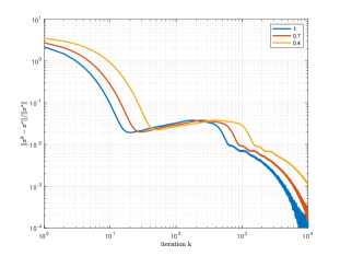
Figure 1: Normalized distance from the GNE.

VI Conclusion

The preconditioned forward–backward operator splitting is applicable to stochastic generalized Nash equilibrium problems to design distributed equilibrium seeking algorithms. Since the expected value is hard to compute in general, the sample average approximation can be used to ensure convergence almost surely. Our simulations show that the damping step may be unnecessary for convergence. We will investigate this case as future research.

References

- [1] F. Facchinei and C. Kanzow, “Generalized Nash equilibrium problems,” Annals of Operations Research, vol. 175, no. 1, pp. 177–211, 2010.
- [2] F. Facchinei and J.-S. Pang, Finite-dimensional variational inequalities and complementarity problems. Springer Science & Business Media, 2007.
- [3] L. Pavel, “An extension of duality to a game-theoretic framework,” Automatica, vol. 43, no. 2, pp. 226–237, 2007.
- [4] A. A. Kulkarni and U. V. Shanbhag, “On the variational equilibrium as a refinement of the generalized Nash equilibrium,” Automatica, vol. 48, no. 1, pp. 45–55, 2012.
- [5] G. Belgioioso and S. Grammatico, “Projected-gradient algorithms for generalized equilibrium seeking in aggregative games are preconditioned forward-backward methods,” in 2018 European Control Conference (ECC). IEEE, 2018, pp. 2188–2193.
- [6] P. Yi and L. Pavel, “An operator splitting approach for distributed generalized Nash equilibria computation,” Automatica, vol. 102, pp. 111–121, 2019.
- [7] G. Belgioioso and S. Grammatico, “Semi-decentralized Nash equilibrium seeking in aggregative games with separable coupling constraints and non-differentiable cost functions,” IEEE control systems letters, vol. 1, no. 2, pp. 400–405, 2017.
- [8] H. H. Bauschke, P. L. Combettes et al., Convex analysis and monotone operator theory in Hilbert spaces. Springer, 2011, vol. 408.
- [9] C.-K. Yu, M. Van Der Schaar, and A. H. Sayed, “Distributed learning for stochastic generalized Nash equilibrium problems,” IEEE Transactions on Signal Processing, vol. 65, no. 15, pp. 3893–3908, 2017.
- [10] U. Ravat and U. V. Shanbhag, “On the characterization of solution sets of smooth and nonsmooth convex stochastic Nash games,” SIAM Journal on Optimization, vol. 21, no. 3, pp. 1168–1199, 2011.
- [11] H. Xu and D. Zhang, “Stochastic Nash equilibrium problems: sample average approximation and applications,” Computational Optimization and Applications, vol. 55, no. 3, pp. 597–645, 2013.
- [12] D. Watling, “User equilibrium traffic network assignment with stochastic travel times and late arrival penalty,” European Journal of Operational Research, vol. 175, no. 3, pp. 1539–1556, 2006.
- [13] R. Henrion and W. Römisch, “On m-stationary points for a stochastic equilibrium problem under equilibrium constraints in electricity spot market modeling,” Applications of Mathematics, vol. 52, no. 6, pp. 473–494, 2007.
- [14] V. DeMiguel and H. Xu, “A stochastic multiple-leader Stackelberg model: analysis, computation, and application,” Operations Research, vol. 57, no. 5, pp. 1220–1235, 2009.
- [15] I. Abada, S. Gabriel, V. Briat, and O. Massol, “A generalized Nash–Cournot model for the northwestern european natural gas markets with a fuel substitution demand function: The gammes model,” Networks and Spatial Economics, vol. 13, no. 1, pp. 1–42, 2013.
- [16] R. I. Bot, P. Mertikopoulos, M. Staudigl, and P. T. Vuong, “Forward-backward-forward methods with variance reduction for stochastic variational inequalities,” arXiv preprint arXiv:1902.03355, 2019.
- [17] A. Iusem, A. Jofré, R. I. Oliveira, and P. Thompson, “Extragradient method with variance reduction for stochastic variational inequalities,” SIAM Journal on Optimization, vol. 27, no. 2, pp. 686–724, 2017.
- [18] J. Koshal, A. Nedic, and U. V. Shanbhag, “Regularized iterative stochastic approximation methods for stochastic variational inequality problems,” IEEE Transactions on Automatic Control, vol. 58, no. 3, pp. 594–609, 2013.
- [19] F. Yousefian, A. Nedić, and U. V. Shanbhag, “On smoothing, regularization, and averaging in stochastic approximation methods for stochastic variational inequality problems,” Mathematical Programming, vol. 165, no. 1, pp. 391–431, 2017.
- [20] ——, “Optimal robust smoothing extragradient algorithms for stochastic variational inequality problems,” in 53rd IEEE Conference on Decision and Control. IEEE, 2014, pp. 5831–5836.
- [21] L. Rosasco, S. Villa, and B. C. Vũ, “Stochastic forward–backward splitting for monotone inclusions,” Journal of Optimization Theory and Applications, vol. 169, no. 2, pp. 388–406, 2016.
- [22] D. P. Palomar and Y. C. Eldar, Convex optimization in signal processing and communications. Cambridge university press, 2010.
- [23] F. Facchinei, A. Fischer, and V. Piccialli, “On generalized Nash games and variational inequalities,” Operations Research Letters, vol. 35, no. 2, pp. 159–164, 2007.
- [24] A. N. Iusem, A. Jofré, R. I. Oliveira, and P. Thompson, “Variance-based extragradient methods with line search for stochastic variational inequalities,” SIAM Journal on Optimization, vol. 29, no. 1, pp. 175–206, 2019.
- [25] A. Kannan and U. V. Shanbhag, “The pseudomonotone stochastic variational inequality problem: Analytical statements and stochastic extragradient schemes,” in 2014 American Control Conference. IEEE, 2014, pp. 2930–2935.