Overlay Indexes: Efficiently Supporting Aggregate Range Queries and Authenticated Data Structures in Off-the-Shelf Databases

Abstract

Commercial off-the-shelf DataBase Management Systems (DBMSes) are highly optimized to process a wide range of queries by means of carefully designed indexing and query planning. However, many aggregate range queries are usually performed by DBMSes using sequential scans, and certain needs, like storing Authenticated Data Structures (ADS), are not supported at all. Theoretically, these needs could be efficiently fulfilled adopting specific kinds of indexing, which however are normally ruled-out in DBMSes design.

We introduce the concept of overlay index: an index that is meant to be stored in a standard database, alongside regular data and managed by regular software, to complement DBMS capabilities. We show a data structure, that we call DB-tree, that realizes an overlay index to support a wide range of custom aggregate range queries as well as ADSes, efficiently. All DB-trees operations can be performed by executing a small number of queries to the DBMS, that can be issued in parallel in one or two query rounds, and involves a logarithmic amount of data. We experimentally evaluate the efficiency of DB-trees showing that our approach is effective, especially if data updates are limited.

Keywords. Database systems, Indexes, Tree data structures, Data security, Computational efficiency, Aggregated range queries, Authenticated data structures.

1 Introduction

In relational and NoSQL databases, the ability to obtain aggregate information from a (possibly large) set of “records” (tuples, documents, etc.) has always been an important feature. Usually, the set on which to apply an aggregation function (e.g., COUNT or SUM in SQL [20]) is identified by some form of record selection. In the simplest form, records that have one of their fields in a given range are selected and the aggregation function is applied on them. This kind of queries are usually referred to as aggregate range queries. Applications of aggregate range queries can be easily found in many data analytics activities related to business intelligence, market analysis, user profiling, IoT, etc. Further, this feature is one of the fundamental elements of a good system for big-data analytics. In many applications, the speed at which queries are fulfilled is often critical, possibly marking the distinction between a system that meets the user needs and one that does not. Typical examples are interactive visual systems, where users expect the system to respond in less than a second.

The vast majority of DataBase Management Systems (DBMSes) supports aggregate range queries to some extent. When data are large, aggregation performed by a complete scan of the selected data can be too costly to be viable. In theory, adopting proper data structures for indexing [16], it is possible to answer aggregate range queries in $O(\log n)$ time, where $n$ is the amount of selected records to be aggregated, for any selection range and for a quite large class of aggregation functions. The general idea behind those data structures is to store partial pre-computed aggregate values in each node of the index. In this way, it is possible to answer aggregate range queries on any range without actually scanning the data. Update operations on these data structures also take logarithmic time, allowing them to be used even when data is subject to updates.

However, in practice, indexes realized by many DBMSes are designed to support regular (non aggregated) queries. This is reflected in the limited advantage that regular indexes can provide to aggregate range queries. In particular, most DBMSes can exploit regular indexes only for aggregation based on MIN and MAX functions. Other typically DBMS-supported aggregation functions, like SUM, AVG, etc., usually require sequential scans. To speed up these sorts of queries, a typical trick is to keep data in main memory, which is costly and usually not possible for big-data applications.

In this paper, we introduce the concept of overlay index, which is a data structure that plays the role of an index but is explicitly stored in a database along with regular data. The logic to use an overlay index is not frozen in the DBMS but can be programmed and customized at the same level of the application logic, obtaining great flexibility. However, designing an overlay index rises specific challenges. In principle, any memory oriented data structure could be easily represented in a database. Nonetheless, operations on these data structures typically require traversing a logarithmic number of elements, each of them pointing to the next one, which is an inherently sequential task. While this is fast and acceptable in main memory, sequentially performing a logarithmic number of queries to a DBMS is extremely slow. In fact, each query encompasses client/server communication, usually involving the network and the operating system, which introduces a large cost that cannot be mitigated by the DBMS query planner. Further, performing queries sequentially prevents the exploitation of the capability of RAID arrays and DBMS clusters to fulfill many requests at the same time and of disk schedulers to optimize the order of disk access [56].

Our main contribution is a new data structure, called DB-tree, for the realization of an overlay index. DB-trees are meant to be stored and used in standard DBMSes to support custom aggregate range queries and possibly other needs, like, for example, data authentication by Authenticated Data Structures [55] (ADS). DB-trees are a sort of search trees whose balancing is obtained through randomization, as for skip lists [47]. In a DB-tree, query operations require only a constant number of range selections, that can be executed in parallel in a single round and that return a logarithmic amount of data. Updates, insertions and deletions, also involve a logarithmic amount of data and can be executed in at most two rounds. We formally describe all algorithms and prove their correctness and efficiency.

Additionally, we present experimental evidence of the efficiency of our approach, on two off-the-shelf DBMSes, by comparing the queries running times using DB-trees against the same operations performed with the only support of the DBMS. Experimental results show that the adoption of DB-trees brings a large gain for range queries, but they may introduce a non negligible overhead when data changes. We also discuss several applicative and architectural aspects as well as some variations of DB-trees.

This paper is structured as follows. In Section 2, we show the state of the art. In Section 3, we introduce the concept of overlay index and discuss several architectural aspects. DB-trees are introduced in Section 4 along with some formal theoretical results. Algorithms to query a DB-tree and perform insertions, deletions and updates are shown in Section 5. In Section 6, we show an experimental comparison between DB-trees and plain DBMS. In Section 7, we show how it is possible to use DB-trees to perform, efficiently, aggregate range queries grouped by values of a certain column. We also show an experimental comparison with other approaches. In Section 8, we show how DB-trees can be adapted to realize persistent ADSes. In Section 9, we discuss some architecture generalizations. In Section 10, we draw the conclusions.

2 State of the Art

In this section, we review the state of the art of technology and research about aggregate range queries optimization. We also review the state of the art about persistent representation of ADSes, which is a relevant application of the results of this paper.

Optimization of query processing in DBMSes is a very classic subject in database research, which historically also dealt with the optimization of aggregate queries (see for example [59]). Indexes are primary tools for the optimization of query execution. They are data structures internally used by DBMSes to speed up searches. They are persisted on disk in a DBMS proprietary format. Typical indexes realize some form of balanced search tree or hash table [16, 49]. Specific indexing techniques for uncertain data are also known, see for example [13, 3, 11, 12]. Some research effort was also dedicated to the creation of a general architecture for indexing, see, for example, [29, 33]. However, these results have been adopted only by specific DBMSes (see, for example, [4]). The query optimizer of DBMSes can take into account the presence of indexes in the planning phase if this is deemed favorable. In a typical DBMS, the creation of an index is asked by the database administrator, or the application developer, using proper constructs (available for example in SQL). The decisions about indexes creation is usually based on the foreseen frequencies of the queries, the involved data size, and execution time constraints. Several works deal with the possibility for a DBMS to self tune and to choose right indexes (see, for example, [9, 34]). Usually, there is no way for the user of the DBMS to access an index directly or to create indexes that are different from the ones the DBMS is designed to support. A notable exception to this is the PostgreSQL DBMS that provides some flexibility [1].

Concerning aggregate range queries, in common DBMSes, regular indexing is usually only effective for some aggregate functions, like MIN and MAX. Sometimes, certain index usages can provide a great speed-up for aggregate range queries due to the fact that putting certain data in the index may avoid random disk access and/or most processing could occur in-memory [48]. The current DBMS technology and the SQL standard do not allow the user to specify custom indexes to obtain logarithmic time execution of aggregate range queries, even for SQL-supported aggregation functions for which this would be theoretically possible.

A wide variety of techniques was proposed to optimize the execution of aggregate range queries in DBMSes. A whole class of proposals deal with materialized views (see for example [28, 23, 27, 53, 40]). These techniques require the DBMS to keep the results of certain queries stored and up-to-date. These can be used to simplify the execution of certain aggregate queries and are especially effective when data is not frequently updated.

A largely investigated approach is called Approximate Query Processing (AQP), which aims at gaining efficiency while reducing the precision of query results. A survey of the achievements in this area is provided in [37]. This approach is relevant especially when data are large. An approximate approach targeted to big-data environments is proposed in [62]. A method to perform approximate queries on granulated data summaries of large datasets is shown in [52]. Approximated techniques are now available on some widely used systems [54, 8]. The VerdictDB [45] system provides a handy way to support AQP for SQL-based systems by adding a query/result-rewriting middle layer between the client and the DBMS.

A context in which aggregation speed is very relevant is in On-Line Analytical Processing (OLAP) systems (see, for example, [30, 26]). Several works deal with fast methods to obtain approximated results [51, 18, 2] for OLAP systems. In this field, specific indexing techniques may be adopted [50]. Specific data structures were proposed to support aggregated range queries, like for example aR-trees [44] for spatial OLAP systems. The work in [38] surveys several aggregation techniques targeted to the storage of spatiotemporal data.

To support strict time bounds, specific techniques for in-memory databases exist [10].

As will be clear in the following, one of the applications of our results is to support Authenticated Data Structures (ADS) (see Section 8). ADSes are useful when we need a cryptographic proof that the result of a query is coherent with a certain version of the dataset and that version is succinctly known to the client by a cryptographic hash that the client trusts. The first ADS was proposed by Merkle [39]. Merkle trees are balanced search trees in which each node contains a cryptographic hash of its children and, recursively, of the whole subtree. The work in [46] shows how to arbitrarily scale the throughput of an ADS-based system in a cloud setting with an arbitrarily large number of clients. ADSes are especially desirable in the context of outsourced databases. The work in [35] studies data structures to realize authenticated versions of B-trees to authenticate queries. This proposal is meant to be used in DBMSes as an internal indexing structure. Other works tried to represent ADSes in the database itself. Several general-purpose techniques to represent a tree are presented in [7]. The problem of representing an authenticated skip list [55] in a relational table was investigated in [19]. They propose the use of nested sets to perform queries in one query round. An efficient use of this approach to compute authenticated replies for a wide class of SQL queries is provided in [42]. Nested sets represents nodes of trees as intervals bounded by integers and a parent-child relation is represented as a containment relation between two intervals. Unfortunately, nested sets cannot be updated efficiently. In [58], several variations of nested sets are described, varying the way in which intervals bounds are represented. These methods are based on numerical representations of rational numbers and are limited by precision problems.

3 Overlay Indexes

In this section, we discuss the rationale for introducing overlay indexes, the applicative contexts where overlay indexes can be fruitfully applied and discuss some architectural aspects. This discussion is largely independent from the DB-tree data structure, which we propose as one form of realization of overlay indexes, described in Section 4.

In the following, when we refer to a query, we may intend either a proper data-reading query or a generic statement, which can also change the data. The distinction should be clear form the context.

Figure 1: A schematic architecture for the adoption of overlay indexes. Thick arrows shows the data path when overlay logic is realized client-side. Dotted arrows shows data path when overlay logic is realized by stored procedures in the DBMS.

In Figure 1, we show a schematic architecture for the adoption of overlay indexes. We suppose to have a client and a DBMS connected by a connection. In our scheme, the client contains the application logic and performs queries to the DBMS through the connection. Note that, we use this scheme in the following discussion but we do not intend to restrict the use of overlay indexes to this simple architecture. For example, the client may be the middle tier server that performs DBMS queries on behalf of user clients, the storage of the DBMS may be located in a cloud, the client may be on the same machine of the DBMS and the connection may be just inter-process communication, and so on. The protocol used to perform queries to the DBMS is a standard one (e.g., SQL or one of the many NoSQL query languages). Additional requirements on features supported by the DBMS depend on the way overlay indexes are realized. We provide these details for DB-trees in Section 4.2.

3.1 Applicative contexts

The applicative contexts where we believe overlay indexes may turn out to be of great help are those where (1) the application performs both updates (possibly comprising insertion and deletion) and reads on the database, (2) some read operations have strong efficiency requirements, like, for example, in interactive applications, (3) the amount of data is so large that in-memory solutions cannot be applied and, hence, the efficiency of those read operations can only be obtained by adopting indexes, and (4) the DBMS does not support the right indexing for those read operations. For example, an application might need to provide the sum of a column for those tuples having the value of their key contained in a certain range, which depends on (unpredictable) user requests, or might need to provide a cryptographic hash of the whole table to the client for security purposes. The first case, is often inefficiently supported and often efficiency is obtained not by proper indexing but by keeping data in main memory. The second case is usually not supported by DBMSes. Clearly, in the above described conditions, approximate query processing could be adopted. However, in certain situations approximation is not desirable or is ruled-out by the nature of the aggregation function, as for the cryptographic hash case.

3.2 Rationale

Clearly, the introduction of an overlay index has some performance overhead when data are updated, as any indexing approach has, but can be the only viable approach for certain non-supported aggregation functions or can dramatically reduce the time taken to reply to certain queries for which specific indexing is not available from the DBMS. For example, in the cases where the DBMS cannot use indexes, an aggregated query may run in $O(r)$ where $r$ is the number of elements in the range selected by the query. This is essentially due to the fact that the DBMS has no better strategy than sequentially scan the result of the selection. For an overlay index realized as a DB-tree (see Section 4), both queries and updates take $O(\log r)$. The speed-up obtained for the aggregate range queries may be huge, if $r$ is even moderately large, while paying a logarithmic slow-down on the update side is usually affordable, especially if data are rarely updated (see also Section 6).

3.3 Architectural Aspects

We refer to Figure 1. Realizing an overlay index requires to introduce (i) one or more specific table(s) into the database, which we call overlay table(s), alongside the regular data, with the purpose to store the overlay index, and (ii) a (possibly only conceptual) middle layer, which we call overlay logic, that is in charge of keeping overlay tables up-to-date with the data and to fulfill the specific queries the overlay index was introduced for.

We observe that the overlay logic can be naturally designed as a real middle layer, which should (1) take an original query performed by the client, for example expressed in plain or augmented SQL language, (2) produce appropriate actual queries that act upon regular tables and/or overlay tables and submit them to the DBMS, (3) get their results from the DBMS, and (4) compose and interpret the results to reply to the original query of the client. This is the approach taken by VerdictDB [45] for approximate processing of aggregated range queries. Since we aim at proving the soundness and the practicality of the overlay index approach, the construction of such a middle layer for overlay indexes is out of the scope of this paper.

A simpler approach is to have a library that is only in charge to change or query overlay tables. In this case, it is responsibility of the application to call this library to change an overlay table every time the corresponding regular data table is changed. Special care should be taken to keep consistency between the two. For example, the whole update (of data and overlay tables) should be performed within a transaction. In certain situations, it may be convenient to keep all the data within the index itself without having a distinct regular data table. This is the approach that we adopted for the experiments described in Section 6.

When designing a data structure for an overlay index, the time complexity of its operations is clearly a major concern. However, we should also take into account its efficiency in terms of data transferred for each operation, and also how this transfer is performed. In fact, to perform a query on an overlay index, it is likely that several actual queries to the DBMS should be performed. It is important that these queries could be done in parallel. A round is a set of actual queries that can be performed in parallel to the DBMS. We assume actual queries to be submitted to the DBMS at the same instant. The duration of a round is the time elapsed from queries submission to the end of the longest one. Round duration is composed of the execution time (on the DBMS) of the longest query and the communication latencies in both directions. A poor implementation may require the original query to take several rounds to be accomplished, possibly consisting of only one actual query each. For example, a plain porting of any balanced data structure (like, for example, AVL-trees, skip lists, or B-trees) to use a DBMS as storage would take $O(\log n)$ rounds for their operations, where $n$ is the number of elements in the data structure. This means that in the overall time to execute the original query, we should sum up the time spent by $O(\log n)$ actual queries for both communication and execution on the DBMS. As already mentioned, highly parallel systems (like RAID arrays) may greatly reduce the overall response time if the tasks they have to perform (i.e., sectors to be read or written) are all known in advance. In fact, they can usually execute many tasks concurrently making a much better use of resources and obtaining a much smaller execution time, overall. Even when a single hard drive is used, it is useful to know all the tasks in advance since disk schedulers reorder all the tasks they know so that they are fulfilled in a single sweep of the head of the hard drive [56] to reduce the time spent for seeking the correct tracks. Some studies show how disk schedulers are relevant also when solid state drives or virtualization is adopted [5, 32, 60].

To improve performances, the overlay logic may realize some form of caching by keeping part of the overlay table in the memory of the client. While this may speed up some queries, it introduces a cache consistency problem, if more clients are present. For data-changing queries, it is likely that the overlay logic needs to know beforehand the part of the overlay table that is going to be modified, before submitting the changes to the DBMS (this is the case for DB-trees, described in Section 4). The obvious approach is to perform changes in (at least) two rounds. The first (read round), to retrieve the part of the overlay table that is involved in the change and, the second (update round), to actually perform the change. The introduction of caching may help in reducing the amount of data transferred from the database in the read round. However, since the data needed for the change depends on the request performed by the user, caching is unlikely to make the read round unnecessary, unless the application always updates the same set of data. A particular case is the insertion of a large quantity of data (also called batch insert in technical DBMS literature). In this case, many insertions may be cumulated in cache and written in one round, possibly using batch insert support from the DBMS itself. We consider all aspects introduced by caching to be outside of the scope of this paper. In the realization adopted for the experimentation of Section 6, we do not adopt any form of caching and we have only one client.

It is worth mentioning that overlay logic may also be realized exploiting programmability facilities of certain DBMSes, usually called stored procedures. In this case, the impact of communication between the overlay logic and the DBMS would be negligible. This has two notable effects: (1) the inefficiency of data-changing operations due to the need of two query rounds is mitigated and (2) the adoption of a realization that performs in many rounds (e.g., logarithmic in the data size) becomes more affordable. Anyway, having many sequential query rounds still makes a poor use of RAID arrays, DBMS clusters, and disk schedulers. Hence, also in this setting, it is advisable to adopt special data structures that limit the number of query rounds, like DB-trees. We note that stored procedures are proprietary features of DBMSes, hence, exploiting them links overlay logic to a specific DBMS technology. Further, not all DBMSes support them, especially in the NoSQL world.

4 The DB-Tree Data Structure

In this section, we describe the DB-tree data structure, which we propose to realize an overlay index. We first describe it intuitively. Then, we provide a formal description of the data structure with its invariants. Finally, we describe its fundamental properties.

4.1 Intuitive Description

A DB-tree stores key-value pairs ordered by key. To simplify the description we assume that keys are unique and both keys and values have bounded length. A DB-tree is a randomized data structure that shares certain features with skip lists [47] and B-trees [15], which are widely used data structures to store key-value pairs, in their order. We start by recalling skip lists, which are conceptually simpler than DB-trees, and then we show how DB-trees derive from them. A formal description of DB-trees is provided in Section 4.2.

Figure 2: An example of a skip list. For each element, only the key is shown. Level 0 also stores values, not shown.

A skip list is made of a number of linked lists. An example is shown in Figure 2, where linked lists are drawn horizontally. Each element of those linked lists stores a key and each list is ordered. Each list is a level that is denoted by a number. Level zero contains all the keys and it is the only level that also stores values. Higher levels are progressively decimated, that is, each level above zero contains only a fraction of the keys of the level below. In this way, each key $k$ is associated with a tower of elements up to level $l(k)$, called height of the tower. For the example of Figure 2, we have $l(10)=0$ and $l(11)=3$. Beside regular pointers of linked lists, in skip lists, elements have also pointers that vertically link elements of the same tower.

Algorithm 1 Extraction of a random level.

1:A random level for a skip list or a DB-tree.

2: $\triangleright$ We denote by RandomChoice a random value in $\{\mbox{GO-UP},\mbox{STOP}\}$, where GO-UP is extracted with probability $p$ and STOP with probability $1-p$.

3:$l\leftarrow 0$

4:while  RandomChoice is GO-UP  do

5:     $l\leftarrow l+1$

6:end while

7:return $l$

In traditional skip lists, when $k$ is inserted, $l(k)$ is randomly selected using the approach described in Algorithm 1. We assume to have a random generator with two possible outcomes: GO-UP, with probability $p$, and STOP, with probability $1-p$. Initially, $l(k)$ is set to zero. We iteratively produce a random outcome and increase $l(k)$ each time we obtain GO-UP. The procedure ends when we obtain the first STOP. In this way, each level contains a fraction $p$ of the elements of the previous level. A typical value for $p$ is $1/2$. In a skip list, the search of a key $k$ proceeds as follows. First, we linearly search the highest level for the largest key less than or equal to $k$. If we have not found $k$ yet, we traverse the tower link descending of one level and start to search again until we either find $k$ (success) or reach level zero and a key greater than $k$. This procedure takes $O(\log n)$, where $n$ is the number of keys in the skip list. Deletion and insertion can be also performed in $O(\log n)$ (further details can be found in [47]).

Skip lists are regarded as efficient and easy-to-implement data structures, since they do not need any complex re-balancing. However, they are meant to be stored in memory, where traversing pointers is fast. An attempt to represent a skip list in databases was made in [19], resulting in operations taking $O(\log n)$ query rounds, since the execution of each round depends on the result of the previous one.

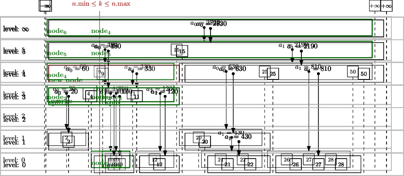
Figure 3: A DB-tree corresponding to the skip list shown in Figure 2 for the SUM aggregation function. For simplicity, we do not show values. In this and in the following examples, for each key $k$ the corresponding value is intended to be $v=10k$.

DB-trees can be interpreted, and intuitively explained, as a clever way of grouping elements of a corresponding skip list so that update and query operations can be performed in only one or two query rounds. The DB-tree corresponding to the skip list shown in Figure 2 is shown in Figure 3. To simplify the picture, in this and in the following examples, we show only keys and omit values, implicitly intending (only for the purpose of the examples) that for each $k$ the corresponding value $v$ is derived by $k$ so that $v=10k$. We construct a DB-tree starting from a skip list as follows. Levels of the DB-tree are in one-to-one correspondence with levels of the skip list. Only the elements at the top of each skip list tower are represented in the DB-tree and grouped into nodes. Nodes are associated with levels. Each node spans consecutive keys of its level, but it cannot span keys having, in between, others contained in some level above. In other words, nodes at level $l$ only contains keys $k$ such that $l(k)=l$. Each key at level above $l$ separates nodes at level $l$ and below. In Figure 3, this separation is represented by vertical dashed lines. The number of keys associated with a node is not fixed. Consider two adjacent, and not consecutive, keys in a node. The missing keys in that level are represented by nodes at inferior levels, which are children or descendants of that node.

Since we intend to use DB-trees to support aggregate range queries, we store in each node the aggregate values of the key-value pairs that are between two adjacent keys in the node, which are indeed explicitly contained in its descendants. We have one aggregate value for each child and the sequence of keys of a node is interleaved with the aggregate values related to children. An aggregate value is omitted if the corresponding child is not present. In the example of Figure 3, aggregate values are shown in the nodes interleaved with keys. We recall that, for the sole purposes of this example, values $v$ are derived from the corresponding $k$ ($v=10k$).

To realize a DB-tree, the overlay logic (see Section 3) stores its data in a single overlay table $T$. We use the relational DBMS jargon just for clarity, but we do not restrict the kind of the underlying DBMS to this class. The value associated with each key may be stored in $T$ itself, if the application does not need to perform other queries that are unrelated with the DB-tree. Otherwise, a regular table $D$ should be present, and $T$ is treated as an index that should be kept up-to-date with $D$. In the following, we consider only table $T$, intending that the shown results can be applied also if a corresponding $D$ is present. In the rest of the paper, we use the symbol $T$ to denote also an abstract DB-tree and we denote by $|T|$ the number of keys it contains.

4.2 Formal Description

A DB-tree contains key-value pairs, where keys are non-null, distinct, and inherently ordered, and values are from a set $V$. We intend to support, efficiently, arbitrary aggregate range queries. An aggregate range query performs aggregation on values related to keys within a range that is chosen by the user and it is not known in advance. We assume that the kinds of aggregation queries to support are based on a decomposable aggregation function A decomposable aggregation function $\alpha:V^{n}\rightarrow C$ is obtained by composing a triple of functions $\langle f,g,h\rangle$ defined as follows.

• $f:A\times A\rightarrow A$ is associative, that is $f(a,b,c)=f(f(a,b),c)=f(a,f(b,c))$, and there exists an identity element denoted by $1_{A}$, that is for any $x\in A:f(1_{A},x)=f(x,1_{A})=x$. The associativity of $f(a,b)$ allows us to write $f(a_{1},\dots,a_{n})$, since the grouping according to which $f$ is applied is irrelevant for the final result.

• $g:V\rightarrow A$.

• $h:A\rightarrow C$.

We define $\alpha(v_{1},\dots,v_{n})=h(f(g(v_{1}),\dots,g(v_{n})))$. We call $f$ the core aggregation function. In the following, by aggregation function, we refer to either the single core aggregation function $f$ or the whole decomposable aggregation function (i.e., the triple). The actual meaning should be clear from the context. Depending on $g$, $V$ may or may not comprehend the null value. In the following, results of evaluation of $f(\cdot)$ are called aggregate values.

This model can support many practical aggregation functions, like, count, sum, average, variance, top-$n$, etc., which are referred to as distributive and algebraic aggregation functions in literature [25]. For example, we can support top-2 (giving the first and second maximum) with the following definitions.

• $A=\{V,\bot\}\times\{V,\bot\}$, where we intend that the first element of each pair is the maximum, the second is the second maximum, $\bot$ means undefined, and $\bot$ is less than any element in $V$,

• $g(v)=(v,\bot)$,

• $h(x)=x$,

• $f((v_{1},v_{2}),(v_{3},v_{4}))=(m_{1},m_{2})$ where $m_{1}=\max\{v_{1},v_{3}\}$ and $m_{2}$ is the second maximum in $U=\{v_{1},v_{2},v_{3},v_{4}\}$, that is $m_{2}=\max(U-\{m_{1}\})$, and

• the identity element is $(\bot,\bot)$.

The above definitions can be easily generalized to support top-$n$. Our model does not directly support so-called holistic aggregation functions. In this kind of aggregation functions, there is no constant bound on the size of the storage needed to describe a sub-aggregate [25]. For this reason, they are commonly recognized as hard to optimize (see for example [61, 36, 14]). Examples of this kind of aggregation functions are median, n-th percentile, and mode.

We are now ready to formally describe the DB-tree data structure. DB-trees support any aggregation function that fits the definition of decomposable aggregation function stated above. We assume that the aggregation function to be supported is known before the creation of the DB-tree, or at least $g$ and $f$ are known.

A DB-tree, keeps certain aggregate values ready to be used to compute aggregate range queries on any range, quickly. Its distinguishing feature with respect to other results known in literature is that it is intended to be efficiently stored and managed in databases. While typical research works in this area show data structures whose elements are accessed by memory pointers (for in-memory data structures) or by block addressing (for disk/filesystem based data structures), the primary mean to access the elements of a DB-tree is by range selection queries provided by the DBMS itself.

We do not restrict the kind of underlying database that can be used to store a DB-tree. However, for simplicity, we describe our model using terminology taken from relational databases. We only require the underlying database to have (i) the ability to perform range selection on several columns, efficiently, which is usually the case when proper indexes are defined on the relevant columns, and (ii) the ability to get, efficiently, the tuple containing the maximum (or minimum) value for a certain column among the selected tuples.

A DB-tree $T$ contains a sequence of key-value pairs, ordered according to their keys. A DB-tree is logically made of nodes forming a rooted tree. Each node $n$ of a DB-tree stands for a subsequence of contiguous key-value pairs of $T$, denoted by $\mathrm{standsfor}(n)$.

A node $n$ is associated with an open interval $(n.\mathrm{min},n.\mathrm{max})$ called range, denoted $\mathrm{range}(n)$, where $n.\mathrm{min}$ and $n.\mathrm{max}$ are either keys in $T$ or can assume values $-\infty$ or $+\infty$. In any case, it should hold that $n.\mathrm{min}<n.\mathrm{max}$. A node $n$ stands for the subsequence of key-value pairs in $T$ whose keys are strictly contained in $\mathrm{range}(n)$. In other words, $n.\mathrm{min}$ is the key in $T$ right before $\mathrm{standsfor}(n)$, or $-\infty$ if it does not exist, and $n.\mathrm{max}$ is the key in $T$ right after $\mathrm{standsfor}(n)$, or $+\infty$ if it does not exist.

A node $n$ explicitly contains only some key-value pairs among those of $\mathrm{standsfor}(n)$. The key-value pairs that are explicitly contained in $n$, do not need to be necessarily contiguous in $\mathrm{standsfor}(n)$. Those that are not explicitly contained in $n$ are contained in nodes that are descendants of $n$. The root of $T$ stands for the whole sequence contained in $T$ and has range $(-\infty,+\infty)$. A node $n$ is associated with its aggregate sequence, which is derived from $\mathrm{standsfor}(n)$ by substituting the key-value pairs that are not explicitly contained in $n$ with the corresponding aggregate values. More formally, the aggregate sequence for a node $n$ is $a_{0},p_{1},a_{1},\dots,a_{m-1},p_{m},a_{m}$, denoted $n.\mathrm{aseq}$, where $p_{i}$’s are key-value pairs $\langle k_{i},v_{i}\rangle$, $m$ is the number of keys in $n.\mathrm{aseq}$, and $a_{i}$’s are aggregate values (note that subscripts indicate positions of key-value pairs within $n.\mathrm{aseq}$ and not within the whole sequence in $T$). We say that $n$ contains a key $k$ when $k$ is in $n.\mathrm{aseq}$. Some of the aggregate values in $n.\mathrm{aseq}$ may be missing, as it is explained in the following. It is worth noting that, if $k_{1},k_{2},\dots,k_{m}$ are contained in $n$, it should hold that $n.\mathrm{min}<k_{1}<k_{2}<\dots<k_{m}<n.\mathrm{max}$. The number $m$ of key-value pairs contained in a node is not the same for all nodes and may vary when the DB-tree is updated. The value $m$ related to a node $n$ is denoted $n.m$.

For each node $n$, the children of $n$ are in one-to-one correspondence with aggregate values in $n.\mathrm{aseq}$. We denote $n_{i}$ the child of $n$ associated with aggregate value $a_{i}$ in $n.\mathrm{aseq}$. Keys in $n.\mathrm{aseq}$ impose limits on the keys contained in the children. Namely, $n_{i}.\mathrm{min}=k_{i}$ and $n_{i}.\mathrm{max}=k_{i+1}$, but for $n_{0}$, for which $n_{0}.\mathrm{min}=n.\mathrm{min}$, and $n_{m}$, for which $n_{m}.\mathrm{max}=n.\mathrm{max}$, respectively. If $k_{i}$ and $k_{i+1}$ are consecutive in $\mathrm{standsfor}(n)$, the $i$-th aggregate value in $n.\mathrm{aseq}$ is missing, and the corresponding child is also missing. If an aggregate value and its corresponding child are not missing we say that they are present. The (present) aggregate value $a_{i}$ is the value of the core aggregation function on $\mathrm{standsfor}(n_{i})$. In practice, exploiting the associative property of $f(\cdot)$, we compute $a_{i}$ on the basis of $n_{i}.\mathrm{aseq}$. Let $n.\mathrm{aseq}=a_{0},\langle k_{1},v_{1}\rangle,a_{1},\dots,a_{m-1},\langle k_{m},v_{m}\rangle,a_{m}$, we define $f(n)=f(a_{0},g(v_{1}),a_{1},\dots,a_{m-1},g(v_{m}),a_{m})$, where we intend that any missing aggregate value should be omitted from the list of the arguments of $f(\cdot)$. Hence, we can write $a_{i}=f(n_{i})$.

Each node $n$ has a level denoted $n.\mathrm{level}\geq 0$, which is $\infty$ for the root. The children of $n$ have levels that are strictly lower than $n.\mathrm{level}$. We say that a node $n^{\prime}$ is above (below) $n$ if level of $n^{\prime}$ is greater (lower) than the level of $n$.

When a key $k$ is inserted into a DB-tree, it is associated with a randomly selected level obtained using Algorithm 1. The level of $k$ is denoted $l(k)$. Key $k$ is then inserted in a node at that level.

4.3 Summary of Invariants

We now formally summarize the invariants that must hold for each node $n$ in a DB-tree $T$. In the following $m=n.m$, $l=n.\mathrm{level}$, $n.\mathrm{aseq}=a_{0},\langle k_{1},v_{1}\rangle,a_{1},\dots,a_{m-1},\langle k_{m},v_{m}\rangle,a_{m}$ where some $a_{i}$ are possibly missing, as explained above. Children of $n$ are denoted $n_{0},\dots,n_{m}$ and some of them may be possibly missing.

1. If $n$ is the root of $T$, $n.\mathrm{min}=-\infty$, $n.\mathrm{max}=+\infty$, $n.\mathrm{level}=+\infty$. If $T$ is empty, $n.m=\bot$, $n.\mathrm{aseq}$ is an empty sequence and $n$ has no children. If $T$ is not empty, $n.m=0$, $n.\mathrm{aseq}=a_{0}$ and $n$ has one child.

2. If $n$ is not root, $n.m>0$ and
   $n.\mathrm{min}<k_{1}<k_{2}<\dots<k_{m}<n.\mathrm{max}$.

3. If $n_{i}$ (with $0\leq i\leq m$) is present, $n_{i}.\mbox{level}<n.\mbox{level}$,
   $n_{i}.\mathrm{min}=\begin{cases}n.\mathrm{min}&\text{if }i=0\\ k_{i}&\text{otherwise}\end{cases}$
   and
   $n_{i}.\mathrm{max}=\begin{cases}n.\mathrm{max}&\text{if }i=m\\ k_{i+1}&\text{otherwise}\end{cases}$

4. for all $i=0,\dots,m$, $a_{i}$ is present iff $n_{i}$ is present and $a_{i}=f(n_{i})$

4.4 Fundamental Properties

In this section, we introduce some fundamental properties that are important for proving the efficiency of the algorithms described in Section 5.

The following property is a direct consequence of Invariants 2 and 3.

Property 1 (Range Monotonicity).

Given a node $n$ of a DB-tree and $n^{\prime}$ parent of $n$, $\mathrm{range}(n)\subseteq\mathrm{range}(n^{\prime})$.

Now we analyze the relationship among nodes and between nodes and keys. Let $n$ be a node that contains $k$. Key $k$ cannot be contained in a node that is above $n$, since for all nodes above $n$ (which have $k$ in their range) $k$ is represented by an aggregate value (see Invariants 4). Key $k$ cannot be contained in a node that is below $n$, since it does not exist any of those nodes whose range contains $k$ (see Invariants 3 plus the definition of $\mathrm{range}(\cdot)$ as an open interval). From the above considerations, the following properties hold.

Property 2 (Unique Containment).

A key $k$ contained in a DB-tree $T$ is contained in one and only one node of $T$.

Property 3 (Lowest Level).

The node that contains a key $k$ is the one with minimum level among those that have $k$ in their range.

Concerning space occupancy, we note that in a DB-tree, a node contains one or more key-value pairs and each of them is contained in at most one node. This means that nodes are at most as many as the key-value pairs stored in the DB-tree. Hence, the space occupancy for a DB-tree is $O(|T|)$, in the worst case. In Section 6, we also provide some details about space occupancy in practice.

To reason about the size of the data that are transferred between the overlay logic and the DBMS, it is useful to state the following property.

Property 4 (Expected Node Size).

The expected number of keys that are contained in each node of a DB-tree is the same for all nodes.

This property can be derived from a consideration on the homogeneity of the levels. The number of keys contained in a node at level $i$ depends from the probability $p$ with which a key has level greater than $i$. In fact, these are the keys that partition keys of level $i$ into distinct nodes. Since $p$ does not depends on $i$, this proves the property.

The following lemma states a fundamental result on which the efficiency of querying a DB-tree is based.

Lemma 1 (Expected maximum level).

Given a set of $r$ keys ${k_{1},\dots,k_{r}}$ contained in a DB-tree $T$, the expected value of $\max\{l(k_{1}),\dots,l(k_{r})\}$, where $l(k_{i})$ is the level of $k_{i}$, is $O(\log r)$.

In other words, considering $r$ keys, the expected value of the maximum of their levels is logarithmic in $r$. Note that, this result also holds for skip lists, but we were not able to find its proof in standard skip list literature. For example, in [47], the proposed method for dimensioning the number of levels of a skip list focuses on the level whose expected number of elements is $1/p$, which is $O(\log n)$ with $n$ the number of keys in the skip list. While this approach is viable for the maximum level, it cannot be applied when we should measure the number of levels spanned by a subset of the keys that are contained in a much larger skip list or DB-tree.

The probability that $r$ keys are all at levels less than or equal to $i$ is $(1-p^{i+1})^{r}$, since all random levels are independent. The probability that the maximum is at level $i$ is $(1-p^{i+1})^{r}-(1-p^{i})^{r}$, since this is the probability of having all keys below $i+1$ minus the probability that all of them are below $i$. Hence, the expected maximum level for $r$ keys can be expressed as $\sum_{i=0}^{\infty}{i\left((1-p^{i+1})^{r}-(1-p^{i})^{r}\right)}$, which can be rewritten as $\sum_{k=1}^{r}(-1)^{k-1}\binom{r}{k}\frac{p^{k}}{1-p^{k}}$ by expanding binomials powers, reordering, and solving the infinite sum. Sums similar to this are known to be quite subtle to deal with. Flajolet and Sedgewick have provided several examples of how to tackle this kinds of sums in [22] using a mathematical tool called “Nørlund–Rice integral”. The proof that the above sum is $O(\log r)$ can be found in [41].

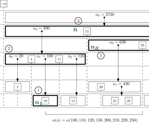
(a) The nodes contributing to the construction of the sequence $s$, i.e., in the set $N$, are highlighted with thick contours.

1. $n_{L}$: $s=[100]$

2. ancestor of $n_{L}$: $s=s\|[110,a_{2}]=[100,110,120]$

3. $\bar{n}$: $s=s\|[150]=[100,110,120,150]$

4. no nodes are between of $\bar{n}$ and $n_{R}$

5. $n_{R}$: $s=s\|[a_{0},250]=[100,110,120,150,630,250]$

(b) The steps for the construction of the sequence $s$ for the example. Sequences of values are shown within square brackets. Concatenation of sequences is denoted by $||$.

Figure 4: An example of construction of an aggregate range query according to the proof of Lemma 2. In this example, the query regards the sum of the values of the keys in the range from 10 to 25. The aggregation function is SUM and for each $k$ its value is $v=10k$.

The following lemma is relevant to understand the correctness of the query procedure that is algorithmically introduced in Section 5.

Lemma 2 (Aggregate Range Query Construction).

Given a sequence of keys $k_{1}<k_{2}<\dots<k_{r}$ contained in a DB-tree $T$ with their associated values $v_{1},\dots,v_{r}$, the aggregation function $\alpha(v_{1},v_{2},\dots,v_{r})$ can be computed from selected parts of the aggregate sequences of a set of nodes $N$ of $T$ containing

• the node that contains $k_{1}$, denoted $n_{L}$,

• the node that contains $k_{r}$, denoted $n_{R}$,

• the common ancestor of $n_{L}$ and $n_{R}$ with minimum level, denoted $\bar{n}$,

• the ancestors of $n_{L}$ and $n_{R}$ up to $\bar{n}$.

Proof.

We build a sequence $s$, that contains some of the values in $\{v_{1},v_{2},\dots,v_{r}\}$ and the missed values are substituted by aggregate values form nodes of $N$. We show that $\alpha(s)=\alpha(v_{1},v_{2},\dots,v_{r})$. We build $s$ from the aggregate sequences of nodes in $N$. Sequence $s$ is built from left to right. An example of the construction described in this proof is shown in Figure 4.

We start with $s$ containing, from $n_{L}.\mathrm{aseq}$, value $v_{1}$ associated with $k_{1}$ and all values (aggregated or not) at its right, in their order. We proceed by considering ancestors of $n_{L}$ in $N$ excluding $\bar{n}$, ordered by increasing level. For each of them, denoted by $n$, let $n^{\prime}$ be its descendant in $N$. We add to $s$, from $n.\mathrm{aseq}$, the value associated with $n^{\prime}.\mathrm{max}$, and all values (aggregated or not) at its right in their order. We do that, if $n^{\prime}.\mathrm{max}$ exists in $n.\mathrm{aseq}$, otherwise we skip to the next node. Let $n^{\prime}$ and $n^{\prime\prime}$ be the two descendants of $\bar{n}$, with $n^{\prime}.\mathrm{max}\leq n^{\prime\prime}.\mathrm{min}$. We add to $s$, from $\bar{n}.\mathrm{aseq}$, the value associated with $n^{\prime}.\mathrm{max}$ and all values (aggregated or not) at its right, in their order, up to the value associated with $n^{\prime\prime}.\mathrm{min}$ ($n^{\prime}.\mathrm{max}$ and $n^{\prime\prime}.\mathrm{min}$ exists in $\bar{n}.\mathrm{aseq}$ by construction of $\bar{n}$, $n^{\prime}$ and $n^{\prime\prime}$, and by Invariant 3). We continue by considering each ancestor $n$ of $n_{R}$ in $N$, excluding $\bar{n}$, ordered by decreasing level. Let $n^{\prime}$ be the descendant of $n$ in $N$. We add to $s$, from $n.\mathrm{aseq}$, all values (aggregated or not) starting from left up to the value associated with $n^{\prime}.\mathrm{min}$, in their order. We do that, if it exists in $n.\mathrm{aseq}$, otherwise we skip to the next node. Finally, we add to $s$, from $n_{R}.\mathrm{aseq}$, all values (aggregated or not) starting from left up to value $v_{r}$ associated with $k_{r}$, in their order. To prove that $\alpha(s)=h(f(s))=h(f(g(v_{1}),g(v_{2}),\dots,g(v_{r}))=\alpha(v_{1},v_{2},\dots,v_{r})$, we inductively apply Invariant 4, to $f(s)$. This allows us to express each aggregate value in $s$ as application of $f(\cdot)$ to the aggregate sequence of the corresponding child. The associative property of $f(\cdot)$ ensures that the aggregate value remains the same. ∎

Lemma 2 states that it is possible to answer to an aggregate range query considering only certain parts of the aggregate sequences of a small set of nodes $N$. We now estimates the size of $N$. The following result relates this size to the results stated by Lemma 1.

Lemma 3.

Given a sequence of keys $k_{1}<k_{2}<\dots<k_{r}$ contained in a DB-tree $T$, let $n_{L}$ and $n_{R}$ be the nodes containing $k_{1}$ and $k_{r}$, respectively, and call $\bar{n}$ their common ancestor with minimum level, the level of $\bar{n}$ is given by the maximum of the levels $l(k_{1}),l(k_{2}),\dots,l(k_{r})$.

The above lemma is easily proven considering the construction used for proving Lemma 2. Each of the keys $k_{1},k_{2},\dots,k_{r}$ is either contained in one of the nodes in $N$ or in one of its descendants. Note that, at least one of the keys is contained in $\bar{n}$, which is above of all other nodes in $N$. This means the $\bar{n}.\mathrm{level}=\max\{l(k_{1}),l(k_{2}),\dots,l(k_{r})\}$.

Lemma 4 (Aggregate Range Query Size).

Given a DB-tree $T$ and $k^{\prime}<k^{\prime\prime}$ two keys contained in $T$, such that $[k^{\prime},k^{\prime\prime}]$ contains $r$ keys in $T$, the aggregate range query on $[k^{\prime},k^{\prime\prime}]$ can be answered considering expected $O(\log r)$ values spread on expected $O(\log r)$ nodes.

Proof.

The proof of Lemma 2 constructs an aggregated sequence $s$ out of the aggregates sequences of nodes in $N$ which is made of two descending paths with a common ancestor $\bar{n}$. Lemma 3 states that the level of $\bar{n}$ is the maximum of the levels assigned to keys in $[k_{1},k_{r}]$, with $k^{\prime}\leq k_{1}$ and $k_{r}\leq k^{\prime\prime}$. Lemma 1 states that this maximum is expected to be $O(\log r)$. Since each of the two ascending paths constructed in the proof of Lemma 2 contains at most one node for each level, the maximum number of nodes needed to answer to an aggregate range query is expected $O(\log r)$. This proves the statement about the expected number of nodes involved in the query. Since the size of each node has constant expected size (Property 4), it can provide only an expected constant number of values. Hence, also the number of values are expected $O(\log r)$. ∎

5 DB-Tree Algorithms

Algorithm 2 Algorithm for performing an aggregate range query on a DB-tree.

1:Two keys $k^{\prime}$ and $k^{\prime\prime}$ (with $k^{\prime}<k^{\prime\prime}$ ) and a DB-tree $T$.

2:$\alpha(v_{1},\dots,v_{r})$ where $\langle k_{1},v_{1}\rangle,\dots,\langle k_{r},v_{r}\rangle$ and $k_{1},\dots,k_{r}$ are all the keys contained in $T$ within $k^{\prime}$ and $k^{\prime\prime}$, and $k^{\prime}\leq k_{1}<\dots<k_{r}\leq k^{\prime\prime}$.

3:$\triangleright$ Execute Lines 4-6 in one query round.

4:$L\leftarrow$ a sequence of nodes resulting from the selection from $T$ of all nodes $n$ such that $n.\mathrm{min}<k^{\prime}<n.\mathrm{max}\leq k^{\prime\prime}$ ordered by ascending level.

5:$R\leftarrow$ a sequence of nodes resulting from the selection from $T$ of all nodes $n$ such that $k^{\prime}\leq n.\mathrm{min}<k^{\prime\prime}<n.\mathrm{max}$ ordered by ascending level.

6:$\bar{n}\leftarrow$ the node $n$ in $T$ such that $n.\mathrm{min}<k^{\prime}<k^{\prime\prime}<n.\mathrm{max}$, with minimum level.

7:$a_{L}\leftarrow 1_{A}$, where $1_{A}$ is the identity element of $A$

8:for all  nodes $n$ in $L$ in ascending order  do

9:      $s\leftarrow\begin{cases}f(v_{i},a_{i},\dots,v_{m},a_{m}),\mbox{ where }k^{\prime}\leq k_{i},&\mbox{if there exists at least one }\langle k_{i},v_{i}\rangle\mbox{ with }k^{\prime}\leq k_{i}\\ 1_{A},&\mbox{otherwise}\end{cases}$

10:     $a_{L}\leftarrow f(a_{L},s)$

11:end for

12:$a_{R}\leftarrow 1_{A}$

13:for all  nodes $n$ in $R$ in ascending order  do

14:      $s\leftarrow\begin{cases}f(a_{0},v_{1},\dots a_{i-1},v_{i}),\mbox{ where }k_{i}\leq k^{\prime\prime},&\mbox{if there exists at least one }\langle k_{i},v_{i}\rangle\mbox{ with }k_{i}\leq k^{\prime\prime}\\ 1_{A},&\mbox{otherwise}\end{cases}$

15:     $a_{R}\leftarrow f(s,a_{R})$

16:end for

17:Let $\bar{n}.\mathrm{aseq}$ be $a_{0},\langle k_{1},v_{1}\rangle,a_{1},\dots,\langle k_{m},v_{m}\rangle,a_{m}$

18:$s\leftarrow f(v_{i},a_{i},\dots a_{j-1},v_{j})$ where $k_{i}$ is the lowest key such that $k^{\prime}\leq k_{i}$ and $k_{j}$ is the highest key such that $k_{j}\leq k^{\prime\prime}$.

19:return $f(a_{L},s,a_{R})$

In this section, we describe the algorithms to perform queries on a DB-tree and to modify its content. We also state their correctness and efficiency on the basis of the fundamental properties provided in Section 4.4. At the end of the section, we provide a comparison with similar data structures.

In the following, to simplify the description, we always assume $g(v)=v$ and $h(v)=v$ and never apply $g(\cdot)$ and $h(\cdot)$ explicitly. The adaption to the case of non-trivial $g(\cdot)$ and $h(\cdot)$ is straightforward.

When writing the algorithms, we denote by $a_{0},\langle k_{1},v_{1}\rangle,$ $a_{1},\dots,$ $\langle k_{m},v_{m}\rangle,a_{m}$ the aggregate sequence of a node $n$ containing $m$ keys. We use that notation implicitly meaning that some $a_{j}$ may be missing (see Section 4.2). For example, using that notation we includes sequences like $\langle k_{1},v_{1}\rangle,\langle k_{2},v_{2}\rangle,a_{2}$, for $m=2$, where $a_{0}$ and $a_{1}$ are missing. We also includes the special case in which $m=0$, where the sequence is only $a_{0}$. Analogously, we write $f(v_{i},a_{i},\dots,a_{j-1}v_{j})$, $f(a_{0},v_{1},\dots,a_{i-1}v_{i})$, and $f(v_{i},a_{i},\dots v_{m},a_{m})$ to aggregate a subsequence of an aggregate sequence of a node, again, implicitly meaning that some aggregate values may be missing.

5.1 Aggregate Range Query

The procedure to compute an aggregate range query is shown in Algorithm 2. Two keys $k^{\prime}$ and $k^{\prime\prime}$, not necessarily contained in DB-tree $T$, are provided as input. The algorithm computes the aggregate value for the values of all keys between $k^{\prime}$ and $k^{\prime\prime}$ in $T$. The procedure closely follows the proof of Lemma 2. Firstly, it retrieves the nodes cited in the statement of that lemma, plus some others that we will prove, are irrelevant. This is done in Lines 4-6. These queries can be performed in parallel in a single query round. The size of the data is $O(\log r)$ by Lemma 4, where $r\leq|T|$ is the number of keys between $k^{\prime}$ and $k^{\prime\prime}$. Hence, the following theorem about efficiency of Algorithm 2 holds.

Theorem 1 (Query Efficiency).

On a DB-tree $T$, an aggregate range query on a range containing $r$ keys in $T$ can be executed, by Algorithm 2, in only one query round and the expected size of the transferred data is $O(\log r)$.

Since Algorithm 2 processes each retrieved node a constant number of times, the execution of the part of the algorithm after data retrieval has expected time complexity $O(\log r)$.

We now focus on the correctness of Algorithm 2. Referring to the symbols introduced by the statement of Lemma 2, we consider $k_{1}$ as the lowest key in $T$ such that $k^{\prime}\leq k_{1}$ and $k_{r}$ as the highest key in $T$ such that $k_{r}\leq k^{\prime\prime}$. By construction, there is no other key between $k^{\prime}$ and $k_{1}$ and between $k_{r}$ and $k^{\prime\prime}$ in $T$.

We show that the set of nodes $N^{\prime}=L\cup R\cup\{\bar{n}\}$, selected by the algorithm, contains the set of nodes $N$ identified by the statement of Lemma 2. The correctness of Algorithm 2 will be given by the fact that the result of the aggregate value computed on both sets of nodes are equal.

Figure 5: An example in which Algorithm 2 selects more nodes than those considered in Lemma 2. The additionally selected nodes are evidenced with fat borders. See text for details.

We now analyze the differences between $N^{\prime}$ (of the algorithm) and $N$ (of the lemma). Refer to Figure 5 for an example. The algorithm selects a $n^{\prime}_{L}$ such that $n^{\prime}_{L}.\mathrm{min}<k^{\prime}<n^{\prime}_{L}.\mathrm{max}$, if $k_{1}<n^{\prime}_{L}.\mathrm{max}$ the node $n^{\prime}_{L}$ is equal to $n_{L}$ selected by the lemma, otherwise $n_{L}$ is an ancestor of $n^{\prime}_{L}$. Analogous reasoning can be done for $n^{\prime}_{R}$ and $n_{R}$. Figure 5 shows a case in which $n^{\prime}_{L}.\mathrm{max}=k_{1}$ and hence $n_{L}$ is an ancestor of $n^{\prime}_{L}$. In the same figure, $n^{\prime}_{R}.\mathrm{min}=k_{r-1}<k_{r}$ and hence $n^{\prime}_{R}=n_{R}$.

This means that $L$ and $R$ of the algorithm may additionally include descendants of $n_{L}$ and $n_{R}$ down to $n^{\prime}_{L}$ and $n^{\prime}_{R}$, respectively. The remaining part of $L$ ($R$) coincides with ancestors of $n_{L}$ ($n_{R}$), for both the algorithm and the lemma. We now show that $\bar{n}$ is the same for both the algorithm and the lemma. From the relationship $k^{\prime}\leq k_{1}<k_{r}\leq k^{\prime\prime}$, $\bar{n}$ in the algorithm might be an ancestor of $\bar{n}$ in the lemma, since the range of the first may only be larger than the range of the second. By Invariant 3, the range of a child is smaller only when there is a key in the parent that limits the range of the child, but this is not possible in our case, since no other key is present between $k^{\prime}$ and $k_{1}$ and/or between $k_{r}$ and $k^{\prime\prime}$, by construction. This means that $\bar{n}$ is the same for both the algorithm and the lemma.

We have just proven that $N^{\prime}$ can differ from $N$ only by some descendants of $n_{L}$ and $n_{R}$. Now, we prove that the contribution of those descendants to the overall aggregate value is null. Consider the relevant case $n^{\prime}_{L}\neq n_{L}$, we have that $k_{1}$ is contained in $n_{L}$ by construction, $k^{\prime}$ is contained in $\mathrm{range}(n^{\prime}_{L})$ by construction, no key is between $k^{\prime}$ and $k_{1}$ by construction. This implies that $n^{\prime}_{L}.\mbox{max}=k_{1}$ by Invariant 3 and that there is no key in $n^{\prime}_{L}.$aseq greater that $k^{\prime}$ to considered in the computation of the aggregate value (see Line 9). The same reasoning holds even if there are several nodes between $n^{\prime}_{L}$ and $n_{L}$. An analogous reasoning can be done about the contribution of nodes from $n^{\prime}_{R}$ up to and excluding $n_{R}$.

The above considerations together with the Lemma 2 prove the following theorem about the correctness of Algorithm 2.

Theorem 2 (Query Correctness).

An aggregate range query executed by Algorithm 2 on a DB-tree $T$ with range $[k^{\prime},k^{\prime\prime}]$ correctly returns $\alpha(v_{1},\dots,v_{r})$ where $v_{1},\dots,v_{r}$ are the values corresponding to all keys $k_{1},\dots,k_{r}$ in $T$ such that $k^{\prime}\leq k_{1}<\dots<k_{r}\leq k^{\prime\prime}$.

5.2 Update, Insertion and Deletion

Algorithm 3 This algorithm propagates the change of values of a certain node into the aggregate values in all its ancestors. It also inserts aggregate values that should be present in the aggregate sequence since the corresponding child is present. This algorithm is intended to be performed on a pool of nodes stored in main memory.

1:A sequence $U$ of nodes, in ascending order of level, representing an ascending path in a DB-tree. The first node of $U$ is denoted $\bar{n}$.

2:Aggregate values of nodes in $U$ above $n$ are updated to reflect the current state of $\bar{n}$.

3:$a\leftarrow f(\bar{n})$

4:$k\leftarrow$ any key contained in $\bar{n}$.

5:Remove $\bar{n}$ from $U$

6:for  each node $n$ in $U$ in ascending order of level do

7:     Let $a_{0},p_{1},a_{1},\dots,p_{m},a_{m}$ be $n.\mathrm{aseq}$ with $m=n.m$ and $p_{i}=\langle k_{i},v_{i}\rangle$ $\triangleright$ Some $a_{i}$’s might be missing.

8:     switch  do $\triangleright$ This switch can assigns a previously missing $a_{i}$ making it present.

9:         case  $m=0$

10:              $a_{0}\leftarrow a$          

11:         case  $k<k_{1}$

12:              $a_{0}\leftarrow a$          

13:         case  $k_{m}<k$

14:              $a_{m}\leftarrow a$          

15:         case  $k_{i}<k<k_{i+1}$ for any $i\in\{0,\dots,m\}$

16:              $a_{i}\leftarrow a$               

17:     $a\leftarrow f(n)$

18:end for

Algorithm 4 This algorithm updates a key $k$ in a DB-tree $T$ with a new value $v$ assuming that $k$ is already present in $T$.

1:A key $k$, a DB-tree $T$ that contains $k$, and a new value $v$ to be assigned to $k$.

2:The value for $k$ in $T$ is $v$.

3:$N\leftarrow$ the sequence of nodes resulting from the selection from $T$ of all nodes $n$ such that $n.\mathrm{min}<k<n.\mathrm{max}$ ordered by ascending $n.\mathrm{level}$. This is performed in a single query round.

4:$n\leftarrow$ the first node in $N$.

5:Update the value for $k$ in $n$ with $v$.

6:Update affected aggregate values of nodes in $N$ by calling Algorithm 3 on $N$.

7:Store all nodes in $N$ to $T$, in one round.

All the algorithms to change a DB-tree $T$ shown in this section can be divided in the following three phases.

1. The nodes of $T$ that are relevant for the change are retrieved from the database, in one single round, and put into a pool of nodes stored in main memory (read round).

2. The pool is changed to reflect the change required for $T$. Old nodes may be updated or deleted and new ones may be added.

3. The nodes of the pool are stored into the database, in one round (update round).

In our description, we always assume the pool to be empty when the algorithm starts. A rough form of caching could be obtained by not cleaning up the pool between two operations, but we do not do consider that, to simplify algorithms descriptions. It is worth mentioning, that the expected size of the pool is always $O(\log|T|)$ during the execution of each of the algorithms and that at beginning and end of Phase P2, the DB-tree invariants hold. Further, as it will be clear from the following descriptions, all algorithms process nodes of the pool at most a constant number of times and hence the execution time of the processing part of the algorithms, i.e., excluding interaction with the DBMS, is $O(\log|T|)$ on average, for all of them.

A particular operation, performed in Phase P2, recurs in all algorithms. When a value of a key is changed or a key is inserted or deleted, the corresponding aggregate values of nodes in the path to the root should be coherently updated (see Invariant 4 in Section 4.3). This is always performed as the last step of Phase P2. This procedure is shown in Algorithm 3. It simply traverses all nodes in a path to the root computing and updating aggregate values from bottom to top. If previously missing children was added, it also restore the corresponding aggregate values.

Update. The procedure to update the value of a key already present in a DB-tree $T$ is shown in Algorithm 4. The algorithm follows the three phases listed above. In Line 3, the node containing $k$ is retrieved with all its ancestors. This follows from Properties 1, 2 and 3. From Lemma 1, the expected number of nodes retrieved is $O(\log|T|)$. Invariants are clearly preserved, since the structure of $T$ is unchanged and Invariant 4 is ensured by the execution of Algorithm 3.

Algorithm 5 This algorithm inserts a new key-value pair into a DB-tree $T$, supposing the key is not contained in $T$.

1:A key-value pair $\langle k,v\rangle$ and a representation of a DB-tree $T$ that does not contain $k$.

2:$N\leftarrow$ be the sequence of nodes resulting from the selection from $T$ of all nodes $n$ such that $n.\mathrm{min}<k<n.\mathrm{max}$ ordered by ascending $n.\mathrm{level}$. This is performed in a single query round.

3:$l\leftarrow$ a random level extracted according to Algorithm 1.

4:$\bar{n}\leftarrow$ the node in $N$ such that $\bar{n}.\mathrm{level}=l$, or $\bot$ if it does not exist.

5:$U\leftarrow$ the subsequence of nodes $n$ in $N$ with $n.\mathrm{level}>l$

6:$n^{\prime}\leftarrow$ the first node in $U$

7:$D\leftarrow$ the subsequence of nodes $n$ in $N$ with $n.\mathrm{level}<l$

8:if $\bar{n}=\bot$  then $\triangleright$ Init with a dummy node, if needed.

9:     $k_{\mathrm{prev}}\leftarrow$ the highest key contained in $n^{\prime}$ such that $k_{\mathrm{prev}}<k$, otherwise $k_{\mathrm{prev}}=n^{\prime}.\mathrm{min}$

10:     $k_{\mathrm{next}}\leftarrow$ the lowest key contained in $n^{\prime}$ such that $k<k_{\mathrm{next}}$, otherwise $k_{\mathrm{next}}=n^{\prime}.\mathrm{max}$

11:     $\bar{n}\leftarrow$ a new node with $\bar{n}.\mathrm{level}=l$, $\bar{n}.m=0$, $\bar{n}.\mathrm{min}=k_{\mathrm{prev}}$, $\bar{n}.\mathrm{max}=k_{\mathrm{next}}$, $\bar{n}.\mathrm{aseq}$ is empty.

12:end if

13:Insert $\langle k,v\rangle$ in $\bar{n}.\mathrm{aseq}$ at the correct position to keep Invariant 2, and coherently $\bar{n}.m\leftarrow\bar{n}.m+1$.

14:Let $L$ and $R$ be two empty sequences of nodes.

15:for all  nodes $n$ in $D$ in descending order of level do

16:     Create nodes $n_{L}$ and $n_{R}$ such that

• $n_{L}.\mathrm{level}\leftarrow n.\mathrm{level}$, $n_{L}.\mathrm{min}\leftarrow n.\mathrm{min}$, $n_{L}.\mathrm{max}\leftarrow k$, $n_{L}.\mathrm{aseq}\leftarrow$ the order-preserving subsequence of $n.\mathrm{aseq}$ containing all keys less than $k$ with all aggregate values at their left (if present).

• $n_{R}.\mathrm{level}\leftarrow n.\mathrm{level}$, $n_{R}.\mathrm{min}\leftarrow k$, $n_{R}.\mathrm{max}\leftarrow n.\mathrm{max}$, $n_{R}.\mathrm{aseq}\leftarrow$ the order-preserving subsequence of $n.\mathrm{aseq}$ containing all keys greater than $k$ with all aggregate values at their right (if present).

17:     Add $n_{L}$ at the beginning of $L$, only if $n_{L}$ contains at least one key.

18:     Add $n_{R}$ at the beginning of $R$, only if $n_{R}$ contains at least one key.

19:     $\triangleright$ Nodes in $L$ and $R$ turn out to be in ascending order of level.

20:end for

21:Update affected aggregate values on $L||\{\bar{n}\}$ and $R||\{\bar{n}\}$ (if $L$ or $R$ are not empty) by calling Algorithm 3. Note that, this also adds currently missing aggregate values that do have corresponding children.

22:Update affected aggregate values in $U$ by calling Algorithm 3 on $\{\bar{n}\}||U$.

23:Write nodes in $L$, $R$, $\{\bar{n}\}$, and $U$ in one round in the representation of $T$.

(a) Before the insertion of $k=9$. Nodes selected for $N$ are shown with green thick contours. Partition of $N$ is as follows: $D=\{\mbox{node}_{1},\mbox{node}_{2}\}$, $\bar{n}=\bot$, $U=\{n^{\prime}=\mbox{node}_{3},\mbox{node}_{4}\}$.

(b) State of $T$ after the execution of the algorithm. The red node is new and it is $\bar{n}$. Green nodes are created from the split of part of the nodes in $D$ ($\mbox{node}_{1}$ was not split).

Figure 6: Example of execution of Algorithm 5: insertion of a new key-value pair $\langle k=9,v=90\rangle$. The randomly obtained level for this key is $4$. The aggregation function is SUM and for each $k$ its value is $v=10k$.

Insertion. Algorithm 5 shows the procedure to insert a key $k$ in $T$ under the hypothesis that $k$ is not already contained in $T$. The first line performs the same query as for Algorithm 4 to retrieve an ascending path in $T$, denoted by $N$, of nodes that are involved in the insertion. The expected size of $N$ is $O(\log|T|)$ by Lemma 1. Then, a random level $l$, where $k$ should be inserted, is obtained (Line 3). The following lines aim at identifying the node $\bar{n}$ in $N$ at level $l$ and the node $n^{\prime}$ that is the parent of $\bar{n}$. They also handle the case in which $\bar{n}$ does not exist. In this case, a new node is inserted with no keys (for the moment). Note that, $n^{\prime}$ always exists since at least the root of $T$ exists. This and other operations in the rest of the algorithm may make present some previously missing aggregate value. These aggregate values are actually fixed or inserted by Algorithm 3, which is called at the end of Phase P2. The path $N$ is also partitioned into $D$ (nodes below $\bar{n}$), $\{\bar{n}\}$, and $U$ (nodes above $\bar{n}$, starting with $n^{\prime}$).

Actual insertion of $\langle k,v\rangle$ in $\bar{n}$ is performed in Line 13. Then, all nodes below $\bar{n}$ in $N$, i.e., those that are in $D$, are split to keep Invariant 3. In fact, all nodes in $D$ (actually all nodes in $N$) were selected to have $k$ in their range, but after the insertion of $k$ in $\bar{n}$, $k$ is contained in a node above them. The split is performed from top to bottom in the cycle starting at Line 15. It sets min and max of each node considering the existence of $k$, according to Invariant 3 (see Figure 6) and sets the aggregate sequences of the resulting nodes, according to Invariant 2. The splits of nodes in $D$ form two branches whose nodes are stored in sequences $L$ and $R$ (in ascending order of level). Special care is taken not to store in $L$ and $R$ nodes that do not contain any key. When creating or modifying nodes in $L$ and $R$, as well as $\bar{n}$ and $n^{\prime}$, the algorithm do not care about setting the correct aggregate values that intersect or are adjacent to $k$. These are updated and possibly inserted by calling Algorithm 3 on $L||\bar{n}$ and $R||\bar{n}$, if $L$ or $R$ are not empty, and then on $\bar{n}||U$. This makes the affected aggregate values to comply with Invariant 4. Clearly the resulting number of nodes is at most $2|N|$ and hence still expected $O(\log|T|)$.

Algorithm 6 This algorithms deletes a key $k$ from a DB-tree $T$.

1:A key $k$ and a representation of a DB-tree $T$. We assume $k$ is contained in $T$.

2:The key $k$ is no longer contained in $T$.

3:$N\leftarrow$ the sequence of nodes resulting from the selection from $T$ of all nodes $n$ such that $n.\mathrm{min}\leq k\leq n.\mathrm{max}$ ordered by ascending $n.\mathrm{level}$. This is performed in a single query round.

4:$\bar{n}\leftarrow$ the node in $N$ that contains $k$.

5:$l\leftarrow\bar{n}.\mathrm{level}$

6:Let $L$ and $R$ two arrays indexed by $0,\dots,l-1$, all their elements are initialized with $\bot$.

7:$L[i]\leftarrow$ the node $n$ in $N$ such that $n.\mathrm{level}=i<l$. $\triangleright$ Note that, it also holds $n.\mathrm{max}=k$.

8:$R[i]\leftarrow$ the node $n$ in $N$ such that $n.\mathrm{level}=i<l$. $\triangleright$ Note that, it also holds $n.\mathrm{min}=k$.

9:$U\leftarrow$ the sequence of nodes $n$ in $N$ such that $n.\mathrm{level}>l$.

10:Delete from $\bar{n}.\mathrm{aseq}$ the key-value pair for $k$ and coherently $\bar{n}.m\leftarrow\bar{n}.m-1$. Delete also the aggregate values at the left and right of $k$, if they are present.

11:Let $D$ an empty sequence of nodes.

12:$n_{\mathrm{prev}}\leftarrow\bar{n}$

13:for  $i$ from $l-1$ down to $0$  do

14:     $k_{\mathrm{min}}\leftarrow$ the key right before $k$ in $n_{\mathrm{prev}}.\mathrm{aseq}$, if it exists, otherwise $n_{\mathrm{prev}}.\mathrm{min}$

15:     $k_{\mathrm{max}}\leftarrow$ the key right after $k$ in $n_{\mathrm{prev}}.\mathrm{aseq}$, if it exists, otherwise $n_{\mathrm{prev}}.\mathrm{max}$

16:     switch  do

17:         case  $L[i]\neq\bot$ and $R[i]\neq\bot$

18:              Create a new node $n$. $\triangleright$ Merge

19:              $n.\mathrm{level}\leftarrow i$, $n.\mathrm{min}\leftarrow k_{\mathrm{min}}$, $n.\mathrm{max}\leftarrow k_{\mathrm{max}}$.

20:              Let $L[i].\mathrm{aseq}=a^{L}_{0},p^{L}_{1},a^{L}_{1},\dots,p^{L}_{m},a^{L}_{m}$.

21:              Let $R[i].\mathrm{aseq}=a^{R}_{0},p^{R}_{1},a^{R}_{1},\dots,p^{R}_{m^{\prime}},a^{R}_{m^{\prime}}$.

22:              $n.\mathrm{aseq}\leftarrow a^{L}_{0},p^{L}_{1},a^{L}_{1},\dots,p^{L}_{m},p^{R}_{1},a^{R}_{1},\dots,p^{R}_{m^{\prime}},a^{R}_{m^{\prime}}$          

23:         case  $L[i]\neq\bot$ and $R[i]=\bot$

24:              Let $n=L[i]$.

25:              $n.\mathrm{max}\leftarrow k_{\mathrm{max}}$ $\triangleright$ Expand $n$ rightward          

26:         case  $L[i]=\bot$ and $R[i]\neq\bot$

27:              Let $n=R[i]$.

28:              $n.\mathrm{min}\leftarrow k_{\mathrm{min}}$ $\triangleright$ Expand $n$ leftward               

29:     Add $n$ to the beginning of $D$ $\triangleright$ Nodes in $D$ turn out to be in ascending order of level.

30:     $n_{\mathrm{prev}}\leftarrow n$

31:end for

32:$P\leftarrow\begin{cases}\{\bar{n}\},&\mbox{if }\bar{n}.m>0\\ \varnothing,&\mbox{otherwise}\end{cases}$

33:Update affected aggregate values by calling Algorithm 3 on $D||P||U$. Note that, this also adds currently missing aggregate values that have corresponding children.

34:Write nodes in $P$, $D$, and $U$ in the representation of $T$, in one round.

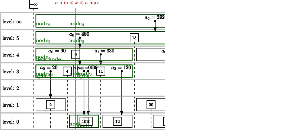
(a) Before the deletion of $k=9$. Nodes selected for $N$ are shown with green thick contours. Partition of $N$ is as follows: $\bar{n}=\mbox{node}_{4}$, $U=\{\mbox{node}_{4},\mbox{node}_{5},\mbox{node}_{6}\}$, $L=\{\mbox{node}_{2}\}$, $R=\{\mbox{node}_{1},\mbox{node}_{3}\}$.

(b) State of $T$ after the execution of the algorithm. The node shown with green thick contour derives from the merge of $\mbox{node}_{2}$ and $\mbox{node}_{3}$, $\mbox{node}_{4}$ was removed, the execution set $\mbox{node}_{1}.\mbox{min}=4$ (was $\mbox{node}_{1}.\mbox{min}=9$ before).

Figure 7: Example of execution of Algorithm 6: deletion of key $k=9$. The aggregation function is SUM and for each $k$ its value is $v=10k$.

Deletion. Algorithm 6 shows the procedure to delete a key $k$ in $T$ under the hypothesis that $k$ is already present in $T$. See Figure 7 for an example of execution of this algorithm. The first line performs a query to retrieve all nodes $n$ having $k$ in their range or $n.\mbox{min}=k$ or $n.\mbox{max}=k$. The nodes whose min and max are equal to $k$ are important for this algorithm, since the deletion of $k$ affects their range. This set, denoted $N$, contains a node $\bar{n}$ that contains $k$. We denote by $l$ its level. The other elements of $N$ are partitioned into three paths, $U$, $L$, $R$ corresponding to the three disjoint conditions of the query. Path $U$ is from $\bar{n}$ to the root of $T$ (like in Algorithms 4 and 5). Path $L$ ($R$) contains nodes $n$ such that $n.\mbox{max}=k$ ($n.\mbox{min}=k$). Paths $L$ and $R$ are made of descendants of $\bar{n}$ by Invariant 3. By applying Lemma 1 on the three paths, we get that the expected size of $N$ is $O(\log|T|)$. In the algorithm, $L$ and $R$ are represented as arrays having one element for each level below $l$. The $\bar{n}.\mathrm{aseq}$ is updated removing the key-value pair for $k$. The algorithm proceeds by performing opposite operations with respect to Algorithm 5, that is, nodes in $L$ and $R$ that are at the same level are merged so that they cover a range that is the union of the ranges of the merged nodes. This is done so that Invariants 2 and 3 are preserved. The resulting nodes end up to be a path of descendants of $\bar{n}$, denoted by $D$. Aggregate values that “overlap” the deleted key $k$ are not set during the merge. However, this is fixed when Invariant 4 is enforced by calling Algorithm 3 on $D||\{\bar{n}\}||U$.

Bulk/Batch insertion. The insertion of a large number of elements that are known in advance is more efficiently performed as a single operation. In particular, if the insertion starts from an empty DB-tree, the whole DB-tree can be built from scratch in main memory (supposing that this is large enough). This can be easily performed applying, for each element, a procedure similar to that shown in Algorithm 5, where sets $N$, $U$, and $D$ are got from main memory. The DB-tree in main memory is updated and kept ready for the next element of the bulk insertion. A the end, the resulting DB-tree can be written into the database in a single round, possibly using bulk insertion support provided by the DBMS.

In Section 6, we show that single insertions into DB-trees are quite slow with respect to insertion into regular tables. We can adopt a bulk-like approach to speed-up many insertions (a batch) in a non-empty DB-tree. In this case, we have to be careful to read first into main memory all the nodes that are affected by all insertions. This can be done by executing Lines 2, 5, and 7 of Algorithm 5, for each element. Note that, this can be done in one query round. We also have to keep track of deleted and changed nodes to correctly apply these changes at the end of the bulk insertion. We do not further detail these procedures that are simple variations of the algorithms shown in this section.

5.3 Comparison of DB-trees with Skip Lists and B-trees

Now, we present a detailed comparison of DB-trees with skip lists [47] and B-trees [15].

The most important distinguishing feature of DB-trees is related to the representation of relationships between nodes. In DB-trees, we do not store any pointer in the nodes: a parent-child relationship between nodes $n_{1}$ and $n_{2}$ is implicitly represented by a containment relationship of $\mathrm{range}(n_{1})$ and $\mathrm{range}(n_{2})$, where the extremes of ranges are explicitly represented in the nodes. This approach allows us to obtain a path to the root in a single query round and makes DB-trees very well suited to be represented in databases. On the contrary, skip lists and B-trees do use explicit pointers, thus implicitly assuming that pointer traversal is an efficient primitive operation, which is not true for databases.

Another fundamental difference with respect to common data structures is that DB-trees are targeted to support aggregate range queries and authenticated data structures, and are not targeted to speed up search. In fact, DBMSes already perform searches very efficiently. On the contrary, DB-trees rely on DBMS search efficiency to speed up aggregate range queries. DB-trees reach this objective without relying on traversals.

In Section 4.1, we described DB-trees starting from skip lists. In fact, each skip list instance is in one-to-one correspondence with a DB-tree instance. Both data structures associate levels with keys and the level of each key is selected in the same random way. However, while a skip list redundantly stores a tower of elements for each key, the corresponding DB-tree stores each key only once: essentially only the top element of the tower is represented. Further, in a DB-tree, sequential keys in a level may be grouped into a single node equipped with some metadata (level, min, and max) that allow them to be efficiently retrieved from the database. In DB-trees, a node is the smallest unit of data that is selected, retrieved, or updated when the DBMS is contacted. Due to all these differences, algorithms performing operations on DB-trees turns out to be very different from the corresponding algorithms for skip lists. Since the level associated with each key is the same in DB-trees and skip lists, statistical properties of DB-trees (see Section 4.4) also hold for skip lists (e.g., Lemma 1), or can be recast to be applicable in the skip list context (e.g., in the skip list context, Property 4 can be interpreted as related to the expected number of consecutive tower-top elements in a level).

While statistical aspects of DB-trees are very similar to skip list ones, storage aspects are somewhat similar to B-trees. In B-trees, each node $n$ is meant to be stored in a disk block and contains a selection of keys (or key-value pairs) interleaved by pointers to blocks storing the children of $n$. In both DB-trees and B-trees, descendants of $n$ store keys that are between two keys that are consecutively stored in $n$. In B-trees, each node can contain a number of keys between $d$ and $2d$, where $d$ is a fixed parameter. Hence, a node can have a number of children between $d+1$ and $2d+1$. In DB-trees, each node contains at least one key, but there is no maximum number of keys for a node. The number of keys in a node is only statistically constrained (see Property 4). Insertion of a new key in a B-tree occurs in a node that is deterministically identified and may provoke the split of zero or more nodes, possibly all the way up to the root of the tree, in order to respect the maximum number of keys per node. In DB-trees, the node $n$ where a new key is inserted is at a level that is randomly selected, possibly creating a new one if needed. Insertion of a key into node $n$ may provoke the split of nodes below $n$ to respect Invariant 3. Deletion in B-trees may require re-balancing through rotations to respect the minimum number of keys per node. In DB-trees deletion of a key from node $n$ may provoke the merge of nodes below $n$, which is exactly the opposite of what occurs during insertion. The maximum depth of a B-tree is $\left\lfloor\log_{d}(x+1)/2\right\rfloor$, where $x$ is the number of keys in the B-tree [16]. The depth of the DB-tree is only statistically characterized (see Lemma 1).

Finally, we note that the depth of a B-tree and the number of levels of a skip list are closely related to the efficiency of the operations on the respective data structure. For DB-trees, the depth of the tree is related to the size of the data that should be handled by any operation. As described in Section 5, DB-tree operations, which are locally performed by the overlay logic, take a time that is proportional to the handled data and hence turns out to be $O(\log|T|)$ on average, as for skip lists. However, it should be noted that the selection of nodes involved in a query or change is not performed by the implementation but is delegated to the DBMS. Its ability in efficiently executing the queries requested by the overlay logic has a significant impact on the overall performance (see also the experiments reported in Section 6).

6 Experiments

We developed a software prototype with the intent to provide experimental evidences of the performances of our approach.

The objectives of our experiments are the following.

1. We intend to show the response times of aggregate range queries that we obtain by using DB-trees. We expect them to be ideally logarithmic in the size of the selected range. We compare them against the response time obtained by using a plain DBMS with the best available indexing.

2. We intend to measure the response time for insert and delete operations using DB-trees and compare them against the response time of the same operations performed using a plain DBMS.

Tests were performed on a high-performance notebook with 16GB of main memory (SDRAM DDR3), M.2 solid-state drive (SSD), Intel Core i7-8550U processor (1.80GHz, up to 4.0GHz, 8MB Cache). To understand the behavior of our approach on a less performant hard-disk-based system, we also performed the tests on an old machine equipped with Intel Core 2 Quad Q6600 2.4GHz, 8 GB of main memory and a regular hard disk drive (HDD). In the following, the two platforms are shortly referred to as SSD and HDD, respectively. Both platforms are linux-based and during the tests no other cpu-intensive or i/o-intensive tasks were active.

We repeated all experiments with two widely used DBMSes: PostgreSQL (Version 11.3) and MySql (Version 8.0.16). DBMSes were run within docker containers, however, no limitation of any kind was configured on those containers.

Our software runs on the Java Virtual Machine (1.8). Since the JVM incrementally compiles the code according to the “HotSpot” approach [43], for each test we took care to let the system run long enough before performing the measurements, to be sure that compilation activity was over: we run the whole tests more than once and consider only the times measured in the last run. The DB-tree code is written using the Kotlin programming language and adopt the standard JDBC drivers for the connection with the DBMSes. Time measurements are performed using the Kotlin standard API measureNanoTime, that executes a given block of code and returns elapsed time in nanoseconds. In our experiments, we set the GO-UP probability for DB-trees to 0.5 (see Section 4.1).

Regarding Objective O1, we prepared a dataset of 1 million key-value pairs, whose keys are the integers from 1 to 1 million and whose values are random integers. We randomly shuffled the pairs and inserted them into the DBMS. For testing the plain DBMS, we created a table with two columns, with the key of the pair as primary key of the table, and the two possible indexes on (key, value) and on (value, key). For the table that represents the DB-tree, we have columns for $n.$min, $n.$max, $n.$level, plus a column that contains a serialized form of the whole node. We do not perform any selection on this last column. Its content is just returned to the client. We configured ($n.\mathrm{min}$, $n.\mathrm{max}$, $n.\mathrm{level}$) as the primary key index and ($n.\mathrm{max}$, $n.\mathrm{min}$, $n.\mathrm{level}$) as index. In both PostgreSQL and MySQL, indexes are plain B-trees. In MySQL, primary key indexing is clustered.

Insertion of DB-trees was performed with a prototypical implementation of the bulk insertion approach described in Section 5.2. The time taken for bulk insertions are reported in Table 1.

We show tests using the SUM aggregation function, which is a very widely used one and whose optimization is likely to be an objective of DBMS designers. In the tests based on a plain DBMS, we performed SQL queries like the following, where we used self explanatory names.

SELECT SUM(value)
FROM test_table
WHERE range_start<=key AND key<=range_end

For the DB-trees tests, we used our realization of Algorithm 2.

Actually, we also performed the same tests with aggregation functions MIN, MAX, COUNT, and AVG. The MIN and MAX functions are highly optimized in both DBMSes, and queries take very small time to execute, independently from the size of the range. Hence, there is no point in using DB-trees for MIN and MAX, at least in the considered DBMSes. On the contrary, the results for tests with COUNT and AVG are very much like those that we show for function SUM, hence we decided not to show additional charts for them.

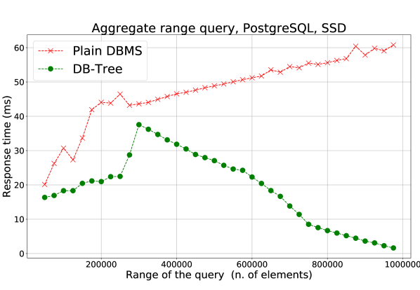
Figure 8: Performances of aggregate range queries with a PostgreSQL DBMS, on the SSD platform.

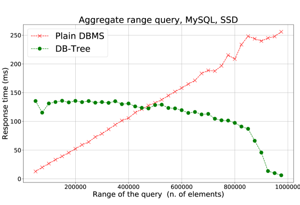
Figure 9: Performances of aggregate range queries with a MySQL DBMS, on the SSD platform.

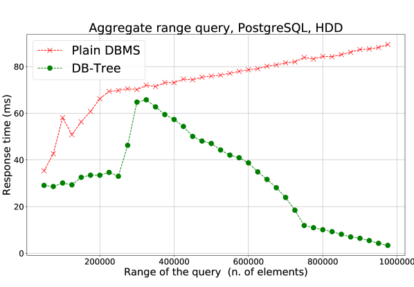
Figure 10: Performances of aggregate range queries with a PostgreSQL DBMS, on the HDD platform.

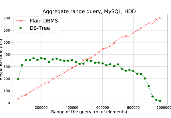
Figure 11: Performances of aggregate range queries with a MySQL DBMS, on the HDD platform.

We generated the queries to be performed for the tests in the following way. We considered range sizes from 50.000 to 975.000, with steps of 25.000. For each range size, we executed 200 queries with random ranges of that size (i.e., with a random shift) and took the average of execution times. The dataset and the ranges are the same for the tests using plain DBMSes and for the tests using DB-trees.

Queries are executed without any delay in between. Results are shown in Figures 8 and 9, for platform SSD, and in Figures 10 and 11, for platform HDD. In each figure, the x-axis shows the size of the range and the y-axis show the query duration in milliseconds. Figures show performances for tests on plain DBMSes and for tests adopting DB-trees. Using plain DBMS queries, the response time for the aggregate range query is linear, for both PostgreSQL and MySQL. The tests show that, using DB-trees, the response time is limited and well below the one obtained using plain DBMS queries, starting from a certain range size. Concerning the shape of the curves, we note that aggregate range queries are theoretically easy in two extreme cases (i) when the range is just a tuple, in this case an aggregate range query is equivalent to a plain selection, and (ii) when the range covers all the data, in this case a good strategy is to keep an accumulator for the whole dataset. In all charts related to aggregate range queries, we note that the curve for DB-trees response time is somewhat bell-shaped, reflecting that hard instances are in the middle between the two extreme cases just mentioned.

We point out that the DBMS internally performs several non-obvious query optimizations that can profoundly change the way the same kind of query is performed on the basis of estimated amount of data to retrieve. A clear effect of this can be seen in the roughly piecewise linear trend, shown in Figures 8 and 10, for the performances of aggregate range queries in PostgreSQL for plain DBMS tests. Further, comparing charts for SSD and HDD platforms, we notice the expected degradation due to the slower HDD technology and a less regular behavior for the HDD case. However, trends are quite similar for both platforms for all cases.

Concerning space occupancy on disk, this clearly depends on actual data types, indexes, and DBMS used. As an example, for the above described experiments, the occupancy is summarized in Table 1. We report occupancy of data and indexes for a plain table, i.e., the one used for plain DBMS tests, and for the table used for DB-tree tests. We note that, the number of rows in the DB-tree table is about half of the number of rows of the plain table. In fact, in our representation each row represents a node and each node contains one or more key-value pair. For PostgreSQL, the size of the data for the DB-tree is roughly the same as the size of the data for the plain table, while indexes are larger for the latter. For MySQL, the size of the data for the DB-tree is about twice the size of the data for the plain table, while indexes are comparable.

DBMS		Rows	Tot. Sz.	Data Sz.	Index Sz.	Bulk Ins. Time
PostgresSQL	Plain	1M	124MB	42MB	82MB	35s
	DB-Tree	505K	89MB	43MB	46MB	19s
MySQL	Plain	1M	81MB	43MB	38MB	2m35s
	DB-tree	505K	118MB	86MB	32MB	50s

Table 1: Disk space occupancy and bulk insertion times for data used in the experiments of Section 6.

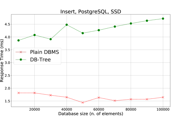
Figure 12: Performance of the insert operation of a key with a PostgreSQL DBMS, on the SSD platform.

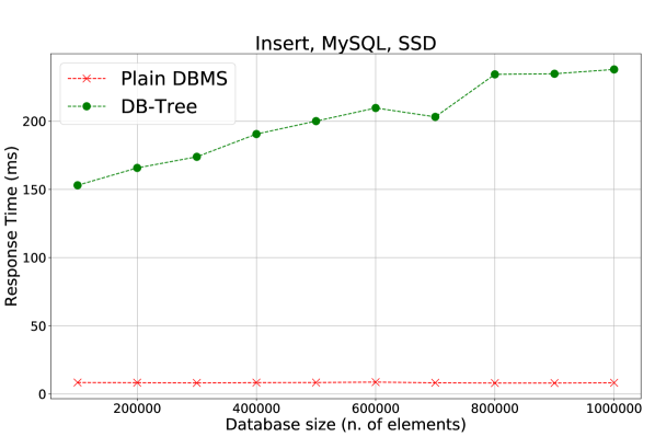
Figure 13: Performance of the insert operation of a key with a MySQL DBMS, on the SSD platform.

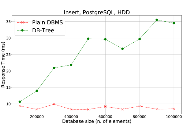
Figure 14: Performance of the insert operation of a key with a PostgreSQL DBMS, on the HDD platform.

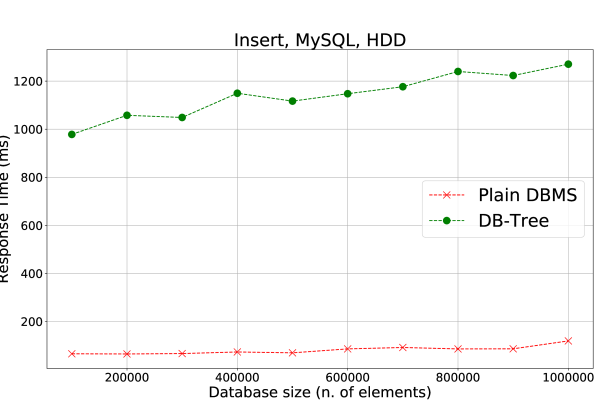
Figure 15: Performance of the insert operation of a key with a MySQL, on the HDD platform.

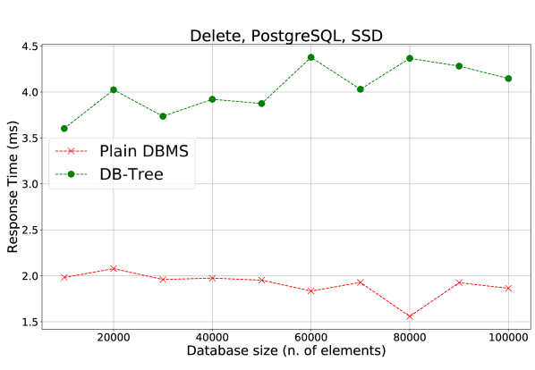
Figure 16: Performance of the delete operation of a key with a PostgreSQL DBMS, on the SSD platform.

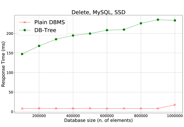
Figure 17: Performance of the delete operation of a key with a MySQL DBMS, on the SSD platform.

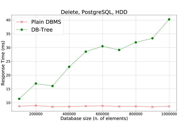
Figure 18: Performance of the delete operation of a key with a PostgreSQL, on the HDD platform.

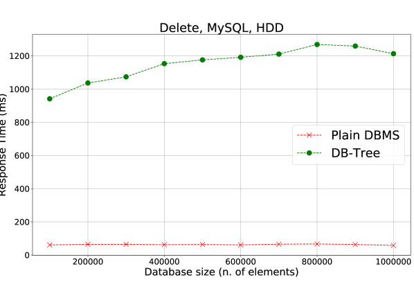
Figure 19: Performance of the delete operation of a key with a MySQL, on the HDD platform.

Concerning Objective O2, we created 10 datasets containing from 100.000 to 1 million key-value pairs, with step of 100.000. For each dataset, we created the corresponding databases for both plain DBMS tests and for DB-trees tests. Tables and indexes are as for Objective O1. To test insert response time, we preformed 200 insertions of random keys that were not in the dataset. For each of them, we measured the response time and then deleted the just inserted key to keep the dataset size constant. Operations are executed without any delay in between. Results are shown in Figures 12 and 13, for platform SSD, and in Figures 14 and 15, for platform HDD. In these figures, the x-axis shows the size of the number of key-value pairs in the database and the y-axis shows the response time in milliseconds.

Analogously, we measured response time for deletion. We preformed 200 deletions of random keys that were present in the dataset. For each of them, we measured the response time and then re-inserted the just deleted key-value pair to keep the dataset size constant. Results are shown in Figures 16 and 17, for platform SSD, and in Figures 18 and 19, for platform HDD. Axes are as in the figures for insert tests. Operations are executed without any delay in between for all cases, but for the experiment shown in Figure 19. In fact, in this case, with no delay, we observed an anomalous ramp-up trend, which we think was due to the exceeding of the maximum throughput of the system. In this case, we performed the test waiting 400ms after each operation.

As expected, charts show that, adopting DB-trees, insert and delete operations are more costly. For plain DBMS tests, the response time looks essentially constant. This is likely due to the fact that changes are just written in a log before acknowledging the operation to the client, and operations are all equal in size. On the contrary, for DB-trees, we can see a slow but clearly increasing trend, which conforms to the expected logarithmic trend predicted by the theory. In fact, also in this case operations are just stored in a log, but the number of actual operations requested to the DBMS is logarithmic. For our experiments, when using DB-trees, the slow-down factor for both insert and delete operations is within 2-4, for PostgreSQL, and within 10-20, for MySQL. These factors are quite independent from the kind of platform adopted (i.e., SSD vs. HDD).

About the comparison of charts for SSD and HDD platforms, the same remarks we made for Objective O1 applies.

7 Supporting Group-By Range Queries

In this section, we address a common need that is slightly more complex than an aggregate range query. We deal with the aggregation of values of a certain column performed on the basis of distinct values of a second column limited to a certain range of a third one. This need is usually fulfilled using the SQL construct GROUP-BY and we refer to this kind of queries as group-by range queries.

ΨSELECT Department, SUM(Amount)
ΨFROM Sale
ΨWHERE ’2010-02-01’ <= Date
Ψ       AND Date <= ’2010-03-15’
ΨGROUP BY Department
Ψ

Figure 20: Example of GROUP-BY range query.

For example, suppose to have a table that represents the sales of goods performed by each department of a company for each day, and we want to know the total sales in a specific period for each department. Suppose the table is called Sale and has columns Department, Date, and Amount. Figure 20 shows an example of group-by range query to obtain this result, for an arbitrary range, expressed in plain SQL.

To exploit DB-trees with this purpose, we define the key of the DB-tree to be the pair (Department, Date), where Department is the most significant part. A possible approach to perform the query, is to execute a plain query to obtain the distinct departments $d_{1},d_{2},\dots$ and then execute, in parallel, Algorithm 2 for each department with ranges ($d_{1}$, start_range)-($d_{1}$, end_range), ($d_{2}$, start_range)-($d_{2}$, end_range), etc. With this approach, we perform two query rounds. In the second round, we perform a number of independent queries (one for each department) and each of them is independently optimized by the query planner.

Algorithm 7 This algorithm performs a group-by range query on a DB-tree and its associated regular data table.

1:A regular data table $D$ with columns $x$, $y$ and $v$, an associated DB-tree $T$ on all keys $(x,y)$ with associated values $v$, and two values $y^{\prime}$ and $y^{\prime\prime}$ (with $y^{\prime}<y^{\prime\prime}$).

2:A set of pairs in the form $(x,\alpha_{x})$, such that $\alpha_{x}=\alpha(v_{1},\dots,v_{r_{x}})$, where $r_{x}$ is the number of rows of $D$, selected such that they have the given $x$ and have $y^{\prime}\leq y\leq y^{\prime\prime}$, and $v_{1},\dots,v_{r_{x}}$ are the values for $v$ for those rows of $D$ (and corresponding key-value pairs in $T$).

3:$\triangleright$ Execute Lines 4-7 in one query round.

4:$\bar{L}\leftarrow$ nodes $n$ from $T$ such that $y^{\prime}<n.\mathrm{max}.y\leq y^{\prime\prime}$ AND $(n.\mathrm{min}.y<y^{\prime}$ OR $n.\mathrm{min}.x\neq n.\mathrm{max}.x)$.

5:$\bar{R}\leftarrow$ nodes $n$ from $T$ such that $y^{\prime}\leq n.\mathrm{min}.y<y^{\prime\prime}$ AND $(y^{\prime\prime}<n.\mathrm{max}.y$ OR $n.\mathrm{min}.x\neq n.\mathrm{max}.x)$.

6:Let $X$ denotes the distinct values of $x$ in $D$.

7:$\bar{N}\leftarrow$ pairs $(x,n)$ such that $x\in X$, $n$ is in $T$, $n.\mathrm{min}<(x,y^{\prime})<(x,y^{\prime\prime})<n_{x}.\mathrm{max}$, and $n.\mbox{level}$ is minimum.

8:For all $x\in X$

9:  let $n_{x}$ be the node associated with $x$ in $\bar{N}$,

10:  let $L_{x}$ be sequence of nodes $n$ in $L$ with $n.\mathrm{max}.x=x$,

11:  let $R_{x}$ be sequence of nodes $n$ in $R$ with $n.\mathrm{min}.x=x$.

12:Let $S$ be an empty set.

13:for all triples $\langle n_{x},L_{x},R_{x}\rangle$  do

14:     Execute Algorithm 2 starting from Line 7 with $\bar{n}\leftarrow n_{x}$, $L\leftarrow L_{x}$, $R\leftarrow R_{x}$ and with $k^{\prime}\leftarrow(x,y^{\prime})$ and $k^{\prime\prime}\leftarrow(x,y^{\prime\prime})$. In executing Algorithm 2, modify the behavior of Lines 9, 14, and 18 so that aggregate values next to a key that have the most significant part $\neq x$ should be ignored (since they are not related to group for $x$).

15:     Let $\alpha_{x}$ be the result of the above call to Algorithm 2.

16:     Add $(x,\alpha_{x})$ to $S$.

17:end for

18:return $S$

We now show that, adopting DB-trees, we can perform the above query in one query round using only three distinct queries as in Algorithm 2. The procedure is shown in Algorithm 7, which is a variation of Algorithm 2. We assume a setting with a regular data table $D$, containing the data, and additional overlay-table $T$ containing a DB-tree, also denoted by $T$ and coherent with $D$ (see Section 3.3). We assume that $D$ has columns $x,y,v$ and that the user intends to perform aggregation on column $v$, grouping on column $x$, while selecting a range on column $y$. For simplicity, in the following, we use symbols $x$, $y$ and $v$ to denote both column names and the corresponding generic values of the columns. To build the DB-tree $T$, we consider all the triples $(x,y,v)$ taken from the rows of $D$ considering each pair $(x,y)$ as key and $v$ as its corresponding value. We intend $x$ to be the most significant part of the key, regarding ordering in $T$.

The first objective of Algorithm 7 is to obtain from $T$, node $n_{x}$, and sequences $L_{x}$ and $R_{x}$, for each distinct $x$ in $D$. These play the same role that $\bar{n}$, $L$ and $R$ play in Algorithm 2. Then, the part of Algorithm 2 that can run in main memory is performed on each triple $\langle n_{x},L_{x},R_{x}\rangle$ to obtain each row of the result. Lines 4-7 retrieve all the data needed in one round. Then, we proceed with computations performed in main memory. Nodes in $\bar{N}$, $\bar{L}$, and $\bar{R}$ are sorted out into their respective $n_{x}$, $L_{x}$ and $R_{x}$, in Lines 9-11. Finally, we execute a procedure very similar to that of Algorithm 2, for each group, i.e., for each value of $x$. The only notable change is to additionally check that aggregations take into account only aggregate values between keys having $x$ as most significant part. In fact, if this is not true, the aggregate value is not related to the current group (or at least not completely) and should be ruled out.

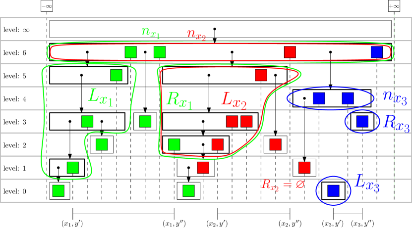
Figure 21: An example of DB-tree evidencing sets $L_{x}$, $R_{x}$, and $n_{x}$ for a group-by range query executed by Algorithm 7. The details are explained in the text.

⬇

SELECT DISTINCT ON (S.x) x, $T$.*

FROM $T$, (SELECT DISTINCT x FROM $D$) AS S

WHERE ((min_x = S.x and min_y < $y^{\prime}$) OR min_x < S.x) AND

((max_x = S.x and max_y > $y^{\prime\prime}$) OR max_x > S.x)

ORDER BY S.x, level

Figure 22: Example of SQL query (in PostgreSQL dialect) to obtain $\bar{N}$ in Algorithm 7.

Figure 21 shows an example of DB-Tree on which a group-by range query is performed. Squares of distinct colors correspond to keys with distinct values of $x$ (green for $x_{1}$, red for $x_{2}$, and blue for $x_{3}$). The range on $y$ is given by $y^{\prime}$ and $y^{\prime\prime}$. Lines on the bottom of the figure represent ranges for each value of $x$. Colored contours show, for each value of $x$, the nodes in $n_{x}$, $L_{x}$, and $R_{x}$. Note that, nodes related to distinct groups (i.e., for distinct values of $x$) may overlap.

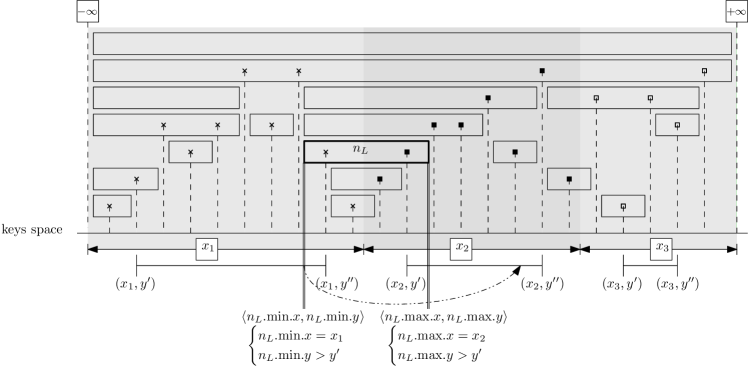
Figure 23: A case handled by Algorithm 7 in a special way. Node $n_{L}$ spans more than one value for $x$. See text for details.

It is useful to make some remarks on Lines 4-7. Line 4 introduces a further condition with respect to what we find in Algorithm 2. In fact, by requiring only $n.\mbox{min}.y<y^{\prime}<n.\mbox{max}.y\leq y^{\prime\prime}$, as in Algorithm 2, we would have collected many nodes whose ranges intersect $(x,y^{\prime})$ for any $x$, but not all of them. In particular, if a node has its range that spans more than one value of $x$, it may occur that $n.\mbox{min}.y<y^{\prime}$ is not true, but the node intersect a certain $(x,y^{\prime})$. The condition $n.\mathrm{min}.x\neq n.\mathrm{max}.x$ includes all the missing cases. Symmetrically, the same holds for Line 5. Figure 23 shows an example of this case. In this figure, node $n_{L}$ is required to compute aggregate for the group between $(x_{2},y^{\prime})$ and $(x_{2},y^{\prime\prime})$. However, since $n_{L}.\mbox{min}.y>y^{\prime}$, $n_{L}$ turns out not to be selected when only the condition $n.\mbox{min}.y<y^{\prime}<n.\mbox{max}.y$, of Algorithm 2, is considered. On the contrary, $n_{L}$ is selected by the condition $n_{L}.\mbox{min}.x\neq n_{L}.\mbox{max}.x$ considered in Algorithm 7, since $n_{L}.\mbox{min}.x=x_{1}\neq x_{2}=n_{L}.\mbox{max}.x$.

About Line 7, performing this operation with one SQL query is not obvious. In Figure 22, we show an example of this query using the PostgreSQL dialect. The DISTINCT ON (S.x) clause returns only rows with distinct values for S.x. The chosen one is the first according to the ORDER BY semantic. We use the regular data table $D$ to obtain all values for $x$. Other approaches are possible to get all values of $x$ when only $T$ is present. We do not go into the details of the schemes that can be used for $T$. We just note that, for what described before this section, there is no reason to represent keys contained in nodes in a way that can be easily extracted by a query. This is also not trivial to do in a relational database, since their number for each node can vary (see Section 6). This is the main reason why we described our solution assuming to have a regular DBMS table $D$ as an input to Algorithm 7.

The correctness of this algorithm derives form the fact that, by construction, ranges for each $x$ do not overlap (see Figure 21) and by the correctness of Algorithm 2. Further, we note that, elements of aggregate sequences of retrieved nodes that aggregate values for keys with different value of $x$ are never used by Algorithm 7.

7.1 Experiments with DB-Trees for Group-By Range Queries

We performed some experiments to assess the performance of Algortihm 7 on realistic data. In Section 6, we noted that DB-trees are more advantageous for aggregate range queries with large ranges. As we show in the following, this is also true for group-by range queries. The dataset we used for our experiments is derived from the TPC-H benchmark [17]. From that dataset, we considered the lineitem table containing about six millions of rows. We picked columns L_suppkey (numeric IDs), L_shipdate (dates that span seven years), and L_extendedprice (floating point numbers). We focused on a query that aggregates the values of L_extendedprice grouping by distinct values of L_suppkey on ranges defined on L_shipdate. Other columns were not imported into our test database. To support this group-by range query, we had to choose, as key of the DB-tree, the pair (L_suppkey, L_shipdate). For this pair, TPC-H contains duplicated values, which is not compatible with our prototypical implementation of DB-trees. To circumvent this problem, we transformed each date to a timestamp adding a random time. To show performances of DB-trees in a range where they can provide a substantial benefit, we modified values in L_suppkey as follows. The original dataset contains 10,000 distinct values in L_suppkey. We replaced each value $x$ in L_suppkey with $x\mod 20$ to obtain 20 distinct values. In this way, we obtained 20 groups, each one containing a number of elements that is large enough to show the effectiveness of the adoption of DB-trees. We refer to the resulting dataset as modified TPC-H. Since elements are quite uniformly distributed over the groups, each group turns out to contain about 300,000 elements, for the whole dataset. The application of range selection reduces it. This reduction is quite regular, since values in L_shipdate are uniformly distributed over groups and over time. We performed our experiments with PostgreSQL (SSD platform). During the preparation of the experiments, we realized that PostgreSQL is not able to perform a thorough optimization of the query shown in Figure 22. We substituted it with that shown in Figure 24. We also added a column f to the overlay table $T$ to contain character ’t’ if the result of min_x <> max_x for the node is true, ’f’ otherwise.

⬇

(SELECT * FROM $T$

WHERE ((min_y < $y^{\prime}$) AND (max_y > $y^{\prime\prime}$ )))

UNION

(Select * FROM $T$ WHERE f = ’t’)

Figure 24: Optimized version of the query shown in Figure 22 that was adopted for testing group-by range queries. See text for further details.

Actually, this query returns a larger set of nodes with respect to the query shown in Figure 22. In fact, the new query always returns all nodes whose range overlaps group boundary (i.e., all nodes with f = ’t’). To obtain $\bar{N}$ (see Algorithm 7), a further selection is performed in memory by the overlay logic software when data are received. On table $T$, we configured plain B-tree indexes on f and on (min_y, max_y). We also measured execution times for the plain DBMS query on the regular table, where we configured a primary key on (L_suppkey, L_shipdate). In PostgreSQL, this means that a B-tree index kept on that columns. Since dates in L_shipdate are uniformly distributed over time, it was easy to pick random ranges such that each group contained a number of elements from 50,000 to 300,000, with steps of 50,000. For each step, we queried 200 different random ranges (i.e., each with a random shift of the range) and we took the average of the execution times. The results, shown in Figure 25, confirms that DB-trees outperform the plain DBMS query on the regular table for ranges that give rise to groups with large number of elements: greater that 200,000 in our case.

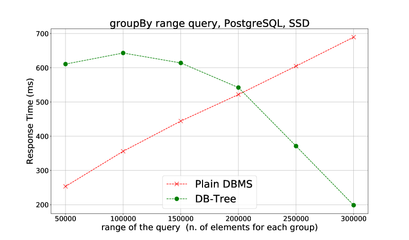
Figure 25: Performances of the execution of group-by range queries on PostgreSQL (SSD platform), on the modified TPC-H dataset.

7.2 Comparison with Materialized Views

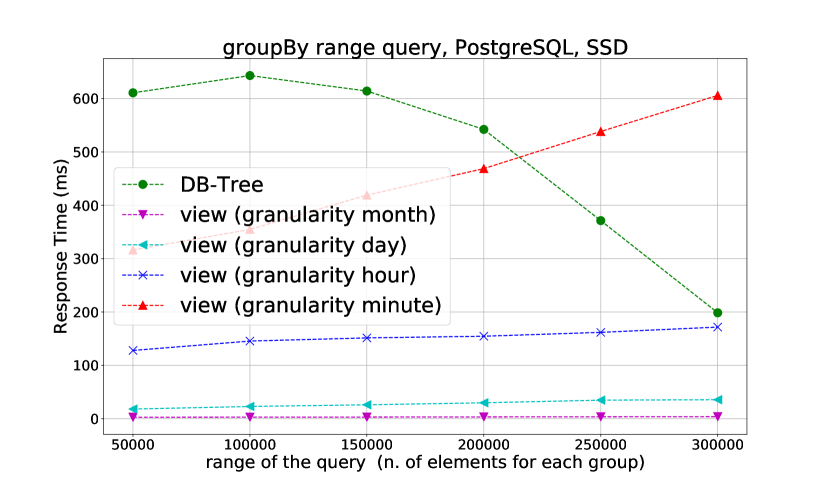
Figure 26: Performances of group-by range queries. Materialized views vs. DB-Trees on PostgreSQL (SSD platform), on the modified TPC-H dataset.

Granularity	Refresh time	N. Rows
Month	5s	1672
Day	6s	50,488
Hour	8s	1,145,760
Minute	12s	5,683,522

Table 2: Refresh times and size of materialized views used in our experiments.

We run the same tests for group-by range queries using materialized views, to understand how this common technique compare with DB-trees. We performed our experiments using PostgreSQL. For the same dataset adopted in the above experiments, we created materialized views at different granularities: month, day, hour, and minute. We executed the same group-by range queries described above on these materialized views and we measured execution times. We picked ranges giving a number of elements per group between 50,000 and 300,000, with steps of 50,000 and 200 random queries, as above, for each step. Figure 26 shows the execution times taken by the queries performed on the materialized views vs. execution times of the same queries performed using DB-trees. For materialized views, the execution time increases linearly with the number of elements contained in each group, while it decreases for DB-Trees. However, DB-Trees perform better only for minute granularity, in our tests. Since the query is performed on aggregated data, the precision of the result of the queries performed on materialized views depends on the granularity of the view. It is possible to obtain precise results by independently querying the extremes of the range but we did not performed any experiment regarding this aspect. In fact, we think that the above results already show the great potentiality of materialized views. Table 2 shows the time taken to refresh the whole materialized view. They are between 5 and 12 seconds for our dataset. The number of rows of the views are also reported. We note that materializing with minute granularity provides very little benefit, since the original table contains 6,001,215 rows.

From the trend shown by our experiments, DB-trees may result to be a better approach than materialized views when the number of elements in the groups are very large and this is not compensated by the coarseness of the granularity. This may occur in practice, since granularities of materialized views are statically decided in advance, while queries might be on ranges whose size can vary across several orders of magnitude. For example, this may occur in graphical systems if the user is allowed to zoom in and out on a timeline and a corresponding histogram for the current zoom level should be shown. DB-trees have a substantial overhead but they are adaptive, in the sense that no decision in advance is needed about the order of magnitude of the ranges to be queried. Further, we recall, that DB-trees may be the only viable solution in situations in which the DBMS does not natively support the needed aggregation function.

7.3 Comparison with VerdictDB

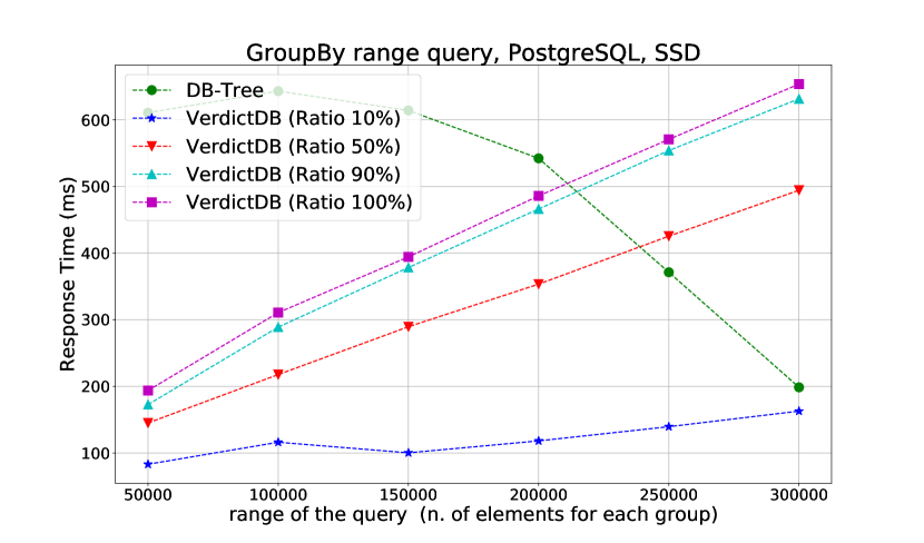
Figure 27: Performances of VerdictDB vs. group-by range queries using DB-Trees on PostgreSQL (SSD platform), on the modified TPC-H dataset.

We now compare our DB-tree approach for the execution of group-by range queries with the solution provided by VerdictDB [45]. VerdictDB is a very interesting tool that practically realizes an approximate query processing technique. It allows the user to perform group-by range queries choosing a trade-off between speed and precision of the result. It relies on regular relational DBMS to store data. The user can ask the creation of a “sampled” version of a table, called scramble, with a certain size ratio. Higher size ratios provide better precision at the expense of longer execution time. We performed our experiments using PostgreSQL (SSD platform) as underlying DBMS. For the same dataset adopted in the above experiments (modified TPC-H), we created several scrambles with different size ratios: 10%, 50%, 90%, and 100%. We executed the same group-by range queries described above on all scrambles. We again picked ranges giving a number of elements per group between 50,000 and 300,000, with steps of 50,000, running 200 different random queries in each step, as in Sections 7.1 and 7.2.

VerdictDB is very efficient when the size ratio is low. In any case, execution times increase linearly with the number of elements contained in each group, as for the execution using the plain DBMS approach. In Figure 27, we show the time taken by VerdictDB to process the group-by range query for increasing range sizes using the four size ratios mentioned above. For a clear comparison, we also report the time taken by our approach based on DB-trees. The comparison is favorable to our approach when the number of elements in the groups is large and when the size ratio is not too low. Since a low size ratio negatively impacts the precision of the results produced by VerdictDB, we also measured errors. In Table 7.3, we reported, for each point of the chart in Figure 27 that is related to VerdictDB results, the maximum error we obtained, relative to the correct answer. Each shown percentage is the maximum of the relative errors across all the queries (200) that we run for each step. These results are specific for our case and are only useful for the purpose of comparison with the DB-tree approach in this specific test. A broad description of VerdictDB with respect to precision can be found in [45].

In our experiments, the time taken by VerdictDB to generate the scramble from scratch is always about 6 seconds.

Scramble Size Ratio	Number of Elements for Each Group
	50K	100K	150K	200K	250K	300K
10%	5.18%	3.79%	2.87%	1.99%	1.54%	1.45%
50%	2.44%	2.53%	2.0%	1.74%	1.56%	1.53%
90%	3.0%	2.0%7	1.89%	1.35%	1.35%	1.26%
100%	3.02%	2.02%	1.76%	1.43%	1.18%	1.2%

Table 3: Maximum relative errors of results of group-by range queries using VerdictDB. See text for details.

The most evident difference between DB-trees approach and VerdictDB is that DB-trees always produce an exact result, while results produced by VerdictDB may have non-negligible errors. It depends on the application how much precision can be traded for speed. In any case, when the number of elements in the groups are large, the DB-tree approach outperform VerdictDB even for moderately small size ratios. For example, in our case, when the number of elements for each group is 250,000 or more, DB-trees provide exact results and perform better even if VerdictDB is used with a size ratio of 50%, which gives a maximum error of about 1.5% in our case.

8 Supporting Authenticated Data Structures

In this section, we show how it is possible to use DB-trees to support Authenticated Data Structures (ADS). We briefly introduce ADSes with their properties and show a typical use case. Then, we show how we can use DB-trees as a persistent and efficient ADS.

An Authenticated Data Structure (ADS) is an ordered container of elements that deterministically provides a constant-size digest of its content that has the same properties of a cryptographic hash. We call this digest the root-hash of the ADS, and we denote it by $r$. For our purposes, we limit ADSes to contain implicitly ordered elements, like key-value pairs. In other words, we regard ADSes as search trees augmented with security features. If the content of the ADS changes, $r$ changes. Further, it is hard to find two sets of elements with the same root-hash. An ADS provides two operations: authenticated query and authenticated update. A query returns the queried element and the proof, associated with a certain $r$, that the result is indeed among the elements of the ADS instance having that $r$ as root-hash. If a trusted entity safely stores the current $r$, it can query the ADS and execute a cryptographic check of the proof against its trusted version of $r$ to verify that the query result matches what expected. The update operation on key $k$ changes $v$ associated with $k$ into a provided $v^{\prime}$ and changes $r$ in $r^{\prime}$, as well. Insertion and deletion also change $r$. The interesting aspect is that a trusted entity that intends to update the ADS should be able to autonomously compute $r^{\prime}$ starting from the proof of the elements that are changing.

Figure 28: An example of Merkle Hash Tree with four leaves and a binary structure. We evidenced the elements regarding the proof of $\langle k_{1},v_{1}\rangle$ with thick contours.

A simple ADS is the Merkle Hash Tree [39] (MHT). An example of MHT is shown in Figure 28. In our example, the MHT is a binary search tree in which every leaf is associated with a key-value pair $\left<k,v\right>$. Function $\mathrm{hash}(\cdot)$ is a cryptographic hash function. Every node $n$ is labeled by a cryptographic hash $H(n)$. If $n$ is a leaf, we define $H(n)=\mathrm{hash}(\left<k,v\right>)$. If $n$ is an internal node, with $n^{\prime}$ and $n^{\prime\prime}$ its children, $H(n)=\mathrm{hash}(H(n^{\prime})|H(n^{\prime\prime}))$. If $n$ is the root, $r=H(n)$ is the root-hash of the MHT.

A typical application of MHT is to allow a client with limited amount of resources to outsource the storage of a large amount of data to an untrusted server. The client keeps only a trusted version of the root-hash while the server keeps the MHT. The server provides proofs for each query performed by the client. A proof for a leaf is obtained by considering the path from the leaf to the root and, for each node of the path, putting the hash of the sibling into the proof (see Figure 28 for an example). This allows the receiver of the proof to be able to compute the root-hash from the content of the leaf, i.e., from the result of the query. The client can compare the resulting root-hash against its trusted copy to verify authenticity of the reply. The length of the proofs is $O(\log n)$ for balanced trees (where $n$ is the number of leaves).

Suppose that the client intends to change the value associated with a certain key $k$. Client query the server for the $k$ and get the current associated $v$ with its proof. After checking the proof against its root-hash, client can compute the new root-hash for a new value $v^{\prime}$ just performing the same computation as for proof checking but pretending the new value $v^{\prime}$ is associated with $k$. The obtained root-hash should be the root-hash of the updated MHT, and be used as trusted root-hash for subsequent queries.

A DB-tree can be adapted to serve as a persisted and efficient ADS. In this case, we call it an authenticated DB-tree. From the point of view of the algorithms, we use $\mathrm{hash}(a|b)$ as aggregation function on $a$ and $b$, and we consider cryptographic hash values as a sort of aggregate values (details are provided below). Note that, $\mathrm{hash}(a|b)$ is usually non-associative, since standard hash functions (like, e.g., SHA-2) are not associative. In this case, the concept of range query is not correctly defined, and Algorithm 2 is not useful. On the contrary, the new authenticated query operation is of interest in this context, which allows the user not only to get the value of a key but also to get the corresponding proof. Further, without associativity, the structure of the tree impacts the resulting root-hash. This is not desirable, since users would like to uniquely associate a root-hash to a given content of the ADS. To eliminate this dependency, we can “de-randomize” on the basis of the content as follows. In running Algorithm 1, to choose the level associated with a key $k$, we suppose to adopt a random generator that is initialized by a seed that we set to $k$ itself. In this way, given a key $k$, a level is deterministically associated with $k$, while keeping unchanged the statistics of the levels and the properties described in Section 4.2.

In an authenticated DB-tree, the hash of a node $n$ with $n.\mbox{aseq}=a_{0},p_{1},a_{1},\dots,a_{m-1},p_{m},a_{m}$ is $\mathrm{hash}(n)=\mathrm{hash}(a_{0}|p_{1}|a_{1}|\dots|a_{m-1}|p_{m}|a_{m})$, where each $a_{i}=\mathrm{hash}(n_{i})$ and $n_{i}$ is the corresponding child. As we did in the rest of the paper, we intend that missed $a_{i}$’s are simply omitted in the formulas. If $n$ is a leaf, it has no children, hence, its hash is computed on the concatenation of the pairs it contains, unnoticed. The root of an authenticated DB-tree contains only one hash, that is its root-hash. A proof, for a given pair $p=\langle k,v\rangle$, is the sequence $N$ of nodes that have $k$ in their range, ordered by ascending level, up to the root. This set of nodes can be retrieved in one query round and has size logarithmic in the number of elements contained in the DB-tree (see Section 5).

The client checks that the response to an authenticated query operation is genuine, by the following procedure. It computes $\mathrm{hash}(n)$ for the first node $n\in N$. For each node $n\in N$ after the first, let $n^{\prime}$ be the node that precedes $n$ in $N$. Node $n$ contains in $n.$aseq one hash that is related to the node $n^{\prime}$. This is the hash between the keys that are the closest to $k$. This hash is ignored and substituted by $\mathrm{hash}(n^{\prime})$. Then, $\mathrm{hash}(n)$ is computed and used in the next iteration. When all nodes are scanned, the hash of the root is compared with the trusted root-hash the client should have. A proof of non-existence for key $k$ has the very same structure, just the first node of $N$ does not contain a key-value pair of $k$ and the keys closest to $k$ in $n.$aseq have no aggregate value between them. The same checking procedure can be applied.

In an authenticated DB-tree, the algorithms to perform update, insertion and deletion of a key-value pair are very similar to those of the corresponding operations for a regular DB-tree. We should take care of the following aspects. When the server provides a set of nodes they should always be considered proofs and checked against the trusted root-hash of the client before proceeding. This is always possible since all DB-tree-changing algorithms deal with paths up to the root of the DB-tree. After the change, hashes, including the root-hash, are updated by the execution of Algorithm 3. After executing any changing algorithm, the client should locally store the new root-hash as the trusted root-hash to be used in the following operations.

Concerning security, we assume a threat model in which the DBMS can perform any tampering on the DB-tree with the purpose to change the key-value pairs it contains. We do not consider other kinds of attacks. The security of an authenticated DB-tree is its ability to always detect any misbehavior of the DBMS, i.e., we would like to rule out any false negative. As for Merkle Hash Trees, this is a direct consequence of the inability of the untrusted DBMS to find a collision on the adopted cryptographic hash function. In the context of ADSes, correctness means that any misbehavior detected by proof checks is a real DBMS misbehavior, i.e., we would like to rule out any false positive. Correctness of DB-trees derives directly from the ability of keeping invariants after all DB-tree-changing operations. This comprises correctly computing the hashes of all nodes, which is responsibility of Algorithm 3.

Concerning performances of authenticated DB-trees in practice, we note that all their operations interact with the DBMS using exactly the same queries as for plain DB-trees. Only the local processing performed by the overlay-logic is slightly different. In all experiments of Section 6, the time spent for the overlay-logic processing is negligible with respect to the time spent to execute the queries. For authenticated DB-trees, the overlay-logic may additionally need to check proofs performing all needed cryptographic hashes. But this turns out to be negligible, too, as we show in the following. For these reasons, in practice, authenticated DB-trees perform like regular DB-trees. In particular, for insertion and deletion, experimental results are essentially the same of those shown in Section 6, hence they are not reported here. An authenticated query for a key $k$ selects only the nodes $n$ for which $n.\mbox{min}<k<n.\mbox{max}$. We measured the average execution time of this query on the same DB-tree of 1 million elements that we used in Section 6. The time it takes on PostgreSQL (using SSD) is about 20ms (average on 200 random queries). Our instance has 23 levels, hence each query returns at most 23 nodes, which should be interpreted as the proof returned by the authenticated query performed on the authenticated DB-tree. Now, we show that the time spent to check a proof is negligible with respect to the time taken to perform the query on the DBMS. The actual verification of the proof should compute all the cryptographic hashes along the proof up to the root. In our instance, each node contains 2 key-value pairs and 3 “aggregates”, that is hashes of children, on average. To verify the proof, for each node, we have to compute the hash of the pairs plus one hash of the whole node. We performed the tests using SHA256. Each hash takes about $1.5\mu s$ to be computed. Hence, the time taken by proof verification turns out to be about $103.5\mu s$. This is four order of magnitude less than the time taken to perform the query on the DBMS.

9 Discussion of the Simplifying Assumptions

In Section 3.3, we presented general architectural problems related with overlay indexes and introduced some simplifying assumptions. The objective of this section is to discuss these assumptions, also considering the specific DB-tree approach, and show whether generalizations are simple or require further scientific investigation.

Middle layer. In Section 3.3, we mentioned the possibility to develop a query rewriting middle layer to support overlay-indexes. Query rewriting is a classical topic in database research (see, for example, [45, 26, 2, 23, 28]), but practical widely used realizations are rare. Concerning the development of a middle layer targeted to DB-trees, we identify some challenges. Firstly, query rewriting means dealing with a complex SQL syntax and its many proprietary variations. We think that the scientific interest of this aspect is marginal, but the development effort is large. Further, a middle layer may address only the exact kinds of queries shown in this paper (passing all others queries to the DBMS unchanged) or trying to support the optimization of more complex aggregate (group-by) range queries, for example comprising equality selections, two dimensional range selections, joins, etc. Some of these objectives are direct extensions of what is described in this paper, while some may require further scientific investigation. For example, suppose to have an aggregate range query $Q$ supported by a DB-tree $T$. To support $Q^{\prime}$ derived from $Q$ by including an additional equality selection on a column $c$, we can simply add $c$ as the most significant part of the key of $T$. On the contrary, the extension to more-than-one-dimension range queries is not trivial and, in our opinion, may deserve further scientific investigation (see also Section 10). In any case, the middle layer should allow the user to specify which DB-trees to build, specifying the key, the value, and the aggregation function(s) to be supported. To do that, an extension of the data definition language should be provided. The design of this extension is a critical aspect from the point of view of the usability and of the power of the resulting layer. Further, having a number of DB-trees at disposal, the middle layer should be able to rewrite certain queries taking advantage ot them, but only when this is deemed useful. This can be regarded as an optimization problem per se that may be independently studied. For example, the middle layer may choose not to rewrite an aggregated range query whose range is small.

Transactions, multiple clients, fault tolerance. In this paper, for the sake of simplicity, we deliberately avoided to consider the use of overlay-indexes and DB-trees in a context where transactions are needed. Typical situations in which this occurs is when multiple clients access the same DB-tree and when faults of the DBMS may occur. In principle, nothing prevents to execute the algorithms presented in this paper within transactions (supposing to adopt a DBMS that supports them). Algorithms 4, 5, and 6 follow the scheme showed at the beginning of Section 5.2. That is, they wait for the reply of the read round, compute the changes and perform the update round. However, the best practice is to avoid the execution of schemes like this within a transaction. In fact, a communication problem with the DBMS may keep the transaction open (and involved tables locked) until a timeout expires. A possible workaround to this problem is to move the overlay-logic within the DBMS by using stored procedures (if supported) or moving overlay-logic so close to the DBMS so that network faults cannot independently occur (for example within the same machine).

The above considerations also apply to the case in which a DB-tree is associated with a regular table. In this case, Algorithms 4, 5, and 6 should be executed in a transaction together with the change of the regular table.

When changing operations are rare, and the DB-tree is not associated with a regular table, optimistic approaches may be adopted. For example, we could perform the read round of a changing operation within a transaction and perform the update round of that operation in a distinct transaction. In the second transaction, before applying changes, it should be checked, preferably directly within the DBMS, that no change was applied (e.g., by another client) in the meantime to the DB-tree. If the check fails, the transaction should be aborted and the whole changing operation should be re-run, starting from the query round. An interesting way to perform this check is to use the same DB-tree to realize an authenticated data structure (see Section 8). In this case, the root-hash can be checked to verify if any change to the DB-tree occurred from the last read. It is possible to support an aggregation function and a cryptographic hash within the same DB-tree as explained in the following.

Multiple aggregation functions. There are cases where more than one aggregation function $\langle f_{i},g_{i},h_{i}\rangle$, for $i=1,\dots,q$, (see Section 4.2) should be supported, where each $f_{i}(\cdot)$ aggregates values in $A_{i}$, and each $g_{i}(\cdot)$ generates values in $A_{i}$ from one or more columns. Here, we refer to columns as if they were stored independently in the database in a regular data table, but this is not strictly needed (see Section 3.3). If range selections are always performed on the same key for all aggregation functions, we can build a single DB-tree to support all of them. For this DB-tree, the set $A$ (see Section 4.2) is $A_{1}\times\dots\times A_{q}$, aggregation function is defined as $f(a_{1},\dots,a_{q})=(f_{1}(a_{1}),\dots,f_{q}(a_{q}))$, and functions $g(\cdot)$ and $h(\cdot)$ are consistently defined. Note that, if the queries that we have to support perform range selections on distinct columns, to support them, we have to construct one DB-tree for each of that columns (having each of them as its key). Cryptographic hash functions can also be supported along with aggregation functions, if we take care of the fact that they are not associative (see the details in Section 8). This allows us to support the optimistic approach described at the end of the previous paragraph. In this case, checking if a DB-tree has been changed since the execution of a previous query, boils down to checking that its root-hash is unchanged.

Caching, consistency, batch insertion. In Section 3.3, we mentioned the possibility to implement caching in the overlay-logic. We also mentioned that consistency problems may arise in the case of multiple clients. This occurs when the DB-tree is changed by Algorithms 4, 5, and 6. The most obvious workaround is to broadcast all changes to all clients, so that they can update (or invalidate) their cache. This approach is very demanding in terms of networking and CPU resources, especially if changes and clients are many. We may obtain most of the benefits of caching by moving the overlay-logic close to the DBMS or by using stored procedures. In fact, in this case, the overlay-logic can quickly access the DBMS, which we suppose to have its own cache. Finally, we note that the notable case of batch insertion performed by one client described in Section 5.2 is essentially a special case of caching.

10 Conclusions and Future Work

We showed how it is possible to support aggregate range queries efficiently on conventional databases that do not implement specific optimizations. To do that, we introduced the DB-tree: a new data structure that realizes a specific type of index that is represented at the database level (an overlay-index) and can be accessed by performing regular queries to the DBMS. It can be also customized in many ways to support a wide class of aggregation functions, authenticated data structures, and group-by range queries. DB-trees can be queried downloading only $O(\log r)$ data (and hence taking $O(\log r)$ time), with $r$ the size of the data on which aggregation is performed, while common DBMSes scan $O(r)$ data and thus take $O(r)$ time to answer the same queries. Experiments show that the improvement with respect to the plain DBMS can be very large even for moderately large datasets. DB-trees introduce some overhead for insertion and deletion, which was experimentally measured to be a factor from 2 to 20 in our tests.

Regarding future research directions, from the theoretical point of view, it would be interesting to investigate a bi/multi-dimensional generalization of DB-trees to support speedup of aggregate range queries in GIS systems. This generalization may be inspired to the work of Eppstein et al. [21] about skip quadtrees.

From the practical point of view, it would be desirable to have a framework that streamlines the use of DB-trees in practical contexts, like VerdictDB [45] does for approximate query processing. Further, experiments in a big-data context may be useful to better asses the spectrum of applicability of DB-trees.

References

- [1] PostgreSQL 12.0 Documentation. https://www.postgresql.org/docs/9.4/sql-createaggregate.html [on-line 2019-10-14].
- [2] Swarup Acharya, Phillip B Gibbons, Viswanath Poosala, and Sridhar Ramaswamy. The aqua approximate query answering system. In ACM Sigmod Record, volume 28, pages 574–576. ACM, 1999.
- [3] Fabrizio Angiulli and Fabio Fassetti. Indexing uncertain data in general metric spaces. IEEE transactions on knowledge and data engineering, 24(9):1640–1657, 2012.
- [4] Andrey Borodin, Sergey Mirvoda, Ilia Kulikov, and Sergey Porshnev. Optimization of memory operations in generalized search trees of postgresql. In International Conference: Beyond Databases, Architectures and Structures, pages 224–232. Springer, 2017.
- [5] David Boutcher and Abhishek Chandra. Does virtualization make disk scheduling passé? ACM SIGOPS Operating Systems Review, 44(1):20–24, 2010.
- [6] Lisa Bromberg, Vladimir Shpilrain, and Alina Vdovina. Navigating in the cayley graph of and applications to hashing. In Semigroup Forum, volume 94, pages 314–324. Springer, 2017.
- [7] Joe Celko. Joe Celko’s Trees and hierarchies in SQL for smarties. Elsevier, 2012.
- [8] Badrish Chandramouli, Jonathan Goldstein, and Abdul Quamar. Scalable progressive analytics on big data in the cloud. Proceedings of the VLDB Endowment, 6(14):1726–1737, 2013.
- [9] Surajit Chaudhuri and Vivek Narasayya. Self-tuning database systems: a decade of progress. In Proceedings of the 33rd international conference on Very large data bases, pages 3–14. VLDB Endowment, 2007.
- [10] Shasank Chavan, Albert Hopeman, Sangho Lee, Dennis Lui, Ajit Mylavarapu, and Ekrem Soylemez. Accelerating joins and aggregations on the oracle in-memory database. In 2018 IEEE 34th International Conference on Data Engineering (ICDE), pages 1441–1452. IEEE, 2018.
- [11] Lu Chen, Yunjun Gao, Xinhan Li, Christian S Jensen, and Gang Chen. Efficient metric indexing for similarity search and similarity joins. IEEE Transactions on Knowledge and Data Engineering, 29(3):556–571, 2015.
- [12] Lu Chen, Yunjun Gao, Aoxiao Zhong, Christian S Jensen, Gang Chen, and Baihua Zheng. Indexing metric uncertain data for range queries and range joins. The VLDB Journal, 26(4):585–610, 2017.
- [13] Reynold Cheng, Yuni Xia, Sunil Prabhakar, Rahul Shah, and Jeffrey Scott Vitter. Efficient indexing methods for probabilistic threshold queries over uncertain data. In Proceedings of the Thirtieth international conference on Very large data bases-Volume 30, pages 876–887. VLDB Endowment, 2004.
- [14] Andy S Chiou and John C Sieg. Optimization for queries with holistic functions. In Proceedings Seventh International Conference on Database Systems for Advanced Applications. DASFAA 2001, pages 327–334. IEEE, 2001.
- [15] Douglas Comer. Ubiquitous b-tree. ACM Computing Surveys (CSUR), 11(2):121–137, 1979.
- [16] Thomas H Cormen, Charles E Leiserson, Ronald L Rivest, and Clifford Stein. Introduction to algorithms. MIT press, 2009.
- [17] Transaction Processing Performance Council. TPC BENCHMARK H decision support, standard specification, 2.18.0. http://www.tpc.org/tpc_documents_current_versions/pdf/tpc-h_v2.18.0.pdf[on-line 2019-09-25].
- [18] Alfredo Cuzzocrea. Providing probabilistically-bounded approximate answers to non-holistic aggregate range queries in olap. pages 97–106. ACM, 2005.
- [19] Giuseppe Di Battista and Bernardo Palazzi. Authenticated relational tables and authenticated skip lists. In IFIP Annual Conference on Data and Applications Security and Privacy, pages 31–46. Springer, 2007.
- [20] Andrew Eisenberg and Jim Melton. Sql: 1999, formerly known as sql3. ACM Sigmod record, 28(1):131–138, 1999.
- [21] David Eppstein, Michael T Goodrich, and Jonathan Z Sun. Skip quadtrees: Dynamic data structures for multidimensional point sets. International Journal of Computational Geometry & Applications, 18(01n02):131–160, 2008.
- [22] Philippe Flajolet and Robert Sedgewick. Mellin transforms and asymptotics: finite differences and rice’s integrals. Theoretical Computer Science, 144(1-2):101–124, 1995.
- [23] Jonathan Goldstein and Per-Åke Larson. Optimizing queries using materialized views: a practical, scalable solution. In ACM SIGMOD Record, volume 30, pages 331–342. ACM, 2001.
- [24] Markus Grassl, Ivana Ilić, Spyros Magliveras, and Rainer Steinwandt. Cryptanalysis of the tillich–zémor hash function. Journal of cryptology, 24(1):148–156, 2011.
- [25] Jim Gray, Surajit Chaudhuri, Adam Bosworth, Andrew Layman, Don Reichart, Murali Venkatrao, Frank Pellow, and Hamid Pirahesh. Data cube: A relational aggregation operator generalizing group-by, cross-tab, and sub-totals. Data mining and knowledge discovery, 1(1):29–53, 1997.
- [26] Ashish Gupta, Venky Harinarayan, and Dallan Quass. Aggregate-query processing in data warehousing environments. In Proceedings of the 21th International Conference on Very Large Data Bases, pages 358–369. Morgan Kaufmann Publishers Inc., 1995.
- [27] Ashish Gupta, Inderpal Singh Mumick, and Venkatramanan Siva Subrahmanian. Maintaining views incrementally. ACM SIGMOD Record, 22(2):157–166, 1993.
- [28] Alon Y Halevy. Answering queries using views: A survey. The VLDB Journal, 10(4):270–294, 2001.
- [29] J. M. Hellerstein, J. F. Naughton, and A. Pfeffer. Generalized search trees for database systems. In Proceedings of the 21st VLDB Conference Zurich, Switzerland, 1995, pages 562–573, San Francisco, Ca., USA, September 1995. Morgan Kaufmann Publishers, Inc.
- [30] Ching-Tien Ho, Rakesh Agrawal, Nimrod Megiddo, and Ramakrishnan Srikant. Range queries in OLAP data cubes, volume 26. ACM, 1997.
- [31] Paulo Jesus, Carlos Baquero, and Paulo Sérgio Almeida. A survey of distributed data aggregation algorithms. IEEE Communications Surveys & Tutorials, 17(1):381–404, 2014.
- [32] Jaeho Kim, Yongseok Oh, Eunsam Kim, Jongmoo Choi, Donghee Lee, and Sam H Noh. Disk schedulers for solid state drivers. In Proceedings of the seventh ACM international conference on Embedded software, pages 295–304. ACM, 2009.
- [33] Marcel Kornacker, C Mohan, and Joseph M Hellerstein. Concurrency and recovery in generalized search trees. In ACM SIGMOD Record, volume 26, pages 62–72. ACM, 1997.
- [34] Tim Kraska, Mohammad Alizadeh, Alex Beutel, Ed H Chi, Jialin Ding, Ani Kristo, Guillaume Leclerc, Samuel Madden, Hongzi Mao, and Vikram Nathan. Sagedb: A learned database system. 2019.
- [35] Feifei Li, Marios Hadjieleftheriou, George Kollios, and Leonid Reyzin. Dynamic authenticated index structures for outsourced databases. In Proceedings of the 2006 ACM SIGMOD international conference on Management of data, pages 121–132. ACM, 2006.
- [36] Jin Li, David Maier, Kristin Tufte, Vassilis Papadimos, and Peter A Tucker. No pane, no gain: efficient evaluation of sliding-window aggregates over data streams. SIGMOD Record, 34(1):39–44, 2005.
- [37] Kaiyu Li and Guoliang Li. Approximate query processing: what is new and where to go? Data Science and Engineering, 3(4):379–397, 2018.
- [38] IF Vega Lopez, Richard T Snodgrass, and Bongki Moon. Spatiotemporal aggregate computation: A survey. IEEE Transactions on Knowledge and Data Engineering, 17(2):271–286, 2005.
- [39] Ralph C Merkle. A digital signature based on a conventional encryption function. In Conference on the Theory and Application of Cryptographic Techniques, pages 369–378. Springer, 1987.
- [40] Stephan Müller, Lars Butzmann, Stefan Klauck, and Hasso Plattner. Workload-aware aggregate maintenance in columnar in-memory databases. In 2013 IEEE International Conference on Big Data, pages 62–69. IEEE, 2013.
- [41] Metamorphy (nickname). Does go to infinity as ? Mathematics Stack Exchange (https://math.stackexchange.com/q/3269979). version 2019-06-21.
- [42] Bernardo Palazzi, Maurizio Pizzonia, and Stefano Pucacco. Query racing: fast completeness certification of query results. In IFIP Annual Conference on Data and Applications Security and Privacy, pages 177–192. Springer, 2010.
- [43] Michael Paleczny, Christopher Vick, and Cliff Click. The java hotspot tm server compiler. In Proceedings of the 2001 Symposium on Java TM Virtual Machine Research and Technology Symposium, volume 1, 2001.
- [44] Dimitris Papadias, Panos Kalnis, Jun Zhang, and Yufei Tao. Efficient olap operations in spatial data warehouses. In International Symposium on Spatial and Temporal Databases, pages 443–459. Springer, 2001.
- [45] Yongjoo Park, Barzan Mozafari, Joseph Sorenson, and Junhao Wang. Verdictdb: universalizing approximate query processing. In Proceedings of the 2018 International Conference on Management of Data, pages 1461–1476. ACM, 2018.
- [46] Diego Pennino, Maurizio Pizzonia, and Federico Griscioli. Pipeline-integrity: Scaling the use of authenticated data structures up to the cloud. Future Generation Computer Systems, 100:618–647, 2019.
- [47] William Pugh. A skip list cookbook. Technical report, 1998.
- [48] Quassnoi. Query performance while using oracle aggregate function. Stack Overflow (https://stackoverflow.com/a/16034737/1439016). version 2019-07-02.
- [49] Raghu Ramakrishnan and Johannes Gehrke. Database management systems. McGraw Hill, 2000.
- [50] Sunita Sarawagi. Indexing olap data. IEEE Data Eng. Bull., 20(1):36–43, 1997.
- [51] Jayavel Shanmugasundaram, Usama Fayyad, Paul S Bradley, et al. Compressed data cubes for olap aggregate query approximation on continuous dimensions. In KDD, volume 99, pages 223–232. Citeseer, 1999.
- [52] Dominik Ślęzak, Rick Glick, Paweł Betliński, and Piotr Synak. A new approximate query engine based on intelligent capture and fast transformations of granulated data summaries. Journal of Intelligent Information Systems, 50(2):385–414, 2018.
- [53] Divesh Srivastava, Shaul Dar, Hosagrahar V Jagadish, and Alon Y Levy. Answering queries with aggregation using views. In VLDB, volume 96, pages 318–329, 1996.
- [54] Hong Su, Mohamed Zait, Vladimir Barrière, Joseph Torres, and Andre Menck. Approximate aggregates in oracle 12c. In Proceedings of the 25th ACM International on Conference on Information and Knowledge Management, pages 1603–1612. ACM, 2016.
- [55] Roberto Tamassia. Authenticated data structures. In ESA, volume 2832, pages 2–5. Springer, 2003.
- [56] Alexander Thomasian. Survey and analysis of disk scheduling methods. ACM SIGARCH Computer Architecture News, 39(2):8–25, 2011.
- [57] Jean-Pierre Tillich and Gilles Zémor. Hashing with sl 2. In Annual International Cryptology Conference, pages 40–49. Springer, 1994.
- [58] Vadim Tropashko. Nested intervals tree encoding in sql. ACM SIGMOD Record, 34(2):47–52, 2005.
- [59] Giinter von Biiltzingsloewen. Translating and optimizing sql queries having aggregates. In Proceedings of the 13th International Conference on Very Large Databases, Brighton, England (September 1987), pages 235–245. Citeseer, 1987.
- [60] Hua Wang, Ping Huang, Shuang He, Ke Zhou, Chunhua Li, and Xubin He. A novel i/o scheduler for ssd with improved performance and lifetime. In 2013 IEEE 29th Symposium on Mass Storage Systems and Technologies (MSST), pages 1–5. IEEE, 2013.
- [61] Richard Wesley and Fei Xu. Incremental computation of common windowed holistic aggregates. Proceedings of the VLDB Endowment, 9(12):1221–1232, 2016.
- [62] Xiaochun Yun, Guangjun Wu, Guangyan Zhang, Keqin Li, and Shupeng Wang. Fastraq: A fast approach to range-aggregate queries in big data environments. IEEE Transactions on Cloud Computing, 3(2):206–218, 2014.