The -Rook Monoid and its Representation Theory
Abstract
We show that a proper degeneracy at of the -deformed rook monoid of Solomon is the algebra of a monoid namely the -rook monoid, in the same vein as Norton’s -Hecke algebra being the algebra of a monoid (in Cartan type ). As expected, is closely related to the latter: it contains the monoid and is a quotient of . We give a presentation for this monoid as well as a combinatorial realization as functions acting on the classical rook monoid itself. On the way we get a Matsumoto theorem for the rook monoid a result which was conjectured by Solomon.
The -rook monoid shares many combinatorial properties with the Hecke monoid: its Green right preorder is an actual order, and moreover a lattice (analogous to the right weak order) which has some nice combinatorial, and geometrical features. In particular the -rook monoid is -trivial.
Following Denton-Hivert-Schilling-Thiéry, it allows us to describe its representation theory including the description of the simple and projective modules. We further show that is projective on and make explicit the restriction and induction functors along the inclusion map. We finally give a (partial) associative tower structures on the family of and we discuss its representation theory.
1 Introduction
This article is the first of a series of two on the degeneracy at of the -rook and more generally -Renner monoids and their representation theory [Gay and Hivert(2018)]. This first paper is focused on Cartan type , that is only on the rook case. We start by recalling Iwahori’s [Iwahori(1964)] construction of the Iwahori-Hecke algebra, and the importance of the degeneracy.
1.1 Iwahori-Hecke algebra and its degeneracy at
Let be the finite field with elements. Let be its general linear group of invertible matrices, and its subgroup of upper triangular matrices. Both groups and are finite of respective cardinalities and . We denote the symmetric group acting on and identify a permutation with its associated permutation matrix. The Bruhat decomposition [Björner and Brenti(2005)] tells that for all there is a unique permutation such that , that is :
| (1.1) |
For , let be the element of the group algebra defined by:
| (1.2) |
The Hecke ring is the -ring spanned by the . Its identity is . Furthermore, . Let be the elementary transpositions which generate as a group. For , let denote the -algebra defined by generators and relations as follows:
| (H1) | ||||||
| (H2) | ||||||
| (H3) |
If is the cardinality of a finite field, Iwahori proved that the maps extends to a full ring isomorphism from to and consequently, the equations above give a presentation of . By extending the scalar to we get a -algebra which extends the definition of the Hecke ring outside of prime powers. It is well known that when is neither zero nor a root of the unity, the Iwahori-Hecke algebra is isomorphic to the complex group algebra .
The degeneracy at of the Iwahori-Hecke algebra has many interesting properties and applications. Its first appearance is perhaps in Demazure character formula [Demazure(1974)] through divided differences. Then, its central role in Schubert calculus was discovered by Lascoux [Lascoux(2001), Lascoux(2003), Lascoux(2003/04)], with further recent connection with -theory through Grothendieck polynomials (see e.g. [Miller(2005), Lam et al.(2010)Lam, Schilling, and Shimozono]). Its representation theory was first studied by Norton [Norton(1979)] in type A and Carter [Carter(1986)] in the other types. In type , Krob and Thibon [Krob and Thibon(1997)] explained how induction and restriction of these modules give an interpretation of the products and coproducts of the Hopf algebras of noncommutative symmetric functions and quasi-symmetric functions, giving thus analogue of the well know Frobenius isomorphism from the character ring of the symmetric groups to symmetric functions (See e.g. [Macdonald(1995)]). This was the main motivation for the present work at the beginning. Two other important steps were further made by Duchamp–Hivert–Thibon [Duchamp et al.(2002)Duchamp, Hivert, and Thibon] for type and Fayers [Fayers(2005)] for other types, using the Frobenius structure to get more results, including a description of the Ext-quiver. Denton [Denton(2010)] gave a family of minimal orthogonal idempotents.
This degeneracy is defined by putting in the relation of the -Iwahori-Hecke algebra:
| (1.3) | ||||||
| (1.4) | ||||||
| (1.5) |
One interesting remark which as been discovered independently several times is that this is the algebra of a monoid [Denton et al.(2010/11)Denton, Hivert, Schilling, and Thiéry]. To see this, they are two possibilities: define either or , and get the following presentation of the Hecke monoid at , which we denote (as opposite to its algebra denoted by ):
| (M1) | ||||||
| (M2) | ||||||
| (M3) |
For a permutation , one defines where is any reduced word (word of minimal length) for . Thanks to the braid relations M2,M3, and Matsumoto’s theorem the result is independent of the choice of the reduced word. Then is nothing but the set and therefore of cardinality .
In general, being the algebra of a monoid helps a lot understanding the representation theory. In this particular case, this is even more true since the monoid has a very specific property: it is -trivial. Those are the monoids which bears an order such that the product of and is smaller than both and . According to Denton–Hivert–Schilling–Thiéry [Denton et al.(2010/11)Denton, Hivert, Schilling, and Thiéry], the representation theory of these kinds of monoids is entirely combinatorial (see section 2.2 for an overview of their properties). In particular, they showed that many of the previous works about the representation theory of such as [Norton(1979), Carter(1986), Duchamp et al.(2002)Duchamp, Hivert, and Thibon, Fayers(2005)] are just particular cases of the general theory for -trivial monoids.
1.2 Rook and -rooks
In [Solomon(1990), Solomon(2004)], Solomon constructed an analogue of Iwahori’s construction replacing the general linear group by its full matrix monoid . It goes as follows: recall that denotes the set of invertible upper triangular matrices. Then admits a Bruhat decomposition [Renner(1995)] too: the set of permutation matrices is replaced by the set of so-called rook matrices of size , that is a matrices with entries and at most one nonzero entry in each row and column. Then
| (1.6) |
The product of two rook matrices is still a rook matrix so that they form a submonoid of . For any , Solomon defined as in Section 1.1 an element of the monoid algebra by
| (1.7) |
Those elements span a sub algebra which contains with the same identity , and can also be defined by .
Halverson [Halverson(2004)] further got a presentation of this ring. It is generated by the two families and together with the relations of the Iwahori-Hecke algebra (Equations H1, H2, H3) and the following extra relations:
| (RH4) | ||||||
| (RH5) | ||||||
| (RH6) | ||||||
| (RH7) | ||||||
| (RH8) |
Note that the last relation can also be reformulated using the first as
| (RH8a) |
The question whether there exists a proper degeneracy at of this ring and if it exists, if it is the monoid-ring of a monoid, is therefore very natural. The main goal of the present article is to construct such a monoid denoted , show that it is, as , a -trivial monoid, which allows us to analyze easily its representation theory.
1.3 Outline of the paper
The paper is organized as follows: in Section 2, after some background on the rook matrices (or just rooks) and their one-line notations, we sketch out Denton-Hivert-Schilling-Thiéry work on representation theory of -trivial monoids and how it applies to -Hecke monoids. We also briefly review Krob-Thibon’s work [Krob and Thibon(1997)] linking representation theory of -Hecke algebra to the Hopf algebras of noncommutative symmetric functions and quasi-symmetric functions.
In Section 3, we turn to the definition of the -rook monoid. We actually give two equivalent definitions: The first definition is by generators and relations (Subsection 3.1): We show that a suitable rewriting of Halverson’s presentation when specialized at is actually a monoid presentation (Definition 3.1). We then study some particular elements of this monoid which allows us to give a simpler equivalent presentation (Corollary 3.6).
The second definition is as operators acting on the rook monoid (Definition 3.8). To show that these two definitions are actually equivalent (Corollary 3.46), we choose to go a somewhat lengthy road, taking the following steps:
-
1.
We first notice that the operators verify the relations of the presentation (Remark 3.9).
- 2.
- 3.
- 4.
-
5.
By induction this shows that any word is equivalent to a word , but since there are as many -codes as rooks we will conclude that the two definitions are equivalent (Corollary 3.46).
Note that we do not use the well-known presentation of the classical rook monoid or of the -rook algebra, but prove them again from scratch. Though it is combinatorially technical, we argue that our approach has several advantages. First it is self contained and purely monoidal, providing arguments for monoid theory people which are not familiar with Coxeter group theory. Second, our approach is very explicit and algorithmic providing a canonical reduced word for all rooks or -rooks together with an explicit algorithm transforming any word in its equivalent canonical one. Moreover, the Lehmer code is central ingredient in the theory of Schubert polynomials whose modern combinatorial incarnation is the pipedream theory. We find interesting to provide such a combinatorial tool. Finally, this allows us to have a much finer understanding of the combinatorics of reduced words. In particular, we get an analogue of Matsumoto’s theorem (Theorem 3.54), an ingredient which was noticed missing by Solomon [Solomon(2004)]. As a consequence, all the previous proof of presentation had to rely on some dimension argument so that they were only valid on a field. Notice that, if we had this theorem from the beginning, we could have worked only on reduced words as for the classical case of Hecke algebras.
Section 4 is devoted to the study of the analogue of the weak permutohedron order on rooks or equivalently to Green’s -order of the -rook monoid. Using a generalization of the notion of inversion sets (Definition 4.6), we provide an algorithm to compare two rooks (Definition 4.10 and Theorem 4.16). A very important consequence in particular for the representation theory is that is -trivial, -trivial and thus -trivial (Corollary 4.17). We then show that the right order, as for permutations, is actually a lattice (Corollary 4.19), giving algorithms to compute the meet and the join (Theorem 4.18 and 4.22). We moreover provide a formula enumerating the meet irreducible (Proposition 4.28), give a bijection for a certain subposet with the subposet of singletons in the Tamari lattice (Section 4.3) and conclude this section by some geometric remarks.
Section 5 deals with the representation theory of the -rook monoid. It heavily uses the fact that is -trivial through the theory of Denton–Hivert–Schilling–Thiéry [Denton et al.(2010/11)Denton, Hivert, Schilling, and Thiéry]. We describe the set of idempotents and their lattice structure (Proposition 5.7 and 5.9). As for any -trivial monoids, we show that the simple modules are all -dimensional (Theorem 5.8), describe the indecomposable projective module as some kind of descent classes (Theorem 5.17) and describe the quiver (Theorem 5.19). We then study how the representation theory of and are related. The main result here is that the later is projective on the former (Theorem 5.24). We moreover give the decomposition functor (Theorem 5.27).
Finally Section 5.5, is devoted to the tower of monoids structure on the sequence of -rook monoids. Recall that Bergeron-Li [Bergeron and Li(2009)] gave some necessary condition to get Hopf algebra structure on the Grothendieck groups generalizing the algebras of symmetric [Macdonald(1995)], noncommutative symmetric and quasi-symmetric functions [Krob and Thibon(1997)]. This was the main motivation for this work, but unfortunately, it does not work as nicely as expected. We present such an associative structure but it does not fulfill all the requirement of Bergeron-Li. In particular, is not projective over . We nevertheless explicit some structure and in particular the induction rule for simple modules (Theorem 5.46).
1.4 Aknowledgment
We thank Vincent Pilaud for numerous fruitful discussions and suggestions. We also would like to thank Nicolas M. Thiéry, Jean-Christophe Novelli for various suggestions about representation theory and combinatorics. We are grateful to Jean-Yves Thibon who suggested the problem. We also would like to thanks James Mitchell for his help using libsemigroup [Mitchell and Torpey(2018)] setting up some advanced difficult computations related to this work.
J. Gay was founded by Fondation DIGITEO, project TRAGIC, grant #2015-3181D. The computation where made using the Sagemath [Stein et al.(2018)] software. Development is supported by the OpenDreamKit Horizon 2020 European Research Infrastructures project grant #676541.
2 Background
2.1 Rook monoids
We start by recalling some basic combinatorial facts about rooks.
Definition 2.1.
A rook matrix is a matrix with entries and at most one nonzero entry in each row and column.
Enumeration of rook matrices has received a considerable research effort in the past (See e.g. [Riordan(2002), Butler et al.(2010)Butler, Haglund, Can, and Remmel] and the references therein) and has recently be renewed by connection with PASEP [Josuat-Vergès(2011)]. The product of two rook matrices is still a rook matrix. Thus the following definition:
Definition 2.2.
The rook monoid of size is the submonoid of the matrix monoid containing the rook matrices of size .
Identifying permutations with their matrices, we see that is a submonoid of . To deal with rook matrices, it is easier to have an analogue of the so-called one line notation for permutations as in [Can and Renner(2012)]:
Notation 2.3.
We encode a rook matrix by its rook vector (or just rook) of size whose -th coordinate is if there is no in the -th column of , and the index of the row containing the in the -th column otherwise.
Example 2.4.
Here are two matrices with their associated rook vector:
In the sequel, we identify rooks matrices and rook vectors and speak about rooks when there is no ambiguity.
Definition 2.5.
In the monoid , let denotes the rook matrices of the elementary transpositions . Let also denote the diagonal matrix with the first diagonal entries nul and the remaining one as .
For example with , here are the matrices of and their associated vectors
It is well-known that the generate the symmetric group as a the group of permutation matrices and generate the rook monoid. We will later give a presentation (Remark 3.9).
2.2 -trivial monoids
We present here basic facts about monoids. We refer to [Pin(2010)] or [Steinberg(2016)] for more details. Through this paper, all monoids are supposed to be finite.
Recall that the left (resp. right, resp. bi-sided) ideal of generated by is the set (resp. , resp. . In 1951, Green [Green(1951)] introduced several preorders on monoids related to inclusion of ideals. The standard terminology is to write for right ideal, for left and for bi-sided. Let and be a monoid. For , we write when the -ideal generated by is contained in the -ideal generated by . For example, if , this means that if or equivalently if for some . These relations are clearly preorders (reflexive and antisymmetric) and naturally give rise to equivalence relations denoted simply by : for example if and only if .
Definition 2.6.
A monoid is called -trivial if all -classes are of cardinality one, that is if the -preorder is antisymmetric and therefore an actual order. Specifically, is -trivial if implies .
For the reader which is more familiar with Cayley graph, this means that the -sided Cayley graphs has only trivial (i.e. singletons) strongly connected components. Examples of -trivial monoid of interest for this work include the -Hecke algebra for any Coxeter group [Denton et al.(2010/11)Denton, Hivert, Schilling, and Thiéry]. Beware that is the largest element of those (pre)-orders. This is the usual convention in the semigroup community, but is the converse convention from the closely related notions of left and right weak order in a Coxeter group.
Finally, for finite monoids, and are related as follows:
Lemma 2.7 ([Pin(2010)] V. Theorem 1.9).
A finite monoid is -trivial if and only if it is both -trivial and -trivial.
2.3 Representation theory of -trivial monoids
The representation theory of -trivial monoids has been well studied by Denton, Hivert, Schilling and Thiéry [Denton et al.(2010/11)Denton, Hivert, Schilling, and Thiéry]. It turns out that it is combinatorial: more precisely, one can compute the simple, projective modules, the Cartan matrix and even the quiver by computing only in the monoid, without requiring linear combinations. For example, the representation theory of any algebra is largely governed by its idempotents (elements such that ). However, when dealing with a finite -trivial monoid , it is sufficient to look for idempotents in the monoid itself rather than in its monoid algebra .
In this subsection, will always by a finite -trivial monoid and we will denote by the set of idempotents of . They parameterize the simple -modules:
Theorem 2.8 ([Denton et al.(2010/11)Denton, Hivert, Schilling, and Thiéry, Proposition 3.1 and 3.3]).
There are as many as (isomorphism classes of) simple modules as idempotents , all of dimension . Their structure is as follows: is spanned by some vector with the action of any given by
| (2.1) |
We now describe the structure of the radical. Given , the sequence is decreasing for the -order, therefore it must eventually stabilize to an idempotent element which is usually denoted .
Theorem 2.9 ([Denton et al.(2010/11)Denton, Hivert, Schilling, and Thiéry, Theorem 3.4 and 3.7]).
Define a product on by . Then the restriction of to is a lower semi-lattice such that where is the meet of and . In particular, is a commutative monoid.
Moreover is isomorphic to and the mapping is the canonical algebra morphism associated to this quotient.
Finally, we also describe the projective module: Define
| (2.2) |
the being taken for the -order (which exists according to [Denton et al.(2010/11)Denton, Hivert, Schilling, and Thiéry, Proposition 3.16]).
Theorem 2.10 ([Denton et al.(2010/11)Denton, Hivert, Schilling, and Thiéry, Theorem 3.23]).
For any idempotent denote by , and set
| (2.3) |
Then, the projective module associated to is isomorphic to . In particular, taking as basis the image of in the quotient, the action of on is given by: if and otherwise.
Of course the corresponding statement holds on the right. Then [Denton et al.(2010/11)Denton, Hivert, Schilling, and Thiéry, Theorem 3.20] further give a formula for the Cartan invariant matrix: for is given by:
| (2.4) |
2.4 Descent sets, compositions and ribbons
Before applying the preceding theory to the -Hecke monoid, we recall some classical combinatorial ingredient: each subset of of cardinality can be uniquely associated with a so called composition of of length that is a tuple of positive integers of sum :
| (2.5) |
The converse bijection, sending a composition to its descent set, is given by:
| (2.6) |
we write when is a composition of and write the length of . We will sometimes extend this definition to subsets by prepending a to when .
For instance, the composition corresponds to the subset of and corresponds to the subset of .
Compositions can be pictured as a ribbon diagram, that is, a set of rows composed of square cells of respective lengths , the first cell of each row being attached under the last cell of the previous one. is called the shape of the ribbon diagram. Recall also that the descent set of a permutation is the set of such that (the descents of ), and the (right) descent composition of is the unique composition of such that , that is the shape of a filled ribbon diagram whose row reading is and whose rows are increasing and columns decreasing. For example, Figure 2.1 shows that the descent composition of is .
Conversely, with a composition , associate its maximal permutation as the permutation with descent composition and maximal inversion number. Similarly, the minimal permutation is the permutation with descent composition and minimal inversion number. It is well known that the set of permutations whose descent composition is is the weak order right interval (see e.g. [Krob and Thibon(1997), Lemma 5.2]). For example, if , and .
2.5 Representation theory of -Hecke monoids and algebras
We now shortly explain how the previous theory applies to . First of all is -trivial, the corresponding order being defined as if and only if where is the right weak order of the symmetric group. The same holds on the left, and actually is isomorphic to its own opposite. Thanks to Lemma 2.7, it is then -trivial.
For any composition , we consider the parabolic submonoid generated by . It is isomorphic to the direct product . Each parabolic submonoid contains a unique zero element where is the maximal element of the parabolic Coxeter subgroup . The collection is exactly the set of idempotents in .
Recall that the length of a permutation is the minimal length of a word in the whose product is . It is also equal to the number of inversions of . Recall also that such a minimal length word is called reduced. The left and right descent sets and content of are respectively defined by:
Write , and the associated compositions. In this last condition “some” may be replaced by “any”. Moreover, the above conditions on and are respectively equivalent to and . One has , or equivalently . Then, for any , we have , , and .
The left projective module corresponding to the idempotent has its basis indexed by the elements of having as right descent composition. The action of coincides with the usual left action, except that if has a different right descent composition than .
2.6 Induction and restriction of -modules
It is well known that character theory of the family of symmetric groups can be encoded into symmetric functions via the Frobenius isomorphism [Macdonald(1995)]. Under this morphism, irreducible characters of are mapped to Schur functions of degree , induction and restriction along the natural inclusion correspond respectively to product and coproduct (the so called Littlewood-Richardson rule) of the Hopf algebra Sym of symmetric function.
According to Krob-Thibon [Krob and Thibon(1997), yves Thibon(1998)], this construction has an analogue for the -Hecke monoids . However, due to non semi-simplicity of , the situation is a little more complicated. Note that the classical presentation deals with the algebra rather than the monoid. First of all, the maps
| (2.7) |
are injective monoid morphisms which moreover verify some associativity conditions endowing with a tower of monoid structure (see [Bergeron and Li(2009), Virmaux(2014)] for a precise definition). One can build two analogues of character rings, namely the direct sum of the (complexified) Grothendieck groups of -modules on one hand, and the direct sum of the Grothendieck groups of projective -modules on the other hand. Recall that is the free -module generated by simple module , whereas is the free -module generated by the indecomposable projective modules .
Now for two integers and , we denote by the restriction functor from the category of -modules to -modules along the morphism . It turns out that this defines proper co-products on and . In particular, is projective over . Dually, the induction defines products on and . These products and coproducts are compatible giving the structure of a Hopf algebra. The analogue of Frobenius isomorphism goes as follows: let QSym denote Gessel’s [Gessel(1984)] Hopf algebra of quasi-symmetric functions, and NCSF denote the Hopf algebra of noncommutative symmetric functions [Gelfand et al.(1995)Gelfand, Krob, Lascoux, Leclerc, Retakh, and Thibon]. Recall that these two dual Hopf algebras have their bases indexed by compositions. Then the map sending the simple module to the element of the fundamental basis is a Hopf algebra morphism from to QSym. Dually, the map sending the indecomposable projective module to the so-called ribbon basis element [Gelfand et al.(1995)Gelfand, Krob, Lascoux, Leclerc, Retakh, and Thibon, Krob and Thibon(1997)] is a Hopf algebra morphism from to NCSF. The duality between QSym and NCSF mirrors Frobenius duality between and , the commutative image being nothing but the Cartan map.
As an illustration, we give the induction rule of indecomposable projective -modules. For any two compositions and :
| (2.8) |
where is the concatenation of and and . For example, . This is the same rule as the multiplication rule of the ribbon basis of NCSF [Gelfand et al.(1995)Gelfand, Krob, Lascoux, Leclerc, Retakh, and Thibon].
As already said, the main motivation for the present paper was to understand how this picture translate to rook monoids. Unfortunately, it turns out that everything does not work as nicely as expected, but this may be because we did not choose the right tower of monoids structure.
3 The -rook monoid
3.1 Definition of by generators and relations
To define the -rook monoid, we take back Halverson’s relations (Equations H1 to H3 and RH4 to RH8) and put . In order to get a monoid, we write Equation RH8 as
| (3.1) |
Setting , we finally obtain:
Definition 3.1.
We denote by the monoid generated by the two families and together with relations
| (R1) | ||||||
| (R2) | ||||||
| (R3) | ||||||
| (R4) | ||||||
| (R5) | ||||||
| (R6) | ||||||
| (R7) | ||||||
| (R8) |
Using Relation R8 we note that it is generated only by and .
Notation 3.2.
To state that two words are equal in , we rather write explicitely that they are equivalent modulo the relations above as .
We recall here the plan we introduced in the summary. Definition 3.1 introduces a monoid defined by generators and relations. The stands for “generators”. We will later give a definition of the monoid (Definition 3.8) as a monoid of operators acting on rooks ( stands for “functions”). We will actually prove in Corollary 3.46 that the two definitions actually coincide. We will then call this monoid the -rook monoid, and denote it by .
We start by focusing on the monoid generated by the :
Lemma 3.3.
.
Proof.
Lemma 3.4.
The element is the unique zero of the monoid , that is for any then . Furthermore have the two following expressions:
| (3.2) | ||||
Proof.
We prove this by induction on . It is obvious that by Relation R8. To show that is a zero, it is enough to prove that the generators et stabilize it. It is clear for which is idempotent, and by the Relation R7.
Assume that the result is proven for all . Let us prove it for :
Thus the result holds. Since all the relations are symmetric, we get the other formula.
To show that is a zero we prove that it is stabilized under multiplication by any generator among . The stability by is obvious by Lemma 3.3. For all the others, we deduce from Relation R7 that since .
Finally, the uniqueness of the zero holds in any semigroup. ∎
Corollary 3.5.
Proof.
Deducing Relations R5.1 and R6.1 from Relations R1 to R8 is obvious: Relation R6.1 is only Relation R7 applied with and .
Let us prove the converse: Relations R1 to R8 can be deduced from Relations R1 to R4, R5.1, R6.1 and R8 seen as a definition. We will now prove that Lemma 3.3 and Lemma 3.4 (and Relation R4) are still true. We prove simultaneously by induction on the following statements
-
•
for all , the element is given by the relation of Lemma 3.4.
-
•
for all , then and .
The case is obvious with Relation R4.
We now assume the statements for . We only have to prove that two words for are given by Lemma 3.4, that and that , .
Regarding the words for , a close look to the proof of Lemma 3.4 shows that we use only Relation R6.1 (for the basis step), Relation R6 when , Relation R4 when and Lemma 3.3 for . But all these relations have already been proved by induction. Consequently we have the two expressions for .
From there, the relation for is clear using these words and the fact that . It remains only to prove that is idempotent.
| by induction. Now using R3 and R5.1: | ||||
| (*) | ||||
Now, call , the first part of the previous calculation:
| Then | ||||||
| (by R2, R3 and R5.1) | ||||||
| (by R5.1) | ||||||
| (by R2) | ||||||
| (by R3) | ||||||
| (by R6.1) | ||||||
Taking back Relation (* ‣ 3.1) we thus have:
We recognize the end of the left term to be Equation * ‣ 3.1 for instead of . Thus:
Finally we have proved that the statement holds for : indeed, we have thus Relations R1 to R4 and the two Lemmas 3.3 and 3.4. Relation R5 follows directly from Lemma 3.3, and Relation R6 can be deduced from Lemma 3.4 using R5.1 and R3.
It remains to prove R7 using only R6.1 and Lemma 3.4. Since Lemma 3.4 and all the relations are symmetric, we only need to show that for , the proof of the other case could be conducted the same way.
We finally get a new shorter presentation for , by setting .
Corollary 3.6.
The monoid is generated by subject to the relations:
| (RB1) | ||||||
| (RB2) | ||||||
| (RB3) | ||||||
| (RB4) | ||||||
Proof.
It is obvious from Corollary 3.5 by letting . ∎
Remark 3.7.
We can see that is a quotient of the Hecke monoid of type at (see [Fayers(2005)] for a study of the representation theory of it).
3.2 Definition by action and -codes
The goal of this section is to construct a bijection between and which generalizes the bijection between and . In the case of permutations, one argues using Matsumoto’s theorem: recall that it says that two reduced words (words of minimal length) generate the same permutation if and only if they are congruent using only braid Relations M2, M3 and not the quadratic one. Then, for a permutation , one defines where is any reduced word for . Thanks to Matsumoto’s theorem the result is independent of the choice of the reduced word. One concludes that is nothing but the set and therefore of cardinality . The same argument is in fact valid for the algebras and is often found in this case in the literature.
Unfortunately, as noticed by Solomon [Solomon(2004), p. 209, bottom of the middle paragraph], such a theorem is not known for the rook monoid. So we choose a different path (see the discussion in the outline) effectively ending up proving the generalization of Matsumoto’s theorem. We introduce another monoid defined in term of a faithful action of on . It will turns out (Corollary 3.49) that this action is nothing but the right multiplication.
Definition 3.8.
We denote the submonoid of the monoid of functions on generated by acting on by right multiplication of matrices. Namely, if is a rook then:
| (3.3) | ||||
| (3.4) |
We denote the submonoid of the monoid of functions generated by acting on by the action:
| (3.5) |
Remark 3.9.
A simple calculation shows that the generators of satisfy the Relations R1 to R3 and R4.1 to R6.1. Similarly, the generators of satisfy
| (Rs1) | ||||||
| (Rs2) | ||||||
| (Rs3) | ||||||
| (Rs4.1) | ||||||
| (Rs5.1) | ||||||
| (Rs6.1) | ||||||
We denote by the monoid generated by with the relations above. We can rephrase Remark 3.9 as follows: there are two surjective morphisms of monoids:
| (3.6) |
Furthermore, these two morphisms give us an action of and over .
Remark 3.10.
The map is equal to the composition and therefore belongs to . However, it can be checked that it does not belong to , neither to its algebra . More generally, in , for any subset which is not of the form the maps replacing the letter in position by , does not belong to or .
Our goal is now to show that and are actually isomorphisms.
3.2.1 -code and rooks
In this subsection, we build a combinatorial tool, namely the -code, which allows us to define for any rook a canonical reduced word. A classical way to do that for permutations is to proceed by induction along the chain of inclusions noticing that the number of cosets in is exactly . One can for example take as a cross-section. In a more combinatorial setting, this is equivalent to say that given a permutation there are exactly permutations which give back when erasing the letter . Therefore any permutation can be encoded by a sequence satisfying . This can be done by the Lehmer code ([Lothaire(2002), Page 330]) of the permutation, or a variant of thereof. See Remark 3.15 for a definition of the Lehmer code and how it relates to our generalized -code.
The case of rooks is more involved because some times does not appear in the rook vector and to go from to one has to erase a . It turns out that the right choice to minimize the number of moves (since we are looking for a reduced word) is to remove the first . However, this means that, given a rook of size , the number of rook of size which give back depends on and more precisely on the position of its first . We now unravel the corresponding combinatorics, starting with some notations:
Notation 3.11 (Word and Letter).
The length of a word is denoted by . The empty word (the only word of length ) will be denoted by . When we need to distinguish between words and letters (for example when matching a word), we use the convention that words will be underlined as in , while will rather be a single letter. If the letter appears in the word we write it ; it means for example that can be written as .
Definition 3.12.
For a rook of length , we call the code of and denote the word on of length defined recursively by:
-
1.
If then .
-
2.
Otherwise, if , then can be written uniquely . Let (the subword of where the unique occurrence of is removed). Then .
-
3.
Otherwise, , and therefore can be written uniquely with . Let (the subword of where the first is removed). Then .
Notation 3.13.
When writing a code, stands for for .
Example 3.14.
Let . Then:
An easy remark is that is a permutation if and only if its code contains only positive letters.
Remark 3.15.
Recall that the Lehmer code [Lothaire(2002), Page 330] of a permutation is defined by
| (3.7) |
When is actually a permutation , the codes are related as follows: write the code as and the Lehmer code as . Then . For example taking , then and .
We now describe a subset of that we call the set of -codes. We will see in Proposition 3.22 and Theorem 3.27 that it is exactly the set of codes of a rook.
Definition 3.16.
To each word over , we associate a nonnegative number defined recursively by: and for any word and any letter ,
| (3.8) |
A word on is an -code if it can be obtained by the following recursive construction: the empty word is a code, and is a code if is a code and . We denote by the set of -codes of size .
Notation 3.17.
In order to make the difference between the rook and the code , we make the convention to write codes in sans-serif font.
Example 3.18.
: there is no negative letter, thus it only increments on integers , , , and in this order. . Indeed, the last negative letter is , thus and it increments on letters , and in this order. Similarly, .
Example 3.19.
Here are the first -codes: and
The -codes of with prefix are , , , .
Remark 3.20.
If , then necessarily we have .
Definition 3.21.
We note (standing for First Zero) the function defined for any rook by
| (3.9) |
with the convention that if there is no zero among the (that is is in fact a permutation), we set .
We now show that is a bijection between -codes and rook vectors of the same length.
Proposition 3.22.
If then and
Proof.
We show the result by induction on : it is trivial for . We now show the induction step, assuming that it holds for . Let . Let us first prove the case . We then write and . By induction and with so that .
The only remaining case is . We write with , . By induction and . By definition of we have , and by induction. So and so .
We have proven the first part of the statement in every case. Let us now focus on the second part. First of all, if , then is a permutation and its code is such that . As a consequence .
We finally need to prove that when then , knowing by induction that . We distinguish the two nontrivial cases:
-
If then and . The number of of is the same that . We have two possibilities:
-
–
If then the first zero of is in . Thus . But also with . So, by definition of , . Hence the equality.
-
–
If then . Furthermore by definition of . So that we get .
-
–
-
If , then with , and . Since we have . We write then by definition of . Furthermore so that . ∎
We now define a candidate for the converse bijection.
Definition 3.23.
For , we define inductively a vector as follows: first, set . Then, let . If is nonnegative, insert the letter in at the position . Otherwise insert at .
Proposition 3.24.
If then .
Proof.
It is clear that we get a rook, since only can be repeated. The size is also clear. ∎
Example 3.25.
Let . Then . . . . Finally .
Proposition 3.26.
Let . Then . In particular, if , .
Proof.
We prove it by induction on . The assertion is clear for words of length . Otherwise, assume that we have proved the result for all words of length strictly less than . Let .
-
If : by induction . But if and otherwise. By definition of function we get .
-
If we have two possibilities:
-
–
If , then by definition, and so has a single zero which is the one inserted between and , and is thus at position .
-
–
Otherwise, by induction . By definition of , . By definition of -codes we get . Thus the zero inserted at position is left to the former first zero.
Finally . ∎
-
–
Theorem 3.27.
The functions and are inverse one from the other: for all and then
| (3.10) |
Proof.
We proceed by induction on the size of and . The result is clear if . Assume now that we have proved the result up to . We begin with rooks. Let .
-
•
If , write and with by induction. Since , is the word with the position of as final letter. Since inserts in the at this position, we have the result.
-
•
Otherwise is the word with at the end the opposite of the position minus of the first zero of . But insert a zero in at this position.
We now do the proof for -codes in a similar way: Let and , and assume that .
-
•
If then inserts in a letter at position . Computing further adds at the end of this position.
-
•
Otherwise, insert in a letter in position . Since it is the first zero of by Proposition 3.26, add at the end of . ∎
In particular, there are as many -codes of size as rooks:
Corollary 3.28.
For all : .
3.2.2 Counting rook according to the position of the first
This subsection is a little detour through enumerative combinatorics and permutations statistics. It is interesting to count rooks of size according to the position of the first zero. We denote and . Here are the first values:
For example, here are the rooks of size sorted according to their first zero:
Lemma 3.29.
The sequence verifies the following recurrence relation for :
| (3.11) |
with the convention that if or .
Proof.
To get the set of rooks of size from the set of rooks of size , one has either to insert or to insert a . To make sure to get each rook only once, one has to insert only before the first zero. According to the definition of , in what follows, positions are counted starting with . Then
-
•
is the number of rooks where is (and therefore was inserted) before position .
-
•
is the number of rooks where is after the first .
-
•
is the number of rooks where does not appear. They are obtained by inserting a in position , in a rook such that . ∎
One recognizes the triangle A206703 of [Sloane(2015)]. It is defined as the number of the injective partial function on where the union the cycle supports has cardinality . Recall that a rook vector can been seen as an injective partial function by setting if and is undefined otherwise. We consider the generalization of the notion of cycle of permutations to rooks (See [Flajolet and Sedgewick(2009), Example II.21, page 132]), this combinatorics was studied in details in [Ganyushkin and Mazorchuk(2006)]): the sequence of the iterated images of some integer under can have one of the two following behaviors:
-
•
Either for some one has (the sequence must be periodic and not only ultimately periodic because of injectivity). We say that belongs to a cycle of .
-
•
Or starting from some the iterated image stops being defined; we say that belongs to a chain of .
Rooks can therefore be decomposed as two sets: the set of its cycles (counting fixed points) and the set of its maximal chains, that is maximal finite sequences such that if and undefined otherwise. Clearly, the supports of the cycles and the chains of the rook form a partition of .
Example 3.30.
Consider the rook vector , it corresponds to the function
where means undefined. It has two cycles and and three maximal chains , and .
Proposition 3.31.
Let be the set of rooks of size where the union of cycle supports has cardinality , and denote by its cardinality. Then for all and .
We show here the rooks of size sorted according to their number of points in a cycle:
Proof.
We define a bijection from to . It is an adaptation of Foata fundamental transformation (See [Lothaire(2002), Chapter. 10]). For , write its cycles starting from the smallest elements and sort the set of cycles according to their smallest element in decreasing order. By concatenating those words one obtains a first word . Second, write the maximal chain backward replacing the last element of the chain (now the first of the word) by a and sort the chains according to their last element in increasing order. By concatenating those words one obtains a second word . Now define . Then is a rook of size whose first zero is in position , so that .
We now explain how to recover from , that is the converse bijection: cut at the places just before the zeros replacing those zeros by the values missing in in increasing order. The various words obtained except the first one are the (reversed) chains of . One recover the cycle of by cutting the first word before the lower records (elements that are only preceded by larger ones) and interpret each part as a cycle. Knowing all the chains and cycles of is sufficient to recover . ∎
Example 3.32.
We get back to Example 3.30. The rook vector has cycles and and chains , and . Therefore and , so that .
To demonstrate the computation of the inverse, we start with . The missing numbers are . Replacing the zeros by them and cutting gives . So that we already got the chains , and . Now the word is cut as recovering the cycles.
Using the so-called symbolic method (See [Flajolet and Sedgewick(2009), Example II.21, page 132]), the decomposition by cycles and chains shows that the generating series is given by
| (3.12) |
3.3 Equivalence of the definitions of
We now get back to the -rook monoid. Thanks to the previously defined -code, we are now in position to define the canonical reduced word associated to a -code and thus to a rook. To define , the following notation is handy:
Notation 3.33.
For we write (with ):
A priori and . Using and of Remark 3.9 we will sometimes see them as elements of or .
Definition 3.34.
For any -code , we define and by
| (3.13) |
Example 3.35.
Let . Then:
Going further, let us show how acts on the identity rook :
We see that the -th column of places the letter (or the corresponding zero), at its place, effectively decoding . This is actually a general fact and it is also true replacing by :
Proposition 3.36.
If then
Proof.
We will prove it by induction on . It is evident for . Assume that we have proved the result up to step , and let .
If then writes , and . By definition we have . By induction . So , since only acts on the first coordinates. Since , a direct calculation gives us . So
Otherwise . Then writes with , and . We get in the exact same way . Since , a simple calculation gives us . So
The same proof works mutatis mutandis for . ∎
Corollary 3.37.
For all , et .
Proof.
The next step is to transfer on -codes the action on rooks:
Definition 3.38.
For and we define recursively the following way:
If and then .
Otherwise we proceed by induction depending on the sign of and the value of :
-
Pos.
If :
-
a.
If then .
-
b.
If then .
-
c.
If with then .
-
d.
If with then .
-
a.
-
Neg.
If :
-
a.
If then .
-
b.
If with then .
-
c.
If with then .
-
d.
If then . (In particular if .)
-
e.
If (thus ) we have two possibilities:
-
.
If then .
-
.
Otherwise .
-
.
-
a.
Lemma 3.39.
For any code and generator , then is a code of size .
Proof.
We will prove the result by induction on , and we will prove along the way that if . It is evident if .
For all subcases of case Pos. of Definition 3.38 it is evident that we get a code by induction since the last value is positive which do not lead to difficulties (we add to either or ). The property of function is clear for subcase a. In b. if then so . In c. the induction gives us and we conclude with the definition of to get (we do the same for d.).
The subcase Neg.a. is clear. We prove subcases Neg.b. and Neg.c. using the induction on the condition of and the fact that in these two subcases . The subcase Neg.d. is clear by induction (we do not have to prove the condition of here), as subcase Neg.e.. The subcase Neg.e. remains, whose condition gives us (since ) so and . ∎
It therefore makes sense to apply the algorithm to . The crucial fact that motivated the definition of the action on a code is that, forall -code
| (3.14) |
We could prove this fact right away, by a tedious explicit calculation, distinguishing all cases. We urge the reader who want to understand the motivation of Definition 3.38 to do so. For example, in case Neg.e., the assumption that shows that, using Proposition 3.26, . Therefore is of the form
where none of the for vanish. Decoding further, since , on finds that
So that, . That’s why, in case Neg.e., we defined . Instead of doing the proof in all other cases, we will get the properties as a corollary of the much stronger fact that using the morphism .
We turn now to the proof of that later statement. It will use intensively the following technical lemma:
Lemma 3.40.
If , and we have the following identities:
| (3.15) |
In particular, by immediate induction:
| (3.16) |
Proof.
We may now proceed to the main theorem of this section:
Theorem 3.41.
For a code and a generator , the congruence holds. Furthermore .
Proof.
We will only use the relations of the proof of Lemma 3.40. We then prove the theorem by induction on depending on and . The remark on the length can be checked systematically in all the cases, we left it to the reader.
If and then . Then by RB1.
Otherwise we write and we recall that .
- Pos.
-
Neg.
The last remaining case is then with and . In this case we have .
Let be the index of the last non-positive . Since, by hypothesis, , there are further indexes where the value of increase, we write them as . In other words, these are the steps of the inductive construction of where the value of change. For each such index , we split the columns of the corresponding decoded word into two parts as
| (3.18) |
For the other indexes not belonging to the , we consider them as first parts, leaving their second parts empty. Thanks to Lemma 3.40, all the second parts commute with the first parts on their right so that:
We similarly further split the column into its negative and positive part, and commute the negative part as
We now focus on the product of the the second parts which we call . Using RB4, and striping the second parts from their topmost element, we get:
| We can now use RB3 and redistribute the colors: | ||||
| Now thanks to Lemma 3.40: | ||||
Going back to the main computation we can undo the splitting of Equation 3.18:
So that we have proved that in the last remaining case.
As told at the beginning of the proof, the remark on the length has been checked through all cases. ∎
Example 3.42.
Since this last calculation is huge using specific notations, we now give an explicit example of calculation in case Neg.e.. We take . Then, with :
Remark 3.43.
The Definition 3.38, the Lemma 3.39 and the Theorem 3.41 can be also adapted to the case of , using the transformation for and . There are only few cases which differ; they are precisely those where relation RB1 is used (with ), that is case Pos.a. and Neg.a. The modifications in the definition are thus the followings:
-
Pos.a.
and then .
-
Neg.a.
and then .
The equivalent of Lemma 3.39 can be proved the same way. Finally the proof of Theorem 3.41 only use the relation in these two cases.
Corollary 3.44.
Let denote the code of the identity rook of size . For any and , the congruencies et hold.
Proof.
We now have an easy proof of the identities that motivated Definition 3.38:
Corollary 3.45.
For any generator the following diagram is commutative:
Proof.
Corollary 3.46.
The maps and are surjective; the following cardinalities coincide:
Moreover, , as monoids.
Proof.
Example 3.47.
Let and . Then . Let us check our algorithm.
Firstly . Our algorithm gives us the following serie of operations:
Finally we really have .
Now, there is no need to distinguish between the monoids of functions from the presented monoids, since we have the proof that they are isomorphic.
Notation 3.48.
We denote the -rook monoid.
For any rook we also denote .
Corollary 3.49.
is the unique element of such that . With the identification , the action of on is nothing but the right multiplication in : .
Proof.
The identity is Proposition 3.36, and is unique thanks to cardinalities. Finally, and we conclude by unicity. ∎
We have, by the way, re-proven the presentation for the classical rook monoid:
Corollary 3.50.
For all , We have the following isomorphisms of monoids: .
Proof.
The monoid morphism is well-defined, and surjective. By Corollary 3.46 we can deduce that . ∎
Here is a further immediate consequence of the presentation:
Corollary 3.51.
The monoid is isomorphic to its opposite.
Proof.
It comes from the fact that the relations of the presentation of are symmetrical. ∎
3.4 A Matsumoto theorem for rook monoids
We now turn to the specific study of reduced words.
Proposition 3.52.
The words and are reduced expressions (i.e. of minimal length) respectively for and .
Proof.
Corollary 3.44 tells us that every element of and can be written as and for some code . Moreover, according to Theorem 3.41 the rewriting of any word to and only decrease the length. To conclude, we still have to argue that and cannot be obtained with a different shorter code, which is clear from Proposition 3.36. ∎
Remark 3.53.
A final important consequence of our construction is a proof of the analogue of Matsumoto’s theorem, answering a question of Solomon [Solomon(2004), p. 209, bottom of the middle paragraph]:
Theorem 3.54 (Matsumoto theorem for Rook monoids).
Proof.
First of all, we only do the proof at , the case is done similarly. Moreover, by transitivity, it is sufficient to work in the case where whith . We proceed by induction on the common length of and . It is obvious when . We now consider a reduced word for an element . Then is also reduced for an element , so that . We assume by induction that is congruent to where using only Relations RB2 and RB4. Therefore and are congruent too. In the proof of Theorem 3.41, we explicitely gave how to go from to . Hence we only need to check that Relations RB1 and RB3 are only used in the case where is not reduced that is when the length of is larger that the length of . This indeed holds, namely, in cases Pos.a., Neg.a which use RB1 on one hand, and cases Neg.d, Neg.e. which use RB3 on the other hand. ∎
As a consequence reduced words for and are the same:
Corollary 3.55.
Let a word for a rook and its corresponding word in obtained by replacing by and leaving . Then is reduced if and only if is reduced. Moreover, when they are, for any , one has and the elements are all distinct.
Proof.
Any reduced word is congruent by braid relations to a canonical one: and . Moreover, the canonical words corresponds by the exchange and the braid relations keep this correspondence, so that the first statement holds. Now assume that a word is reduced. Thanks to Corollary 3.49, we know that the sequence of elements are distinct, otherwise it would imply that some products are equal for two different values of leading to a shorter word. Now Equation 3.5, prove the equality. ∎
As explained by Solomon [Solomon(2004)], this is sufficient to give a presentation of the -rook algebra. Here is a quick sketch on how to do that: fix a parameter in a ring and define an endomorphism of interpolating between and by
| (3.19) |
for (where and acts according to Equations 3.3 and 3.5). It is well known [Lascoux(2003), Lascoux and Schützenberger(1987)] that these operators generate the Hecke algebra. We now consider the algebra generated by those generators plus defined as in Equation 3.5. Since commutes with and for , it commutes with . Therefore for any rook , it makes sense to define for any reduced word . Due to the braid relations the result is independent from the chosen reduced word. Moreover for each of those words
| (3.20) |
so that these are linearly independent. It finally suffices to add four more relations which explain how to simplify non reduced words. Namely:
| (3.21) | ||||
| (3.22) | ||||
| (3.23) | ||||
| (3.24) |
We remark that this presentation is true over and therefore over any ring, and not only on fields. As far as we know, this was unknown before.
3.5 More actions of
In Definition 3.8, we have given a right action of on . It is now clear from Corollary 3.49 that this action is nothing but the right multiplication in . Under this action, acts by killing the first entries:
| (3.25) |
The inverse of a permutation matrix is its transpose. Transposing a rook matrix still gives a rook matrix, so that one can transfer the notion to rook vectors. It is computed as follows: for a rook , the -th coordinate of is the position of in if , and otherwise. For instance .
Transposing the natural right action, we naturally get a left action of the opposite monoid on rooks. However is isomorphic to its oppose. It is therefore possible to define a left natural action:
Definition 3.56.
For and , define
| (3.26) |
More explicitely, for , we write if . Then for any rook :
-
•
replaces by in if , and fixes otherwise.
-
•
For , the action of on is
-
–
if , call and their respective positions. Then fixes if , otherwise it exchanges and .
-
–
if and , then replaces by .
-
–
if then fixes .
-
–
Lemma 3.57.
The previous definition is a left monoid action of on called the left natural action. Under this action, acts by replacing the entries smaller than by .
Example 3.58.
,
This sheds some light on the link with the type : it is well known that type can be realized using signed permutations. The quotient giving the -rook monoid can be realized by replacing the negative numbers by zeros.
Proposition 3.59.
is the unique element of such that . With the identification , the left action of on is nothing but the left multiplication in : .
Proof.
For a rook , let us call temporarily the reverse of the word . Transposing Corollary 3.49 we get that is characterized by and . However, at this stage it’s not clear that (as element of ). Nevertheless, for generators that is words of length , the equality holds. Now given any reduced word for an element , set so that in . Since is reduced, using Corollary 3.55, one gets that (the product of the corresponding word in which is nothing but a matrix product). But this gives that so that using the transpose of Corollary 3.55, . By unicity, one concludes that . ∎
Corollary 3.60.
The natural left and right actions of on commute.
One can also extend the action of by isobaric divided differences on polynomials: the monoid acts also on the polynomials in indeterminates over any ring , in the following way.
Lemma 3.61.
Let . Define
| (3.27) |
This definition is a right monoid action of over . Under this action,
| (3.28) |
Proof.
It is a well-known fact [Lascoux and Schützenberger(1987)] that isobaric divided differences give an action of the Hecke algebra at . It remains only to show the relation . We easily check by an explicit computation that the three members are equals to the operator defined by . The action of can be easily obtained by induction with . ∎
Actually, there is an extra relation, which can be checked by a explicit computation:
| (3.29) |
This shows that the monoid which is actually acting is (Cartan type ) thanks to the following sequence of surjective morphisms:
| (3.30) |
Finally, we note that it is actually possible to get an action of the full generic -rook algebra by taking the same definition as Relation 3.19.
4 The -order on rooks
In this section, we seek for combinatorial, order theoretic and geometric analogs of the permutohedron for rooks. Recall that the right Cayley graph of the symmetric group has several interpretations, namely:
-
•
the Hasse diagram of the right weak order of seen as a Coxeter group, which is naturally a lattice [Guilbaud and Rosenstiehl(1963)];
-
•
the Hasse diagram of Green’s -order of the -Hecke monoid [Denton et al.(2010/11)Denton, Hivert, Schilling, and Thiéry];
-
•
the skeleton of the polytope obtained as the convex hull of the set of points whose coordinates are permutations [Ziegler(1995), Example 0.10].
As we will see, some of these properties have an analog for rooks.
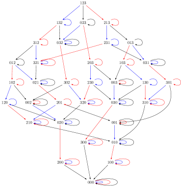
|
We first notice an important difference: on the contrary to the right order is not graded. This has been already noted for . Indeed in the left part of Figure 4.1 we see two paths from to namely on the left and on the right. Starting with the right order is moreover not isomorphic to its dual order.
4.1 -triviality of
In this section we study the right Cayley graph of showing that except for loops (edge from a vertex to itself) it is acyclic. In monoid theoretic terminology, one says that is -trivial. From Coxeter group point of view, this is the analogue on rook of the (dual) right weak order. Note that the order considered here is different to the (strong) Bruhat order. Its analogue for rook is the subject of [Can and Renner(2012)].
Having shown this acyclicity, we will deduce from the symmetry of the relations of that the left sided Cayley graph is also acyclic. By a standard semigroup theory argument, this will imply that the two-sided Cayley graph is acyclic too, that is that is actually -trivial.
We first recall a combinatorial description of the -order of the -Hecke monoid (or equivalently the dual right-weak order of the symmetric group seen as a Coxeter group) [Björner and Brenti(2005)]. Recall that for two permutations and one has if there exists a sequence with such that . Note that, in accord with the monoid convention and contrary to the Coxeter group convention, the identity is the largest element for this order. An algorithmic way to compare two permutations is to use values inversions (sometimes called co-inversions). We give here a definition which is also valid for rooks:
Definition 4.1.
For a rook , the set of inversions of is defined by
| (4.1) |
It is a subset of , but not all subsets are inversions sets of permutations and of rooks as we will see.
Definition 4.2.
A subset is transitive if and implies .
Here is a characterization of inversions sets:
Lemma 4.3.
Given a set , there exists a permutation such that if and only if and are both transitive. When this holds the permutation is unique.
Proof.
This is a folklore result. To reconstruct from its inversion set, one shows that the relation is a total order, that is a permutation. ∎
Inversion sets allow to characterize the right order:
Lemma 4.4 ([Björner and Brenti(2005)]).
Let , then if and only if .
Proposition 4.5 ([Björner and Brenti(2005)]).
The right -order on permutations is a lattice. The meet of and is characterized by: is the transitive closure of . The join of and is characterized by: is the transitive closure of .
We now present how to adapt inversion sets to rooks. The idea is to record usual inversions as well as inversion with a letter. Here is a way to do it:
Definition 4.6.
We call the support of a rook denoted the set of non-zero letters appearing in its rook vector. For each letter , we denote the number of which appear after in the rook vector of .
We finally say that is the rook triple associated to .
Example 4.7.
For example for , one gets , together with , , and .
Here is a characterization of the rook triples:
Proposition 4.8.
A triple where , and is the rook triple of a rook if and only if the three following properties hold:
-
•
the sets and and are both transitive.
-
•
for , one has ;
-
•
if then else .
Moreover, when these properties hold the corresponding rook is unique.
Proof.
We first prove the direct implication. The first statement says that if one erases the zeros from a rook, one gets a permutation of its support. The second statement says that there are zeros. The third statement says that if is after in , then there are less to the right of than to the right of .
Conversely, given such a triple, we can reconstruct a rook in two steps: the first condition ensures that there is a unique permutation of the support with inversions set . The third statement says that the function is decreasing along the word . As a consequence, writing the subword of composed by the letters such that , one has
| (4.2) |
Note that some of the may be empty. Then the rook
| (4.3) |
is indeed associated with the triple and is by construction unique. ∎
Example 4.9.
Going back to Example 4.7, consider the following triple with :
There is a unique permutation of with inversion set , namely . Writing below for each letter of , we get and see that is indeed decreasing. We then get that , , , , so that we recover .
Our aim is now to show that the -order is actually an order. To do so, we start by defining combinatorially an order , and then show that and are actually equivalent.
Definition 4.10.
Let and . We write if and only if the three following properties hold:
-
•
,
-
•
,
-
•
for .
Remark 4.11.
If and are permutations, then , so that if and only if .
Moreover, as a consequence of the second condition, if and then . We abstract this fact with the following definition and lemma:
Definition 4.12.
Let and . We say that is -compatible if and implies , for all .
The previous remark now rephrases as:
Lemma 4.13.
If then is -compatible.
We will further need the following basic facts about compatibility:
Lemma 4.14.
The union of two -compatibles sets and is -compatible.
If is and -compatible, then it is -compatible.
If is -compatible then it is compatible with the transitive closure of .
We get back to the study of .
Proposition 4.15.
The set endowed with the relation is a poset with maximal element and minimal element .
Proof.
The relation is reflexive, by definition.
If are such that and then and therefore and . As a consequence, the non-zero letters appear in the same order in and and the zeros are in the same places. Thus is antisymmetric.
Let . Then . Let with . Necessarily so that and consequently . Finally if then . Thus is transitive. ∎
Theorem 4.16.
Let Then if and only if .
Proof.
By definition, if there exists such that . Using the identification of Corollary 3.49, this is equivalent to . By abuse of notation in this proof we will therefore write if there exists such that .
For the direct implication, by induction and transitivity, it is sufficient to assume that with and show .
-
•
If . Then . Since we must have and also . If then and . On the contrary, if , then and for and .
-
•
If . Since we have and . We can deduce that . Furthermore,
(4.4) Finally for , .
For the converse implication, assume that . By induction and transitivity it is sufficient to show that there exists such that and . We proceed by a case analysis. First since , we can distinguish whether or . In the equality case, we further distinguish whether or not.
-
•
If , and , then there must exist such that . Pick the leftmost in which verifies this condition. First, there must be some on the left of in because there are on the right and at least in the word. Thus is not the first letter of .
Let be the letter immediately preceding in . We claim that either or is after in . Indeed if and is before in then we have . Moreover because there is no zero in between and . Therefore which contradicts our choice of as being the leftmost.
Now, call the position of this in . If , the only difference between the rook triples of and is that so that . On the contrary, if , then the only difference between the rook triples of and is that so that again .
-
•
If , and , then necessarily . Write and the words obtained by removing the zeros in and . The inclusion of inversions shows that where is the right order for permutations of . As a consequence, we know that it is possible to exchange two consecutive letters in to get a permutation of such that
(4.5) From the equality of , there cannot be any between and in , thus and are consecutive in as well. Writing for the position of in , we have .
-
•
The remaining case is . Let . If is in position in then and we are done in this case.
Otherwise if is not in position , we claim that the letter immediately preceding in is smaller than . If not, then there is an inversion in . Since is -compatible, then . This contradicts our choice of as being the maximum.
Writing for the position of in , we proceed as in the end of the first case: the only difference between the rook triples of and is that so that again . ∎
We are now in position to prove the main result of this section:
Corollary 4.17.
The monoid is -trivial, -trivial and thus -trivial.
4.2 The lattice of the -order
Our goal here is to show that, similarly to the weak order of permutations, the -order for the rooks is a lattice. We start with an algorithm which computes the meet.
Theorem 4.18.
Let and be two rooks of size . Define a new rook by the following algorithm:
-
•
Let be the transitive closure of .
-
•
Let be the largest (for inclusion) -compatible set contained in .
-
•
Let .
-
•
Finally, for let with the convention that if .
Then is a rook triple whose associated rook is the meet of and for the -order.
Proof.
We first prove that is indeed a rook triple.
-
•
By definition, , let us show that and are transitive. We claim that is the transitive closure of . Indeed, for any , then . By definition of the transitive closure, there exists a decreasing sequence of integer such that for . By induction, since , compatibility ensures that all of the belong to . Hence the claim.
As a consequence, using Proposition 4.5, is the inversion set of the meet in the permutohedron of the restriction of and to so that and are transitive.
-
•
On has . So that the condition holds.
-
•
Write so that . If , the transitivity of ensures that as sets so that . Conversely write . If , the transitivity of shows that implies . By contraposition, implies so that and therefore .
Hence, we have proved that is a rook triple. It remains to prove that its associated rook is the meet . By construction, and . So that we only need to prove that for any rook such that and then .
-
•
Using the rephrasing of Remark 4.11 we know that then is and -compatible and therefore compatible with the transitive closure of their union . Since is defined as the largest such set, .
-
•
Suppose , with . Then by construction of , there is a decreasing sequence such that for . By induction, having and , one prove and . One concludes by transitivity that .
-
•
Finally, assume . Then and . Moreover for any such that , by the preceding item, and . One deduces that and . We just showed that . ∎
Corollary 4.19.
The -order of is a lattice.
Proof.
From the previous theorem, we know that is a meet semi-lattice. Now it is well known that a meet semi-lattice with a maximum element is a lattice. ∎
From the proof, we have a more explicit algorithm to compute the meet:
-
•
Start with . Then while one can find a with and , remove from . When no more such can be found, is the support of .
-
•
Using the usual algorithm for permutations of the set (see the sketch of the proof of Lemma 4.3), compute the meet of the restriction and .
-
•
Compute the function using as in the statement of Theorem 4.18.
-
•
Finish inserting the zeros using as in the proof of Proposition 4.8.
Example 4.20.
Let and . So . But and and . So . We then get , So that . It remains to insert the zeros. One compute and so that . Here is a bigger example: Let us compute . One finds that , and and , so that . Similarly
In the case of permutations, the involution where is the maximal permutation (otherwise said, is the mirror image of ) is an isomorphism from the -order to its dual. A a consequence, one can compute the join using the meet: . However, as seen for example on Figure 4.1 this trick does not work anymore for rooks. This ask for an algorithm to compute the join of two rooks. To describe this algorithm, we need a notion of non-inversion and a dual notion of compatibility:
Definition 4.21.
For any rook , call set of version of the set:
| (4.6) |
Let and . We say that is dual -compatible if and implies .
Theorem 4.22.
Let and be two rooks of size . Define a new rook by the following algorithm:
-
•
Let where is the transitive closure of .
-
•
Let be the smallest dual -compatible set containing .
-
•
Let .
-
•
Finally, for let , with the convention that if .
Then is a rook triple whose associated rook is the join .
The proof is very similar to the one we did for the meet and is left to the reader.
Example 4.23.
Let us compute . One finds , and , so that .
We want to enumerate the join-irreducible elements. As in the classical permutohedron, they are related to descents, however, it the case of rooks, they are two different notions of descents.
Definition 4.24 (Weak and strict descents).
Let be a rook. For any , we say that is a weak (right) descent of if . We say that is a strict (right) descent if there exists a rook such that . Moreover, in the particular case , we say that is a strict descent with multiplicity , if there are exactly rooks such that .
Any strict descent is a weak descent. Indeed if then . Weak descent and strict descents are equivalent when restricted to permutations, but they differ on rooks. For example, the rook , has 3 weak descent namely , but only are strict ( and ) and has multiplicity : .
Lemma 4.25.
The multiplicity of as a strict descent in a rook is if does not start with and is the number of in otherwise.
Definition 4.26.
An element of a lattice is called meet irreducible if it can not be obtained as a non trivial meet that is implies or .
An equivalent definition is that has only one successor in the Hasse diagram of . By definition, in a finite lattice, any element can be written as the meet of some meet irreducible elements. As a consequence, they form the minimal generating set of the meet semi-lattice.
For permutations, the number of meet irreducible for the -order (that is permutation with only one descent) is . It is a particular case of Eulerian numbers and is recorded as OEIS A000295. Here are the first values
| (4.7) |
For rooks, the number of meet irreducibles has a very simple expression too:
Proposition 4.27.
The number of meet irreducibles for is .
This sequence is recorded as OEIS A001047. Here are the first values
| (4.8) |
We will actually prove a stronger statement, the previous one will follow thanks to the identity:
| (4.9) |
Proposition 4.28.
For any rook vector denote the first value if its non zero, and if its zero. The number of meet-irreducibles of such that is .
Proof.
A rook is meet irreducible if and only if it has a unique strict descent (counting multiplicities). Consider a meet irreducible rook with . There are two cases:
-
•
if , then the rook is composed by two nondecreasing sequences, the first one starts with . So each number smaller than , either appears in the second subsequence or, do not appear at all so that the second sequence starts with some . Similarly each number larger than , may appear in any of those two subsequences or not at all. So the number of choices is .
-
•
if , then start either with or . We want to show that the number of such rooks is . We show that the set of those rooks is in bijection with the set of maps .
In the following, for any set of integers we write the word obtained by writing the letter of in increasing order. Given a map , one build a sequence starting with , then ordering the preimage of , putting as many zero as the preimage of , and then ordering the preimage of :
(4.10) By definition, the result is a rook of size with at most one descent. Moreover, each rook with only one descent is obtained exactly once as the image of some .
It remains to show that the maps which give rooks with no descent by the preceding construction are in bijection with rooks having as unique descent with multiplicity . The point is the following: has zero descents, that is is nondecreasing, if and only if there exists a such that
(4.11) If it is the case, we redefine as
(4.12) The set of the rooks obtained this way is the set of increasing rooks which start with a . According to Lemma 4.25, those are exactly the rooks having as unique descent with multiplicity .
On conclude that there are exactly rooks starting either by or . ∎
Example 4.29.
Consider the function . Then which has only one strict descent (the dots are only here to visualize the different part of the right hand side of Equation 4.10).
As a concluding remark on irreducible elements, we note that, on the contrary to permutations, the poset is not self dual. So there is no reason why the number of meet irreducible elements should be equal to the number of join irreducible elements. They indeed differ and we do not have a formula for the number of join irreducibles. We give here the first values:
| (4.13) |
4.3 Chains in the rook lattice
We recall that a chain in a lattice is a sequence of elements such that . A maximal chain is a chain which is not strictly included in another one. Denoting and the minimal and maximal elements of , this is equivalent to , and for every there is no element between and for the order . For the weak order on permutations, maximal chains corresponds to reduced expression of the maximal permutation.
We now consider maximal chains of (thus also by Corollary 3.49). We see in Figure 4.1 that all the maximal chains are not of equal length. Experimental computation of the numbers of maximal chains give the following sequence: . We did not find any nice property: it is not refered in OEIS and the numbers contain big prime factor. A more interesting question is to only consider maximal chains of minimal length, that is reduced expressions of the maximal rook . Note by Lemma 3.4 that . We find the following numbers of such chains:
| (4.14) |
This sequence is refered as OEIS A003121. It counts, among many other things, the number of maximal chains of length (hence maximal) in the Tamari lattice . This suggests that there is a bijection between the chains. It turns out that the coincidence is much stronger: the two posets restricted to the elements appearing in their respective chains of maximal length are isomorphic.
We first need to describe the elements appearing in a reduced expression of . We need the following combinatorial definition for this:
Definition 4.30.
Let be an alphabet and , be two words over . The shuffle product is defined inductively by:
| (4.15) |
the initial condition being that the empty word is the unit element.
Proposition 4.31.
The rook vectors appearing as a left factor of a reduced expression of are the rooks:
| (4.16) |
Proof.
Let as defined by Equation 4.16. We assume that has zeros, so that the nonzero letters appearing in are . Take the reduced expression for given by the -code (Definition 3.34). Since the nonzero letters are in order, this expression if of length . In order to bring to by right action we repeat the following steps until we reach : let be the first nonzero letter and its position. Then multiplying on the right by brings to the front and kills it. The length of the word for obtained this way is equal to
| (4.17) |
This is the length of , hence the expression is reduced, and appears in a maximal chain of minimal length.
Now we prove the converse inclusion by contradiction. Let , with zeros. We want to show that there is no reduced word for of the form where is a word for . Assume that we have such a word. Since , then either there is a nonzero letter before a nonzero letter with , or there is a nonzero letter while a letter is missing. The algorithm computing the canonical reduced word (Definition 3.34) shows that:
| (4.18) |
We call the rook vector obtained from by replacing the nonzero letters by in this order, so that . Then gives as well. Thus . So that , which is absurd. ∎
In particular note that:
Example 4.32.
We now introduce a sequence of bijections from to some special Dyck paths, that is vertices of the Tamari lattice. For now, recall that a Dyck path of length is a path in the plane starting from , ending in made with north-east (NE) and south-east (SE) such that the path is always above the line . We represent a Dyck path by a word of size with letters and letters , where is a SE step, and a NE step, and such that in every prefix of the word the number of is less or equal to the number of . For instance is a Dyck path. We will also represent it .
The first bijection sends an element of to a subset of the following way:
| (4.19) |
This application is clearly a bijection since the nonzero letters of are in this order, where is the number of zeros of . Now that we have a subset of we can use the bijection to compositions of introduced in Equation 2.5. If the actions of the generators of through the bijection are as follows:
| (4.20) | |||||
| (4.21) |
We finally send a composition of to a Dyck path as follows:
| (4.22) |
It is easy to check that the Dyck paths we obtain this way are exactly those for whose the pattern is forbidden. Note that the action of the generators of is thus to replace a by which pictorially inserts a diamond in a “valley”. See Figure 4.2. We say that a Dyck path contains another Dyck path , and we denote it , if the path is above the path . Then the -order on is mapped to the order on Dyck paths avoiding the pattern by the bijection . The maximal element of the poset on Dyck path is and its minimal . See the first line of Figure 4.5 to see all these isomorphisms. We finally remark that all these posets are actually lattices.
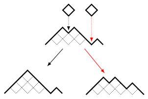
Now we briefly present the Tamari order, the reader should ref to [Tamari(1962)] for more details. A Dyck path is called primitive if it is not empty and has no other contact with the line except at the starting and ending point. If is a Dyck path such that has a SE step followed by a primitive path . Then the rotation on is to exchange the SE step with the primitive path . See Figure 4.3. These rotations are the cover relations of the Tamari order .
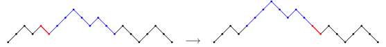
We are interested in Dyck paths in a maximal chain of length in the Tamari lattice of size . We denote by their set.
Proposition 4.33.
The set is exactly the set of Dyck paths avoiding . Furthermore the order restricted to is equal to the order of inclusion .
Proof.
The difference of diamonds between the minimal element and the maximal element is exactly , so that each rotation must add only one diamond. But a rotation on a SE step followed by two NE steps adds at least two diamonds, so that we can not rotate in such a SE step. Moreover the rotations on another licit SE step preserve the pattern, so that an element with pattern can not be in . On the contrary if is a Dyck path avoiding , then a rotation is exactly to add a diamond in a valley, and the resulting Dyck path also avoids .
Now that we have the description of elements of , doing a rotation corresponds to adding a diamond on a valley, so that the order implies the order . Furthermore, by definition of the order , the converse also holds. ∎
As a consequence we have proven that the order on obtained through the bijection is exactly the Tamari order, so that the posets of and are isomorphic.
The elements appearing in appears in many different contexts, see [Hohlweg and Lange(2007), Hohlweg et al.(2011)Hohlweg, Lange, and Thomas, Labbé and Lange(2018)] and the references in the latters. They correspond to binary trees which are chains, that is also binary trees with exactly one linear extension. For this reason they are called singletons. Equivalently they are permutations avoiding the patterns and , or permutations with exactly one element in their sylvester class, that is common vertices between the associahedron and the permutahedron. Furthemore the historic definition of the associahedron is to keep only the faces of the permutahedron which contains such a singleton. See Figure 4.4, and [Hohlweg and Lange(2007)] for more details. See also Figure 4.5 for all the bijections seen in this section.
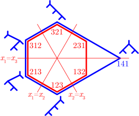
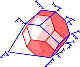
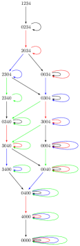
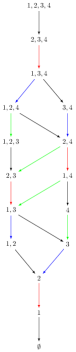

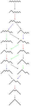
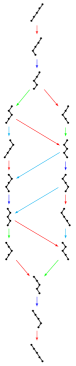
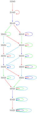
4.4 Geometrical remarks
Recall that the right Cayley graph of the symmetric group is the -skeleton of a polytope namely the permutohedron [Ziegler(1995), Example 0.10]. It is defined as the convex hull of the set of points whose coordinates are permutations. It therefore lives in the hyperplane , so that it is a polytope of dimension .
Starting with , we can not hope that the right Cayley graph of could be the -skeleton of a polytope. Indeed in the element is always of degree , being linked only to and , whereas the identity is of degre . Thus it is impossible to get a polytope.
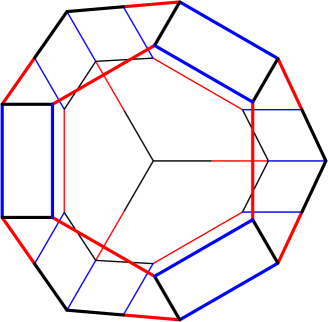
Nevertheless, one can consider in a -dimensional space the set of points whose coordinates are rook vectors (see Figure 4.6). The extremal points of its convex hull are the points in
| (4.23) |
This polyedron appeared under the name of stellohedron in [Manneville and Pilaud(2017), Figure 18] where it was defined as the graph associahedron of a star graph. It is also the secondary polytope of (see [Gelfand et al.(2008)Gelfand, Kapranov, and Zelevinsky]), two concentric copies of a -dimensional simplex, which can also be defined as
| (4.24) |
So we can see the Cayley graph of as being drawn on the face of the stellohedron. One can recover this graph from the permutohedron by taking all its projections on coordinate planes. Indeed, it is just saying that a rook can be obtained from a permutation replacing some entries by zeros and that edges are mapped to an identical edge or contracted.
4.5 A monoid associated to the stellohedron
The geometrical considerations raise the question whether there is a monoid structure giving the skeleton of the Stellohedron as Cayley graph. It turns out that the answer is true. Will we show moreover that there are monoids and lattice structures on graphs interpolating between the rook case and the stellar case.
Definition 4.34.
For any rook denote define to be the rook obtained by replacing by all the letter smaller that in .
Example 4.35.
and thus . Similarly and thus .
Clearly for any rook then , and for any one has . We have then proved the following lemma:
Lemma 4.36.
The map is a projection (i.e. ) on .
Proposition 4.37.
Denote the map corresponding to in , that is . Then is compatible with the product of , namely for any
| (4.25) |
As a consequence, there is a unique monoid structure on such that such that is a surjective monoid morphism.
Proof.
We now explicit the left and right multiplication of the generator in :
Proposition 4.38.
We denote . Then is generated by . And for and , one has and where is the vector obtained by replacing all the element less or equal to by in .
On the left, the product is given by if and and in all the other cases.
We can moreover give a presentation for this new monoid:
Theorem 4.39.
The stellar monoid is the quotient of the rook monoid by the relations
| (ST) |
for .
In order to prove the theorem, we need two preliminary lemmas.
Lemma 4.40.
Relation ST holds in .
Proof.
If we apply both side of Relation ST on the left on the identity rook, then exchange and and kills all letters from to . So both side are equal. ∎
Lemma 4.41.
Proof.
Proof of Theorem 4.39.
From Corollary 3.49, for any rook , its -code verifies (with the notation of Definition 3.34):
| (4.27) |
We denote with the convention that if all the are positive. Then thanks to relation ST’ we know that
| (4.28) |
where the first column is empty if . We call stellar canonical word any word appearing on the right hand side of this equation. In this case, the verify , so that there are
| (4.29) |
stellar canonical words. We have shown that each rook is congruent to a stellar canonical words modulo ST and that they are as many stellar canonical words as element of . As a consequence Relation ST is the only relations needed to get from . ∎
4.5.1 The stelloid lattice
By analogy to the Rook lattice, we might wonder if the -order or -order of are lattices (on the contrary to rooks, they are not isomorphic). It turns out that the -order is a lattice. See Figure 4.7 for a picture.
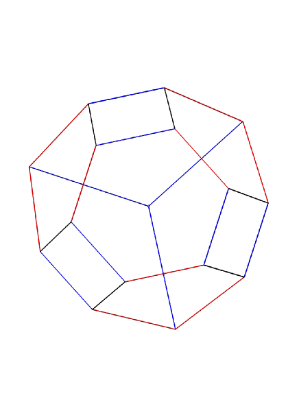
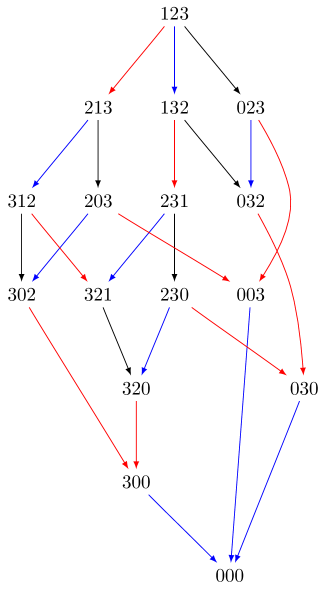
We will show actually a stronger result:
Theorem 4.42.
The -order on is a sublattice of the -order of .
Proof.
We need to conjugate all the rooks to pass to the left order. The conjugate of a stellar rook is a rook such that all the zeroes are at the beginning. Equivalently this means that in its rook triple , the function is the zero function. Now looking at the algorithm for computing the meet and join of two rooks, we have that
| (4.30) | ||||
| (4.31) |
As a consequence both and are zero functions so that and are conjugate stellar rooks too. ∎
Remark 4.43.
The preimage of the stellar rook is which is not a interval of the -order. As a consequence, can’t be a lattice morphism and the -order of is a not a lattice quotient of the -order of .
4.5.2 Higher order Stelloid monoid and lattices
The proofs of the two previous theorem makes it clear that the monoid together with its -lattice is a particular case of a more general construction: for , define the map from rooks to rooks which replace by all the letter such that there is or more missing letter larger that (the usual map is the case ). For example and . Also, . So that for all , we have the inclusion of sets:
| (4.32) |
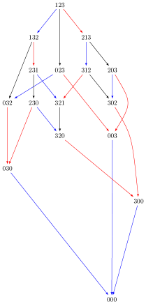
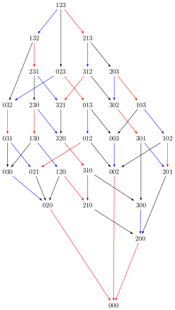
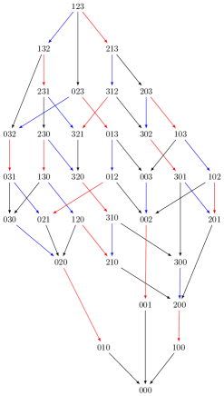
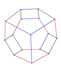
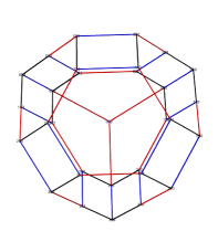
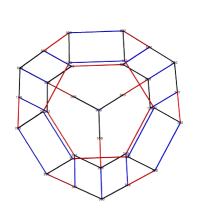
The following array give the cardinality of .
Then the proof of Proposition 4.37 and Theorem 4.42 generalize to this new cases:
Theorem 4.44.
Denote the map corresponding to in . Then this map is a surjective monoid morphism to . Moreover, the -order of is a sublattice of the -order of .
Hence Equation 4.32 is actually a sequence of inclusion of lattices. It also give rise to the following sequence of monoid morphisms:
| (4.33) |
Figure 4.8 shows the three consecutive quotients of together with their geometric counterpart.
We finally remark that the quotient morphism are in the opposite direction of the inclusion of lattices of Equation 4.32. This suggest some kind of duality, but we haven’t been able to give a formulation.
5 Representation theory of the -Rook monoid
The goal of this section is to investigate the representation theory of . We write the monoid algebra of . In the sequel of the article will rather be denoted by . Moreover, will usually denote an element of . Also, we know from Corollary 3.49 and Proposition 3.59 that for any there is a unique rook such that . So when there is a need to distinguish, we will denote in normal letter the elements of the monoid and in boldface as their associated rooks.
We start by summarizing the main results (in particular Corollary 3.49) of the Section 3 which concerns the representations:
Proposition 5.1.
The maps
extended by linearity, are two isomorphisms of representations of between the left and right regular representations and the natural one (acting on ).
5.1 Idempotents and Simple modules
As for any algebra, the representation theory of (or equivalently ) is largely governed by its idempotents, however since is a -trivial monoid, as shown in [Denton et al.(2010/11)Denton, Hivert, Schilling, and Thiéry], it is sufficient to look for idempotents in the monoid itself.
Proposition 5.2.
For any , we denote the zero of the so-called parabolic submonoid generated by .
Proof.
This submonoid is finite since the ambient monoid is finite. By Proposition 4.17 it contains a unique minimal element for the -order, which is a zero. ∎
Proposition 5.3.
For any , write its complement and its associated extended composition. Then where is the block diagonal rook matrix of size whose block are anti diagonal matrices of of size , except the first block which is a zero matrix.
Note that if then the first part of is zero, so that the first zero block is of size and therefore vanishes.
Example 5.4.
If and . Then so that . Similarly, if , then so that . Therefore the associated matrices are:
Proof.
We fix some and consider the associated rook matrix. The block diagonal structure ensures that belongs to the parabolic submonoid . Indeed, suppose that there is a reduced word for with some . Recall, that from Corollary 3.49, this means that . Choose the smallest such . There are two cases whether or not.
-
•
if with , then when computing , the action of will be to kill a column. In this case, the killed column will never appear again so that there is no way to get the correct matrix.
-
•
if with , when computing , the action of is to exchange two columns from two different blocks. However, acting by any will never exchange those two columns again, so that it is not possible to get them back in the correct order.
Hence, we have proven that only contains with that is . Furthermore, using the action on matrices one sees that or equivalently that if and only if . This shows that is the zero of . ∎
Remark 5.5.
If we decompose the set into its maximal components of consecutive letters , then where the product commutes. Moreover, if then where is the size of the first block.
During the proof, we got the following Lemma:
Lemma 5.6.
Let . Then if , and and otherwise.
Proposition 5.7.
The monoid has exactly idempotents: these are the zeros of every parabolic submonoid.
Proof.
We already know that has at least idempotents. We now have to prove this exhaust the idempotents of .
Let an idempotent of . Recall that is the set of the with appearing in any reduced word of . Let us show that , that is the zero of the parabolic submonoid . Indeed for , one can write for some and in . By definition of the -order, this means that . Using [Denton et al.(2010/11)Denton, Hivert, Schilling, and Thiéry, Lemma 3.6], this is equivalent to and to , so that is stable under all its support. ∎
Theorem 5.8.
The monoid has left (and right) simple modules, all one-dimensional, indexed by the subsets of . Let . Its associated simple module is the one-dimensional module generated by with the following action of generators:
| (5.1) |
Proof.
We apply [Denton et al.(2010/11)Denton, Hivert, Schilling, and Thiéry, Proposition 3.1] using Lemma 5.6. ∎
Recall that we write any sufficiently large power of which becomes idempotent, and that the star product of two idempotents is defined as . This endows the set of idempotents with a structure of a lattice where is the meet [Denton et al.(2010/11)Denton, Hivert, Schilling, and Thiéry, Theorem 3.4]. We now explicitely describe this lattice:
Proposition 5.9.
Let . Then .
Proof.
First we note that is inside the parabolic . It is enough to show that it is a zero of this submonoid, and then conclude by unicity. The product formual is is a consequence of [Denton et al.(2010/11)Denton, Hivert, Schilling, and Thiéry, Lemma 3.6]. ∎
Corollary 5.10.
The quotient is isomorphic to the algebra of the lattice of the -dimensionnal cube.
5.2 Indecomposable projective modules
Recall that the indecomposable projective -modules are spanned by descent classes (see Section 2.5 and reference therein for more details). Extending the definition from the Hecke monoid, we define left and right -descents sets of a rook as:
| (5.2) |
Example 5.11.
Let . We have , and the first letter is . So .
Notation 5.12.
We choose to represent an element by a ribbon notation the usual way, with the difference that two zeros are vertical and not horizontal: and not .
This change of convention compared to e.g. [Krob and Thibon(1997)] is due to our choice of taking the ’s and not the ’s for generators of the Hecke algebra. As a consequence, the eigenvalues and are exchanged.
For example, is represented by the ribbon Figure 5.1 shows the ribbon together with their associated descent sets. Figure 5.2 depicts the associated boolean lattice.
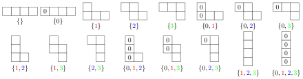

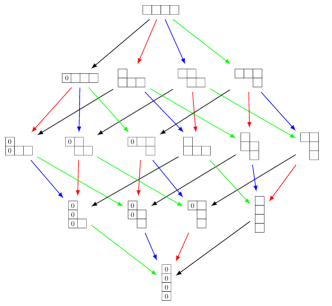
With this notation we can easily find the idempotents of each -descent set:
Proposition 5.13.
In each -descent class there is a unique idempotent. It is obtained by filling ribbon shape by numbers to in this order, going through the columns left to right and bottom to up. Then if is in the descent class, fill the first column with zeros.
Proof.
Example 5.14.
Consider the -descent set in size . We show below its associated ribbon shape and its idempotent
We now follow [Denton et al.(2010/11)Denton, Hivert, Schilling, and Thiéry, Section 3.4], specializing it to the combinatorics of . Recall that the automorphism sub-monoid and are defined by
| (5.3) |
Proposition 5.15.
Let .
| (5.4) |
Proof.
We do the proof for . The first inclusion is clear.
Let . So . Assume that . Let a reduced expression of . Let be the smallest index such that . Then by minimality. Since , and by -triviality we get . This contradict the minimality. ∎
From [Denton et al.(2010/11)Denton, Hivert, Schilling, and Thiéry, Proposition 3.16], we get the following corollary:
Corollary 5.16.
Let
| (5.5) |
Then, applying Theorem 2.10, we get:
Theorem 5.17.
The indecomposable projective -modules are indexed by the -descents sets and isomorphic to the quotient of the associated -descent class by the finer -descent classes.

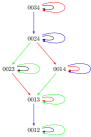
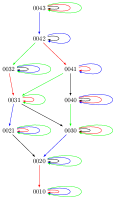
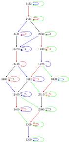
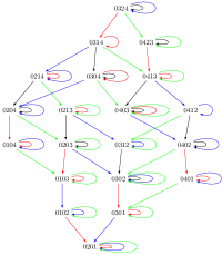
Finally [Denton et al.(2010/11)Denton, Hivert, Schilling, and Thiéry, Theorem 3.20] gives the coefficients of the Cartan matrix of as the number of rooks with a given left and right descent set. We give it in Annex B, for .
Remark 5.18.
Contrary to the classical case [Krob and Thibon(1997)] these quotients are not intervals of the -order: the descent class depicted in Figure 5.4 has two bottom elements.

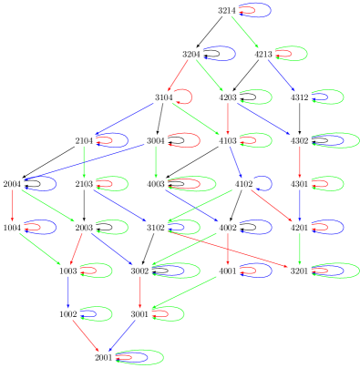
5.3 Ext-Quivers
The Ext-quiver of were first computed in [Duchamp et al.(2002)Duchamp, Hivert, and Thibon] in type , and later in [Fayers(2005)] in the other types. Moreover, [Denton et al.(2010/11)Denton, Hivert, Schilling, and Thiéry] describes an algorithm to compute the quiver of any -trivial monoid. This algorithm is implemented in sage-semigroups from the second author, Franco Saliola and Nicolas M. Thiéry [Hivert et al.(2012–2018)Hivert, Saliola, and Thiéry]. It turns out that the quiver of rook monoids are not different from -Hecke monoids:
Theorem 5.19.
The kernel of the two following algebra morphisms
| (5.6) |
are included in the square radical of their respective domains. As a consequence, these three algebras share the same quiver.
Proof.
Recall that all of these algebras are monoid algebras of -trivial monoids. Thanks to [Denton et al.(2010/11)Denton, Hivert, Schilling, and Thiéry, Corollary 3.8], their radical is generated by commutators. Therefore, the following non zero elements: and lie in the radical of each of these three algebras. The first map has for kernel the ideal generated by the relation
which thus lies in the square radical. Similarly the kernel of the second map is the ideal generated by
We refer the reader who want to see actual picture of the quiver to [Duchamp et al.(2002)Duchamp, Hivert, and Thibon]. Except for trivial cases, they are not of known type so that the representation theory of starting from is wild.
5.4 Restriction functor to
We now further examine the links between representations of and . Indeed, since is a submonoid of , it acts by multiplication on . We can see as an -module. Moreover, we can transport modules back and between and trough the induction and restriction functors.
We first look at simple modules whose restriction rule is immediate:
Proposition 5.20.
Let , with associated simple -module . Then:
| (5.7) |
where is the simple -module generated by the parabolic .
The rule of induction for simple -modules to -modules is otherwise quite intricate and would be very technical. It would be very similar to what we will do in section 5.5.1 for the induction of simple modules of to another , which is already very technical.
We now look at indecomposable -projective modules.
Proposition 5.21.
Let and the associated indecomposable -projective module. Then:
| (5.8) |
Proof.
This is a consequence of Proposition 5.20, thanks to Frobenius reciprocity (see e.g. [Curtis and Reiner(1990)]). Indeed, since the simple module is the quotient of the indecomposable projective by its radical, the multiplicity of in a projective module is equal to . By Frobenius reciprocity,
| (5.9) |
Now, Proposition 5.20 says that this dimension is only if , otherwise it is . ∎
The restriction of projective modules from to is much more interesting. We will show that -projective modules are still projective when restricted to , and give a precise combinatorial rule.
Definition 5.22.
Let of size , and . We define to be the rook obtained by removing the first entries of and inserting zeros in positions indexed by the elements of .
We also denote the map which takes a rook, put all zeros at the beginning of the word and replace them by the missing letters in decreasing order.
Example 5.23.
For instance and .
For the next results, we will consider to be a left -module by left multiplication. Thus the action is on values as in Definition 3.56.
Theorem 5.24.
is projective over . As a consequence any projective -module remains projective when restricted to .
Proof.
The main remark is that according to Definition 3.56, the left action of for on any rook does not change the zeros: they remain at the same positions and no one are added.
For any , let the set of rooks with zeros in the positions indexed by . Since the action of does not move zeros, we have the following decomposition in -modules:
| (5.10) |
It is enough to prove that each summand are projective since direct sums of projective modules are projective.
For such a summand where zeros are in positions , the linearization of the map of Definition 5.22 is an injective -module morphism. Its image is the set of permutations which start with descents which is a well known projective -module. Indeed, it is the -module generated by the element . This element is the zero of the parabolic submonoid generated by , hence idempotent. Consequently it generates a projective modules. This shows that is projective on . ∎
We now describe explicitely the restriction functor. Recall from Equation 2.8 that the induction product of two indecomposable projective -Module (resp. -Module) and is given by .
Definition 5.25.
Let be an extended composition of . A zero-filling of is a ribbon of shape with boxes either empty, either with inside according to the following rules:
-
•
In the first column, either every box contains if , or none otherwise.
-
•
Outside of the first column, if a box contains then there is no box on its left, and all the boxes below in the same column also contain zeros.
To each of these fillings we associate a tuple of ribbon as follows
-
•
the first entry of the tuple is a column whose size is the total number of zeros in
-
•
the other entries of the tuple are the (down-right) connected components of where the boxes containing a in are removed.
To each splitting, it therefore makes sense to consider the -product .
Example 5.26.
The following picture shows an extended composition followed by some of its -fillings. There are of them.
We now consider two particular -fillings and show the ribbons appearing in the associated respective products (the colors are just to show what happens of each box):
Theorem 5.27.
The indecomposable projective -module associated to an extended composition splits as a -module as
| (5.11) |
where the direct sum spans along all the zero-fillings of , and the product is for the induction product .
Before giving a proof, we give a full example.
Example 5.28.
We decompose restriction of the indecomposable projective -module into indecomposable projective -modules. The colors indicate the different products of zero-filling. Figure 5.5 depict the action of the generators.
Proof.
Let be an indecomposable projective -module and look at it inside the regular representation. We proceed as in the proof of Theorem 5.24: we cut according to the positions of zeros, which comes down to cutting along the zero-fillings. Indeed the conditions of zero-fillings give us only valid fillings, because they still have the good descent set. Moreover, we see all of them appearing in the descent class: for a given zero-filling , we fill the diagram of column after column, left to right, down to up, by the entries starting from the number of zeros in the zero-filling plus to . We get a rook of descent set with zero in the positions given by .
Let be a zero-filling of shape with zeros in positions indexed by elements of . Let be the associated -projective indecomposable module. We consider the restriction . We need to describe the image of . First they start with descents including zeros. We consider the connected components of : the letters at these positions are moved to the right by , but keep their relative order. It is only between the connected components that we can have either a rise or a descent. Then we are getting a subset from a product associated to . And we get them all: take one of them, and fill it with the same rule as before; one gets a permutation and then apply defined in 5.22 to get an element with the good descent set and positions of zeros which will be sent by to an element of the product. ∎
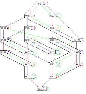

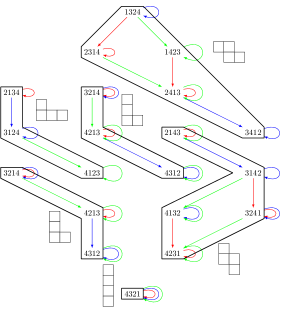
In Annex B, we give the decomposition functor from to for .
We can be a little more precise:
Proposition 5.29.
Let be an indecomposable projective module of . Write its decomposition into indecomposable -projective modules. Then the isomorphism of -module is triangular: with defined in 5.22 and the zero-set linked to .
Proof.
We consider a indecomposable projective , pick a and denote as in the proof of Theorem 5.27 the submodule of rooks whose zeros are in positions indexed by the elements of . The setwise map extends linearly to an isomorphism to the projective but not necessarily indecomposable permutation module . Using [Denton et al.(2010/11)Denton, Hivert, Schilling, and Thiéry, Theorem 3.11 and Corollary 3.19], we know that the basis change decomposing this module to its indecomposable component is uni-triangular. The statement follows by inverting this map. ∎
5.5 Tower of monoids
The goal of this section is to investigate if the chain of submonoids
| (5.12) |
can be endowed with a structure of a tower of monoids [Bergeron and Li(2009)].
Recall that an associative tower of monoids is a sequence where together with a collection of monoid morphisms such that the product defined on the disjoint union is associative.
Proposition 5.31.
The maps
| (5.13) |
defines an associative tower of monoids.
Notation 5.32.
If and we denote .
Furthermore, if is a word on nonnegative integers, denotes the word where all nonzero entries have been increased by .
Proof.
We first show that are morphisms. Let et . Then, by relation of commutation and absorption we get .
The proof of the associativity rely on the following lemma:
Lemma 5.33.
Let and . Then
| (5.14) |
Proof.
Indeed . If then does not appear in any reduced expression of , thus the reduced expressions of and contain generators which do not act on on the same positions. Otherwise appear in , and since all elements of commute with those of , absorbs all the . ∎
We now can compute explicitely the products and , do the four cases whether or not and and check associativity. ∎
Remark 5.34.
The embedding is not injective since , and with : by Lemma 5.33. So we do not have a tower of monoid in the sense of [Bergeron and Li(2009)].
Remark 5.35.
To map to , Remark 3.10 prevents us to use the trivial map : it is not a monoid morphism.
5.5.1 Restriction and induction of simple modules
The goal of this section is to describe the restriction and induction rule of the tower of the -rook monoids. Recall that for , this gives the multiplication and comultiplication rule of the Hopf algebra of quasi-symmetric functions in the fundamental basis [Krob and Thibon(1997)].
Restriction of simples modules
Theorem 5.36.
Let a parabolic of . Then:
| (5.15) |
where .
Proof.
We know that , and that if , and otherwise. The action of on gives us . The generators of act as . It remains only to see how acts on . By Lemma 3.4 we have that . So if there is with , thus . Otherwise, for all , and so . ∎
Induction of simple modules
We can compute the induction of simple module thanks to Virmaux [Virmaux(2014), Theorem 4.3], which we reformulate in our context here. The comparisons are done with the -order in , which we described in Theorem 4.16.
Theorem 5.37 ([Virmaux(2014), Theorem 4.3]).
If and , then
| (5.16) |
where is the set of elements of strictly smaller than , and those of strictly smaller than .
Notation 5.38.
In Equation 5.16, we will denote by the right hand side of the equality. It is a -module. It is also a quotient which is compatible with the canonical basis. By abuse of language, we will say that an element remains in and write if is not mapped to zero in the quotient.
Our first goal is to rephrase Theorem 5.37 in a more combinatorial way.
Notation 5.39.
Until now, we used the notation to design the idempotent of the parabolic submonoid associated to in . In order to avoid confusion, we will now denote it by . Note that as long as , then and have the same reduced expressions and thus the same action of the first -letters on the identity of size .
In the sequel of this section, we fix and . They encode the data of two simple modules of and respectively, or equivalently of two idempotents. We denote and these two idempotents.
Before giving the induction of the simple modules, we go for a serie of lemmas.
Lemma 5.40.
The image of in is the element of associated to if and to otherwise. In particular we have the following cases:
-
•
If then .
-
•
If and then .
-
•
If and then .
Proof.
It is straightforward application of Lemma 5.33. ∎
Remark 5.41.
Note that because of the form of idempotents, .
Lemma 5.42.
Assume that and . Then .
Proof.
We are now considering cases where , writing .
Lemma 5.43.
Assume . Let be an element of which does not vanish in the quotient . Let and be two letters of , not both zero. If and appear both in (resp. and appear both in ) then they appear in in the same order as in (resp. ). Furthermore, all the nonzero letters of appear in . Finally, if is not in then is not in , for all .
Example 5.44.
If and then neither , or , or remain in , respectively because of the first, second and third rule.
Proof.
For the first point, it is sufficient to do the proof when the two letters are consecutive in . Let . So . Assume with and non both zero, and both present in .
Suppose first that , so that and since . Since we deduce that is before in .
Otherwise, . Let be the position of in . So . Then . Also . Thus, while . Since we get . Assume that is left to in . In this case we have , so , the latter being an element by which we quotient in . It is a contradiction.
The proof is the same when and both come from once decreased. The only change are that both letter are nonzero, and that we have to decrease by .
Let us prove the second point by contradiction, assuming that a nonzero letter in is not in . We first show that the first nonzero letter of , say , is not in either. By contradiction, assume that . If then has descent . So must also have it since and , but it is not the case since , which is a contradiction. Otherwise . Since and , and that the generator can only delete the first letter, is in the -order between and a rook in which is there and is in first position. Because of the first point, this element has been sent to in the quotient, and thus which is below as well. So , again this is a contradiction.
The same argument also apply to the third case, with some minor adaptation.
Thus if there is a nonzero letter of lacking in , the first one at least is lacking. We now look at . If , begins with . Then is an element by which we quotient. We have and so , thus , and we get a contradiction.
Otherwise so . We denote by the position of the last and is an element by which we quotient. Since , is in the -order between and a rook in which is there in first position. In particular in , we have a right to . So and , so and thus , for a final contradiction. ∎
Remark 5.45.
Let and the associated idempotent (hence ). We write . Because of Proposition 5.13 we have that if then , , …, and . Furthermore (since ) and .
We are now in position to state the formula giving the induction of simple modules. Recall that denote the so-called shuffle product introduced in Definition 4.30. We also denote the word with letters .
Theorem 5.46.
For , we fix and . Denoting and , the induction of simple modules and is given by
-
1.
If and then .
-
2.
If and then .
-
3.
If and then .
-
4.
If and , , let be the first letter of . Then:
(5.17) -
5.
If and , let be the first letter of . Then
(5.18)
Proof.
-
1.
This case follows directly from Lemma 5.42.
- 2.
-
3.
Since then and . Let . Clearly . We know that has the same number of zeros than and also that its inversions are those of increased by . We deduce that is not below in the -order for . Thus .
-
4.
Denote and let . The same argument than the third point shows that .
Conversely, let . Since (or equivalently, ) Lemma 5.43 tells us that the eventual new zeros of are before the nonzero letters of . By the same lemma, the letters of disappear in the same order than in . So that we have proven:
(5.21) We recall that . We have to show that elements of are not in . A first immediate remark is that all these elements are below . But . Thus, since (by Remark 5.45), in , and so all also, hence the result.
-
5.
Denote Let . The argument of the third point proves that .
Conversely, for , the argument of the fourth point shows that .∎
Recall that the corresponding rule for is the multiplication of the fundamental basis of quasi-symmetric function [Krob and Thibon(1997)]. This rule can be computed as follows [Gessel(1984), Duchamp et al.(2002)Duchamp, Hivert, and Thibon]. Let and be two compositions. Choose any permutation whose descent composition is , for example whose corresponding element is idempotent, and such that . Then
| (5.22) |
As explained by Virmaux [Virmaux(2014)] this is a direct consequence of Theorem 5.37.
To get the analogue of the product of quasi-symmetric functions, one has to use the Theorem 5.46 and then get the projection of the induced module in the Grothendieck ring. This amounts to compute the -descent of every rook vector appearing in the sum according to Jordan-Hölder’s theorem.
Example 5.47.
If , , and . Then and . Theorem 5.46 says that
This gives the following -descent classes:
| Element | ||||||||||
|---|---|---|---|---|---|---|---|---|---|---|
| Descents | 0,1,3 | 0,2 | 0,2,3 | 0,2,4 | 1,2 | 1,3 | 1,4 | 1,2,3 | 1,2,4 | 1,3,4 |
Finally:
Example 5.48.
If , , and . Then and . Theorem 5.46 says that
Then:
| Element | ||||||||
|---|---|---|---|---|---|---|---|---|
| Descents | 0,1,3,4 | 0,1,4 | 0,1,3 | 0,2,4 | 0,2 | 0,2,3 | 1,2,4 | 1,2 |
| Element | ||||||||
| Descents | 1,3 | 1,2,3 | 0,1,2,4 | 0,1,2 | 0,1,3 | 0,2,3 | 1,2,3 | 0,1,2,3 |
This defines the left (resp. right) dual branching graph, where the arrows are labelled by the multiplicity of in the induction of along the morphism (resp. ). The beginning of those two graphs are illustrated in Figures 5.6 and 5.7.
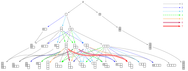
|
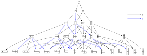
|
Hopf algebra
On the contrary to , we do not get a Hopf algebra. Indeed, the following diagram that express the compatibility of the product with the co-product does not commute:
Here is a counter example: Using Theorem 5.46, we get and . Then
| (5.23) | ||||
Hence this sum has elements, with multiplicity. On the other hand, we saw in Example 5.48 that is a sum of elements (with multiplicity) and Theorem 5.36 shows that the multiplicity does not change by restriction. Hence the result is false.
Induction with
One can wonder what would happen if we rather consider the induction and restriction along the inclusion . It is not a tower of monoids, but the morphisms are injective. We just give the result of the induction of simple modules:
Theorem 5.49.
For , let and . Denoting and , the induction of simple modules and is given by
-
1.
If , let be the first letter of . Then:
(5.24) where the last term begins with letters .
-
2.
If , let be the first letter of . Then
(5.25) where the last term begins with letters .
Proof.
This is a consequence of Theorem 5.46. ∎
5.5.2 Projective indecomposable modules
Restriction of indecomposable projective modules
In order to get a co-product on the Grothendieck ring of projective modules, , we need that is projective over . Unfortunately, this is not the case. We will moreover give counterexamples to the fact that is projective over for both embedding and . This forbids to have any analogues of Bratelli diagrams for projective modules.
Let us take . We want to restrict this projective indecomposable module of to .
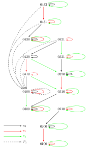
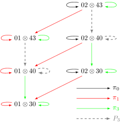
In Figure 5.8 we have on the left the module where we deleted the arrows of and showed the action of . Here we see that has a stable subspace of dimension . On the right we represent what would be a necessary part of the decomposition of , that is . Here we see that (that is the of the right according to the embedding 5.31) as a stable subspace of dimension . Hence it is impossible to cut the left one to get a sum of projective indecomposable modules since the right one must be there and can not be.
We give now two counterexamples which show that it does not work also for the restriction along both embeddings and .
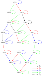
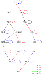
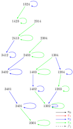
On the left of Figure 5.9 we have the projective module . We see that no element of this module has two zeros, hence send every element to zero. In the middle of the figure we have the same module where we forgot the action of , that is we are looking at the restriction . In the left one we forgot the action of both and but put the action of (none here): we are looking at the restriction along . If the middle and right modules were projective, these figures could be cut as projective modules of . We proceed step by step on the middle one. First we recognise the first chain of five elements which is . Then the element is . All the cycles below with element on top is . The element is again . But the last two elements do not correspond to any projective modules of (it should correspond to since only has the loop of , which is not the case).
We proceed the same way for the right module. We immediatly have a contradiction with the first element which should generate (be careful of the labels!) which is not the case.
As a conclusion of this paragraph, since we do not have the restriction of indecomposable projective modules, we will not be able to have a tower of monoids as for the case of to get NCSF and QSym [Krob and Thibon(1997)].
Induction of indecomposable projective modules
Theorem 5.50.
Let and . Then
Proof.
We reason as in the proof of Proposition 5.21, using Frobenius reciprocity:
| (5.26) |
We are looking for sets such that the simple -module restricts to over . If then and . We conclude considering the two cases whether or not. On the contrary, if then we are in the second case of Theorem 5.36. So either that is , and we have the second case, either it is wrong and in this case no restriction can be obtained. ∎
As we have seen, the natural tower of monoids structure of described here does not have a very nice representation theory. However, this is not the only tower structure, and they may be nice tower structure on their algebras involving linear combination.
Appendix A Implementation
A large part of the algorithms here are implemented in Sagemath [Stein et al.(2018)]. The representation theory where computed using sage_semigroups [Hivert et al.(2012–2018)Hivert, Saliola, and Thiéry] from the second author, F. Saliola and N. Thiéry. The code is freely accessible at
| https://github.com/hivert/Jupyter-Notebooks |
Thanks to the binder technology, one can experiment with it online at
| https://mybinder.org/v2/gh/hivert/Jupyter-Notebooks/master?filepath=rook-0.ipynb |
Appendix B Tables
Decomposition functor
We give the decomposition functor from projective -modules into -modules. They where computed according to Theorem 5.27.
Cartan matrices
We show below the first Cartan matrices of the -rook monoids for . The column on the left shows the associated idempotents.
References
- [Bergeron and Li(2009)] Nantel Bergeron and Huilan Li. Algebraic structures on Grothendieck groups of a tower of algebras. J. Algebra, 321(8):2068–2084, 2009. ISSN 0021-8693. URL https://doi.org/10.1016/j.jalgebra.2008.12.005.
- [Björner and Brenti(2005)] Anders Björner and Francesco Brenti. Combinatorics of Coxeter groups, volume 231 of Graduate Texts in Mathematics. Springer, New York, 2005. ISBN 978-3540-442387; 3-540-44238-3.
- [Butler et al.(2010)Butler, Haglund, Can, and Remmel] Fred Butler, Jim Haglund, Mahir Can, and Jeffrey B. Remmel. Rook theory notes, 2010.
- [Can and Renner(2012)] Mahir Bilen Can and Lex E. Renner. Bruhat-Chevalley order on the rook monoid. Turk J. Math, 36(2):499–519, 2012.
- [Carter(1986)] R. W. Carter. Representation theory of the -Hecke algebra. J. Algebra, 104(1):89–103, 1986. ISSN 0021-8693. URL https://doi.org/10.1016/0021-8693(86)90238-3.
- [Curtis and Reiner(1990)] Charles W. Curtis and Irving Reiner. Methods of representation theory. Vol. I. Wiley Classics Library. John Wiley & Sons, Inc., New York, 1990. ISBN 0-471-52367-4. With applications to finite groups and orders, Reprint of the 1981 original, A Wiley-Interscience Publication.
- [Demazure(1974)] Michel Demazure. Désingularisation des variétés de Schubert généralisées. Ann. Sci. École Norm. Sup. (4), 7:53–88, 1974. ISSN 0012-9593. Collection of articles dedicated to Henri Cartan on the occasion of his 70th birthday, I.
- [Denton(2010)] Tom Denton. A combinatorial formula for orthogonal idempotents in the -Hecke algebra of the symmetric group. 2010. preprint arXiv:1008.2401v1 [math.RT].
- [Denton et al.(2010/11)Denton, Hivert, Schilling, and Thiéry] Tom Denton, Florent Hivert, Anne Schilling, and Nicolas M. Thiéry. On the representation theory of finite -trivial monoids. Sém. Lothar. Combin., 64:Art. B64d, 44, 2010/11. ISSN 1286-4889.
- [Duchamp et al.(2002)Duchamp, Hivert, and Thibon] Gérard Duchamp, Florent Hivert, and Jean-Yves Thibon. Noncommutative symmetric functions. VI. Free quasi-symmetric functions and related algebras. Internat. J. Algebra Comput., 12(5):671–717, 2002. ISSN 0218-1967.
- [Fayers(2005)] Matthew Fayers. 0-Hecke algebras of finite Coxeter groups. J. Pure Appl. Algebra, 199(1-3):27–41, 2005. ISSN 0022-4049. URL https://doi.org/10.1016/j.jpaa.2004.12.001.
- [Flajolet and Sedgewick(2009)] Philippe Flajolet and Robert Sedgewick. Analytic combinatorics. Cambridge University Press, Cambridge, 2009. ISBN 978-0-521-89806-5. doi: 10.1017/CBO9780511801655. URL http://dx.doi.org/10.1017/CBO9780511801655.
- [Ganyushkin and Mazorchuk(2006)] Olexandr Ganyushkin and Volodymyr Mazorchuk. Combinatorics and distributions of partial injections. Australasian J. of Comb., 34:161–186, 2006. ISSN 2202-3518.
- [Gay and Hivert(2018)] Joël Gay and Florent Hivert. The -Renner monoids. page 60, 2018.
- [Gelfand et al.(1995)Gelfand, Krob, Lascoux, Leclerc, Retakh, and Thibon] I.M. Gelfand, D. Krob, A. Lascoux, B. Leclerc, V.S. Retakh, and J.Y. Thibon. Noncommutative symmetrical functions. Advances in Mathematics, 112(2):218 – 348, 1995. ISSN 0001-8708. doi: https://doi.org/10.1006/aima.1995.1032. URL http://www.sciencedirect.com/science/article/pii/S0001870885710328.
- [Gelfand et al.(2008)Gelfand, Kapranov, and Zelevinsky] Israel Gelfand, Mikhail M. Kapranov, and Andrei Zelevinsky. Discriminants, resultants and multidimensional determinants. Mod. Birkhäuser Class. Birkhäuser Boston, 2008.
- [Gessel(1984)] Ira M. Gessel. Multipartite -partitions and inner products of skew Schur functions. In Combinatorics and algebra (Boulder, Colo., 1983), volume 34 of Contemp. Math., pages 289–317. Amer. Math. Soc., Providence, RI, 1984.
- [Green(1951)] J. A. Green. On the structure of semigroups. Ann. of Math. (2), 54:163–172, 1951. ISSN 0003-486X.
- [Guilbaud and Rosenstiehl(1963)] Georges Th. Guilbaud and Pierre Rosenstiehl. Analyse algébrique d’un scrutin. Math. Sci. Hum., 4:9–33, 1963.
- [Halverson(2004)] Tom Halverson. Representations of the -rook monoid. J. Algebra, 273(1):227–251, 2004.
- [Hivert et al.(2012–2018)Hivert, Saliola, and Thiéry] Florent Hivert, Franco Saliola, and Nicolas M. et al. Thiéry. sage-semigroup: A semigroup (representation) theory library for sagemath. https://github.com/nthiery/sage-semigroups/, 2012–2018.
- [Hohlweg and Lange(2007)] Christophe Hohlweg and Carsten E. M. C. Lange. Realizations of the associahedron and cyclohedron. Discrete Comput. Geom., 37(4):517–543, 2007. ISSN 0179-5376. URL https://doi.org/10.1007/s00454-007-1319-6.
- [Hohlweg et al.(2011)Hohlweg, Lange, and Thomas] Christophe Hohlweg, Carsten E. M. C. Lange, and Hugh Thomas. Permutahedra and generalized associahedra. Adv. Math., 226(1):608–640, 2011. ISSN 0001-8708. URL https://doi.org/10.1016/j.aim.2010.07.005.
- [Iwahori(1964)] Nagayoshi Iwahori. On the structure of a Hecke ring of a Chevalley group over a finite field. J. Fac. Sci. Univ. Tokyo Sect. I, 10:215–236 (1964), 1964.
- [Josuat-Vergès(2011)] Matthieu Josuat-Vergès. Rook placements in young diagrams and permutation enumeration. Advances in Applied Mathematics, 47(1):1 – 22, 2011. ISSN 0196-8858. doi: https://doi.org/10.1016/j.aam.2010.04.003. URL http://www.sciencedirect.com/science/article/pii/S0196885810000515.
- [Krob and Thibon(1997)] Daniel Krob and Jean-Yves Thibon. Noncommutative symmetric functions. IV. Quantum linear groups and Hecke algebras at . J. Algebraic Combin., 6(4):339–376, 1997. ISSN 0925-9899. URL https://doi.org/10.1023/A:1008673127310.
- [Labbé and Lange(2018)] Jean-Philippe Labbé and Carsten Lange. Cambrian acyclic domains: counting -singletons, 2018.
- [Lam et al.(2010)Lam, Schilling, and Shimozono] Thomas Lam, Anne Schilling, and Mark Shimozono. -theory Schubert calculus of the affine Grassmannian. Compos. Math., 146(4):811–852, 2010. ISSN 0010-437X. doi: 10.1112/S0010437X09004539.
- [Lascoux(2001)] A. Lascoux. Transition on Grothendieck polynomials. In Physics and combinatorics, 2000 (Nagoya), pages 164–179. World Sci. Publ., River Edge, NJ, 2001.
- [Lascoux(2003)] A. Lascoux. Symmetric Functions and Combinatorial Operators on Polynomials. Number 99 in Conference board of the Mathematical Sciences regional conference series in mathematics. American Mathematical Society, 2003. ISBN 9780821828717. URL https://books.google.de/books?id=RVj6MAAACAAJ.
- [Lascoux and Schützenberger(1987)] A. Lascoux and M. P. Schützenberger. Symmetrization operators on polynomial rings. Functional Analysis and Its Applications, 21(4):324–326, 1987. ISSN 1573-8485. doi: 10.1007/BF01077811. URL https://doi.org/10.1007/BF01077811.
- [Lascoux(2003/04)] Alain Lascoux. Schubert & Grothendieck: un bilan bidécennal. Sém. Lothar. Combin., 50:Art. B50i, 32 pp. (electronic), 2003/04. ISSN 1286-4889.
- [Lothaire(2002)] M. Lothaire. Algebraic Combinatorics on Words. Encyclopedia of Mathematics and its Applications. Cambridge University Press, 2002. doi: 10.1017/CBO9781107326019.
- [Macdonald(1995)] I. G. Macdonald. Symmetric functions and Hall polynomials. Oxford Mathematical Monographs. The Clarendon Press Oxford University Press, New York, second edition, 1995. ISBN 0-19-853489-2. With contributions by A. Zelevinsky, Oxford Science Publications.
- [Manneville and Pilaud(2017)] Thibault Manneville and Vincent Pilaud. Compatibility fans for graphical nested complexes. Journal of Combinatorial Theory, Series A, 150:36 – 107, 2017. ISSN 0097-3165. doi: https://doi.org/10.1016/j.jcta.2017.02.004. URL http://www.sciencedirect.com/science/article/pii/S009731651730016X.
- [Miller(2005)] Ezra Miller. Alternating formulas for -theoretic quiver polynomials. Duke Math. J., 128(1):1–17, 2005. ISSN 0012-7094. doi: 10.1215/S0012-7094-04-12811-8.
- [Mitchell and Torpey(2018)] James d. Mitchell and Michael Torpey. LibSemigroup: A library for semigroups and monoids - version 0.6.3. https://james-d-mitchell.github.io/libsemigroups/, 2018.
- [Norton(1979)] P. N. Norton. -Hecke algebras. J. Austral. Math. Soc. Ser. A, 27(3):337–357, 1979. ISSN 0263-6115.
- [Pin(2010)] Jean-Eric Pin. Mathematical Foundations of Automata Theory. 2010. URL http://www.liafa.jussieu.fr/~jep/MPRI/MPRI.html.
- [Renner(1995)] Lex E. Renner. Analogue of the Bruhat decomposition for algebraic monoids. II. The length function and the trichotomy. J. Algebra, 175(2):697–714, 1995.
- [Riordan(2002)] J. Riordan. Introduction to Combinatorial Analysis. Dover Books on Mathematics. Dover Publications, 2002. ISBN 9780486425368. URL https://books.google.fr/books?id=zWgIPlds29UC.
- [Sloane(2015)] Neil J. A. Sloane. The On-Line Encyclopedia of Integer Sequences Foundation Inc, 2015. URL http://oeis.org.
- [Solomon(1990)] Louis Solomon. The Bruhat decomposition, Tits system and Iwahori ring for the monoid of matrices over a finite field. Geom. Dedicata, 36(1):15–49, 1990.
- [Solomon(2004)] Louis Solomon. The Iwahori algebra of . A presentation and a representation on tensor space. J. Algebra, 273(1):206–226, 2004.
- [Stein et al.(2018)] W. A. Stein et al. Sage Mathematics Software. The Sage Development Team, 2018. URL http://www.sagemath.org.
- [Steinberg(2016)] Benjamin Steinberg. Representation Theory of Finite Monoids. Universitext. Springer, New York, 2016. ISBN 978-3-319-43930-3.
- [Tamari(1962)] Dov Tamari. The algebra of bracketings and their enumeration. Nieuw Arch. Wisk, 3(10):131–146, 1962.
- [Virmaux(2014)] Aladin Virmaux. Partial categorification of hopf algebras and representation theory of towers of -trivial monoids. Proceeding of FPSAC 2014 in DMTCS proc. AT, pages 741–752, 2014.
- [yves Thibon(1998)] Jean yves Thibon. Lectures on noncommutative symmetric functions. 39–94, Math. Soc. Japan Memoirs, 11:39–94, 1998.
- [Ziegler(1995)] Günter M. Ziegler. Lectures on polytopes, volume 152 of Graduate Texts in Mathematics. Springer-Verlag, New York, 1995. ISBN 0-387-94365-X. URL https://doi.org/10.1007/978-1-4613-8431-1.
Joël Gay: E-mail address: joel.gay@lri.fr
Florent Hivert: E-mail address: florent.hivert@lri.fr
Laboratoire de Recherche en Informatique (LRI, UMR CNRS 8623),
Université Paris Sud, Université Paris-Saclay, CNRS,
Bâtiment 650, Université Paris Sud 11, 91405 ORSAY CEDEX, FRANCE.