Bayesian epidemiological modeling
over high-resolution network data

Abstract

Mathematical epidemiological models have a broad use, including both qualitative and quantitative applications. With the increasing availability of data, large-scale quantitative disease spread models can nowadays be formulated. Such models have a great potential, e.g., in risk assessments in public health. Their main challenge is model parameterization given surveillance data, a problem which often limits their practical usage.

We offer a solution to this problem by developing a Bayesian methodology suitable to epidemiological models driven by network data. The greatest difficulty in obtaining a concentrated parameter posterior is the quality of surveillance data; disease measurements are often scarce and carry little information about the parameters. The often overlooked problem of the model’s identifiability therefore needs to be addressed, and we do so using a hierarchy of increasingly realistic known truth experiments.

Our proposed Bayesian approach performs convincingly across all our synthetic tests. From pathogen measurements of shiga toxin-producing Escherichia coli O157 in Swedish cattle, we are able to produce an accurate statistical model of first-principles confronted with data. Within this model we explore the potential of a Bayesian public health framework by assessing the efficiency of disease detection and -intervention scenarios.

Keywords: Bayesian parameter estimation, Pathogen detection, Disease intervention, Synthetic Likelihood, Spatial stochastic models.

1 Introduction

Mathematical and computational modeling are the dominating approaches in the analysis of the dynamics of diseases. The latter approach becomes increasingly important as the amount of relevant data grows. Large-scale computational epidemiological models have been successfully employed to evaluate and inform disease mitigation strategies [17, 18, 21, 9, 33, 7]. With the increasing qualities of data, the possibility of enhancing the resolution through data integration down to the scale of single individuals in a large population has also been realized [13, 18, 4, 32, 7]. In similar spirit, detailed contact data has been used to drive models of disease spread at various population sizes [40, 43, 3, 36, 44, 7]. Data-driven models have aided in an understanding of epidemic outbreaks and endemic conditions on scales and at a level of detail that were not previously possible [18, 3, 54, 29, 51, 7].

Many infectious human diseases have a zoonotic origin, e.g., salmonellosis or infection by shiga toxin-producing Escherichia coli O157 (STEC O157) [14, 15]. Taking a One Health perspective, we argue that to address challenges with existing and emerging threats of zoonotic disease, the aim for computational animal disease models should be to take their place as an integrated part in public health evaluations. This clearly puts high demands on the accuracy and the way any modeling uncertainties are handled. Indeed, an outstanding difficulty with most disease spread models is parameterization, an issue often solved via mosaic approaches [18, 32, 51, 20, 8], that is, relying on a combination of published parameters and residual minimization schemes conditioned on the data at hand. This typically leads to parameter point estimates which always leave some doubts on the model’s explanatory power. In this respect Bayesian modeling approaches [31, 7] are clearly favored through their ability to consistently address probabilistic hypotheses.

The main contribution of this paper is a feasibility demonstration of Bayesian parameterization in a first-principle and data-driven national scale epidemiological model. Moreover, this is achieved under realistic assumptions as to the available pathogen measurements. Specifically, we do not require detailed sampling of large parts of the underlying epidemiological state, but only rely on detection protocols at the single-node level. For this purpose we consider a general class of disease spread models governed by two transmission processes: within-node spread coupled with a between-node spread via a transportation network. Technically, the Bayesian posterior exploration algorithm we develop is based on bootstrapped synthetic likelihoods and an adaptive Markov-chain Monte Carlo algorithm.

An often overlooked issue is the model’s identifiability. That is, the fundamental possibility of accurately deducing the model’s parameters, either in the limit of increasing amounts of data, or more practically, for the data that is actually available. We analyze this experimentally through a hierarchy of increasingly realistic data-synthetic experiments. In this way we monitor the successive complications due to increasingly realistic observational data. Arguably, in many applications the most challenging issue is the sparsity of disease measurement data. The actual information content of even relatively expensive measurements is shallow and tells little about the model’s dynamics. Despite this challenge, we are able to demonstrate the feasibility of Bayesian parameterization using actual measurements taken from a study of the spread of STEC O157 in cattle [48], and this data is sparse, noisy, and (seemingly at least) weakly informative.

With our holistic Bayesian modeling approach, a clear improvement of the public health’s arsenal of tools related to zoonotic diseases is possible. To highlight this the paper is concluded by putting this idea to the test in realistic detection- and intervention scenarios.

2 Methods

Our methodology is fully simulation-based and consists of a stochastic epidemiological model and an associated simulation engine confronted with measurements via Bayesian methods driven by synthetic likelihoods [52]. To initially judge the model’s identifiability we first approach the parameterization using simpler approximate Bayesian methods and synthetic data with an available ground-truth. Upon success, full posterior exploration via synthetic likelihoods and adaptive Metropolis sampling is attempted, yielding an overall useful parameterized model. To critically assess the quality of the inference procedure we employ a version of parametric bootstrap, and the Bayesian model itself may of course be validated against external sources whenever possible.

Below, we first summarize the epidemiological model and the data driving the simulations in §§2.1–2.2. The Bayesian methodology is worked through in detail in §§2.3–2.5.

2.1 The epidemiological model

In our computations we used the SimInf epidemiological engine [50], which allows completely general disease spread models to be formulated. However, with the specifics of the STEC O157 application in mind, the model we have come to favor is the SIS_E model [1, Chap. 11], which contains three state variables, $[S,I,\varphi]$, and which is defined firstly by the Markovian transitions between the integer (counting) compartments,

$$S \xrightarrow{\upsilon\varphi}I,\qquad I\xrightarrow{\gamma}S,$$ (2.1)

that is, susceptible individuals turn infected at a rate proportional to the concentration of infectious matter $\varphi$, and infected individuals recover at rate $\gamma$. Secondly, the environmental variable $\varphi$ represents the local environmental pathogen load and obeys the non-dimensionalized deterministic dynamics [12]

$$\varphi^{\prime}(t) =I(S+I)^{-1}-\beta\varphi,$$ (2.2)

in which infected individuals shed infectious matter into the environment, which decays at a fixed rate $\beta$. While the basic SIS_E model can certainly be extended in various ways, we have found that, in practice, (2.1)–(2.2) balance model complexity with typically available data quite well. The SIS_E model is schematically summarized in Fig. 2.1 (a).

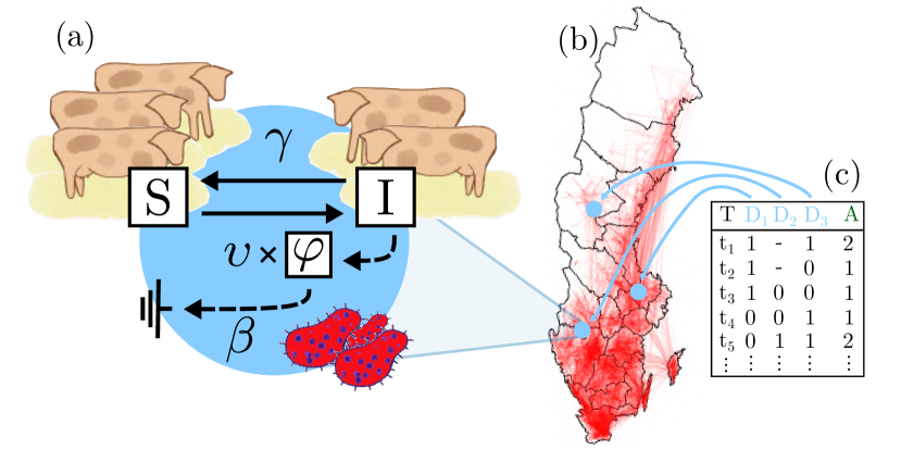
Figure 2.1: (a) The SIS_E three parameter model. Susceptible individuals $S$ turn infected at rate $\upsilon\times\varphi$. Infected individuals $I$ recover at a rate $\gamma$, and shed the pathogen to the environment adding to the infectious pressure $\varphi$, which decays at rate $\beta$. (b) National transport data form the dynamic contact network in the simulations (Sweden). (c) Time series data $D_{1}$–$D_{3}$ from single node measurements (0: not detected pathogen, 1: detected pathogen, -: missing measurement). This data is summed up and the aggregated series $A$ is passed to the Bayesian inference procedure.

Using SimInf, we connect local copies of the SIS_E model with transports of individuals over a dynamic network, thus forming our population of interest. These movements are either synthetically generated or are pre-recorded movements from an actual transport network, cf. Fig. 2.1 (b).

In summary, our epidemiological model consists of a three-parameter local SIS_E model in the form of a continuous-time Markov chain for $(S,I)$, and an ordinary differential equation for $\varphi$, connected over a network of nodes using recorded transport data at the level of batches of animals. For the specific STEC O157 application, in order to better fit data collected from a country with fairly large climate variations (Sweden), the decay parameter $\beta$ was separated into seasons $(\beta_{1,2,3,4})$ for $[$spring,summer,fall,winter$]$, with the simplifying assumption that spring and fall are equivalent $(\beta_{1}=\beta_{3})$. Temperature data from the Swedish Meteorological and Hydrological Institute was used to locally determine the duration of the seasons.

2.2 Data-driven simulations and pathogen data

While there are several options to emulate network contact details, we have utilized explicit data from the Swedish national cattle database [35, 49]. The database contains information about the individual animals in the population, including birth/death dates and movement records. The data were transformed into anonymized events for eight years of simulation over 37,220 nodes, and consist of 5,470,039 events, of which 624,493 events concern movements (Fig. 2.1 (b)) and 4,845,546 events are demographic. This type of data is commonly recorded for livestock populations in many countries [6], and is here relied upon to connect the nodes by a transport network such that the overall spread mechanism is of hybrid character [53].

Without limiting the generality of the discussion, epidemiological measurements can be regarded as a filter operating on the full epidemiological state. In our case this filter simply returns a binary answer 0 or 1 per node: infection not detected/detected, and we assume that a probabilistic model for this response is available and can be simulated in silico as a black box. The available observations of STEC O157 were collected from a subset of 126 nodes on a bi-monthly basis during the time frame 2009–2012 [48], and the results were aggregated per quarter year, see Fig. 2.1 (c). Each observation included several bacteriological samples from the farm environment resulting in a negative or positive detection per node. To truthfully mimic this in silico we rely on an urn model driven by empirically known sensitivities given an underlying node prevalence. Details concerning the pathogen detection protocol and the associated urn model are found in the Supporting Information (SI).

2.3 Approximate Bayesian Computations

The simulation-driven Bayesian setup can be summarized as follows. We regard the epidemiological model as a stochastic process $X_{t}=X_{t}(\theta)$ in continuous time, dependent upon some parameter $\theta$$=[\theta_{1},\theta_{2},\ldots]$. Data from this process is collected via some measurement filter $M(\cdot)$ operating on the state of the process at time $t_{i}$, i.e., $x_{i}=M(X(t_{i};\;\theta))$, and where the filter itself might be an additional source of noise. We assume that there is a simulator $F(\cdot)$ that simulates and measures the process such that data may be sampled in silico provided that a parameter value $\theta$ is proposed, e.g., $z\sim F(\theta)$ simulates new data $z=(z_{i})$. The likelihood $\mathbf{P}(\cdot|\theta)$ is generally computationally intractable, although in principle the problem can be formulated as a missing data problem (see e.g. [28]), these are typically very computationally intensive and difficult to implement. Instead, an alternative approach is to use simulation-driven approximate Bayesian methods which find an approximate posterior distribution.

The basic ABC rejection sampler [5] accepts proposed parameters depending on the output from a kernel function $K_{\varepsilon}(\|z-x\|)$ with distance $\varepsilon\geq 0$. A common approximation step is the use of summary statistics $s=S(z)$, effectively reducing the dimensionality of the data to compare; instead of measuring the distance between the full data, one uses the summary statistics of the data. The probability that we accept a parameter proposal from a prior $\theta^{\prime}\sim P(\theta)$ is then given by $K_{\varepsilon}(||S(z)-S(x)||)$ where $z\sim F(\theta^{\prime})$. The problem of choosing suitable summary statistics is discussed in [42, Chap. 5]. We select our summary statistics similarly to previous suggestions for systems of comparable seasonal characteristics [37, 16]. The statistics we use for our data, a time series of the number of aggregated positive samples per quarter year, are the mean prevalence per quarter and the two largest in magnitude Fourier coefficients, all in all 6 summarizing statistics coefficients.

For observed summary statistics $s_{\text{obs}}=S(x)$, the resulting ABC posterior, $\mathbf{P}_{\text{ABC}}(\theta|s_{\text{obs}})$, has the form

$$\mathbf{P}_{\text{ABC}}(\theta|s_{\text{obs}})\propto\int K_{\varepsilon}(||s-s_{\text{obs}}||)\mathbf{P}(s|\theta)P(\theta)\,ds,$$ (2.3)

where $\mathbf{P}(s|\theta)$ is the likelihood of $s=S(z)$ implied by $\mathbf{P}(z|\theta)$. If $\varepsilon\rightarrow 0$, then by the properties of the kernel function, $\lim_{\varepsilon\to 0}{\mathbf{P}_{\text{ABC}}(\theta|s_{\text{obs}})}\propto\mathbf{P}(s_{\text{obs}}|\theta)P(\theta)$. Hence the posterior is exact provided the summary statistics are sufficient, i.e., that no information is lost [42, Chap. 1]. However, this is commonly not the case and the ABC posterior is then only approximate.

2.4 Adaptive Markov chain Monte Carlo and Synthetic likelihoods

A downside of ABC rejection is its comparably low acceptance rate. Successful attempts to address this have been achieved by combining the ABC methodology with existing likelihood-based sampling methods, e.g., Metropolis-Hastings [30]. In the seminal work [52], it was observed that measured summary statistics are often asymptotically normally distributed, i.e., $s\sim\mathcal{N}(\mu,\Sigma)$ with mean $\mu$ and covariance $\Sigma$. The (limiting) likelihood of the observed summary statistic is then the probability $\mathcal{N}(s_{\text{obs}}|\mu,\Sigma)$, usually referred to as the synthetic likelihood (SL). Since $\mu$ and $\Sigma$ are not known they must be estimated, and a natural idea is to replace them by sample estimates from multiple simulations of $z$ with the same proposal $\theta^{*}$:

$$\mathbf{S} =(S_{i})=(S(z_{1}),S(z_{2}),\dots,S(z_{N})),\qquad z_{j}\sim F(\theta^{*}),$$ (2.4)

$$\hat{\mu} =\frac{1}{N}\sum_{i=1}^{N}S_{i},$$ (2.5)

$$\hat{\Sigma} =\frac{1}{N-1}\sum_{i=1}^{N}(S_{i}-\hat{\mu}){(S_{i}-\hat{\mu})}^{\top},$$ (2.6)

for which the log-SL is

$$\log\mathcal{N}(s_{\text{obs}}|\hat{\mu},\widehat{\Sigma})=-\frac{1}{2}{(s_{\text{obs}}-\hat{\mu})}^{\top}\widehat{\Sigma}^{-1}(s_{\text{obs}}-\hat{\mu})-\frac{1}{2}\log|\widehat{\Sigma}|-\frac{N\mbox{dim}(s)}{2}\log(2\pi).$$ (2.7)

Now consider the SL as $N\rightarrow\infty$. Under broad assumptions (2.5)–(2.6) will converge to $(\mu,\Sigma)$. However, the limit can be computationally impractical for models which are expensive to simulate. An approach to improve the estimate of SL is by using the bootstrap [10], and [16] recently proposed an empirical bootstrapping procedure designed specifically for SL-driven algorithms. We found that it successfully produced more robust estimates of the SL using fewer model calls. The idea is to first determine an empirical distribution $\hat{F}_{N}(\theta^{*})$ by using $N$ independent simulations as follows. We compute synthetic data $(z_{ij})$, where $i=1,\ldots,N_{\text{time}}$ runs over time as before and $j=1,\ldots,N$ runs over the number of independent trajectories used. Notably, the empirical distribution is a distribution over $\mathbf{R}^{N_{\text{time}}}$ and is constructed by assuming each trajectory to yield $N_{\text{time}}$ independent samples, one per each point in time. While this assumption is not exactly fulfilled, the measurements are well separated in time such that independence should be at least an accurate approximation.

From the empirical distributions, we next sample $R\gg N$ new such time series by iterating through the $N_{\text{time}}$ time points, independently sampling with replacement from each of the $N$ recorded simulated trajectories, and building up in this way each sampled time series. The use of the bootstrap scheme thus results in a larger dataset, effectively bootstrapping the estimate closer to the desired limit of $N\rightarrow\infty$. Practically, the sample sizes used in our experiments were $N=20$ and $R=100$.

The SL can be used in any desired likelihood-based inference method. We chose to implement the SL in an Adaptive Metropolis (AM) scheme [22]. Instead of sampling proposals from a fixed prior distribution, the AM scheme samples adaptively using a Gaussian with covariance matrix computed from the previous entries in the Markov chain [22],

$$C_{i+1}=\frac{i-1}{i}C_{i}+\frac{\xi_{d}}{i}\left(i\bar{\theta}_{i-1}\bar{\theta}^{\text{T}}_{i-1}-(i+1)\bar{\theta}_{i}\bar{\theta}^{\text{T}}_{i}+\theta_{i}\theta^{\text{T}}_{i}+\epsilon I_{d}\right),$$ (2.8)

which does not add significant computational time, since the running mean of the chain $\bar{\theta}_{i}$ can be computed recursively. In (2.8), $\xi_{d}$ is a tuning parameter for the proposal distance, as in regular Metropolis [34], and one uses a small value $\epsilon$ to prevent a possible degeneration of $C_{i}$. The adaptivity results in the loss of the Markov property between samples, however, the chain keeps the desired ergodic properties of its non-adaptive counterpart [22, 2].

We refer to the combined algorithm as Bootstrapped Synthetic Likelihood Adaptive Metropolis (SLAM) (Alg. 1).

Algorithm 1 Synthetic Likelihood Adaptive Metropolis (SLAM).

1:Summarized data $s_{\text{obs}}$ and initial guess $(\theta_{1},\mathcal{L}_{\theta})$. Adaptivity parameters $i_{0}$, $C_{0}$, $\xi_{d}$, and $\epsilon$ (see text for details).

2:for $i=2,\dots,N_{\text{sample}}$ do

3:     if $i>i_{0}$ then Compute $C_{i}$ by (2.8) else $C_{i}=C_{0}$

4:     Sample $\theta^{*}\sim\mathcal{N}(\theta_{i-1},C_{i})$

5:     Simulate $Y=\big{(}y_{1},\dots,y_{N}\big{)},y_{j}\sim F(\theta^{*})$

6:     Bootstrap $Z=\big{(}z_{1},\dots,z_{R}\big{)},z_{j}\sim\hat{F}_{N}(Y)$

7:     Estimate $(\hat{\mu}_{\theta^{*}},\widehat{\Sigma}_{\theta^{*}})$ from $S=\mathbf{S}(Z)$, with (2.5) and (2.6)

8:     Compute $\mathcal{L}_{\theta^{*}}=\mathbf{P}_{\theta^{*}}(s_{\text{obs}}|S)$ by (2.7)

9:     if $\text{Uniform}(0,1)<\min\big{(}1,\mathcal{L}_{\theta^{*}}/\mathcal{L}_{\theta}\big{)}$ then

10:         $\theta_{i}=\theta^{*}$ and $\mathcal{L}_{\theta}=\mathcal{L}_{\theta^{*}}$

11:     else

12:         $\theta_{i}=\theta_{i-1}$      

After running the adaptive Metropolis sampler for $N_{\text{train}}$ proposals using $P$ independent parallel replicas, all with independent initial starting points, the AM has explored the support of the posterior. To refine the sample resolution, we next deploy a Metropolized Independent Sampler (MIS) [23], for $N_{\text{sample}}$ proposals, again running in $P$ independent parallel replicas. These replicas all use a single static normal proposal density, namely the aggregate of the training replicas (mean of normal means and covariances after removal of a burn-in transient). The use of a MIS lowers the correlation between samples and shortens the burn-in time. Additionaly, using a prior adapted proposal distribution, the MIS sample rate is more resource efficient than the training phase. This scheme of combining AM and MIS is remindful of the block-adaptive strategy proposed in [24], however, without any further adaptation after the first block, see Alg. 3 in the SI.

2.5 Parametric bootstrap and estimator efficiency

The target of a Bayesian approach to parameterization is the parameter posterior distribution $\mathbf{P}^{*}$ and its samples $\Theta^{*}\sim\mathbf{P}^{*}$. In practice, the best one can hope for is approximate posterior samples $\tilde{\Theta}\sim\tilde{\mathbf{P}}$, obtained from a numerical model which approximates the processes underlying the data, and using some approximate posterior sampling procedure. The error in the Bayesian posterior estimator is then formally the difference $\tilde{E}:=\tilde{\Theta}-\Theta^{*}$, but without any useful dependency relation between $\mathbf{P}^{*}$ and $\tilde{\mathbf{P}}$, one in practice seeks to quantify some statistics of this error. Useful such measures are typically derived from a point estimator of $\Theta^{*}$ and we consider the minimum mean square error estimator (MMSE) for this purpose, which is just the mean of the true posterior, $\theta^{*}:=\operatorname{\mathbb{E}}[\Theta^{*}]$. The mean square error is then

$$\tilde{e}^{2} :=\operatorname{\mathbb{E}}[(\tilde{\Theta}-\theta^{*})^{2}]=\underbrace{\operatorname{\mathbb{E}}[(\tilde{\Theta}-\tilde{\theta})^{2}]}_{\text{Variance}}+\underbrace{(\tilde{\theta}-\theta^{*})^{2}}_{\text{Square bias}},$$ (2.9)

where $\tilde{\theta}:=\operatorname{\mathbb{E}}[\tilde{\Theta}]$ is the MMSE of $\tilde{\Theta}$. This decomposes the mean square error into the variance of $\tilde{\Theta}$ and the square of the bias $\tilde{b}:=\operatorname{\mathbb{E}}[\tilde{E}]=\tilde{\theta}-\theta^{*}$.

The procedure we propose for estimating the bias falls under the class of methods referred to as parametric bootstrap [10]. The general idea is to treat inference about $\mathbf{P}^{*}$ for the original data as comparable to inference of $\tilde{\mathbf{P}}$ for resampled synthetic data. We thus use the same Bayesian posterior sampling used to sample from $\tilde{\mathbf{P}}$ a second time and produce samples $\tilde{\tilde{\theta}}\sim\tilde{\tilde{\mathbf{P}}}$, that is, from the posterior given synthetic data generated from known parameters. The synthetic data may be generated by either parameters drawn from $\tilde{\mathbf{P}}$, or from an associated point estimator. We simply used the MMSE for this step and generated data using the sample mean from the posterior $\tilde{\mathbf{P}}$, that is, for $\hat{\theta}:=N_{\text{sample}}^{-1}\sum_{i}\tilde{\theta}_{i}$, where $(\tilde{\theta}_{i})$ are samples from $\tilde{\mathbf{P}}$. The error in this data-synthetic inference is $\tilde{\tilde{E}}:=\tilde{\tilde{\Theta}}-\hat{\theta}$, and hence its bias is $\tilde{\tilde{b}}:=\operatorname{\mathbb{E}}[\tilde{\tilde{E}}]$, readily estimated as a sample mean. The bootstrap estimate of the wanted bias is then simply $\tilde{b}\approx\tilde{b}_{\text{BS}}:=\tilde{\tilde{b}}$, which together with the sample variance of $(\tilde{\theta}_{i})$ yields the bootstrap estimate of the mean square error as in (2.9).

For our data we generated $M_{\text{boot}}=10$ posterior distributions $\tilde{\tilde{\mathbf{P}}}$ using independent model data realizations from the same parameter $\hat{\theta}$. Each distribution consisted of $N_{\text{sample}}=45$ samples, after removal of burn-in ($=500$) and thinning (every $100$th). Finally, the estimated bias was computed as the average bias across the $M_{\text{boot}}$ bootstrap posteriors.

3 Results

We first look into the issue of the model’s identifiability by working through a set of synthetic set-ups on smaller scale using known-truth data. The rationale here is that, if this phase does not succeed, there will be little hope in coping with more realistic situations. Results on this are reported in §3.1 where, as a side-effect, we also quantify the efficiency of the SLAM compared to the basic ABC rejection procedure. Our main results are found in §3.2 where a full national scale STEC O157 model based on first principles is parameterized from available pathogen data. Applications concerning detection and intervention scenarios are exemplified in §§3.3–3.4.

3.1 Identifiability and the efficiency of SLAM

Given real-world pathogen data and a disease spread model with an intractable likelihood, the options to rigorously analyze the parameters’ identifiability are quite limited. A practical approach is to evaluate how well a proposed inference method performs on synthetic data drawn from a known model. By testing different inference procedures on a problem with an established truth and comparing their estimation qualities, we empirically reveal both identifiability and estimator efficiency. In the Bayesian setting we may, for example, compare the error in some point estimator derived from the posterior, e.g., the average of the posterior samples (the minimum mean square error estimator). If the stability of the inference procedure remains when confronted with real data, then we may use the bootstrap procedure discussed in §2.5 to more rigorously assess the quality of the posterior.

Our full scale national model is computationally expensive, particularly so considering that parameterization requires large quantities of sample trajectories. To more effectively explore the limits of the methodology, we initially consider a synthetic set-up at a smaller scale. We define this scaled down model over 1,600 nodes, using synthetically generated movements of individuals for four years while recording the full epidemiological state every 60th day on a sample of 100 randomly chosen nodes (see the SI for details on how this was done in practice). We now ask if this synthetic data can be used to reliably infer the parameters used in the local infection model: $\upsilon$, $\beta$, and $\gamma$. We artificially construct some seasonality by using two values of $\beta$, that is, $\beta_{1}$ and $\beta_{2}$ each cover a 6-month period of the year, and we consider this modeling choice to be part of the prior information together with precise knowledge of the initial state at time $t=0$. This synthetic set-up is fast to simulate but preserves many of the main characteristics of the full national scale model.

We supply this system with parameters which, after some initial trial and error, were found to be reasonably close to the domain of relevance for the STEC O157 application later considered. Data from a single simulation was fed into an off-the-shelf ABC rejection sampler as well as into our own SLAM posterior sampler. The procedures were initially given “unfiltered” data in the form of the exact disease prevalence, i.e. the fraction of infected individuals, at the 100 selected nodes and at the sample points in time. Later, we moved on to binary filtered data obtained by subjecting the full state to a computational model of a certain pathogen detection protocol, see the discussion in §2.2 with further details in the SI (cf. also Fig. 2.1 (c)). Intuitively, one expects a hopefully acceptable loss of estimator accuracy when switching to filtered data.

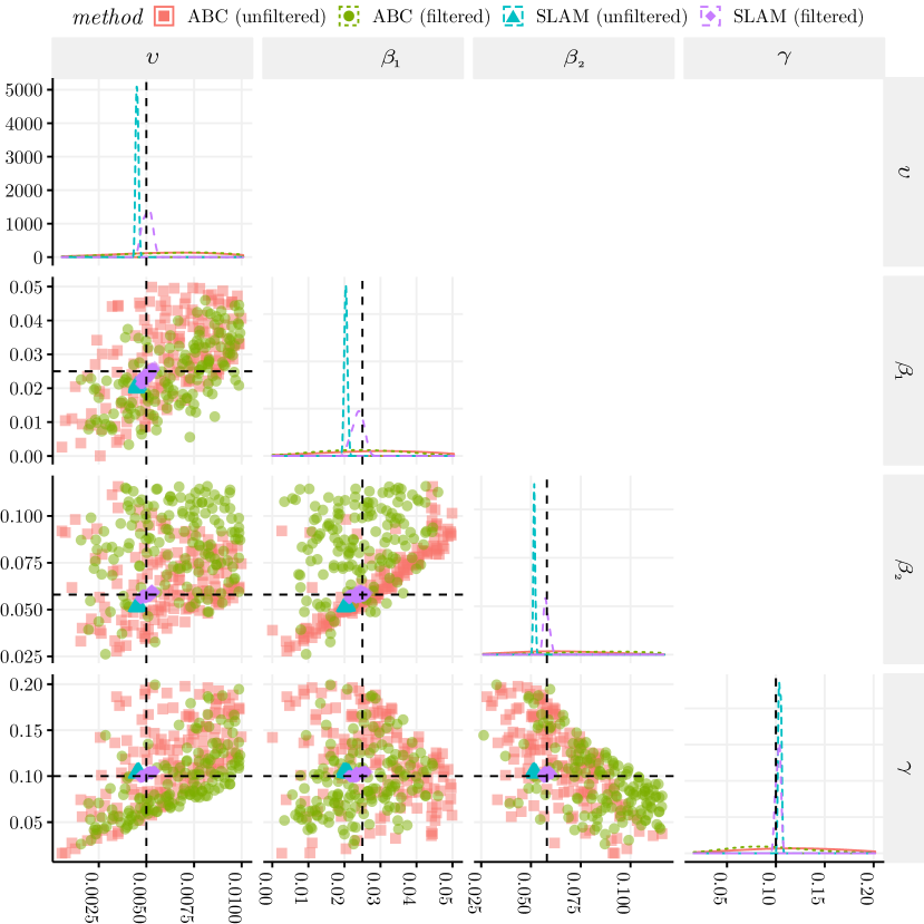
Figure 3.1: Posterior samples for the 1,600 nodes synthetic dataset (positive uniform unnormalized priors). The samples, indicated by distinct colors and shapes, are generated by either ABC rejection (on unfiltered & binary filtered data) or SLAM (on unfiltered & binary filtered data). The true parameters are indicated by the horizontal and vertical black & dashed lines. For comparable results both methods were run the same amount of wall-clock time. The plots on the diagonal are the marginal posterior distribution per parameter. The lower diagonal plots are bi-dimensional posterior samples. The axis show the parameter values, except for the top left plot’s $y$-axis which is the density.

The resulting posteriors are shown in Fig. 3.1. All samplers were successful in this synthetic setting. For SLAM, filtering the data implies a small increase in posterior width, and a minor improvement of the mean posterior bias. Although the effect in bias is a bit surprising, the difference is quite small and, moreover, a shift in bias is suitable to handle through bootstrapping estimates as is done in §3.2. The quality of the ABC sampler is somewhat more difficult to assess. Since unfiltered data is a best possible scenario, this case also defines an upper bound of the posterior quality. For the ABC sampler, the filtered state observations yield a posterior which is seemingly unaffected by the data being filtered. Since proposals are accepted under an $\varepsilon$-criterion, and since with different kinds of data, the meaning of $\varepsilon$ varies, the unfiltered and filtered versions can not be directly compared. Perhaps more interestingly, the error of the SLAM MMSE estimator is almost one order of magnitude smaller than that of the corresponding ABC-estimator (see the SI for exact errors), conditioned on using the same amount of wall-clock time. These results show that the transition from a straightforward ABC rejection sampler to a posterior obtained via a synthetic likelihood ansatz can pay off well.

3.2 National scale Bayesian inversion

As we now show, SLAM is successful in inverting a full national scale model of the spread of STEC O157 using the pathogen data from [48]. We consider anew the SIS_E model in Fig. 2.1 (a), now replicated across 37,220 actual nodes (herds) populated by about 1.6 million individual animals, and connected by the full eight year national scale animal movement dataset over Sweden (Fig. 2.1 (b)). The model parameters are $(\upsilon,\beta_{1},\beta_{2},\beta_{4},\gamma,p_{0})$, where $(\beta_{1,2,3,4})$ is the decay of infectious matter for $[$spring,summer,fall,winter$]$, and $\beta_{1}=\beta_{3}$ to simplify. As mentioned, seasons were inferred on a per-node basis using climate data from the Swedish Meteorological and Hydrological Institute. The parameter $p_{0}$ is a compact description of the system’s initial state as follows. On initialization the total number of individuals $S_{0}+I_{0}$ at each node is known from data, and we first sample $I_{0}$ to match any proposed prevalence $p_{0}$: $I_{0}/(S_{0}+I_{0})\approxeq p_{0}$. Effectively assuming equilibrium ($\varphi^{\prime}(0)\approx 0$ in (2.2)), we next set the node’s initial environmental infectious pressure to be $\varphi_{0}=\beta^{-1}I_{0}/(S_{0}+I_{0})$.

The pathogen data from [48] is understood as the result of the binary filter applied to the full state of the tested node. The measures are low-informative on the epidemiological state and distributed sparsely in both space and time: about 6–8 binary true/false samples per year, and only at 0.3% of the nodes. The computational complexity is a significant difficulty of any realistic inverse problem. For each parameter proposal, we estimate the synthetic likelihood from $N=20$ trajectories, bootstrapped to $R=100$. One trajectory results from about $10^{8}$ simulated events such that, in the end, each proposal is evaluated in about 60s over 16 compute cores ($2\times\text{Intel Xeon E5--2660}$). Similar to the inversion of the 1,600 node network in §3.1, before using any real observations, we tested the feasability using synthetic known-truth observations.

We obtain the approximate posterior parameter distribution of the STEC O157 endemics in Fig. 3.2. We next perform parametric bootstrap as discussed and improve on our confidence in the results by leveraging the stability of the inference procedure as follows. The posterior mean is used as a suitable parameter to replicate new synthetic data for, and the inference procedure is put to work again using this data. Here we apply SLAM both to the synthetic unfiltered data as well as to the filtered version. As seen in Fig. 3.2 the posterior distributions all match very closely. We quantify the accuracy of the minimum mean square error (MMSE) parameter point estimator through the MSE for the three posteriors. The bias is unknown for the most interesting case of real observations and we there have to impute the bias via the corresponding synthetic quantities, resulting in a bootstrapped/imputed estimated accuracy of the point estimator [10]. All MMSE parameter estimators were found to be within 10% accuracy and in most cases within 5% (see SI).

The posterior fit to data can be judged by comparing our estimated node prevalence of $11.2[7.9,15.5]\%$, at $95\%$ credible interval (CI) from $N=250$ posterior parameters, to the reported value $13.1\%$ [48]. We further validated our posterior by looking at two independent observational studies. We estimated the temporal population prevalence to $2.2[1.5,3.5]\%$ for (2008–09) and, respectively, to $2.2[1.5,3.3]\%$ (2011–12) ($N=250$, $95\%$ CI). These measures compare well to the studies [14, 15], where those figures are $3.3\%$ and $3.1\%$, respectively. In Fig. 3.3 the posterior simulator is also compared more directly to data.

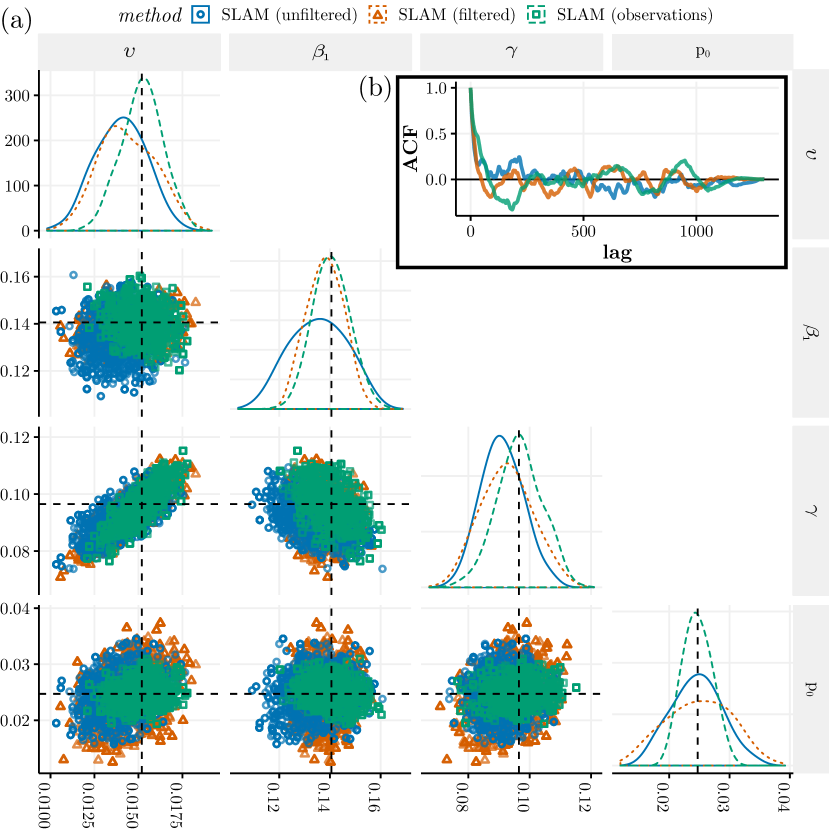
Figure 3.2: (a) Posterior parameter samples obtained from SLAM given synthetic unfiltered data, binary filtered data, and real pathogen observations (positive uniform unnormalized priors). The multivariate Gelman and Rubin’s convergence diagnostic for each method is [1.05, 1.09, 1.07]. A version of the figure including all $\beta$ dimensions is found in the SI. The horizontal and vertical black & dashed lines are the MMSE estimators from SLAM (observations): $(\upsilon,\beta_{1},\gamma,p_{0})=(0.0151,0.141,0.0965,0.0247)$. (b) The autocorrelation of the samples from one of the parallel chains of the parameter $\upsilon$.

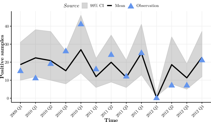
Figure 3.3: Posterior predictive check: the observations of the full system and $N=2000$ posterior sample trajectories. The blue triangles are the observations of the number of aggregated positive samples per quarter, the solid black line is the mean of the posterior samples and the shaded area is the 99% credible interval.

For the parameters, our accuracy can be summarized as an average coefficient of variation of around 7%, while previous comparable attempts obtain around 30% [17, 18, 20, 32, 8, 7], albeit in most cases for point estimators (a notable exception is [7], which also fit a stochastic national scale livestock disease model incorporating movement data within a Bayesian (ABC) framework). From our experience, the most decisive steps towards the quality of our results were (1) the good topological agreement in the prior model formulation through the combined effects of detailed network data and a local climate-dependent $\beta$, (2) the effective parameterization of the initial state through the scalar $p_{0}$, and (3), the use of empirical bootstrapping to increase the robustness in estimating the synthetic likelihood. Additionally, using adaptive Metropolis proposals increased the sampling efficiency considerably.

3.3 Detection: large nodes are nearly optimal sentinels

The number of human STEC O157 cases is less than about 10 per 100,000, but the risk for children is considerably higher than for adults. Infected individuals often develop bloody diarrhea, and about 5–10% further develop hemolytic-uremic syndrome, a severe complication that can be fatal [38]. By reviewing surveillance routines and mitigation strategies, one could reduce the prevalence of STEC O157 in reservoirs, e.g., in the cattle population, thus potentially reducing the number of human infections [3, 49, 27]. The process of selecting sentinel nodes has been actively studied [25, 3, 41], and here we propose a way by which the sensitivity of the pathogen detection procedures can be improved within our framework.

We test five different kinds of sentinel node sets, each of the same size (10 nodes), and evaluate their detection sensitivity through multiple simulations, using $N=250$ sample parameters from the previously computed parameter posterior. The first four sets are defined in terms of simple network measures, namely indegree (Indegree), outdegree (Outdegree), node population (Largest), and, for reference, a random set (Random). We design the fifth set (Observation) to be nearly optimal as follows. We first simulated independent trajectories for eight years, while recording the infectious pressure $\varphi$ during the final four years. By ranking the nodes in the system according to the environmental pathogen load $\varphi$, we obtained a shortlist of the 10 most infected nodes, and we let these serve as a close to optimal detection set of nodes.

For the evaluation of the node detectability, the system is simulated using parameters from the posterior distribution. We define the detection sensitivity for the sentinel nodes by using a simple detection probability model as follows. At node set $\mathcal{N}_{i}$ and at time $t$, compute $\mathbf{P}(\text{detect infection})=1-\prod_{i\in\mathcal{N}_{i}}(1-P_{i}(\varphi_{i}(t)))$, where $P_{i}(\cdot)$ is modeled by a sigmoid function, $P_{i}(x)=1/[1+\exp(-k(x-\varphi_{0}))]$, where $k$ is the test’s sharpness and $\varphi_{0}$ the cut-off. Although our choice of sigmoid parameters is not important for our purposes and were arbitrary, the modeling choices here can clearly be made to mimic any empirically known sensitivity.

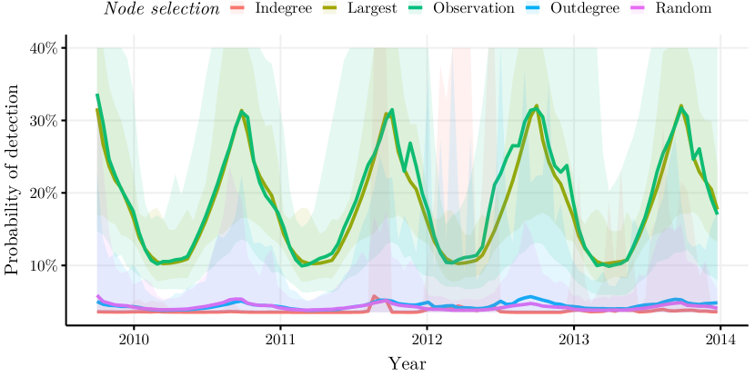
Figure 3.4: The detection probability over time for five different sets of sentinel nodes. The node sets Indegree, Largest, and Outdegree were defined from basic network statistics, and Random using uniform node sampling. The Observation set is found through pre-simulation and is nearly optimal. Each set included the 10 highest ranking nodes according to each criterion. Displayed is the mean detection probability and 95% CI. Sigmoid model parameters: $k=15$ and $\varphi_{0}=0.375$, for which $\varphi\in[0.13,0.62]$ forms a symmetric 95% CI.

The measured detection probability, displayed in Fig. 3.4, shows that the node set Largest is about as efficient as the upper limit estimate Observation. An explanation for the apparent efficiency of population size as a priority measure for detection procedures lies in the rescue effect [26], which states that, in a metapopulation with high interconnectivity, the larger nodes take the role of “rescuing” the disease from extinction; an early observation of this phenomenon was made in [19] in a study of measles. The largest nodes tend to remain continuously infected such that the infectious pressure is larger than elsewhere. This is also consistent with large groups of cattle being more likely to be STEC positive [46, 11]. The marginal performance differences between sets based on outdegree and indegree is in line with previous findings [3], that is, they do not show a significant improvement to using randomly selected nodes. Note also the clear periodic trend which could well be exploited to propose further refined detection strategies.

3.4 Intervention: best results from local actions

An important purpose with a computational epidemiological framework is to asses the effects of interventions. In [33, 39] the efficiency of mitigation strategies for epidemics were evaluated using data-driven agent-based models, and a Bayesian node-based framework was employed for the same purpose in [7]. For STEC O157, [51] proposes and assesses various interventions, although not in a probabilistic framework. We test comparable intervention proposals in our Bayesian in silico model.

We sample 250 model parameters from the posterior and simulate for four years to avoid any transient effects. Then we intervene according to three strategies as follows. The first strategy is to remove transmission by transport, i.e., if an infected animal is moved we change the status to susceptible on arrival. The second strategy is to increase the bacterial decay rate $\beta$ by 10%, and the third is to reduce the indirect transmission rate $\upsilon$ by 10%. These interventions do not invalidate the recorded transport events and therefore do not interfere with any implicit causality. After the selected intervention we record the population prevalence for five more years.

In line with the results of [51], in Fig. 3.5 we conclude that control strategies that emphasize local intervention apparently give the best results, as after three years the infection is controlled. Although the precise interpretation of the local strategies needs to be defined, the relative effects on the parameters could in principle be estimated through experiments with practical procedures including, e.g., improved on-farm biosecurity or vaccination.

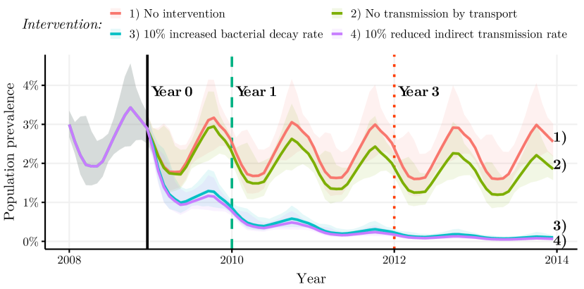
Figure 3.5: The prevalence response to intervention. Three different techniques were tested starting from the intervention point in time (solid vertical line). Displayed is the mean population prevalence and 95% CI. Measured reduction rates for each intervention protocol are reported in the SI.

4 Discussion

Epidemiological models have both qualitative and quantitative applications, and different trade-offs clearly apply depending on the purpose of the model [17, 26]. In this paper we emphasized computational models designed with the goal of assessing large-scale disease spread in a quantitative sense. This is the regime of models for which data is essential [33, 29, 47], both in driving the model, e.g., detailed network data in our case, but also in parameterizing the model using surveillance measurements. Given that pathogen surveillance data is likely to become cheaper and more accessible, e.g., with improvements in biosensors for livestock [45], data-driven models could facilitate timely and effective response to various infections.

We have demonstrated the feasibility of a Bayesian parameterization on a national scale using field data from the spread of STEC O157 in Swedish cattle. The main modeling assumptions are that network data is available and that the pathogen detection procedure can be replicated in silico. The use of a detailed transport pattern facilitates model inversion thanks to the high level of topological agreement already in the prior model formulation. For weakly informative pathogen detection protocols, we developed ideas on approaching the question of parameter identifiability via a series of controlled synthetic data experiments. Our findings here support the use of synthetic likelihoods and an adaptive Metropolis sampling over the more straightforward ABC sampler. Once parameters have been identified, parametric bootstrap enables an estimation of the confidence in the inference procedure.

With the methodology developed here a substantial improvement in the qualities of surveillance and control procedures in animal and public health is possible. We have exemplified this in the ranking of detection- and intervention procedures, where detailed credible bounds are directly available thanks to the Bayesian framework. Our work opens up the potential for better use of quantitative large-scale epidemiological models whenever sufficient data is available. With the increasing amounts of epidemiologically relevant data being collected, we conclude that there is also an important role to be played by models consistently driven by and informed from this data.

Funding

This work was financially supported by the Swedish Research Council Formas (S. Engblom, S. Widgren), by the Swedish Research Council within the UPMARC Linnaeus center of Excellence (S. Engblom, R. Eriksson), and by the Swedish strategic research program eSSENCE (S. Widgren). The simulations were performed on resources provided by the Swedish National Infrastructure for Computing (SNIC) at UPPMAX.

Supporting Information:
Bayesian epidemiological modeling
over high-resolution network data

The supporting information text consists of three parts. In the first part, we discuss the details of the available epidemiological data in the form of recorded population demographics and transport events, as well as the STEC O157 measurement procedure that was used to produce our pathogen data. The second part summarizes the ideas leading up to our specific epidemiological model and the underlying simulation engine. In the final part, we detail the Bayesian computational protocols developed and highlight some additional supporting results.

All associated data, computer codes, and experimental scripts are available online at https://github.com/robineriksson/BayesianDataDrivenModeling. The SimInf epidemiological framework is available at https://www.siminf.org.

Appendix A Epidemiological data

The data used for the full scale STEC O157 application study in the paper consists of two datasets. Firstly, anonymized network events at the level of single individuals, with 5,470,039 entries covering enter-, external transfer-, and exit events [35]. Secondly, anonymized infectious measurements of the pathogen from a longitudinal observational study [48], in which 126 cattle holdings (nodes) out of a total of 37,220 were observed for 38 months in the period 2009–2013.

Network data

We used the network data initially aggregated in [49][51], which contains processed records from the Swedish cattle database during the period in time 2005-07-01 to 2013-12-31 (102 months). The total number of cattle holdings was 37,220 which make up the epidemiological network of our simulation. The network data falls into three types of events: enter, external transfer, and exit. The enter events include births and imports from abroad. The external transfer events are movements of single individuals between the nodes of the network. The exit events imply either slaughter, euthanasia, or export of the animal to another country, i.e., the animal is removed from the observed network.

We followed an earlier prescription of handling the data in the simulator [siminf2][49]. We randomly sample the individuals from the compartments affected by the event without consideration of the infection state and after moving the animals keep the same disease state in the new holding as in the previous holding. An assumption that was consistently made was that the individuals who enter the network, i.e., are born or are imported, are in the susceptible state.

Pathogen data

As the data used for the parameterization of the national scale STEC O157 model we relied upon the longitudinal observational study in [48]. The study consisted of repeatedly collecting environmental samples from 126 Swedish cattle holdings during the period October 2009 to December 2012, with the aim of determining the presence of STEC O157 at each herd and at several points in time.

To determine the sample outcome of a simulated node, we replicated in silico the sampling protocol described in [48][49]. We proceed as follows. At the time of the measurement and at the measurement site, we randomly form testing units consisting of three individuals sampled from the pool of susceptible and infected individuals. The testing unit is classified as clean or infected with an empirically known probability [cray1995][Widgren2013], see Fig. A.1 (c). If any testing unit is found to be infected, then the whole node is classified as infected, otherwise the node is judged clean. The protocol is schematically summarized in Fig. A.1.

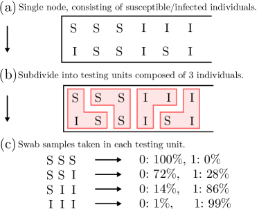
Figure A.1: (a) The population in a single node, consisting of susceptible (S) and infected (I) individuals. (b) From the node population, testing units composed of 3 individuals are formed. (c) Swab samples in each testing unit reveal infected individuals with empirically known sensitivities, 0: unit determined clean, 1: unit determined infected. The whole node is judged clean (0) provided none of the testing units are judged infected, and infected (1) otherwise.

Synthetic data

The data for the scaled down model was generated to mimic the seasonality in births, deaths and movements in the real livestock data. For the animal movements, random connections between holdings were used to generate the transport events. The synthetic data is available in the SimInf software, contains 466,692 events (exit = 182,535; enter = 182,685; external transfer = 101,472) for 1,600 holdings distributed over $4\times 365$ days.

Appendix B Epidemiological modeling

This section develops the epidemiological modeling underlying the results of the paper. The material is aimed to be as brief as possible while still being self-contained. A less concentrated exposition can be found in [12], see also [siminf2] for some more on the high-performance computing aspects. For general monographs, consult [AnderssonBrittonSIR][BrauerEpidemiology][DiekmannBrittonMathEpidemics][KeelingModeling]. The software SimInf is detailed in [SimInf_software][50] and is publicly available at www.siminf.org.

Continuous-time Markov chains

At the scale of a single node consisting of relatively few individuals, say less than a few 100s, it is generally agreed that stochastic effects can be important. A stochastic model may capture the intrinsic noise due to the parts of the dynamics not explicitly modeled, such as precise contact details of infectious agents. For a discrete state variable, namely the number of individuals in a certain epidemiological state, and in continuous time, this implies a continuous-time Markov chain as the modeling framework of choice.

Consider first the classical SIR model [Kermack1927],

$$\left.\begin{array}[]{rl}S+I&\xrightarrow{\upsilon}2I\\ I&\xrightarrow{\gamma}R\\ \end{array}\right\},$$ (B.3)

in terms of the integer state vector $X(t)=[S,I,R]=[$#Susceptible, #Infected, #Recovered$]$ individuals at time $t$. The dynamics consists of two transitions: the first increases $I$ by one and decreases $S$ analogously, and the second similarly decreases $I$ by one and increases $R$ by one. The transition rates for these transitions are understood to be the associated combinatorial product scaled with the corresponding rate parameter; this is $\upsilon SI=\upsilon X_{1}(t)X_{2}(t)$ for the first, and $\gamma I=\gamma X_{2}(t)$ for the second transition.

We may compactly write the stochastic SIR-model in the form of a mass action jump stochastic differential equation (jump SDE) as follows. Assume a probability triplet $(\Omega,\mathcal{F},\mathbf{P})$ supporting Poisson processes for the different transitions. The state vector $X(t)=X(t;\,\omega)\in\mathbf{Z}_{+}^{3}$, $\omega\in\Omega$, counts at time $t$ the number of individuals in each of the 3 compartments $S$, $I$, and $R$. Define the stoichiometric coefficients and the transition rates following the previously described logic of the SIR model,

$$\mathbb{S} =\left[\begin{array}[]{rr}-1&0\\ 1&-1\\ 0&1\end{array}\right],\quad R(x)=[\beta x_{1}x_{2},\gamma x_{3}]^{T}.$$ (B.7)

The Markovian steps are the columns of $\mathbb{S}$ and their corresponding intensities are the elements in $R$. A compact form for the resulting mass-action continuous-time Markov chain is now

$$dX(t) =\mathbb{S}\boldsymbol{\mu}(dt),$$ (B.8)

where by $\boldsymbol{\mu}(\cdot)$ we mean a state-dependent vector random counting measure of deterministic intensity $R(\cdot)$,

$$\operatorname{\mathbb{E}}[\boldsymbol{\mu}(dt)] =\operatorname{\mathbb{E}}[\boldsymbol{\mu}(x,dt)]=R(x)dt=[\upsilon x_{1}x_{2},\gamma x_{2}]^{T}dt.$$ (B.9)

Epidemiological events are thus prescribed to arrive according to competing Poisson processes of the corresponding intensities. An event $r$ at time $t$ implies that the state is to be changed according to the prescription $X(t)=X(t-)+\mathbb{S}(:,r)$.

It is convenient to capture also events scheduled ahead of the simulation with the same notation. The most important such event is the physical transport of individuals between nodes, but also demographic events can be modeled equivalently. A priori scheduled events at times $(t_{i})$ are thus associated with a sum of temporal Dirac measures,

$$\mu_{3}(dt) =\sum_{i}\delta(t_{i};\,dt),$$ (B.10)

together with an appropriate additional third column in $\mathbb{S}$.

Mixed discrete-continuous states

At a sufficiently large modeling scale there will usually be concentration type variables for which an ODE-based description is more natural. The obvious example is the concentration of bacteria in an environment for which counting is impossible. A general mixed jump SDE-ODE model ansatz is

$$\begin{array}[]{rcl}dX(t)&=&\mathbb{S}\boldsymbol{\mu}(dt)\\ Y^{\prime}(t)&=&f(X(t-),Y(t))\\ \end{array}$$ (B.13)

where $(X,Y)\in\mathbf{Z}^{M_{\mbox{{\tiny comp}}}}\times\mathbf{R}^{M_{\mbox{{\tiny conc}}}}$ and where the counting measure may now depend also on the concentration variable; $\operatorname{\mathbb{E}}[\boldsymbol{\mu}(dt)]=R(x,y)dt$.

The model favored in the paper is the SIS_E model which can be defined from two integer states $X=[S,I]$, and one concentration variable, $Y=\varphi$, the concentration of infectious substance. The SIS_E model follows from the specific choices

$$\mathbb{S} =\left[\begin{array}[]{rr}-1&1\\ 1&-1\end{array}\right],\quad R(x,y)=[\upsilon x_{1}y_{1},\gamma x_{2}]^{T},\quad f(x,y)=\alpha x_{2}(x_{1}+x_{2})^{-1}-\beta y_{1}.$$ (B.16)

The rationale here is that infected individuals are recruited from the susceptible population at a rate proportional to the concentration of infectious substance. The concentration variable in turn is increased at a rate proportional to the proportion of infected individuals, and decreased according to a decay parameter $\beta$. It is straightforward to show by non-dimensionalization that $\alpha=1$ may be selected without losing any generality [12]. The SIS_E model is summarized schematically in Fig. B.1.

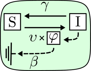
Figure B.1: The SIS_E three parameter model. Susceptible individuals S turn infected at rate $\upsilon\times\varphi$. Infected individuals I recover at a rate $\gamma$, and shed the pathogen to the environment adding to the infectious pressure $\varphi$, which in turn decays at rate $\beta$.

Dynamic networks

We shall adopt a somewhat more specific notation to capture a dynamic contact network driven by data. We assume $N_{\mbox{{\tiny nodes}}}$ nodes in total and consider the state matrix $[\mathbb{X};\;\mathbb{Y}]\in[\mathbf{Z}_{+}^{M_{\mbox{{\tiny comp}}}\times N_{\mbox{{\tiny nodes}}}};\;\mathbf{R}^{M_{\mbox{{\tiny conc}}}\times N_{\mbox{{\tiny nodes}}}}]$. The local dynamics is modeled by $N_{\mbox{{\tiny nodes}}}$ replicas of (B.13),

$$\begin{array}[]{rcl}d\mathbb{X}^{(i)}(t)&=&\mathbb{S}\boldsymbol{\mu}^{(i)}(dt)\\ \frac{d}{dt}\mathbb{Y}^{(i)}(t)&=&f(\mathbb{X}^{(i)},\mathbb{Y}^{(i)})\\ \end{array}\qquad i=1,\ldots,N_{\mbox{{\tiny nodes}}}.$$ (B.19)

Assuming a given undirected contact graph $\mathcal{G}$ each node $i$ is allowed to affect the state of the nodes in the connected components $C(i)$. Similarly, node $i$ is itself affected by all nodes $j$ such that $i\in C(j)$. The resulting network dynamics can then be written as

$$\begin{array}[]{rcl}d\mathbb{X}^{(i)}(t)&=&-\sum_{j\in C(i)}\mathbb{C}\boldsymbol{\nu}^{(i,j)}(dt)+\sum_{j;\,i\in C(j)}\mathbb{C}\boldsymbol{\nu}^{(j,i)}(dt)\\ \frac{d}{dt}\mathbb{Y}^{(i)}(t)&=&-\sum_{j\in C(i)}g(\mathbb{X}^{(i)},\mathbb{Y}^{(i)})+\sum_{j;\,i\in C(j)}g(\mathbb{X}^{(j)},\mathbb{Y}^{(j)})\end{array}$$ (B.22)

for some flow intensities $\boldsymbol{\nu}$ and $g$. Although the counting measure $\boldsymbol{\nu}^{(i,j)}$ may depend on the state of the sending node $i$, the model of the paper relies fully on externally scheduled events. Also, the specific model in the paper does not include flow of the concentration variable and hence $g\equiv 0$. Note that, in any case, mass balance is respected by this form of internodal connections.

Using superposition of the local and the global dynamics we obtain

$$\begin{array}[]{rcl}d\mathbb{X}^{(i)}(t)&=&\mathbb{S}\boldsymbol{\mu}^{(i)}(dt)-\sum_{j\in C(i)}\mathbb{C}\boldsymbol{\nu}^{(i,j)}(dt)+\sum_{j;\,i\in C(j)}\mathbb{C}\boldsymbol{\nu}^{(j,i)}(dt)\\ \frac{d}{dt}\mathbb{Y}^{(i)}(t)&=&f(\mathbb{X}^{(i)},\mathbb{Y}^{(i)})-\sum_{j\in C(i)}g(\mathbb{X}^{(i)},\mathbb{Y}^{(i)})+\sum_{j;\,i\in C(j)}g(\mathbb{X}^{(j)},\mathbb{Y}^{(j)})\end{array}$$ (B.25)

for $i=1,\ldots,N_{\mbox{{\tiny nodes}}}$. The SIS_E model employed in the paper is defined by (B.16), and with $(\mathcal{G},\mathbb{C},\boldsymbol{\nu})$ taken from actual animal transport data, and $g\equiv 0$ as mentioned. Under the mentioned non-dimensionalization the model parameters are therefore tentatively $[\upsilon,\gamma,\beta]$. Due to the fact that data is collected from a country with rather large North-South climate variations (namely Sweden), the decay $\beta$ of infectious substance is further separated into seasons $[\beta_{1},\beta_{2},\beta_{3},\beta_{4}]$ for $[$spring,summer,fall,winter$]$, and where we put $\beta_{1}=\beta_{3}$. Data from the Swedish Meteorological and Hydrological Institute (SMHI) was used to determine the duration of the seasons depending on each node’s geographical location. The seasons were defined by SMHI given the average temperature for the reference period 1961–-1990: (winter) below 0°C, (spring) between 0 and 10°C, (summer) above 10°C, and (autumn) between 0 and 10°C [SMHI].

Time discretization and simulation in parallel

In order to simulate the dynamics effectively, time has to be discretized. This is particularly reasonable in the current context since data itself is sampled at a finite resolution. Put $0=t_{0}<t_{1}<t_{2}<\cdots$ and define $\Delta t_{n}=t_{n+1}-t_{n}$. The SIS_E model in the paper is simulated by operator splitting. Specifically, we employ the three-step method (recall that $g\equiv 0$)

$$\tilde{\mathbb{X}}_{n+1}^{(i)} =\mathbb{X}_{n}^{(i)}+\int^{t_{n+1}}_{t_{n}}\mathbb{S}\boldsymbol{\mu}^{(i)}(\tilde{\mathbb{X}}^{(i)}(s),\mathbb{Y}_{n}^{(i)};\;ds),$$ (B.26)

$$\mathbb{X}_{n+1}^{(i)} =\tilde{\mathbb{X}}^{(i)}_{n+1}-\int^{t_{n+1}}_{t_{n}}\sum_{j\in C(i)}\mathbb{C}\boldsymbol{\nu}^{(i,j)}(\mathbb{X}^{(i)}(s),\mathbb{Y}_{n}^{(i)};\;ds)+\int^{t_{n+1}}_{t_{n}}\sum_{j;\,i\in C(j)}\mathbb{C}\boldsymbol{\nu}^{(j,i)}(\mathbb{X}^{(i)}(s),\mathbb{Y}_{n}^{(i)};\;ds),$$ (B.27)

$$\mathbb{Y}_{n+1}^{(i)} =\mathbb{Y}_{n}^{(i)}+f(\tilde{\mathbb{X}}_{n+1}^{(i)},\mathbb{Y}_{n}^{(i)})\,\Delta t_{n}.$$ (B.28)

The local stochastic dynamics is first simulated in time in (B.26) to produce the temporary variable $\tilde{\mathbb{X}}$. All connecting transport events are next incorporated in (B.27). Finally, in (B.28) the local dynamics for the concentration variables is computed by the standard Euler forward method in time with time-step $\Delta t_{n}$.

Appendix C Bayesian methodology

This section discusses some additional details of the Bayesian computational methodology developed in the paper.

Notation.

In the previous section we used a detailed notation for the epidemiological process defined over $N_{\mbox{{\tiny nodes}}}$ nodes. This level of detail is unnecessary here and we shall simply write $X_{t}$ for this process.

Unfiltered and binary filtered data

Recall that the epidemiological model is a stochastic process $X_{t}=X_{t}(\theta)$, with parameter $\theta$. Define the prevalence operator for a time series of state observations $(X_{i})=(X(t_{i}))$ by

$$\operatorname{Prevalence}((X_{i})) =\left(\sum_{j}I_{ij}/\sum_{j}(S_{ij}+I_{ij})\right),$$ (C.1)

that is, $\operatorname{Prevalence}(\cdot)$ computes the total prevalence in the parts of the network selected for observation and at the given points in time. The resulting time series was what was considered as “unfiltered data” in the paper, remindful of the fact that the prevalence is a deterministic function of the epidemiological state. The part of the network selected for observation was the same as the nodes where real data was available, thus facilitating a comparison.

Define further the swab operator $\operatorname{Swab}((X_{i}))$ as the outcome of the empirical stochastic swab protocol in Fig. A.1, at each point in time $t_{i}$ and at each node $j$ selected for testing. By construction, this is a stochastic function of the state and this time series was considered a realistic replication of the available data $D$, which was simply $D_{ij}=$ the outcome of the swab procedure at time $t_{i}$ and at selected node $j$.

Let finally $B(\operatorname{Swab}((X_{i})))$ and, respectively, $B(D)$ be the accumulated versions, obtained by summing up the swab results in time periods of quarter years and in $N_{\text{clusters}}$ node clusters (only 1 cluster was used in the paper). These summed-up results were referred to as the “binary filtered data” in the paper. Since the swab operator loses a fair amount of information of the epidemiological state, this case is expected to be more challenging.

To conclude, in the notation of Alg. 2 and Alg. 1 below, and as used in our tests, the required simulator $F(\cdot)$ is defined by $F(\theta)=\operatorname{Prevalence}((X_{i}))$ for unfiltered observations, and $F(\theta)=B(\operatorname{Swab}((X_{i})))$ for binary filtered data. The overall processing of data collected from the in silico disease model is schematically summarized in Fig. C.1.

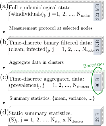
Figure C.1: Data-flow from the model’s state-space to the identifying summary statistics. (a) Full state-space of the epidemiological model. (b) After applying the pathogen detection protocol at selected nodes (see Fig. A.1) data becomes time-discrete and binary. (c) Aggregating the filtered state in clusters, and applying bootstrap resampling we obtain disease prevalence estimates at discrete points in time and in $N_{\text{clusters}}$ clusters (only 1 cluster was used in the paper). Finally, in (d) static summary statistics are extracted. The actual size of the data in each step is indicated to the right; from beginning to end data shrinks 7 orders in magnitude.

Summary statistics

We based our Bayesian procedures on six summary statistics coefficients, selected to capture seasonal dynamics as in [16][37]. The first four statistics are weighted versions of the mean of the data in each 3-month season. The fifth and sixth summary statistics are the two largest in magnitude Fourier coefficients of the data. We compute and normalize the weights $w_{i}$ for the $i$th statistics by

$$\widetilde{w}_{i} =\text{\# measurements used to compute }s_{i},$$ (C.2)

$$w_{i} =\frac{\tilde{w}_{i}}{\sum_{i}\tilde{w}_{i}}.$$ (C.3)

ABC rejection with forward simulation

In the paper, we use the uniform kernel function,

$$K_{\varepsilon}=\begin{cases}1&\text{if }||s-s_{\text{obs}}||<\varepsilon\\ 0&\text{otherwise}\end{cases},$$ (C.4)

and choose $\varepsilon$ such that only a fixed fraction of proposals are accepted. The algorithm as we deploy it is summarized in Alg. 2.

Algorithm 2 ABC rejection with forward simulation.

Summarized data $s_{\text{obs}}$

for $i=1,\dots,N_{\text{sample}}$ do

     repeat

         Propose $\theta^{*}\sim P(\theta)$

         Simulate $z\sim F(\theta^{*})$

         Summarize $s=S(z)$

     until $K_{\varepsilon}(||s-s_{\text{obs}}||)=1$

     $\theta_{i}=\theta^{*}$

Synthetic Likelihood Adaptive Metropolis with Empirical Bootstrapping

We implemented the SLAM algorithm as described in the main paper in R [RSoftware], and all the necessary data, computer codes, and experimental scripts are available online at https://github.com/robineriksson/BayesianDataDrivenModeling. An in-depth description of the Bayesian sampling procedure is found in Alg. 1.

Algorithm 3 SLAM with preprocessed Metropolized Independent Sampler.

1:Generate $\theta_{1:N_{\text{train}}}$ using SL within AM

2:Compute $\bar{C}=\text{Cov}(\theta_{1:N_{train}})$ and $\bar{\theta}=\text{Mean}(\theta_{1:N_{\text{train}}})$

3:Generate $\theta_{1:N_{\text{sample}}}$ using SL within MIS with $\bar{C}$ and $\bar{\theta}$

4:function SL($\theta$, $s_{\text{obs}}$)

5:    Simulate $Y=\big{(}y_{1},\dots,y_{N}\big{)},y_{j}\sim F(\theta)$

6:    Bootstrap $Z=\big{(}z_{1},\dots,z_{R}\big{)},z_{j}\sim\hat{F}_{N}(Y)$

7:    Estimate $(\hat{\mu}_{\theta},\widehat{\Sigma}_{\theta})$ from $S=\mathbf{S}(Z)$

8:    return $\mathcal{L}_{\theta}=\mathbf{P}_{\theta}(s_{\text{obs}}|S)$

9:function SL within AM (“SLAM)($\theta_{1}$, $\mathcal{L}_{\theta_{1}}$)

10:    for $i=2,\dots,N_{\text{train}}$ do

11:         $C_{i}:=$ if $i>i_{0}$ then $\xi\,\text{Cov}(\theta_{1},\ldots,\theta_{i-1})+\xi\epsilon I$ else $C_{0}$

12:         Sample $\theta^{*}\sim\mathcal{N}(\theta_{i-1},C_{i})$

13:         Compute $L_{\theta^{*}}=\text{SL}(\theta^{*})$

14:         $\theta_{i}=\text{accept/reject}(\theta_{i-1},\theta^{*},\mathcal{L}_{\theta},\mathcal{L}_{\theta^{*}})$     

15:    return $\theta_{1:N_{\text{\text{train}}}}$

16:function SL within MIS($\theta_{0}$, $\mathcal{L}_{\theta_{0}}$, $\bar{\theta}$, $\bar{C}$)

17:    for $i=1,\dots,N_{\text{sample}}$ do

18:         Sample $\theta^{*}\sim\mathcal{N}(\bar{\theta},\bar{C})$

19:         Compute $L_{\theta^{*}}=\text{SL}(\theta^{*})$

20:         $\theta_{i}=\text{accept/reject}(\theta_{i-1},\theta^{*},\mathcal{L}_{\theta},\mathcal{L}_{\theta^{*}})$     

21:    return $\theta_{1:N_{\text{sample}}}$

22:function accept/reject($\theta_{i-1}$, $\theta^{*}$, $\mathcal{L}_{\theta}$, $\mathcal{L}_{\theta^{*}}$)

23:    if $\mathcal{U}(0,1)<\min\big{(}1,\mathcal{L}_{\theta^{*}}/\mathcal{L}_{\theta}\big{)}$ then

24:         $\theta_{i}=\theta^{*}$ and $\mathcal{L}_{\theta}=\mathcal{L}_{\theta^{*}}$

25:    else

26:         $\theta_{i}=\theta_{i-1}$     

27:    return $\theta_{i}$, $\mathcal{L}_{\theta}$

Computational protocols and details

Throughout this work we have emphasized the need for confidence in each step forward: to achieve this we have followed the “inverse crime scheme”. Instead of starting at the final target set-up we first test the proposed method on a less complex system where a synthetic ground truth is used, and if the results are satisfactory we add complexity. This procedure is repeated until the full system is reached. On the one hand we reason at the negative side of things here: there is clearly little hope in resolving a more complex set-up without first handling an easier task. On the other hand, at each successful iteration, one gains intuition, knowledge, and confidence about the system and the method. For these reasons we first tested the proposed method on a synthetic set-up at a small-scale 1600-nodes version of the system and only then approached the full-scale version in a second step. We also tested the method initially by assuming the unfiltered state of the process could be measured, and only then moved on to considering the more realistic noisy measurement filter.

As a very first initial test, we investigated the feasibility of the parameterization by traversing a one-dimensional parameter grid on the small-scale 1600-nodes four-parameter model. We considered synthetic data from a known truth, and we fixed all parameters except for one. For this parameter we considered the domain $\text{true value}\pm 20\%$ and estimated the synthetic likelihood (SL) for the synthetic data, using multiple independent evaluations for each point ($N=20$). The purpose is to observe the definiteness in any maxima of the SL for this parameter dimension alone. We did this test for all parameter dimensions resulting in Fig. C.2. We found that $-\log\text{SL}$ is locally convex in the (one-dimensional) vicinity of every parameter, and the maxima are all apparently well-defined.

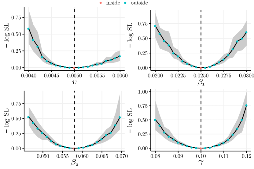
Figure C.2: The response in $-\log\text{SL}$ when diverging from the true parameter values (dashed line) and with the other parameters held fixed at their true values, $(\upsilon,\beta_{1},\beta_{2},\gamma)=(0.005,0.025,0.058,0.1)$. The SL was computed multiple $N=20$ times, and the shaded gray area represents the 95% CI. The red dots are either the minimum, or their CI overlaps with the minimum. The mean coefficient of variation for the corresponding marginal distribution was $0.2\%$.

Next we moved on to considering all parameters at once, but still for the smaller synthetic model. The inference methods tested here were ABC rejection and SLAM, first using the unfiltered- and next the binary filtered data. When comparing the two methods for the same type of data, they were run for the same amount of time. For ABC, all proposals were stored and afterwards we chose $\varepsilon$ in such a way that the same amount of samples were selected as was produced by SLAM. The results of the latter turned out to be considerably better in our tests.

Finally we considered the full national scale model. In the parameterization from actual measurements, we initialized the adaptive MCMC chain with the point estimates suggested in [51]. Because of the computationally costly character of the problem, we connected $P=10$ parallel chains on a cluster consisting of Intel Xeon E5–2660 processors. We got $10\times\numprint{1500}$ long chains from which we removed the first 500 elements as burn-in, and considered these samples as the training set $\theta_{1:N_{\text{train}}}$. The training set was then used in the MIS procedure, which resulted in $10\times\numprint{130}$ long chains, after the removal of burn-in ($100$ per chain) and thinning ($10$).

For the AM specific parameters we used $\xi_{d}=10^{-3}$, $\epsilon_{d}=10^{-5}$, $i_{0}=1$, $C_{0}=10^{-9}I_{d}$, where $i_{0}$ is the number of Metropolis iterations for which $C_{0}$ is used as the covariance matrix in the proposals (cf. Alg. 1).

Results

The errors computed and referred to in the paper are detailed in Tab. C.1 and Tab. C.2. To be able to easily compare numbers we report normalized root-mean-square errors $\text{NRMSE}:=\sqrt{\text{MSE}}/|\text{parameter value}|$.

Marginal distributions are shown in Fig. C.3, which differs from the one in the paper as it contains all the estimated parameters.

Table C.1: Errors of the ABC- and the SLAM-estimators for the synthetic small-scale problem. Normalized root-mean-square errors (NRMSE) of the minimum mean square error (MMSE) parameter estimators.

	ABC (Unfilt)	ABC (Filt)	SLAM (Unfilt)	SLAM (Filt)
$\upsilon$	$0.42$	$0.42$	$0.11$	$0.042$
$\beta_{1}$	$0.45$	$0.41$	$0.23$	$0.078$
$\beta_{2}$	$0.31$	$0.40$	$0.12$	$0.021$
$\gamma$	$0.42$	$0.39$	$0.04$	$0.031$

Table C.2: Errors of SLAM for the full problem. NRMSE with imputed bias determined from 140 accepted posterior samples. See also Fig. C.3.

Param	SLAM (Unfilt)	SLAM (Filt)	SLAM (Obs) [variance]	SLAM (Obs) [NMRSE]
$\upsilon$	$0.11$	$0.12$	$1.24\cdot 10^{-6}$	$0.08$
$\beta_{1}[=\beta_{3}]$	$0.05$	$0.09$	$4.87\cdot 10^{-5}$	$0.05$
$\beta_{2}$	$0.09$	$0.12$	$1.11\cdot 10^{-4}$	$0.09$
$\beta_{4}$	$0.10$	$0.11$	$1.37\cdot 10^{-4}$	$0.08$
$\gamma$	$0.09$	$0.08$	$5.00\cdot 10^{-5}$	$0.08$
$p_{0}$	$0.22$	$0.17$	$5.49\cdot 10^{-6}$	$0.11$

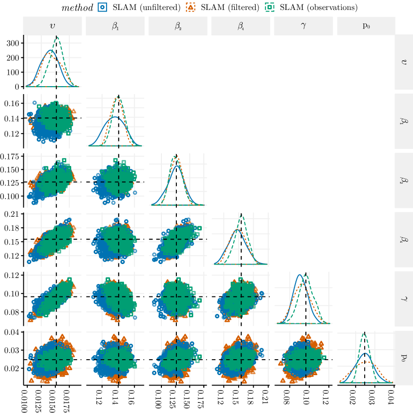
Figure C.3: Posterior samples obtained by using SLAM on unfiltered-, binary filtered state, and real observations on the full data-driven simulation over 37,220 nodes. The samples were obtained from 14,000 accepted Metropolis steps, removing 1,000 transient steps and thinning by 10. The values of the MMSE estimators thus obtained are for the case of real observations $(\upsilon,\beta_{1}[=\beta_{3}],\beta_{2},\beta_{4},\gamma,p_{0})=(0.0151,0.141,0.126,0.156,0.0965,0.0247)$.

Table C.3: Gelman-Rubin diagnostic on each parameter in the Markov chains generated from using SLAM on unfiltered-, binary filtered state, and real observations on the full data-driven simulation over 37,220 nodes

Param	SLAM (Unfilt)	SLAM (Filt)	SLAM (Obs)
$\upsilon$	$1.032$	$1.025$	$1.050$
$\beta_{1}[=\beta_{3}]$	$1.024$	$1.008$	$1.044$
$\beta_{2}$	$1.020$	$1.060$	$1.022$
$\beta_{4}$	$1.031$	$1.061$	$1.017$
$\gamma$	$1.030$	$1.017$	$1.063$
$p_{0}$	$1.036$	$1.031$	$1.038$

Intervention evaluation

In the paper, we evaluated three proposed intervention techniques. Besides the graphical investigation in the main paper we also quantified the reduction factor of the interventions, see Tab. C.4. In the table, the three interventions are measured at two points in time, and are evaluated against the case with no intervention. The quantities in the table are means with 95% CI. From these we can cannot separate intervention #3 and #4 from each other as their intervals overlap. However, they are both significantly better than intervention #2.

Table C.4: Reduction factors (mean and 95% CI) for the different intervention strategies.

Intervention strategy	Year 1	Year 3
2) No transmission via transport	$0.90\,[0.87,0.93]$	$0.79\,[0.74,0.83]$
3) 10% increased decay $\beta$	$0.33\,[0.30,0.36]$	$0.089\,[0.072,0.11]$
4) 10% reduced uptake $\upsilon$	$0.30\,[0.26,0.32]$	$0.068\,[0.053,0.089]$

References

- Anderson and May [1981] R. M. Anderson and R. M. May. The population dynamics of microparasites and their invertebrate hosts. Philosophical Transactions of the Royal Society of London. B, Biological Sciences, 291(1054):451–524, 1981. doi: 10.1098/rstb.1981.0005.
- Andrieu and Moulines [2006] C. Andrieu and É. Moulines. On the ergodicity properties of some adaptive MCMC algorithms. Ann. Appl. Probab., 16(3):1462–1505, 2006.
- Bajardi et al. [2012] P. Bajardi, A. Barrat, L. Savini, and V. Colizza. Optimizing surveillance for livestock disease spreading through animal movements. J. R. Soc. Interface, 9(76):2814–2825, 2012.
- Balcan et al. [2009] D. Balcan, V. Colizza, B. Gonçalves, H. Hu, J. J. Ramasco, and A. Vespignani. Multiscale mobility networks and the spatial spreading of infectious diseases. Proc. Natl. Acad. Sci. USA, 106(51):21484–21489, 2009.
- Beaumont et al. [2002] M. A. Beaumont, W. Zhang, and D. J. Balding. Approximate Bayesian computation in population genetics. Genetics, 162(4):2025–2035, 2002.
- Brooks-Pollock et al. [2014a] E. Brooks-Pollock, M. de Jong, M. Keeling, D. Klinkenberg, and J. Wood. Eight challenges in modelling infectious livestock diseases. Epidemics, 10:1–5, 2014a. doi: 10.1016/j.epidem.2014.08.005.
- Brooks-Pollock et al. [2014b] E. Brooks-Pollock, G. O. Roberts, and M. J. Keeling. A dynamic model of bovine tuberculosis spread and control in Great Britain. Nature, 511:228, 2014b.
- Brouwer et al. [2018] A. F. Brouwer, J. N. Eisenberg, C. D. Pomeroy, L. M. Shulman, M. Hindiyeh, Y. Manor, I. Grotto, J. S. Koopman, and M. C. Eisenberg. Epidemiology of the silent polio outbreak in Rahat, Israel, based on modeling of environmental surveillance data. Proc. Natl. Acad. Sci. USA, 115(45):E10625–E10633, 2018.
- Degli Atti et al. [2008] M. L. C. Degli Atti, S. Merler, C. Rizzo, M. Ajelli, M. Massari, P. Manfredi, C. Furlanello, G. S. Tomba, and M. Iannelli. Mitigation measures for pandemic influenza in Italy: an individual based model considering different scenarios. PLoS ONE, 3(3):e1790, 2008.
- Efron [1979] B. Efron. Bootstrap Methods: Another Look at the Jackknife. Ann. Statist., 7, 1979.
- Ellis-Iversen et al. [2007] J. Ellis-Iversen, R. P. Smith, L. C. Snow, E. Watson, M. F. Millar, G. C. Pritchard, A. R. Sayers, A. J. Cook, S. J. Evans, and G. A. Paiba. Identification of management risk factors for VTEC O157 in young-stock in england and wales. Preventive veterinary medicine, 82(1-2):29–41, 2007.
- Engblom and Widgren [2017] S. Engblom and S. Widgren. Data-driven computational disease spread modeling: from measurement to parametrization and control. In C. R. Rao, A. S. Rao, and S. Payne, editors, Disease Modeling and Public Health: Part A, volume 36 of Handbook of Statistics, chapter 11, pages 305–328. Elsevier, Amsterdam, 2017. doi: 10.1016/bs.host.2017.05.005.
- Eubank et al. [2004] S. Eubank, H. Guclu, V. A. Kumar, M. V. Marathe, A. Srinivasan, Z. Toroczkai, and N. Wang. Modelling disease outbreaks in realistic urban social networks. Nature, 429(6988):180, 2004.
- European Food Safety Authority and European Centre for Disease Prevention and Control [2012] European Food Safety Authority and European Centre for Disease Prevention and Control. The European union summary report on trends and sources of zoonoses, zoonotic agents and food-borne outbreaks in 2010. EFSA Journal, 10(3):2597, 2012. doi: 10.2903/j.efsa.2012.2597.
- European Food Safety Authority and European Centre for Disease Prevention and Control [2014] European Food Safety Authority and European Centre for Disease Prevention and Control. The European union summary report on trends and sources of zoonoses, zoonotic agents and food-borne outbreaks in 2012. EFSA Journal, 12(2):3547, 2014. doi: 10.2903/j.efsa.2014.3547.
- Everitt [2018] R. G. Everitt. Bootstrapped synthetic likelihood. arXiv:1711.05825v2, 2018. Preprint, posted 17 Jan 2018.
- Ferguson et al. [2003] N. M. Ferguson, M. J. Keeling, W. J. Edmunds, R. Gani, B. T. Grenfell, R. M. Anderson, and S. Leach. Planning for smallpox outbreaks. Nature, 425(6959):681, 2003.
- Ferguson et al. [2005] N. M. Ferguson, D. A. Cummings, S. Cauchemez, C. Fraser, S. Riley, A. Meeyai, S. Iamsirithaworn, and D. S. Burke. Strategies for containing an emerging influenza pandemic in southeast Asia. Nature, 437(7056):209, 2005.
- Finkenstädt et al. [2002] B. F. Finkenstädt, O. N. Bjørnstad, and B. T. Grenfell. A stochastic model for extinction and recurrence of epidemics: estimation and inference for measles outbreaks. Biostatistics, 3(4):493–510, 2002.
- Fournié et al. [2018] G. Fournié, A. Waret-Szkuta, A. Camacho, L. M. Yigezu, D. U. Pfeiffer, and F. Roger. A dynamic model of transmission and elimination of peste des petits ruminants in Ethiopia. Proc. Natl. Acad. Sci. USA, 115(33):8454–8459, 2018.
- Germann et al. [2006] T. C. Germann, K. Kadau, I. M. Longini, and C. A. Macken. Mitigation strategies for pandemic influenza in the United States. Proc. Natl. Acad. Sci. USA, 103(15):5935–5940, 2006.
- Haario et al. [2001] H. Haario, E. Saksman, and J. Tamminen. An adaptive Metropolis algorithm. Bernoulli, 7(2):223–242, 2001.
- Hastings [1970] W. K. Hastings. Monte Carlo sampling methods using Markov chains and their applications. Biometrika, 57:97–109, 1970.
- Jacob et al. [2011] P. Jacob, C. P. Robert, and M. H. Smith. Using parallel computation to improve independent Metropolis–Hastings based estimation. Journal of Computational and Graphical Statistics, 20(3):616–635, 2011.
- Keeling and Eames [2005] M. J. Keeling and K. T. Eames. Networks and epidemic models. Journal of the Royal Society Interface, 2(4):295–307, 2005.
- Keeling and Rohani [2008] M. J. Keeling and P. Rohani. Modeling infectious diseases in humans and animals. Princeton University Press, 2008.
- Keeling et al. [2017] M. J. Keeling, S. Datta, D. N. Franklin, I. Flatman, A. Wattam, M. Brown, and G. E. Budge. Efficient use of sentinel sites: detection of invasive honeybee pests and diseases in the UK. J. R. Soc. Interface, 14(129), 2017.
- Lau et al. [2017] M. S. Lau, G. J. Gibson, H. Adrakey, A. McClelland, S. Riley, J. Zelner, G. Streftaris, S. Funk, J. Metcalf, B. D. Dalziel, et al. A mechanistic spatio-temporal framework for modelling individual-to-individual transmission—With an application to the 2014-2015 west africa ebola outbreak. PLoS Comput Biol, 13(10):e1005798, 2017.
- Liu et al. [2018] Q.-H. Liu, M. Ajelli, A. Aleta, S. Merler, Y. Moreno, and A. Vespignani. Measurability of the epidemic reproduction number in data-driven contact networks. Proc. Natl. Acad. Sci. USA, 115(50):12680–12685, 2018.
- Marjoram et al. [2003] P. Marjoram, J. Molitor, V. Plagnol, and S. Tavaré. Markov chain Monte Carlo without likelihoods. Proc. Natl. Acad. Sci. USA, 100(26):15324–15328, 2003.
- McKinley et al. [2018] T. J. McKinley, I. Vernon, I. Andrianakis, N. McCreesh, J. E. Oakley, R. N. Nsubuga, M. Goldstein, and R. G. White. Approximate Bayesian Computation and simulation-based inference for complex stochastic epidemic models. Statist. Sci., 33(1):4–18, 2018.
- Merler et al. [2011] S. Merler, M. Ajelli, A. Pugliese, and N. M. Ferguson. Determinants of the spatiotemporal dynamics of the 2009 H1N1 pandemic in Europe: implications for real-time modelling. PLoS Comput. Biol., 7(9):e1002205, 2011.
- Merler et al. [2015] S. Merler, M. Ajelli, L. Fumanelli, M. F. Gomes, A. P. y Piontti, L. Rossi, D. L. Chao, I. M. Longini Jr, M. E. Halloran, and A. Vespignani. Spatiotemporal spread of the 2014 outbreak of Ebola virus disease in Liberia and the effectiveness of non-pharmaceutical interventions: a computational modelling analysis. The Lancet Infect. Diseases, 15(2):204–211, 2015.
- Metropolis et al. [1953] N. Metropolis, A. W. Rosenbluth, M. N. Rosenbluth, A. H. Teller, and E. Teller. Equation of state calculations by fast computing machines. J. Chem. Phys., 21(6):1087–1092, 1953.
- Nöremark et al. [2011] M. Nöremark et al. Network analysis of cattle and pig movements in Sweden: measures relevant for disease control and risk based surveillance. Prev. Veterinary Med., 99(2):78–90, 2011.
- Obadia et al. [2015] T. Obadia, R. Silhol, L. Opatowski, L. Temime, J. Legrand, A. C. Thiébaut, J.-L. Herrmann, E. Fleury, D. Guillemot, P.-Y. Boelle, et al. Detailed contact data and the dissemination of Staphylococcus aureus in hospitals. PLoS Comput. Biol., 11(3):e1004170, 2015.
- Papamakarios and Murray [2016] G. Papamakarios and I. Murray. Fast -free inference of simulation models with Bayesian conditional density estimation. In Adv. Neur. Inf. Proc. Syst., pages 1028–1036, 2016.
- Parry and Palmer [2000] S. Parry and S. Palmer. The public health significance of VTEC O157. J. Appl. Microbiol., 88(S1):1S–9S, 2000.
- Peak et al. [2017] C. M. Peak, L. M. Childs, Y. H. Grad, and C. O. Buckee. Comparing nonpharmaceutical interventions for containing emerging epidemics. Proc. Natl. Acad. Sci. USA, 114(15):4023–4028, 2017.
- Salathé et al. [2010] M. Salathé, M. Kazandjieva, J. W. Lee, P. Levis, M. W. Feldman, and J. H. Jones. A high-resolution human contact network for infectious disease transmission. Proc. Natl. Acad. Sci. USA, 107(51):22020–22025, 2010.
- Schärrer et al. [2015] S. Schärrer, S. Widgren, H. Schwermer, A. Lindberg, B. Vidondo, J. Zinsstag, and M. Reist. Evaluation of farm-level parameters derived from animal movements for use in risk-based surveillance programmes of cattle in Switzerland. BMC veterinary research, 11(1):149, 2015.
- Sisson et al. [2018] S. A. Sisson, Y. Fan, and M. Beaumont. Handbook of Approximate Bayesian Computation. Chapman and Hall/CRC, 2018.
- Stehlé et al. [2011] J. Stehlé, N. Voirin, A. Barrat, C. Cattuto, V. Colizza, L. Isella, C. Régis, J.-F. Pinton, N. Khanafer, W. Van den Broeck, et al. Simulation of an SEIR infectious disease model on the dynamic contact network of conference attendees. BMC Medicine, 9(1):87, 2011.
- Toth et al. [2015] D. J. Toth, M. Leecaster, W. B. Pettey, A. V. Gundlapalli, H. Gao, J. J. Rainey, A. Uzicanin, and M. H. Samore. The role of heterogeneity in contact timing and duration in network models of influenza spread in schools. J. R. Soc. Interface, 12(108):20150279, 2015.
- Vidic et al. [2017] J. Vidic, M. Manzano, C.-M. Chang, and N. Jaffrezic-Renault. Advanced biosensors for detection of pathogens related to livestock and poultry. Veterinary Res., 48(1):11, 2017.
- Vidovic and Korber [2006] S. Vidovic and D. R. Korber. Prevalence of escherichia coli o157 in saskatchewan cattle: characterization of isolates by using random amplified polymorphic dna pcr, antibiotic resistance profiles, and pathogenicity determinants. Appl. Environ. Microbiol., 72(6):4347–4355, 2006.
- Walters et al. [2018] C. E. Walters, M. M. Meslé, and I. M. Hall. Modelling the global spread of diseases: A review of current practice and capability. Epidemics, 25:1–8, 2018.
- Widgren et al. [2015] S. Widgren, R. Söderlund, E. Eriksson, C. Fasth, A. Aspan, U. Emanuelson, S. Alenius, and A. Lindberg. Longitudinal observational study over 38 months of verotoxigenic E. coli O157:H7 status in 126 cattle herds. Prev. Veterinary Med., 121(3-4):343–352, 2015.
- Widgren et al. [2016] S. Widgren, S. Engblom, P. Bauer, J. Frössling, U. Emanuelson, and A. Lindberg. Data-driven network modelling of disease transmission using complete population movement data: spread of VTEC O157 in Swedish cattle. Veterinary Res., 47(1):81, 2016. doi: 10.1186/s13567-016-0366-5.
- Widgren et al. [2019] S. Widgren, P. Bauer, R. Eriksson, and S. Engblom. SimInf: An R package for data-driven stochastic disease spread simulations. J. Stat. Softw., 91(12):1–42, 2019.
- Widgren et al. [2018] S. Widgren et al. Spatio-temporal modelling of verotoxigenic E. coli O157 in cattle in Sweden: Exploring options for control. Veterinary Res., 49(78), 2018. doi: 10.1186/s13567-018-0574-2.
- Wood [2010] S. N. Wood. Statistical inference for noisy nonlinear ecological dynamic systems. Nature, 466(7310):1102–1104, 2010.
- Zhang et al. [2015] C. Zhang, S. Zhou, J. C. Miller, I. J. Cox, and B. M. Chain. Optimizing hybrid spreading in metapopulations. Scientific Rep., 5:9924, 2015.
- Zhang et al. [2017] Q. Zhang, K. Sun, M. Chinazzi, A. P. y Piontti, N. E. Dean, D. P. Rojas, S. Merler, D. Mistry, P. Poletti, L. Rossi, et al. Spread of Zika virus in the Americas. Proc. Natl. Acad. Sci. USA, 114(22):E4334–E4343, 2017.

References

- Andersson and Britton [2000] H. Andersson and T. Britton. Stochastic Epidemic Models and Their Statistical Analysis, volume 151 of Lecture Notes in Statistics. Springer, New York, 2000.
- Anonymous [2016] Anonymous. Maps with the average date for the beginning of each season (spring, summer, fall, winter) for the reference period 1961–1990. The Swedish Meteorological and Hydrological Institute (SMHI), Norrköping, Sweden. http://opendata-catalog.smhi.se/, 2016. Accessed: 2016-08-25.
- Bauer et al. [2016] P. Bauer, S. Engblom, and S. Widgren. Fast event-based epidemiological simulations on national scales. Int. J. High Perf. Comput. Appl., 30(4):438–453, 2016. doi: 10.1177/1094342016635723.
- Brauer and Castillo-Chavez [2012] F. Brauer and C. Castillo-Chavez. Mathematical Models in Population Biology and Epidemiology, volume 40 of Texts in Applied Mathematics. Springer-Verlag, New York, second edition, 2012.
- Cray and Moon [1995] W. C. Cray and H. W. Moon. Experimental infection of calves and adult cattle with escherichia coli O157:H7. Appl. Environ. Microbiol., 61(4):1586–1590, 1995.
- Diekmann O. and Britton [2012] J. Diekmann O., Heesterbeek and T. Britton. Mathematical tools for understanding infectious disease dynamics. Princeton Series in Theoretical and COmput. BIol. Princeton University Press, New Jersey, first edition, 2012.
- Engblom and Widgren [2017] S. Engblom and S. Widgren. Data-driven computational disease spread modeling: from measurement to parametrization and control. In C. R. Rao, A. S. Rao, and S. Payne, editors, Disease Modeling and Public Health: Part A, volume 36 of Handbook of Statistics, chapter 11, pages 305–328. Elsevier, Amsterdam, 2017. doi: 10.1016/bs.host.2017.05.005.
- Everitt [2018] R. G. Everitt. Bootstrapped synthetic likelihood. arXiv:1711.05825v2, 2018. Preprint, posted 17 Jan 2018.
- Keeling and Rohani [2007] M. J. Keeling and P. Rohani. Modeling Infectious Diseases in Humans and Animals. Princeton University Press, New Jersey, first edition, 2007.
- Kermack and McKendrick [1927] W. O. Kermack and A. G. McKendrick. A contribution to the mathematical theory of epidemics. Proc. R. Soc. Lond. Ser. A Math. Phys. Eng. Sci., 115:700–721, 1927.
- Nöremark et al. [2011] M. Nöremark et al. Network analysis of cattle and pig movements in Sweden: measures relevant for disease control and risk based surveillance. Prev. Veterinary Med., 99(2):78–90, 2011.
- Papamakarios and Murray [2016] G. Papamakarios and I. Murray. Fast -free inference of simulation models with Bayesian conditional density estimation. In Adv. Neur. Inf. Proc. Syst., pages 1028–1036, 2016.
- R Core Team [2017] R Core Team. R: A Language and Environment for Statistical Computing. R Foundation for Statistical Computing, Vienna, Austria, 2017. Available at https://www.R-project.org.
- Widgren et al. [2013] S. Widgren, E. Eriksson, A. Aspan, U. Emanuelson, S. Alenius, and A. Lindberg. Environmental sampling for evaluating verotoxigenic Escherichia coli O157:H7 status in dairy cattle herds. J. Veterinary Diagnostic Invest., 25(2):189–198, 2013. doi: 10.1177/1040638712474814.
- Widgren et al. [2015] S. Widgren, R. Söderlund, E. Eriksson, C. Fasth, A. Aspan, U. Emanuelson, S. Alenius, and A. Lindberg. Longitudinal observational study over 38 months of verotoxigenic E. coli O157:H7 status in 126 cattle herds. Prev. Veterinary Med., 121(3-4):343–352, 2015.
- Widgren et al. [2016] S. Widgren, S. Engblom, P. Bauer, J. Frössling, U. Emanuelson, and A. Lindberg. Data-driven network modelling of disease transmission using complete population movement data: spread of VTEC O157 in Swedish cattle. Veterinary Res., 47(1):81, 2016. doi: 10.1186/s13567-016-0366-5.
- Widgren et al. [2016–2018] S. Widgren, P. Bauer, R. Eriksson, and S. Engblom. SimInf: A framework for stochastic disease spread simulations, 2016–2018. Available at www.siminf.org.
- Widgren et al. [2019] S. Widgren, P. Bauer, R. Eriksson, and S. Engblom. SimInf: An R package for data-driven stochastic disease spread simulations. J. Stat. Softw., 91(12):1–42, 2019.
- Widgren et al. [2018] S. Widgren et al. Spatio-temporal modelling of verotoxigenic E. coli O157 in cattle in Sweden: Exploring options for control. Veterinary Res., 49(78), 2018. doi: 10.1186/s13567-018-0574-2.