Abstract

In this paper, we use corrected $f(R)$ gravitational model which is polynomial function with a logarithmic term. In that case, we employ the slow-roll condition and obtain the number of cosmological parameter. This help us to verify the swampland conjectures which is guarantee the validation of low - energy quantum field theory. The obtained results shown that the corresponding model is consistent with the swampland conjectures. Also the upper and lower limit of the parameter $n$ are 0.15 and 0.0033. Finally, by using scalar spectrum index $n_{s}$ and tensor to scalar ratio $r$ relations and compared with Planck 2018 empirical data, we obtain the coefficients $\alpha$,$\beta$ and $\gamma$. Also, the corresponding results are creaked by several figures, literature and also plank 2018 data.
Keywords: Landscape, Samwpland condition, WGC, Logarithmic correction, Slow-roll

1 Introduction

As we know weak gravity conjecture (WGC) is a strong conjecture on gravitational coupling theories which shows that gravity is the weakest force in any theory consistent with quantum gravity[1, 2, 3]. There are some evidence for weak gravity conjecture which including holography, cosmic censorship, entropy, unitary and causality. In order to study swampland and landscape, for the simplicity we have distinguish between general quantum gravity with string theory[6, 7, 5, 4]. If we want to understand the abstract concept of the swampland, we have to understand how to distinguish between low energy effective field theories that are in the landscape from those in the swampland. The most important things here is WGC, because it provides a very powerful tool for distinguishing between landscape and swampland[4, 1, 5, 6]. We note here a set of consistent low energy effective field theories, which is compatible to string theory is called a landscape[8, 10, 11, 9]. We mention that also, at the low energies landscape is surrounded by wider space called swampland, which is consistent with quantum gravity. So, for more reviews about swampland, one can see Ref.s [4, 1, 8]. But, at high energies the whole space is landscape, which is consistent with quantum gravity. Generally, one can say that there are different conditions for the verifying that a low energy theory is swampland or landscape[12, 13]. One of the conditions that has been studied in recent years for the specifying about swampland is [14, 15]

$$\frac{|\Delta\phi|}{M_{pl}}\leq\Delta\sim 1$$ (1)

and

$$M_{pl}\frac{|V^{\prime}(\phi)|}{V}\geq c\sim 1$$ (2)

where $M_{pl}$ is Planck mass, we assume approximately equal one, $c$ and $\Delta$ are positive constants as order of unity [16, 10, 17, 18]. $V(\phi)$ is also the potential which is coming normalized canonical field $\phi$. The criteria of swampland have been examined in various gravitational theories, which can be found in the Ref.s.[19, 21, 20].

The first condition of above mentioned equation actually satisfies the single field inflation, but the second condition creates some problems for the single field system. Recently, new swampland conjecture models have been proposed[10, 22, 23], this new models introduce a scalar field potential associated with a self-consistent $UV$ compleat which must be satisfied by following two conditions,

$$8(M_{pl}\frac{|V^{\prime}|}{V})\geq c$$ (3)

and

$$(M_{pl}^{2}\frac{|V^{\prime\prime}|}{V})\leq-c^{\prime}$$ (4)

where $c$ and $c^{\prime}$ are unit order and constants . As you know, one of the dark energy models based on modified gravity is actually called $f(R)$ gravity . $f$ is a function of scalar Ricci, and in general we have $f=F+R$[24, 26, 25]. Such modified gravity will be suitable candidate for describing dark energy and cosmic acceleration. So, in this paper we examine the applications of WGC constraint on a deformed Starobinsky gravity[27, 28]. The purpose of this paper, we employ one part of WGC model as swampland condition. In that case, we take advantage from $f(R)$ modified gravity and examine the inflation theory. Here one can say that, the obtained results from swampland condition can be compared by experimental data. Also, we note here that several researchers worked with some simple form of $f(R)$, which are given by [30, 29, 32, 31]. But, we take another $f(R)$ which is including both polynomial and a logarithmic form. In that case, we apply the corresponding WGC condition and verify some suitable parameters in $f(R)$ gravity. All above information about the swampland condition on the cosmological model give us motivation to organized the paper as follows. In section 2, we introduce the function$f(R)$ and consider our corresponding model. In section 3, by using the above-mentioned actions, we calculate scalar field and canonical normalize potential . In section 4, also by using scalar field and canonical normalize potential we obtain the slow- roll parameters. Also, here we investigate the swampland condition. In section 5, we calculate the upper limit of $n$ and achieve the $\alpha$, $\beta$ and $\gamma$ coefficients of the $f(R)$ theory. Also, we compare the corresponding obtained results with 2018 plank data. In last section, we discuss the result of theory and also have some conclusion.

2 Review of polynomial plus logarithmic correction of $f(R)$

As we know the subject of dark energy may be origin of the late-time cosmic accelerated expansion. In that case, there are several successful model to describe dark energy. For example the dynamical dark energy model can be described by scalar field , modified matter (exotic fluid) and modified the general relativity as $f(R)$ or $F(R)$ models. Here, in order to investigate the inflation theory and arrange some parameter of theory from WGC point of view, first we assume the following action [32, 33],

$$S=\int d^{4}x\sqrt{-g}(\frac{1}{2k^{2}}f(R)+L_{m})$$ (5)

where $k^{2}=8\Pi G=M_{pl}$ , $M_{pl}$ is the reduced mass of Planck and $L_{m}$ is the lagrangian density of matter. First of all we will try to explain the modified $f(R)$ gravity which is play important role to describe dark energy and cosmic acceleration. It means that as a mentioned before one of the dynamical dark energy model are modification of general relativity which is form of $f(R)$ and it is a function of Ricci scalar. So, generally one can say that the mentioned modification is an alternative way for the dark energy as a cosmic acceleration. Therefore, different correction $f(R)$ term is responsible for the quantum gravity theory. The correction term may be appear by polynomial or logarithmic corrected term. Here, we mentioned that the ordinary function of $f(R)$ without polynomial and logarithmic terms will be useful for the investigation of netron stars with strong magnetic field. The logarithmic correction may be useful for the effect of gluon in non- flat space - time and some cosmological model [32, 34]. So, here we try to consider more general form of $f(R)$ with polynomial plus logarithmic terms which is given by,

$$f(R)=R+\alpha R^{2}+\beta R^{n}+\gamma R^{2}ln\gamma R$$ (6)

where $\alpha$, $\beta$ and $\gamma$ are arbitrary constant. The most important things here is to arrange $n$ in equation (6). In order to specify such $n$ in power we first need to calculate a series of cosmological parameters. Also, in second step we need to use the swampland and slow-roll conditions. Also, we study the upper bend and investigate different $\alpha$, $\beta$ and $\gamma$ and examine the corresponding $f(R)$ function with suitable $n$. In that case we show that the obtained results from $n$ agree by results of literature. About different values of $\alpha$, $\beta$ and $\gamma$ have already been mentioned in many articles [14, 35]. Meanwhile, we want generally to examine our own function $f(R)$ and show what is the exactly $n$. Different values for the corresponding parameters in $f(R)$ theory can be compare to the obtained results from different papers which are worked by researcher. In that case we take such exact values of parameters and obtain the cosmological quantities, which is compared by some excremental data. For this reason in next section we will try to investigate the scalar field and arrange the suitable form of potential.

3 The corresponding scalar field and potential in $f(R)$ modified gravity

First of all we are going to use the general form of action which is given by,

$$S=\frac{1}{2K^{2}}\int d^{4}x\sqrt{-g}f(R)$$ (7)

As you know $f(R)=R+F(R)$, if $F,_{RR}\neq 0$, the corresponding action will be as,

$$S=\int d^{4}x\sqrt{-g}(\frac{1}{2k^{2}}\varphi R-U(\varphi))$$ (8)

We note here the potential play an important role in weak gravity conjecture. Also, we know that WGC cover two interesting condition as swampland and landscape. In order to investigate one of them as swampland condition. we arrange the corresponding potential in $f(R)$ model. So, we first move from Jordan to Einstein frame, in this case we need some transformation which is known conformal transformation[26, 13]. So by using the conformal transformations of metric[36], we have following equation,

$$\widetilde{g}_{\mu\nu}=f^{\prime}(R)g_{\mu\nu}=((1+(2\alpha+\gamma)R+2\gamma Rln\gamma R)+n\beta R^{n-1})g_{\mu\nu}$$ (9)

So in that case the corresponding action will be as,

$$S=\int d^{4}x\sqrt{-g}(\frac{1}{2k^{2}}\widetilde{R}-\frac{1}{2}\widetilde{g}^{\mu\nu}\nabla_{\mu}\phi\nabla_{\nu}\phi-V(\phi))$$ (10)

which is called Einstein Hilbert action. In order to calculate the canonical potential, we expand the logarithmic term and choose the largest term. So, by solving the following equation,

$$\varphi=1+\frac{\partial F(\chi)}{\partial\chi}$$ (11)

we have,

$$\chi=(\frac{n}{n+2})^{(\frac{1}{n+1})}\frac{1}{\gamma}\varphi^{(\frac{1}{n+1})}$$ (12)

where

$$\varphi=\exp{\sqrt{\frac{2}{3}}\phi}$$ (13)

Now, we use general form of $f(R)$ as $F(\phi)$ and arrange the corresponding potential as,

$$V(\phi)=\frac{(\varphi-1)R(\phi)-F(R(\phi))}{2\varphi^{2}}$$ (14)

The above equation with modified $f(R)$ gravity help us to obtain the potential as,

$$V(\phi)\simeq-\frac{1}{2\gamma K^{2}}(\frac{n}{n+1})^{\frac{2}{n+1}}\frac{1}{n+1}(ln(\frac{n}{n+2})+\sqrt{\frac{2}{3}}\phi K)(\exp({-\sqrt{\frac{2}{3}}\frac{2n}{n+1}\phi}K))$$ (15)

So, the following section we take the above potential and apply the swampland conjecture. In that case we achieve some information about $r$ and $n_{s}$ with their figures. These help us to arrange the power of $R$ and also specify $\alpha$ , $\beta$ and $\gamma$.

4 The swampland conjecture

In order to investigate the swampland condition, we need to consider the equation (3). In that case, we take equation (15) and rewrite the derivative potential as,

$$\begin{split}V^{\prime}(\phi)=&-(\frac{(4\sqrt{6}+n^{2}(\sqrt{6}(9+n)-4n^{2}(4+n)K\phi+4n(5\sqrt{6}-4K\phi))}{6\gamma(1+n)^{2}(2+n)^{2}K})\\ &((\frac{n}{1+n})^{\frac{2}{2+n}}(\exp{-\frac{2n\phi K\sqrt{\frac{2}{3}}}{1+n}}))\end{split}$$ (16)

So, the equation of (3) and above potential lead us to obtain following relation,

$$\frac{K(-\sqrt{6}(4+n(4+n)(5+n)+4n(2+n)^{2}K\phi)}{(1+n)(-6(3+n)+\sqrt{6}(2+n)^{2}K\phi)}\geq c$$ (17)

Now, by using the first swampland condition, we obtain known cosmological parameters as scalar spectral index $n_{s}$ and tensor to scalar ratio $r$ [33]. First, we have to write two following equations which are correspond to $n_{s}$ and $r$,

$$n_{s}=1-6\varepsilon+2\eta$$ (18)

$$r=16\varepsilon$$ (19)

Here, we see that to arrange the above two corresponding parameters, we need some information from slow-roll and swampland conditions. So, the first and second slow-roll conditions are given by [14, 32, 10],

$$\varepsilon=\frac{M_{pl}^{2}}{2}(\frac{V^{\prime}}{V})^{2}$$ (20)

and

$$\eta=M_{pl}^{2}(\frac{V^{\prime\prime}}{V})$$ (21)

The obtained potential $(15)$ and slow-roll parameters from $(20)$ and $(21)$, one can obtain $\varepsilon$ and $\eta$ as,

$$\varepsilon=\frac{1}{2}(\frac{\sqrt{6}(4+n(4+n)(5+n))-4n(2+n)^{2}K\phi)^{2}}{(1+n)^{2}(-6(3+n)+\sqrt{6}(2+n)^{2}K\phi)^{2}})$$ (22)

and

$$\eta=8n(\frac{-3(4+n(14+n(7+n)))+\sqrt{6}n(2+n)^{2}K\phi)}{3(1+n)^{2}(-6(3+n)+\sqrt{6}(2+n)^{2}K\phi)}$$ (23)

We note here, the swampland condition and slow-roll parameters lead us to obtain the scalar spectral index $n_{s}$ and the tensor to scalar ratio $r$,

$$\begin{split}n_{s}=&1-6\frac{1}{2}(\frac{\sqrt{6}(4+n(4+n)(5+n))-4n(2+n)^{2}K\phi)^{2}}{(1+n)^{2}(-6(3+n)+\sqrt{6}(2+n)^{2}K\phi)^{2}})+\\ &2*8n(\frac{-3(4+n(14+n(7+n)))+\sqrt{6}n(2+n)^{2}K\phi)}{3(1+n)^{2}(-6(3+n)+\sqrt{6}(2+n)^{2}K\phi)}\end{split}$$ (24)

$$r=16(\frac{1}{2}(\frac{\sqrt{6}(4+n(4+n)(5+n))-4n(2+n)^{2}K\phi)^{2}}{(1+n)^{2}(-6(3+n)+\sqrt{6}(2+n)^{2}K\phi)^{2}}))$$ (25)

Here, first of all we use two equations (24) and (25) which are functions of $\phi$ and $n$. In the second step, we obtain the corresponding field $\phi$ in terms of parameters $n$ and $n_{s}$ in equation (24), and also here, we achieve the field $\phi$ in terms of $r$ and $n$ in equation (25). Then by combining the above expressions and using the first swampland condition with calculation in equation (17), one can obtain the values $c$. So, we note here, the values $c$ from the first swampland condition can be written by scalar spectrum index $n_{s}$ and the tensor to scalar ratio $r$. Now we take advantage from Plank 2018 data for $n_{s}$ and $r$. The swampland condition lead us to put such values in two mentioned above equation and obtain the corresponding $n$ in $f(R)$ gravity. Also, here we note that the above calculation help us to arrange two values of $n$ as 0.1541 and 0.0034 which are upper and lower bound respectively. Now we back to investigate the above obtained results of cosmological parameters as $n_{s}$ and $r$ from several figures.
In that case, we draw different values of $c$ in terms of $n_{s}$ , where $K$ and $n$ are flexed and coming from 2018 Plank data and above calculation respectively. Generally, we want to know how the swampland conditions guarantee the cosmological parameters and also other parameters of theory will be matched by Plank 2018 data.

Figure 1: We plotted different values of $c$ in terms of the parameter $n_{s}$ with upper and lower bound of $n$, K also is fixed and given by Planck 2018, as shown in the figure $1a$ and $1b$

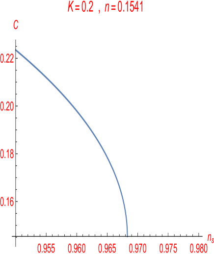
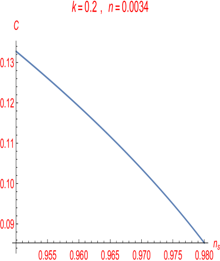
Also, here we use equation (25) and second swampland condition (4), we obtain the values of $c^{\prime}$ in terms of the tensor to scalar ratio $r$. Now, we plot graph $c^{\prime}$ in terms of $r$, we will see how much this function changes.

Figure 2: The variation of $c^{\prime}$ in terms of parameter $r$ , K is given by Planck 2018 and the upper and lower bound of $n$ are obtained by calculation

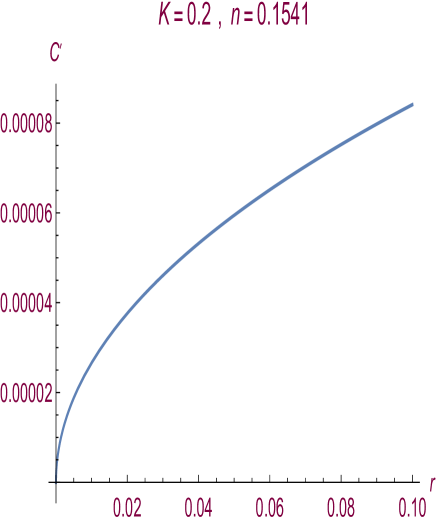
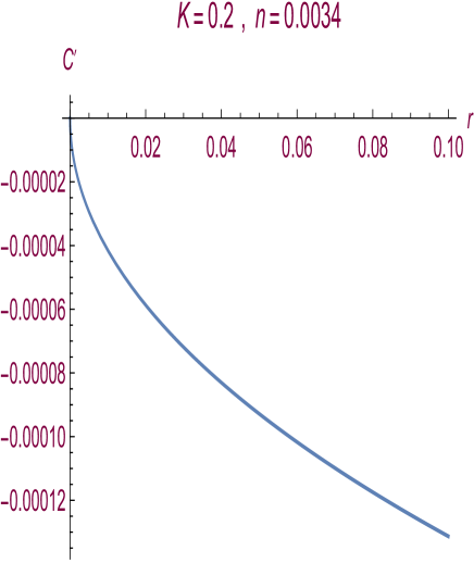
As we mentioned before we wrote tensor to scalar ratio $r$ in terms of field in equation (25) and combined the corresponding equation with second swampland condition (4). So, we obtained the values of $c^{\prime}$ in terms of the tensor to scalar ratio $r$, see figures $2a$ and $2b$. The figures $2a$ and $2b$ shown that the permissible values are as stated in Planck 2018.

Also next step, we rewrite tensor to scalar ratio $r$ in terms of the scalar field and combine this relation with the first swampland condition (17). So we obtain the values of $c$ in terms of the tensor to scalar ratio. Now, if we plot graph $c$ in terms of $r$, we can see how much this function changes.

Figure 3: The variation of $c$ in terms $r$ with K and $n$ (upper and lower bound) are given by Planck 2018 and calculation respectively

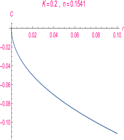
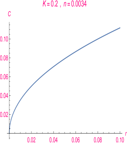
As we know in this section and previous section different swampland conditions give us different diagrams . In the following we will try to use relation between cosmological parameters as discussed before, namely the scalar spectral index and the tensor to scalar ratio. So, in order to show that our result match to plank 2018 data, next step one can draw the variation $n_{s}$ in terms of $r$.

Figure 4: We have plotted the variation of $n_{s}$ in terms of $r$.

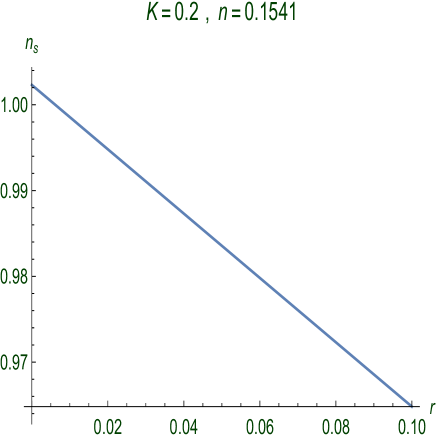
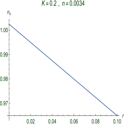
Here, by using the equations (3), (4) and (24) we obtain another constraint on the inflaton field. In that case we calculate $c^{2}c^{\prime 2}$ and see how the $c$ change according to different values of $c^{\prime}$.

Figure 5: We have plotted the values of $c$ with respect to $c^{\prime}$ with given variables $n$.

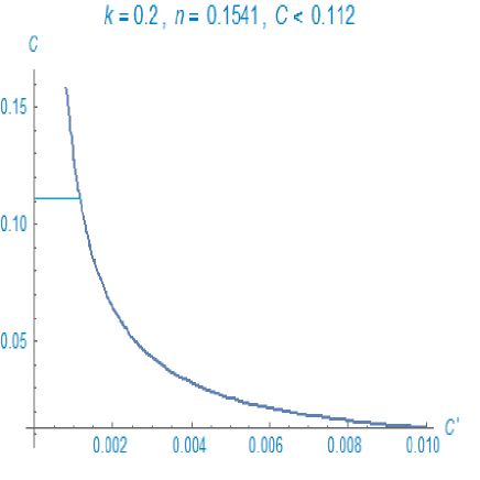
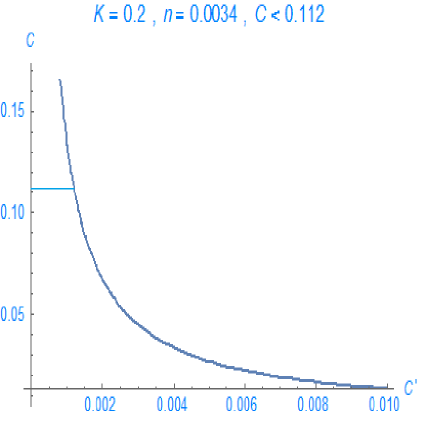
The $K$ is given Plank 2018, and $n$ known upper and lower bound. In that case our permissible values are as stated in Planck 2018, as shown in the figure $5a$ and $5b$ according to the condition $f(n)\gg(c^{2})(c^{\prime 2})$ with corresponding $n$ the permissible limit for the swampland condition is $c\ll 0,112$. Two corresponding figure as $5a$ and $5b$ complectly are satisfied by the condition of $c\ll 0,112$. Here, we mention that for the obtaining the $c\ll 0,112$, we used before equations $(24)$, $(25)$ and $(17)$. So genially one can say that the results from calculation and figures cover each other. By using mentioned values $n$ and $n_{s}$ , the permissible range $c$ and $c^{\prime}$ are specified by the corresponding figures.

5 The calculation of upper bound $n$, $\alpha$, $\beta$ and $\gamma$ coefficients theory

In order to study n, $\alpha$, $\beta$ and $\gamma$ coefficients, we use the swampland distance conjecture equation $(1)$, $(17)$ and $(24)$. On the other hand, the value of $|\Delta\varphi|\sim 1$ for different values of $n$ and $n_{s}=0.9649$, the first swampland condition must be satisfied by following relation.

$$\Delta u\simeq u$$ (26)

Now, we use the above equation about scalar spectral index and tensor to scalar ratio. In that case, we employ the value of $n_{s}$ from plank 2018 data and put the equation $(17)$, and obtain the upper bound of $n$. We achieved the different value with respect to the available equation for $n$. The most of results are satisfied by the above mentioned $n$ as $n=0.1541$. We note here, the upper and lower limit of value of $n$, the relation of $n_{s}$ and $r$ help to compute $\alpha$, $\beta$ and $\gamma$ coefficients of the corresponding theory. The coefficients are arranged with upper limit of $n$ and $n_{s}$ (from plank 2018) by the following table.

Figure 6: The values of the coefficients obtained for $n$ and $n_{s}$. (Different values have been calculated for these coefficients with respect to the two above parameters, we have selected only a few of these permissible values between zero and one).

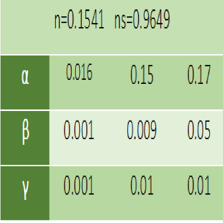
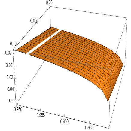
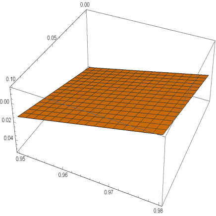
So, the above calculation lead us to show different value of coefficients in table $6$. Generally, we obtain different coefficients and we only keep some values between zero and one. Because, some physical arguments and obtained results from literature give us opportunity to keep such values[39, 40]. We note here, the first swampland condition satisfied by $c\simeq 1$. But, here the suitable coefficients $\alpha$, $\beta$ and $\gamma$ , $n$, some 2018 plank data and information from mentioned figures about $f(R)$ theory lead us to obtain approximately values for $c$ as $0.11$ (upper bound of $n$). This corresponding $c$ are completely satisfied by Ref.s.[39, 40]. Finally, we check all values obtained for $n$, $n_{s}$ and $r$ in figure(7). In fig (7a), we take $n=0.1541$ and see the variation of $n_{s}$ and $r$ with respect to corresponding $n$.

Figure 7: We have plotted the graph above using the permissible values of the parameters $n$, $r$ and $n_{s}$ expressed by the relationships. Which shows well the range of our guess.$7a:n=0.1541$ and $7b:n=0.0034$

6 Conclusions

Recently specific conditions such as the swampland condition are used to investigate the low-energy theories. So, we took advantage from that conjecture to study $f(R)$ theory. So, first we introduced inflation model with its own function, which is a polynomial plus a logarithmic terms. In that case we used Einstein Hilbert’s action and calculated the scalar field and the canonical normalization potential. We also here examined a number of cosmological parameters and investigated the validity $f(R)$ theory. By using scalar spectral index, tensor to scalar ratios and slow roll relations we also examined the validity of the swampland condition. And we show that our inflation model is consistent with the swampland conjecture. In that case, we used equations (24) and (25) with respect to 2018 planck data and obtained the upper and lower bound of $n$ as 0.15 and 0.0033. We adjusted our computational values to Planck’s values of 2018 and finally calculated each of the coefficients $\alpha$, $\beta$ and $\gamma$ with respect to the upper limit $n$ for the corresponding model. It may be interesting to investigate the swampland conjecture to the corresponding model with constant-roll instead of slow-roll conation.

References

- [1] E. Palti, The swampland: Introduction and review, Fortsch. Phys. 67, 6, 1900037 (2019).
- [2] N. A. Hamed, L. Motl and A. Nicolis, The string landscape, black holes and gravity as the weakest force, JHEP 0706, 060 (2007).
- [3] A. Medved, An Implication of ’Gravity as the weakest force, Mod. Phys. Lett. A, 22, 2605-2610 (2007).
- [4] A. Urbano, Towards a proof of the weak gravity conjecture, arxiv: 1810.05621 (2018).
- [5] Y. Akrami, R. Kallosh, A. Linde and V. Vardanyan, The landscape, the swampland and the era of precision cosmology, Fortsch. Phys. 67, no.1-2, 1800075 (2019).
- [6] T. Brennan, F.Carta and C. Vafa, The string landscape, the swampland, and the missing corner, PoS TASI2017, 015 (2017).
- [7] Ch. Lin, Type I hilltop inflation and the refined swampland criteria, Phys. Rev. D, 99, 023519 (2019).
- [8] H. Murayama, M. Yamazaki and T. Yanagida, Do we live in the swampland? JHEP 12, 032 (2018).
- [9] C. Vafa, The String landscape and the swampland, arxiv:/hep-th/0509212v2 (2005).
- [10] K. S. Garg, Ch. Krishnan and M. Zaid, Bounds on slow roll at the boundary of the landscape, JHEB 03, 029 (2019).
- [11] K. S. Garg, Ch. Krishnan and M. Zaid, Bounds on slow roll and the de Sitter swampland, arxiv:1807.05193 (2018).
- [12] S. Das, Note on single-field inflation and the swampland criteria, Phys. Rev. D, 99, 083510 (2019).
- [13] E. V. Linder and R. J. Scherrer, Aetherizing Lambda: barotropic fluids as dark energy, Phys. Rev. D, 80, 023008 (2009).
- [14] O. G. Huang, A polynomial f(R) inflation model, JCAP 1402, 035 (2019).
- [15] H. Matsui and F. Takahashi, Eternal inflation and swampland conjectures, Phys. Rev. D, 99, 023533 (2019).
-
[16]
W. Kinney, Eternal inflation and the refined swampland conjecture, Phys. Rev. Lett. 122, 081302 (2019).
William Kinney, Sunny Vagnozzi and Luca Visinelli, The zoo plot meets the swampland: mutual (in)consistency of single-field inflation, string conjectures, and cosmological data, Class. Quant. Grav. 36, 117001 (2019).
- [17] R. Schimmrigk, The Swampland spectrum conjecture in inflation, arxiv:1810.11699 (2018).
- [18] D. Cheong, S. Lee and S. C. Park, Higgs inflation and the refined dS conjecture, Phys. Lett. B, 789, 336–340 (2018)
- [19] Z. Yi and Y. Gong, Gauss-Bonnet inflation and swampland, arxiv:1811.01625 (2018).
- [20] M. Artymowski and I. Ben-Dayan, f(R) and Brans-Dicke theories and the swampland, JCAP 1905, 042 (2019).
- [21] S. Brahma and M. Hossain, Avoiding the string swampland in single-field inflation: Excited initial state, JHEP 2019, 6 (2019).
- [22] H. Ooguri, E. Palti, G. Shiu and C. Vafa, Distance and de Sitter conjectures on the swampland, Phys. Lett. B, 788, 180–184 (2019).
- [23] S. Dutta, E. Saridakis and R. Scherrer, Dark energy from a quintessence (phantom) field rolling near potential minimum (maximum). Phys. Rev. D, 79, 103005 (2009).
- [24] S. Capozziello, S. Carloni and A. Troisi, Quintessence without scalar fields, Recent Res. Dev. Astron. Astrophys 1, 625 (2003).
- [25] S. M. Carroll, V. Duvvuri, M.Trodden and M. Turner, Is cosmic speed - up due to new gravitational physics? Phys. Rev. D, 70, 043528 (2004).
- [26] Sh. Nojiri and S. Odintsov, Modified gravity with negative and positive powers of the curvature: Unification of the inflation and of the cosmic acceleration, Phys. Rev. D, 68, 123512 (2003)
- [27] A. A. Starobinsky, A new type of isotropic cosmological models without singularity, Phys. Lett. B, 91, 99 - 102 (1980).
- [28] A. Codello, J. Joergensen, F. Sannino and O. Svendsen, Marginally deformed Starobinsky gravity, JHEP 02, 050 (2015).
[29]
M. Orellana, F. Garcia, F. Teppa Pannia and G. Romero, Structure of neutron stars in -squared gravity, Gen. Rel. Grav 45, 771-783 (2013).
S. Nojiri and S. D. Odintsov, Unified cosmic history in modified gravity: from F(R) theory to Lorentz non-invariant models, Phys. Rept.505,59 (2011).
S. Capozziello, M. De Laurentis, S. D. Odintsov and A. Stabile, Hydrostatic equilibrium and stellar structure in f(R)-gravity, Phys. Rev. D 83, 064004 (2011).
Salvatore Capozziello, Mir. Faizal, Mir. Hameeda, Behnam Pourhassan, Vincenzo Salzano and Sudhaker Upadhyay, Clustering of Galaxies with f(R) gravity, Mon. Not. Roy. Astron. Soc. 474, 2430-2443 (2018). -
[30]
A. Arapoglu, C. Deliduman and K. Y. Eksi, Constraints on perturbative f(R) gravity via neutron Stars, JCAP 1107, 020 (2011).
S. Capozziello, R. D’Agostino, O. Luongo, Extended Gravity Cosmography, Int. J. Mod. Phys. D, 28, 1930016 (2019).
S. Capozziello, R. D’Agostino, O. Luongo, Rational approximations of f(R) cosmography through Padé polynomials, JCAP 1805, 008 (2018).
M. Khurshudyan, A. Pasqua, and B. Pourhassan, Higher derivative corrections of gravity with varying equation of state in the case of variable and , Can. J. Phys. 1107, 449-455 (2015). -
[31]
Ph. Channuie, Deformed Starobinsky model in gravity’s rainbow, Eur. Phys. J. C, 79, 508 (2019).
S. Capozziello, R. D’Agostino, O. Luongo, Kinematic model-independent reconstruction of Palatini f(R) cosmology, Gen. Rel. Grav. 51, 2 (2019).
S. Nojiri, S. D. Odintsov and V. K. Oikonomou, Modified gravity theories on a nutshell: inflation, bounce and late-time evolution, Phys. Rept. 692, 1 (2017).
R. Myrzakulov, L. Sebastian and S. Vagnozzi, Inflation in -theories and mimetic gravity scenario, Eur. Phys. J.C 75, 444 (2015). -
[32]
J. Sadeghi, B. Pourhassan, A. S. Kubeka and M. Rostami, Logarithmic corrected Polynomial inflation mimicking a cosmological constant, Int. J. Mod. PhysD, 25, 1650077. (2015).
S. Nojiri and S. D. Odintsov, Modified gravity with ln R terms and cosmic acceleration, Gen. Rel. Grav. 36, 1765 (2004).
S. D. Odintsov, V. K. Oikonomou and L. Sebastiani, Unification of constant-roll iInflation and dark energy with logarithmic -corrected and exponential gravity, Nucl. Phys. B, 923, 608 (2017).
E. Elizalde, S. D. Odintsov, L. Sebastiani and R. Myrzakulov, Beyond-one-loop quantum gravity action yielding both inflation and late-time acceleration, Nucl. Phys. B, 921,411 (2017). -
[33]
A. A. Starobinsky, Disappearing cosmological constant in f(R) gravity, JETP. Lett 86, 157-163 (2007).
E. Elizalde, S. D. Odintsov, V. K. Oikonomou and T. Paul, Logarithmic-corrected gravity inflation in the presence of Kalb-Ramond fields, JCAP 1902, 017 (2019).
Channuie. Phongpichit, Refined swampland conjecture in deformed Starobinsky gravity, arxiv:1907.10605 (2019). - [34] H. Alavirad and J. Weller, Modified gravity with logarithmic curvature corrections and the structure of relativistic stars, Phys. Rev. D, 88, 124034 (2013).
- [35] T. Saidov and A. Zhuk, Bouncing inflation in nonlinear gravitational model, IPhys. Rev. D, 81, 124002 (2010).
- [36] G. Magnano and L. Sokolowski, On physical equivalence between nonlinear gravity theories and a general relativistic selfgravitating scalar field, Phys. Rev. D, 50, 5039-5059 (1994).
- [37] A. Liddle and R. Scherrer, A classification of scalar field potentials with cosmological scaling solutions, Phys. Rev.D, 59, 023509 (1999).
- [38] A. Albrecht and P. Steinhardt, Cosmology for grand unified theories with radiatively induced symmetry breaking, Phys. Rev. Lett. 48, 1220-1223 (1982).
- [39] A. Kehagias and A. Riotto, A note on inflation and the swampland, Fortsch. Phys 66, 1800052 (2018).
- [40] Y. Akrami and others, Planck 2018 results. X. Constraints on inflation, arxiv:1807.06211 (2018).
- [41] L. Amendola, Coupled quintessence, Phys. Rev. D, 62, 043511 (2000).
- [42] P. Agrawal, G.Obied, P. Steinhardt and C. Vafa, On the cosmological implications of the string swampland, Phys. Lett. B, 784, 271–276 (2018).