SPICE: Self-supervised Pitch Estimation

Abstract

We propose a model to estimate the fundamental frequency in monophonic audio, often referred to as pitch estimation. We acknowledge the fact that obtaining ground truth annotations at the required temporal and frequency resolution is a particularly daunting task. Therefore, we propose to adopt a self-supervised learning technique, which is able to estimate pitch without any form of supervision. The key observation is that pitch shift maps to a simple translation when the audio signal is analysed through the lens of the constant-Q transform (CQT). We design a self-supervised task by feeding two shifted slices of the CQT to the same convolutional encoder, and require that the difference in the outputs is proportional to the corresponding difference in pitch. In addition, we introduce a small model head on top of the encoder, which is able to determine the confidence of the pitch estimate, so as to distinguish between voiced and unvoiced audio. Our results show that the proposed method is able to estimate pitch at a level of accuracy comparable to fully supervised models, both on clean and noisy audio samples, although it does not require access to large labeled datasets.

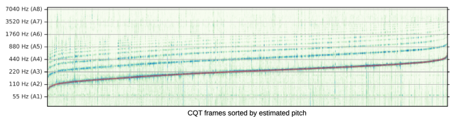
Figure 1: CQT frames extracted from the MIR-1k dataset re-ordered based on the pitch estimated by the SPICE algorithm (in red).

I Introduction

Pitch represents a perceptual property of sound which is relative, since it allows ordering to distinguish between high and low sounds, intensive, that is, mixing sources with different pitches produces a chord, not a single unified tone – contrary to loudness, which is additive in the number of sources, and it is a property that can be attributed to a sound independently of its source [1]. For example, the note A4 is perceived as the same pitch whether it is played on a guitar or on a piano. A comprehensive treatment of the psychoacoustic aspects of pitch perception is given in [2]. Pitch often corresponds to the fundamental frequency ($f_{0}$), i.e., the frequency of the lowest harmonic. However, the former is a perceptual property, while the latter is a physical property of the underlying audio signal. While there are a few notable exceptions (e.g., the Shepard tone, the tritone paradox, or the auditory illusions described in [3]), this correspondence holds for the broad class of locally periodic signals, which represents a good abstraction for the audio signals considered in this paper.

Pitch estimation in monophonic audio received a great deal of attention over the past decades, due to its central importance in several domains, ranging from music information retrieval to speech analysis. Traditionally, simple signal processing pipelines were proposed, working either in the time domain [4, 5, 6, 7], in the frequency domain [8] or both [9, 10], often followed by post-processing algorithms to smooth the pitch trajectories [11, 12]. Until recently, machine learning methods had not been able to outperform hand-crafted signal processing pipelines targeting pitch estimation. This was due to the lack of annotated data, which is particularly tedious and difficult to obtain at the temporal and frequency resolution required to train fully supervised models. To overcome these limitations, a synthetically generated dataset was proposed in [13], obtained by re-synthesizing monophonic music tracks while setting the fundamental frequency to the target ground truth. Using this training data, the CREPE algorithm [14] was able to achieve state-of-the-art results when evaluated on the same dataset, outperforming signal processing baselines, especially under noisy conditions.

In this paper we address the problem of lack of annotated data from a different angle. Specifically, we rely on self-supervision, i.e., we define an auxiliary task (also known as a pretext task) which can be learned in a completely unsupervised way. To devise this task, we started from the observation that for humans, including professional musicians, it is typically much easier to estimate relative pitch, related to the frequency interval between two notes, than absolute pitch, related to the actual fundamental frequency [15]. Therefore, we design SPICE (Self-supervised PItCh Estimation) to solve a similar task. More precisely, our network architecture consists of a convolutional encoder which produces a single scalar embedding. We aim at learning a model that linearly maps this scalar value to pitch, when the latter is expressed in a logarithmic scale, i.e., in units of semitones of an equally tempered chromatic scale. To do this, we feed two versions of the same signal to the encoder, one being a pitch shifted version of the other by a random but known amount. Then, we devise a loss function that forces the difference between the scalar embeddings to be proportional to the known difference in pitch. Upon convergence, the model is able to estimate relative pitch, solely relying on self-supervision. In order to translate relative pitch to absolute pitch, we apply a simple calibration step, which can be done using a small synthetically generated dataset. Therefore, the model is able to produce absolute pitch without having access to any manually labelled dataset.

A key characteristic of our model is that it receives as input a signal transformed in the domain defined by the constant-Q transform (CQT), which represents a convenient choice for analysing pitch. Indeed, the CQT filter bank computes a wavelet transform [16], and wavelets can be effectively used to represent the class of locally periodic signals. When the number of filters per octave (also known as quality factor) is large enough, wavelets have a discernible pitch which is related to the logarithm of the scale variable. For this reason, pitch shifting can be conveniently expressed as a simple translation along the log-spaced frequency axis induced by the CQT. Note that this property holds also for inharmonic or noisy audio signals for which the fundamental frequency cannot be defined. For example, stretching these signals in time produces a sensation of pitch shift, which would be observable in the CQT domain despite the absence of the fundamental frequency. Conversely, we acknowledge the fact that for some specific audio signals the analysis in the CQT domain might lead to erroneous pitch estimates. For example, if the input signal is a Shepard tone and the amount of pitch shift is equal to +11 semitones, the human ear would perceive a pitch interval of -1 semitone. Hence, both the magnitude and the sign of the estimated pitch would be incorrect. Despite the existence of these handcrafted examples for which our approach does not apply, the correspondence between pitch shift and translation in the CQT domain still holds for most real-world audio signals used to train and evaluate our model.

Another important aspect of pitch estimation is determining whether the underlying signal is voiced or unvoiced. Instead of relying on handcrafted thresholding mechanisms, we augment the model in such a way that it can learn the level of confidence of the pitch estimation. Namely, we add a simple fully connected layer that receives as input the penultimate layer of the encoder and produces a second scalar value which is trained to match the pitch estimation error.

In summary, this paper makes the following key contributions:

• We propose a self-supervised pitch estimation model, which can be trained without having access to any labelled dataset.

• We incorporate a self-supervised mechanism to estimate the confidence of the pitch estimation, which can be directly used for voicing detection.

• We evaluate our model against two publicly available monophonic datasets and show that in both cases we outperform handcrafted baselines, while matching the level of accuracy attained by CREPE, despite having no access to ground truth labels.

• We train and evaluate our model also in the noisy conditions, where background music is present in addition to monophonic singing, and show that also in this case, match the level of accuracy obtained by CREPE.

As an illustration, Figure 1 shows the CQT frames of one of the evaluation datasets (MIR-1k [17]), which are considered to be voiced. The red solid line represents pitch as estimated by the SPICE and the CQT frames are sorted according to this value from low to high pitch.

The rest of this paper is organized as follows. Section II contrasts the proposed method against the existing literature. Section III illustrates the proposed method, which is evaluated in Section IV. Conclusions and future remarks are discussed in Section V.

II Related work

Pitch estimation: Traditional pitch estimation algorithms are based on hand-crafted signal processing pipelines, working in the time and/or frequency domain. The most common time-domain methods are based on the analysis of local maxima of the auto-correlation function (ACF) [4]. These approaches are known to be prone to octave errors, because the peaks of the ACF repeat at different lags. Therefore, several methods were introduced to be more robust to such errors, including, e.g., the PRAAT [5] and RAPT [6] algorithms. An alternative approach is pursued by the YIN algorithm [7], which looks for the local minima of the Normalized Mean Difference Function (NMDF), to avoid octave errors caused by signal amplitude changes. Different frequency-domain methods were also proposed, based, e.g., on spectral peak picking [18] or template matching with the spectrum of a sawtooth waveform [8]. Other approaches combine both time-domain and frequency-domain processing, like the Aurora algorithm [9] and the nearly defect-free F0 estimation algorithm [10]. Comparative analyses including most of the aforementioned approaches have been conducted on speech [19, 20], singing voices [21] and musical instruments [22]. Machine learning models for pitch estimation in speech were proposed in [23, 24]. The method in  [23] first extracts hand-crafted spectral domain features, and then adopts a neural network (either a multi-layer perceptron or a recurrent neural network) to compute the estimated pitch. In [24] consensus of other pitch trackers is used to get ground truth, and a multi-layer perceptron classifier is trained on the principal components of the autocorrelations of subbands from an auditory filterbank. More recently the CREPE [14] model was proposed, an end-to-end convolutional neural network which consumes audio directly in the time domain. The network is trained in a fully supervised fashion, minimizing the cross-entropy loss between the ground truth pitch annotations and the output of the model. In our experiments, we compare our results with CREPE, which is the current state-of-the-art.

Pitch confidence estimation: Most of the aforementioned methods also provide a voiced/unvoiced decision, often based on heuristic thresholds applied to hand-crafted features. However, the confidence of the estimated pitch in the voiced case is seldom provided. A few exceptions are CREPE [14], which produces a confidence score computed from the activations of the last layer of the model, and [25], which directly addresses this problem, by training a neural network based on hand-crafted features to estimate the confidence of the estimated pitch. In contrast, in our work we explicitly augment the proposed model with a head aimed at estimating confidence in a fully unsupervised way.

Pitch tracking and polyphonic audio: Often, post-processing is applied to raw pitch estimates to smoothly track pitch contours over time. For example,  [26] applies Kalman filtering to smooth the output of a hybrid spectro-temporal autocorrelation method, while the pYIN algorithm [11] builds on top of YIN, by applying Viterbi decoding of a sequence soft pitch candidates. A similar smoothing algorithm is also used in the publicly released version of CREPE [14]. Pitch extraction in the case of polyphonic audio remains an open research problem [27]. In this case, pitch tracking is even more important to be able to distinguish the different melody lines [12]. A machine learning model targeting the estimation of multiple fundamental frequencies, melody, vocal and bass line was recently proposed in [28] .

Self-supervised learning: The widespread success of fully supervised models was stimulated by the availability of annotated datasets. In those cases in which labels are scarse or simply not available, self-supervised learning has emerged as a promising approach for pre-training deep convolutional networks both for vision [29, 30, 31] and audio-related tasks [32, 33, 34]. Somewhat related to our paper are those methods that try to use self-supervision to obtain point disparities between pairs of images [35], where shifts in the spatial domain play the role of shifts in the log-frequency domain.

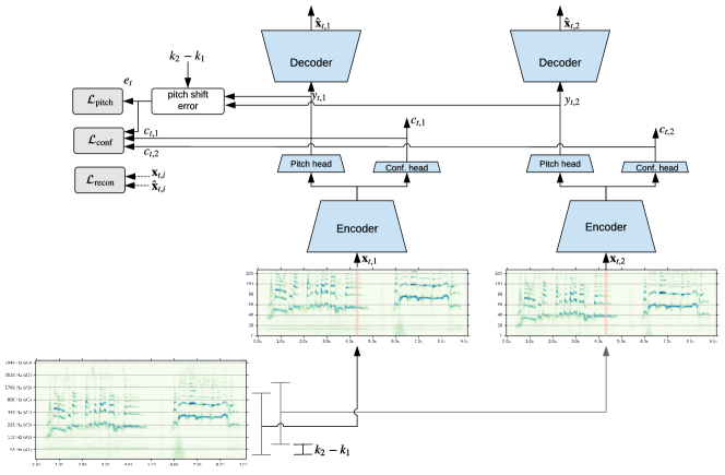
Figure 2: SPICE model architecture.

III Methods

The proposed pitch estimation model receives as input an audio track of arbitrary length and produces as output a time series of estimated pitch frequencies, together with an indication of the confidence of the estimates. The latter is used to discriminate between unvoiced frames, in which pitch is not well defined, and voiced frames.

Audio frontend

Our proposed model does not consume audio directly, but instead it receives as input individual frames of the constant-Q transform (CQT). As illustrated in [16], the CQT representation approximately corresponds to the output of a wavelet filter bank defined by the following family of wavelets:

$$\psi_{\lambda_{k}}(t)=\lambda_{k}\psi(\lambda_{k}t),$$ (1)

where $Q$ denotes the number of filters per octave and

$$\lambda_{k}=f_{base}2^{\frac{k}{Q}},\quad k\in 0,\ldots,F_{\text{max}}-1,$$ (2)

where $f_{base}$ is the frequency of the lowest frequency bin and $F_{\text{max}}$ is the number of CQT bins. The Fourier transform of the wavelet filters can be expressed as:

$$\Psi_{\lambda_{k}}=\Psi\left(\frac{f}{\lambda_{k}}\right)$$ (3)

Assuming that the center frequency of $\Psi(f)$ is normalized to 1, each filter is centered at frequency $\lambda_{k}$ and has a bandwidth equal to $\lambda_{k}/Q$. Hence, if we consider two filters with indices $k_{1}$ and $k_{2}$, one of the corresponding wavelets would the pitch-shifted version of the other. That is,

$$\Delta k=k_{2}-k_{1}=Q\cdot\log_{2}\alpha,$$ (4)

where $\alpha=\lambda_{k_{2}}/\lambda_{k_{1}}$. Therefore, for the class of locally periodic signals that can be represented as a wavelet expansion, a translation of $\Delta k$ bins in the CQT domain is related to a pitch-shift by a factor $\alpha$.

Note that this key property of mapping pitch-shift to a simple translation does not hold in general for other audio frontends, e.g., for the widely used mel spectrogram. In this case, the relationship between frequency (in Hz) and mel units is given by

$$m=c\cdot\log\left(1+\frac{f}{f_{\text{break}}}\right)$$ (5)

for some constants $c$ and $f_{\text{break}}$ (also known as break frequency). Hence, the relationship is approximately linear at low frequencies ($f\ll f_{\text{break}}$) and logarithmic at high frequencies ($f\gg f_{\text{break}}$), with a smooth transition between these two regimes. It is straightforward to show that a multiplicative scaling of frequencies does not correspond to an additive scaling in the mel domain.

Pitch estimation

The proposed model architecture is illustrated in Figure 2. Given an input track, the audio frontend computes the absolute value of the CQT, which is represented as a real-valued matrix $X$ of size $T\times F_{\text{max}}$, where $T$ depends on the selected hop length. From each temporal frame $t=1,\ldots,T$ (where $T$ is equal to the batch size during training) the model samples at random two integer offsets $k_{t,1}$ and $k_{t,2}$ from a uniform distribution, i.e., $k_{t,i}\sim\mathcal{U}(k_{\text{min}},k_{\text{max}}$), and it extracts two corresponding slices $\mathbf{x}_{t,1},\mathbf{x}_{t,2}\in\mathbb{R}^{F}$, spanning the range of CQT bins $[k_{t,i},k_{t,i}+F]$, $i=1,2$, where $F$ is the number of CQT bins in the slice. Then, each vector is fed to the same encoder to produce a single scalar $y_{t,i}=Enc(x_{t,i})\in\mathbb{R}$. The encoder is a neural network with $L$ convolutional layers followed by two fully-connected layers. Further details about the model architecture are provided in Section IV.

We design our main loss in such a way that $y_{t,i}$ is encouraged to encode pitch. First, we define the relative pitch error as

$$e_{t}=|(y_{t,1}-y_{t,2})-\sigma(k_{t,1}-k_{t,2})|$$ (6)

Then, the loss is defined as the Huber norm [36] of the pitch error:

$$\mathcal{L}_{\text{pitch}}=\frac{1}{T}\sum_{t}h(e_{t}),$$ (7)

where:

$$h(x)=\begin{cases}\frac{\mathbf{x}^{2}}{2},\quad|x|\leq\tau\\ \frac{\tau^{2}}{2}+\tau(|x|-\tau),\quad\text{otherwise.}\\ \end{cases}$$ (8)

The pitch difference scaling factor $\sigma$ is adjusted in such a way that $y_{t}\in[0,1]$ when pitch is in the range $[f_{\text{min}},f_{\text{max}}]$, namely:

$$\sigma=\frac{1}{Q\cdot\log_{2}(f_{\max}/f_{\min})}$$ (9)

The values of $f_{\min}$ and $f_{\max}$ are determined based on the range of pitch frequencies spanned by the training set. In our experiments we found that the Huber loss makes the model less sensitive to the presence of unvoiced frames in the training dataset, for which the relative pitch error can be large, as pitch is not well defined in this case.

In addition to $\mathcal{L}_{\text{pitch}}$, we also use the following reconstruction loss

$$\mathcal{L}_{\text{recon}}=\frac{1}{T}\sum_{t}\|\mathbf{x}_{t,1}-\hat{\mathbf{x}}_{t,1}\|_{2}^{2}+\|\mathbf{x}_{t,2}-\hat{\mathbf{x}}_{t,2}\|_{2}^{2},$$ (10)

where $\hat{\mathbf{x}}_{t,i}$, $i=1,2$, is a reconstruction of the input frame obtained by feeding $y_{i,t}$ into a decoder $\hat{\mathbf{x}}_{t,i}=Dec(y_{i,t})$. The reconstruction loss $\mathcal{L}_{\text{recon}}$ forces the reconstructed frame $\hat{\mathbf{x}}_{t,i}$ to be as close as possible to the original frame $\mathbf{x}_{t,i}$. The decoder is a neural network with $L$ convolutional layers whose architecture is the mirrored version of the encoder, with convolutions replaced by transposed convolutions, which maps the scalar value $y_{i,t}$ back to a vector with the same shape as the input frame. Further details about the model architecture are provided in Section IV. In Section IV we also empirically evaluate the impact of this loss component as part of the ablation study.

Therefore, the overall loss is defined as:

$$\mathcal{L}=w_{\text{pitch}}\mathcal{L}_{\text{pitch}}+w_{\text{recon}}\mathcal{L}_{\text{recon}},$$ (11)

where $w_{\text{pitch}}$ and $w_{\text{recon}}$ are scalar weights that determine the relative importance assigned to the two loss components.

Given the way it is designed, the proposed model can only estimate relative pitch differences. The absolute pitch of an input frame is obtained by applying an affine mapping:

$$\hat{p}_{0,t}=b+s\cdot y_{t}=b+s\cdot Enc(\mathbf{x}_{t})\quad[\text{semitones}],$$ (12)

which depends on two parameters. This is needed to map the output of the encoder $y_{t}$ from the $[0,1]$ range to the absolute pitch range (expressed in semitones). We use a small amount of synthetically generated data (locally periodic signals with a known frequency) to estimate both the intercept $\hat{b}$ and the slope $\hat{s}$. More specifically, we generate a waveform which is piece-wise harmonic and consists of $M$ pieces. Each piece is a purely harmonic signal with fundamental frequency $f_{0}$ corresponding to a semitone sampled uniformly at random in the range A2 (110Hz) and A4 (440Hz). We sample the amplitude of the first harmonic in $a_{0}\sim\mathcal{N}(0,1)$ and that of higher order harmonics in $a_{k}\sim a_{0}\cdot\mathcal{U}(0,1)$, $k=1,\ldots,K$. A random phase is applied to each harmonic. In our experiments, each piece is $N\cdot H$ samples long, where $H$ denotes the CQT hop-length used by the SPICE model and $N$ the number of frames. We feed this waveform to SPICE and consider the estimate produced for the central frame in each piece (to mitigate errors due to boundary effects). This leads to $M$ synthetically generated samples that can be used to fit the model in (12). In Section IV we empirically evaluate the robustness of the calibration process for different values of $M$.

Note that pitch in (12) is expressed in semitones and it can be converted to frequency (in Hz) by:

$$\hat{f}_{0,t}=f_{base}2^{\frac{\hat{p}_{0,t}}{12}}\quad[\text{Hz}]$$ (13)

Confidence estimation

In addition to the estimated pitch $\hat{p}_{0,t}$, we design our model such that it also produces a confidence level $c_{t}\in[0,1]$. Indeed, when the input audio is voiced we expect to produce high confidence estimates, while when it is unvoiced pitch is not well defined and the output confidence should be low. To achieve this, we design the encoder architecture to have two heads on top of the convolutional layers, as illustrated in Figure 2. The first head consists of two fully-connected layers and produces the pitch estimate $y_{t}$. The second head consists of a single fully-connected layer and produces the confidence level $c_{t}$. To train the latter, we add the following loss:

$$\mathcal{L}_{\text{conf}}=\frac{1}{T}\sum_{t}|(1-c_{t,1})-e_{t}/\sigma|^{2}+|(1-c_{t,2})-e_{t}/\sigma|^{2}.$$ (14)

This way the model will produce high confidence $c_{t}\sim 1$ when the model is able to correctly estimate the pitch difference between the two input slices. At the same time, given that our primary goal is to accurately estimate pitch, during the backpropagation step we stop the gradients so that $\mathcal{L}_{\text{conf}}$ only influences the training of the confidence head and does not affect the other layers of the encoder architecture.

TABLE I: Dataset specifications.

		Length			# of frames
Dataset	# of tracks	min	max	total	voiced	total
MIR-1k	1000	3s	12s	133m	175k	215k
MDB-stem-synth	230	2s	565s	418m	784k	1.75M
SingingVoices	88	25s	298s	185m	194k	348k

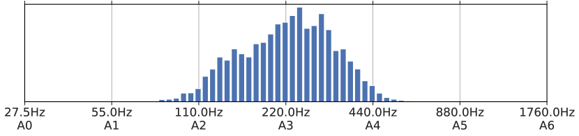
(a) MIR-1k

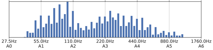
(b) MDB-stem-synth

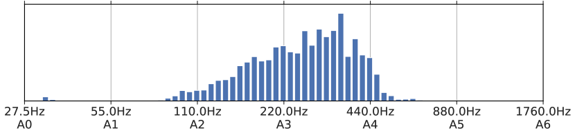
(c) SingingVoices

Figure 3: Range of pitch values covered by the different datasets.

Handling background music

The accuracy of pitch estimation can be severely affected when dealing with noisy conditions, which emerge, for example, when the singing voice is superimposed over background music. In this case, we are faced with polyphonic audio and we want the model to focus only on the singing voice source. To deal with these conditions, we introduce a data augmentation step in our training setup. More specifically, we mix the clean singing voice signal with the corresponding instrumental backing track at different levels of signal-to-noise (SNR) ratios. Interestingly, we found that simply augmenting the training data was not sufficient to achieve a good level of robustness. Instead, we also modified the definition of the loss functions as follows. Let $\mathbf{x}_{t,i}^{c}$ and $\mathbf{x}_{t,i}^{n}$ denote, respectively, the CQT of the clean and noisy input samples. Similarly, $y_{t,i}^{c}$ and $y_{t,i}^{n}$ denote the corresponding outputs of the encoder. The pitch error loss is modified by averaging four different variants of the error, that is:

$$e_{t}^{pq}=|(y_{t,1}^{p}-y_{t,2}^{q})-\sigma(k_{t,1}-k_{t,2})|\quad p,q\in\{c,n\},$$ (15)

$$\mathcal{L}_{\text{pitch}}=\frac{1}{4}\sum_{t}\sum_{p,q\in\{c,n\}}h(e_{t}^{pq}).$$ (16)

The reconstruction loss is also modified, so that the decoder is asked to reconstruct the clean samples only. That is:

$$\mathcal{L}_{\text{recon}}=\frac{1}{T}\sum_{t}\|\mathbf{x}_{t,1}^{c}-\hat{\mathbf{x}}_{t,1}\|_{2}^{2}+\|\mathbf{x}_{t,2}^{c}-\hat{\mathbf{x}}_{t,2}\|_{2}^{2}.$$ (17)

The rationale behind this approach is that the encoder is induced to represent in its output only the information relative to the clean input audio samples, thus learning to denoise the input by separating the singing voice from noise.

IV Experiments

Model parameters

First we provide the details of the default parameters used in our model. The input audio track is sampled at $16$ kHz. The CQT frontend is parametrized to use $Q=24$ bins per octave, so as to achieve a resolution equal to one half-semitone per bin. We set $f_{base}$ equal to the frequency of the note $C_{1}$, i.e., $f_{base}\simeq 32.70$ Hz and we compute up to $F_{max}=190$ CQT bins, i.e., to cover the range of frequency up to Nyquist. We use a Hann window with hop length set equal to 512 samples, i.e., one CQT frame every 32 ms. The CQT is implemented using TensorFlow operations following the specifications of the open-source librosa library [37]. During training, we extract slices of $F=128$ CQT bins, setting $k_{\text{min}}=0$ and $k_{\text{max}}=8$ (i.e., between 0 and 4 semitones when $Q=24$). The Huber threshold is set to $\tau=0.25\sigma$ and the loss weights equal to, respectively, $w_{\text{pitch}}=10^{4}$ and $w_{\text{recon}}=1$. We increased the weight of the pitch-shift loss to $w_{\text{pitch}}=3\cdot 10^{5}$ when training with background music.

The encoder receives as input a 128-dimensional vector corresponding to a sliced CQT frame and produces as output two scalars representing, respectively, pitch and confidence. The model architecture consists of $L=6$ convolutional layers. We use filters of size $3$ and stride equal to $1$. The number of channels is equal to $d\cdot[1,2,4,8,8,8]$, where $d=64$ for the encoder and $d=32$ for the decoder. Each convolution is followed by batch normalization and a ReLU non-linearity. Max-pooling of size $3$ and stride $2$ is applied at the output of each layer. Hence, after flattening the output of the last convolutional layer we obtain an embedding of size $1024$ elements. This is fed into two different heads. The pitch estimation head consists of two fully-connected layers with, respectively, 48 and 1 units. The confidence head consists of a single fully-connected layer with 1 output unit. The total number of parameters of the encoder is equal to 2.38M. Note that we do not apply any form of temporal smoothing to the output of the model.

The model is trained using Adam [38] with default hyperparameters and learning rate equal to $10^{-4}$. The batch size is set to $64$. During training, the CQT frames of the input audio tracks are shuffled, so that the frames in a batch are likely to come from different tracks.

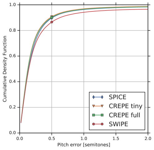
(a) MIR-1k

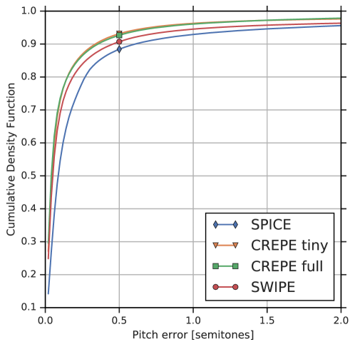
(b) MDB-stem-synth

Figure 4: Raw Pitch Accuracy.

TABLE II: Evaluation results.

			MIR-1k		MDB-stem-synth
Model	# params	Trained on	RPA (CI 95%)	VRR	RPA (CI 95%)
SWIPE	-	-	86.6%	-	90.7%
CREPE tiny	487k	many	90.7%	88.9%	93.1%
CREPE full	22.2M	many	90.1%	84.6%	92.7%
SPICE	2.38M	SingingVoices	$90.6\%\pm 0.1\%$	86.8%	$89.1\%\pm 0.4\%$
SPICE	180k	SingingVoices	$90.4\%\pm 0.1\%$	90.5%	$87.9\%\pm 0.9\%$

TABLE III: Evaluation results of the ablation study.

	MIR-1k	MDB-stem-synth
	RPA (CI 95%)	RPA (CI 95%)
SPICE baseline	$90.6\%\pm 0.1\%$	$89.1\%\pm 0.4\%$
w/o reconstruction loss	$55.9\%\pm 2.3\%$	$56.3\%\pm 2.7\%$
w/o data augmentation	$89.6\%\pm 0.2\%$	$71.1\%\pm 0.7\%$
w/ continuous pitch shift augmentation	$90.7\%\pm 0.1\%$	$87.8\%\pm 0.8\%$
w/ L2 loss	89.2$\%\pm 0.2\%$	$86.3\%\pm 0.9\%$
w/ L1 loss	$82.1\%\pm 0.7\%$	$82.3\%\pm 0.9\%$

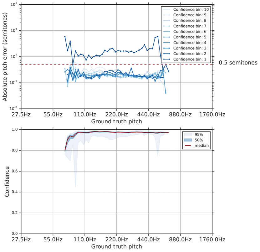
(a) SPICE

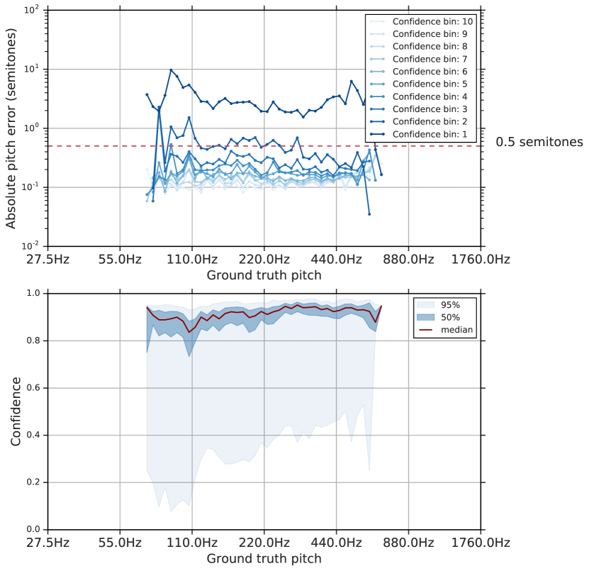
(b) CREPE full

Figure 5: Pitch error on the MIR-1k dataset, conditional on ground truth pitch and model confidence.

Datasets

We use three datasets in our experiments, whose details are summarized in Table I. The MIR-1k [17] dataset contains 1000 audio tracks with people singing Chinese pop songs. The dataset is annotated with pitch at a granularity of 10 ms and it also contains voiced/unvoiced frame annotations. It comes with two stereo channels representing, respectively, the singing voice and the accompaniment music. The MDB-stem-synth dataset [13] includes re-synthesized monophonic music played with a variety of musical instruments. This dataset was used to train the CREPE model in [14]. In this case, pitch annotations are available at a granularity of 29 ms. Given the mismatch of the sampling period of the pitch annotations across datasets, we resample the pitch time-series with a period equal to the hop length of the CQT, i.e., 32 ms. In addition to these publicly available datasets, we also collected in-house the SingingVoices dataset, which contains 88 audio tracks of people singing a variety of pop songs, for a total of 185 minutes.

Figure 3 illustrates the empirical distribution of pitch values. For SingingVoices, there are no ground-truth pitch labels, so we used the ouput of CREPE (configured with full model capacity and enabling Viterbi smoothing) as a surrogate. We observe that MDB-stem-synth spans a significantly larger range of frequencies (approx. 5 octaves) than MIR-1k and SingingVoices (approx. 3 octaves). Note that this is still smaller than the range covered by human hearing, which extends to 9-10 octaves. Further work is needed to collect datasets and evaluate pitch estimation algorithms on such a broad frequency range.

We trained SPICE using either SingingVoices or MIR-1k and used both MIR-1k (singing voice channel only) and MDB-stem-synth to evaluate models in clean conditions. To handle background music, we repeated training on MIR-1k, but this time applying data augmentation by mixing in backing tracks with a SNR uniformly sampled from [-5dB, 25dB]. For the evaluation, we used the MIR-1k dataset, mixing the available backing tracks at different levels of SNR, namely 20dB, 10dB and 0dB. In all cases, we apply data augmentation during training, by pitch-shifting the input audio tracks by an amount in semitones uniformly sampled in the discrete set $\{-12,0,+12\}$, using a TensorFlow-based implementation of the phase-vocoder algorithm in [39]. We found that this works better than sampling from a continuous set, because of the artifacts introduced by the pitch-shifting algorithm when adopting arbitrary rational scaling factors.

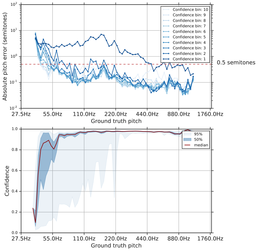
(a) SPICE

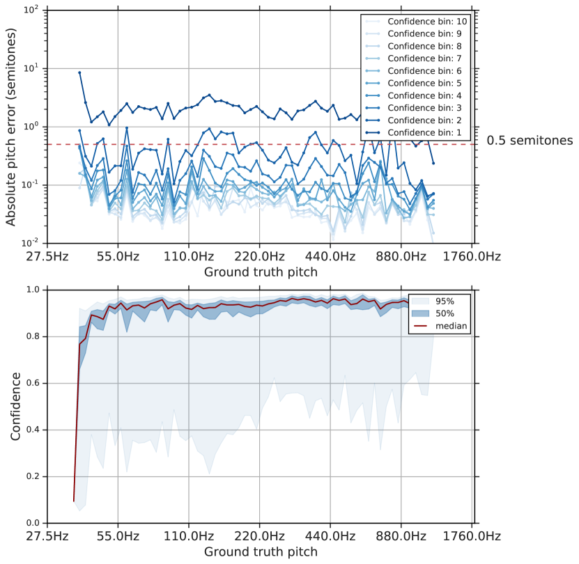
(b) CREPE full

Figure 6: Pitch error on the MDB-stem-synth dataset, conditional on ground truth pitch and model confidence.

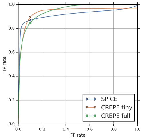
Figure 7: Voicing Detection - ROC (MIR-1k).

TABLE IV: Evaluation results on noisy datasets.

			MIR-1k
Model	# params	Trained on	clean	20dB	10dB	0dB
SWIPE	-	-	86.6%	84.3%	69.5%	27.2%
CREPE tiny	487k	many	90.7%	90.6%	88.8%	76.1%
CREPE full	22.2M	many	90.1%	90.4%	89.7%	80.8%
SPICE	2.38M	MIR-1k + augm.	$91.4\%\pm 0.1\%$	$91.2\%\pm 0.1\%$	$90.0\%\pm 0.1\%$	$81.6\%\pm 0.6\%$

Baselines

We compare our results against two baselines, namely SWIPE [8] and CREPE [14]. SWIPE estimates the pitch as the fundamental frequency of the sawtooth waveform whose spectrum best matches the spectrum of the input signal. CREPE is a data-driven method which was trained in a fully-supervised fashion on a mix of different datasets, including MDB-stem-synth [13], MIR-1k [17], Bach10 [40], RWC-Synth [11], MedleyDB [41] and NSynth [42]. We consider two variants of the CREPE model, by using model capacity tiny or full, and we disabled Viterbi smoothing, so as to evaluate the accuracy achieved on individual frames. These models have, respectively, 487k and 22.2M parameters. CREPE also produces a confidence score for each input frame.

Evaluation measures

We use the evaluation measures defined in [27] to evaluate and compare our model against the baselines. The raw pitch accuracy (RPA) is defined as the percentage of voiced frames for which the pitch error is less than 0.5 semitones. To assess the robustness of the model accuracy to the initialization, we also report the interval $\pm 2\sigma$. Here $\sigma$ is the sample standard deviation of the RPA values computed using the last 10 checkpoints of 3 separate replicas. For CREPE we do not report such interval, because we simply run the model provided by the CREPE authors on each of the evaluation datasets. The voicing recall rate (VRR) is the proportion of voiced frames in the ground truth that are recognized as voiced by the algorithm. We report the VRR at a target voicing false alarm rate equal to 10%. Note that this measure is provided only for MIR-1k, since MDB-stem-synth is a synthetic dataset and voicing can be determined based on a simple silence thresholding.

Main results

The main results of the paper are summarized in Table II and Figure 4. On the MIR-1k dataset, SPICE outperforms SWIPE, while achieving the same accuracy as CREPE in terms of RPA (90.7%), despite the fact that it was trained in an unsupervised fashion and CREPE used MIR-1k as one of the training datasets. Figure 5 illustrates a finer grained comparison between SPICE and CREPE (full model), measuring the average absolute pitch error for different values of the ground truth pitch frequency, conditioned on the level of confidence (expressed in deciles) produced by the respective algorithm. When excluding the decile with low confidence, we observe that above 110Hz, SPICE achieves an average error around 0.2-0.3 semitones, while CREPE around 0.1-0.5 semitones.

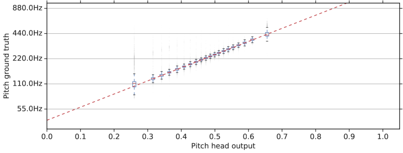
(a) MIR-1k

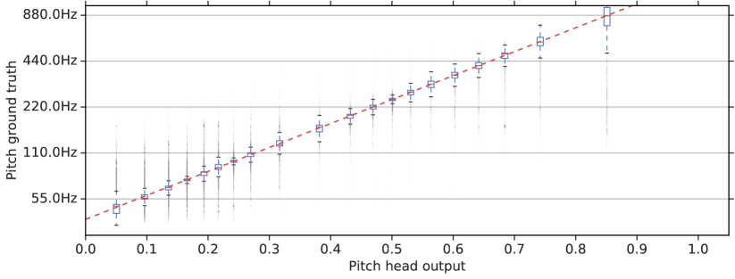
(b) MDB-stem-synth

Figure 8: Calibration of the pitch head output.

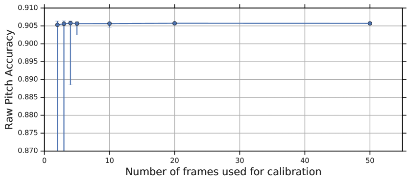
Figure 9: Robustness of the RPA on MIR-1k when varying the number of synthetically generated samples used for calibration.

We repeated our analysis on the MDB-stem-synth dataset. In this case the dataset has remarkably different characteristics from the SingingVoices dataset used for the unsupervised training of SPICE, in terms of both frequency extension (Figure 3) and timbre (singing vs. musical instruments). This explains why in this case the gap between SPICE and CREPE is wider (88.9% vs. 93.1%). Figure 6 repeats the fine-grained analysis for the MDB-stem-synth dataset, illustrating larger errors at both ends of the frequency range. We also performed a thorough error analysis, trying to understand in which cases CREPE and SWIPE outperform SPICE. We discovered that most of these errors occur in the presence of a harmonic signal, in which most of the energy is concentrated above the fifth-order harmonics, i.e., in the case of musical instruments characterized by a spectral timbre considerably different from the one of singing voice.

We also evaluated the quality of the confidence estimation comparing the voicing recall rate (VRR) of SPICE and CREPE. Results in Table II show that SPICE achieves results comparable with CREPE (86.8%, i.e., between CREPE tiny and CREPE large), while being more accurate in the more interesting low false-positive rate regime (see Figure 7).

In order to obtain a smaller, thus faster, variant of the SPICE model, we used the MorphNet [43] algorithm. Specifically, we added to the training loss (11) a regularizer which constrains the number of floating point operations (FLOPs), using $\lambda=10^{-7}$ as regularization hyper-parameter. MorphNet produces as output a slimmed network architecture, which has 180k parameters, thus more than 10 times smaller than the original model. After training this model from scratch, we were still able to achieve a level of performance on MIR-1k comparable to the larger SPICE model, as reported in Table II.

Table III shows the results of the ablation study we carried out to assess the importance of some of the design choices described in Section III. These results indicate that the reconstruction loss is crucial to obtain good results. We believe that this loss acts as a regularizer, as it enforces inputs with the same pitch but different timbre to have the same latent values. Pitch shift data augmentation is also important, especially on MDB-stem-synth, which has a wider pitch range than the training dataset (SingingVoices). Using continuous pitch shift augmentation instead of discrete octave shifts gives somewhat worse results, likely due to the artefacts it introduces. Finally, using Huber loss instead of L2 or L1 loss also gives a significant gain, which we attribute to the fact that some inputs in the data are actually unvoiced, and hence it is useful to reduce the impact of these unvoiced examples on the loss.

Table IV shows the results obtained when evaluating the models in the presence of background music. We observe that SPICE is able to achieve a level of accuracy very similar to CREPE across different values of SNR.

Calibration

The key tenet of SPICE is that is an unsupervised method. However, as discussed in Section III, the raw output of the pitch head can only represent relative pitch. To obtain absolute pitch, the intercept $b$ and the slope $s$ in (12) need to be estimated based on ground truth labels, which can be obtained using synthetically generated data without having access to any labelled dataset as described in Section III. Figure 8 shows the fitted model for both MIR-1k and MDB-stem-synth as a dashed red line. In order to quantitatively evaluate the robustness to the calibration process, we generate harmonic waveforms with $K=3$ higher-order harmonics, with $N=11$ frames and $H=512$ samples. Then, we vary the number of samples $M\in\{2,3,5,10,20,50\}$, repeat the calibration step 100 times and compute the RPA on the MIR-1k dataset. Figure 9 reports the results of this experiment (error bars represent 2.5% and 97.5% quantiles). We observe that using as few as $M=5$ synthetically generated samples are generally enough to obtain stable results.

V Conclusion

In this paper we propose SPICE, a self-supervised pitch estimation algorithm for monophonic audio. The SPICE model is trained to recognize relative pitch without access to labelled data and it can also be used to estimate absolute pitch by calibrating the model using just a few labelled examples. Our experimental results show that SPICE is competitive with CREPE, a fully-supervised model that was recently proposed in the literature, despite having no access to ground truth labels. The SPICE model is publicly available as a Tensorflow Hub module at https://tfhub.dev/google/spice/1.

References

- [1] V. Lostanlen and C.-E. Cella, “Deep Convolutional Networks on the Pitch Spiral For Music Instrument Recognition.” in ISMIR, International Society for Music Information Retrieval Conference, aug 2016.
- [2] R. F. Lyon, Human and Machine Hearing. Cambridge University Press, May 2017. [Online]. Available: https://www.cambridge.org/core/product/identifier/9781139051699/type/book
- [3] F. Esqueda, V. Välimäki, and J. Parker, “Barberpole phasing and flanging illusions,” in International Conference on Digital Audio Effects (DAFx), 2015. [Online]. Available: http://research.spa.aalto.fi/publications/
- [4] J. Dubnowski, R. Schafer, and L. Rabiner, “Real-time digital hardware pitch detector,” IEEE Transactions on Acoustics, Speech, and Signal Processing, vol. 24, no. 1, pp. 2–8, Feb 1976. [Online]. Available: http://ieeexplore.ieee.org/document/1162765/
- [5] P. Boersma and P. Boersma, “Accurate short-term analysis of the fundamental frequency and the harmonics-to-noise ratio of a sampled sound,” IFA Proceedings 17, pp. 97—-110, 1993. [Online]. Available: http://citeseerx.ist.psu.edu/viewdoc/summary?doi=10.1.1.218.4956
- [6] D. Talkin, “A Robust Algorithm for Pitch Tracking (RAPT),” in Speech Coding and Synthesis. Elsevier, 1995, pp. 495–518. [Online]. Available: https://www.semanticscholar.org/paper/A-Robust-Algorithm-for-Pitch-Tracking-(-RAPT-)-Talkin/f3f1d8960a6fde5bc4dc15acbfdce21cfc9b7452
- [7] A. De Cheveigné and H. Kawahara, “YIN, a fundamental frequency estimator for speech and music a),” Journal of the Acoustical Society of America, vol. 111, no. 4, pp. 1917–1930, 2002. [Online]. Available: http://audition.ens.fr/adc/pdf/2002{_}JASA{_}YIN.pdf
- [8] A. Camacho and J. G. Harris, “A sawtooth waveform inspired pitch estimator for speech and music,” The Journal of the Acoustical Society of America, vol. 124, no. 3, pp. 1638–1652, sep 2008. [Online]. Available: http://asa.scitation.org/doi/10.1121/1.2951592
- [9] T. Ramabadran, A. Sorin, M. McLaughlin, D. Chazan, D. Pearce, and R. Hoory, “The ETSI extended distributed speech recognition (DSR) standards: server-side speech reconstruction,” in ICASSP, vol. 1. IEEE, 2004, pp. I–53–6. [Online]. Available: http://ieeexplore.ieee.org/document/1325920/
- [10] H. Kawahara, A. de Cheveigné, H. Banno, T. Takahashi, and T. Irino, “Nearly defect-free F0 trajectory extraction for expressive speech modifications based on STRAIGHT,” in Interspeech, 2005, pp. 537–540. [Online]. Available: https://www.semanticscholar.org/paper/Nearly-defect-free-F0-trajectory-extraction-for-on-Kawahara-Cheveign{{́e}}/a2ea9c2c4fd250ae7051d6e76e74e950bd3bdbb2
- [11] M. Mauch and S. Dixon, “pYIN: A fundamental frequency estimator using probabilistic threshold distributions,” in ICASSP. IEEE, may 2014, pp. 659–663. [Online]. Available: http://ieeexplore.ieee.org/document/6853678/
- [12] J. Salamon and E. Gómez, “Melody Extraction from Polyphonic Music Signals using Pitch Contour Characteristics,” IEEE Transactions on Audio, Speech, and Language Processing, vol. 20, no. 6, pp. 1759 – 1770, 2012. [Online]. Available: http://www.music-ir.org/mirex/wiki/Audio
- [13] J. Salamon, R. Bittner, J. Bonada, J. J. Bosch, E. Gómez, and J. P. Bello, “An Analysis/Synthesis Framework for Automatic F0 Annotation of Multitrack Datasets,” in 18th International Society for Music Information Retrieval Conference, 2017. [Online]. Available: http://mtg.upf.edu/node/3830
- [14] J. W. Kim, J. Salamon, P. Li, and J. P. Bello, “CREPE: A Convolutional Representation for Pitch Estimation,” in ICASSP, Feb 2018. [Online]. Available: http://arxiv.org/abs/1802.06182
- [15] N. Ziv and S. Radin, “Absolute and relative pitch: Global versus local processing of chords.” Advances in cognitive psychology, vol. 10, no. 1, pp. 15–25, 2014. [Online]. Available: http://www.ncbi.nlm.nih.gov/pubmed/24855499http://www.pubmedcentral.nih.gov/articlerender.fcgi?artid=PMC3996714
- [16] J. Andén and S. Mallat, “Deep Scattering Spectrum,” IEEE Transactions on Signal Processing, Apr 2013. [Online]. Available: http://arxiv.org/abs/1304.6763http://dx.doi.org/10.1109/TSP.2014.2326991
- [17] C.-L. H. Jang and J.-S. Roger, “On the Improvement of Singing Voice Separation for Monaural Recordings Using the MIR-1K Dataset,” IEEE Transactions on Audio, Speech, and Language Processing, 2009. [Online]. Available: https://sites.google.com/site/unvoicedsoundseparation/mir-1k
- [18] P. Martin, “Comparison of pitch detection by cepstrum and spectral comb analysis,” in ICASSP, 1982, pp. 180–183.
- [19] D. Jouvet and Y. Laprie, “Performance Analysis of Several Pitch Detection Algorithms on Simulated and Real Noisy Speech Data,” in EUSIPCO, European Signal Processing Conference, 2017. [Online]. Available: http://www.speech.kth.se/snack/
- [20] S. Strömbergsson, “Today’s most frequently used F 0 estimation methods, and their accuracy in estimating male and female pitch in clean speech,” in Interspeech, 2016. [Online]. Available: http://dx.doi.org/10.21437/Interspeech.2016-240
- [21] O. Babacan, T. Drugman, N. Henrich, and T. Dutoit, “A comparative study of pitch extraction algorithms on a large variety of singing sounds,” in ICASSP, 2013, pp. 1–5. [Online]. Available: https://hal.archives-ouvertes.fr/hal-00923967
- [22] A. Von Dem Knesebeck and U. Zölzer, “Comparison of pitch trackers for real-time guitar effects,” in Digital Audio Effects (DAFX), 2010. [Online]. Available: http://dafx10.iem.at/papers/VonDemKnesebeckZoelzer{_}DAFx10{_}P102.pdf
- [23] K. Han and D. Wang, “Neural Network Based Pitch Tracking in Very Noisy Speech,” IEEE/ACM Transactions on Audio Speech and Language Processing, vol. 22, no. 12, 2014. [Online]. Available: http://www.ieee.org/publications{_}standards/publications/rights/index.html
- [24] B. S. Lee and D. P. W. Ellis, “Noise robust pitch tracking by subband autocorrelation classification,” 13th Annual Conference of the International Speech Communication Association 2012, INTERSPEECH 2012, vol. 1, pp. 706–709, 2012.
- [25] B. Deng, D. Jouvet, Y. Laprie, I. Steiner, and A. Sini, “Towards Confidence Measures on Fundamental Frequency Estimations,” in ICASSP, 2017. [Online]. Available: https://hal.inria.fr/hal-01493168
- [26] B. T. Bönninghoff, R. M. Nickel, S. Zeiler, and D. Kolossa, “Unsupervised Classification of Voiced Speech and Pitch Tracking Using Forward-Backward Kalman Filtering,” in Speech Communication; 12. ITG Symposium, 2016, pp. 46–50.
- [27] J. Salamon, E. Gomez, P. D. Ellis, and G. Richard, “Melody extraction from Polyphonic Music Signals: Approaches, Applications and Challenges,” IEEE Signal Processing Magazine, 2014. [Online]. Available: https://pdfs.semanticscholar.org/688c/84aa99261f36dc78438bf436d6b518fd69d5.pdf
- [28] R. M. Bittner, B. Mcfee, and J. P. Bello, “Multitask Learning for Fundamental Frequency Estimation in Music,” Tech. Rep., 2018. [Online]. Available: https://arxiv.org/pdf/1809.00381.pdf
- [29] M. Noroozi and P. Favaro, “Unsupervised Learning of Visual Representations by Solving Jigsaw Puzzles,” in European Conference on Computer Vision (ECCV), mar 2016, pp. 69–84. [Online]. Available: http://arxiv.org/abs/1603.09246
- [30] D. Wei, J. Lim, A. Zisserman, and W. T. Freeman, “Learning and Using the Arrow of Time,” in Computer Vision and Pattern Recognition Conference (CVPR), 2018, pp. 8052–8060. [Online]. Available: http://people.csail.mit.edu/donglai/paper/aot18.pdf
- [31] O. V. van den Oord, Yazhe Li, “Representation Learning with Contrastive Predictive Coding,” Tech. Rep., 2019. [Online]. Available: https://arxiv.org/pdf/1807.03748.pdf
- [32] A. Jansen, M. Plakal, R. Pandya, D. P. W. Ellis, S. Hershey, J. Liu, R. C. Moore, and R. A. Saurous, “Unsupervised Learning of Semantic Audio Representations,” in ICASSP, nov 2018, pp. 126–130. [Online]. Available: http://arxiv.org/abs/1711.02209
- [33] M. Tagliasacchi, B. Gfeller, F. d. C. Quitry, and D. Roblek, “Self-supervised audio representation learning for mobile devices,” Tech. Rep., may 2019. [Online]. Available: http://arxiv.org/abs/1905.11796
- [34] M. Meyer, J. Beutel, and L. Thiele, “Unsupervised Feature Learning for Audio Analysis,” in Workshop track - ICLR, 2017. [Online]. Available: http://people.ee.ethz.ch/matthmey/
- [35] P. H. Christiansen, M. F. Kragh, Y. Brodskiy, and H. Karstoft, “UnsuperPoint: End-to-end Unsupervised Interest Point Detector and Descriptor,” Tech. Rep., jul 2019. [Online]. Available: http://arxiv.org/abs/1907.04011
- [36] P. J. Huber, “Robust Estimation of a Location Parameter,” The Annals of Mathematical Statistics, vol. 35, no. 1, pp. 73–101, mar 1964.
- [37] B. Mcfee, C. Raffel, D. Liang, D. P. W. Ellis, M. Mcvicar, E. Battenberg, and O. Nieto, “librosa: Audio and Music Signal Analysis in Python,” Tech. Rep., 2015. [Online]. Available: https://www.youtube.com/watch?v=MhOdbtPhbLU
- [38] D. P. Kingma and J. L. Ba, “Adam: A method for stochastic optimization,” in International Conference on Learning Representations (ICLR). International Conference on Learning Representations, ICLR, 2015.
- [39] J. Laroche and M. Dolson, “New phase-vocoder techniques for pitch-shifting, harmonizing and other exotic effects,” in IEEE ASSP Workshop on Applications of Signal Processing to Audio and Acoustics. IEEE, 1999, pp. 91–94.
- [40] Zhiyao Duan, B. Pardo, and Changshui Zhang, “Multiple Fundamental Frequency Estimation by Modeling Spectral Peaks and Non-Peak Regions,” IEEE Transactions on Audio, Speech, and Language Processing, vol. 18, no. 8, pp. 2121–2133, nov 2010. [Online]. Available: http://ieeexplore.ieee.org/document/5404324/
- [41] R. M. Bittner, J. Salamon, M. Tierney, M. Mauch, C. Cannam, and J. P. Bello, “MedleyDB: A Multitrack Dataset for Annotation-Intensive MIR Research,” in Proceedings of the International Society for Music Information Retrieval (ISMIR) Conference, 2014. [Online]. Available: https://www.semanticscholar.org/paper/MedleyDB{%}3A-A-Multitrack-Dataset-for-MIR-Research-Bittner-Salamon/e0ea1bb742b4958f5c84ece964ac9e3247d44015
- [42] J. Engel, C. Resnick, A. Roberts, S. Dieleman, D. Eck, K. Simonyan, and M. Norouzi, “Neural Audio Synthesis of Musical Notes with WaveNet Autoencoders,” Apr 2017. [Online]. Available: http://arxiv.org/abs/1704.01279
- [43] A. Gordon, E. Eban, O. Nachum, B. Chen, H. Wu, T.-J. Yang, and E. Choi, “Morphnet: Fast & simple resource-constrained structure learning of deep networks,” in The IEEE Conference on Computer Vision and Pattern Recognition (CVPR), June 2018. [Online]. Available: https://arxiv.org/pdf/1711.06798.pdf