Polymorphism in rapidly-changing cyclic environment

Abstract

Selection in a time-periodic environment is modeled via the continuous-time two-player replicator dynamics, which for symmetric pay-offs reduces to the Fisher equation of mathematical genetics. For a sufficiently rapid and cyclic [fine-grained] environment, the time-averaged population frequencies are shown to obey a replicator dynamics with a non-linear fitness that is induced by environmental changes. The non-linear terms in the fitness emerge due to populations tracking their time-dependent environment. These terms can induce a stable polymorphism, though they do not spoil the polymorphism that exists already without them. In this sense polymorphic populations are more robust with respect to their time-dependent environments. The overall fitness of the problem is still given by its time-averaged value, but the emergence of polymorphism during genetic selection can be accompanied by decreasing mean fitness of the population. The impact of the uncovered polymorphism scenario on the models of diversity is examplified via the rock-paper-scissors dynamics, and also via the prisoner’s dilemma in a time-periodic environment.

I Introduction

Organisms live in a changing world and experience variations of biotic and abiotic environmental factors. Hence environmental impact on selection and evolution is an important research subject levins ; stein ; bull ; grant ; kassen_minireview ; wilke ; dempster ; janavar ; svi ; nagylaki_book ; nagylaki ; kimura ; li ; gill ; clark ; strobeck ; miner_vonesh ; winn ; jasmin ; cook Populations respond to an inhomogeneous environment by developing polymorphism, where two or more different morphs exist in one interbreeding population levins ; stein ; bull ; grant ; kassen_minireview .

Here are two known examples of polymorphism related to a time-periodic environment grant ; cook . Populations of the land snail (Cepaea Nemoralis) consist of three morphs having respectively brown, pink and yellow coloured shells. The shell colour is regulated by multiple alleles of one gene; the brown (yellow) allele is the most dominant (recessive) one. For a population living in a forrest, the brown and pink morphs have a selective advantage at the spring time, since they correlate with the colour of the ground laying making the snail less visible for predators grant ; cook . The yellow morph has an advantage at summer and autumn on the yellow-green laying. In addition, the yellow morph is more resistant to high and low temperatures grant ; cook . Another example of polymorphism is the two basic morphs of the spotted lady beetle (Adalia bipunctata), which carry black (with red spots) and red (with black spots) colour, respectively zakharov ; lady . This polymorphism relates to the fact that the black morph is more resistant to extreme conditions (at winter and summer, or to industrial stresses), while the red morph does better under normal conditions zakharov ; lady .

In a slow (coarse-grained) environment each individual sees mainly one fixed environment, which can change from one generation to another levins . A rapidly-changing (i.e fine grained) environment changes many times during the life-time of each individual; see the above example of Cepaea and note that this snail lives seven to eight years grant ; cook . A population moving via spatially-inhomogeneous environment faces the same problems as a static population in a time-dependent environment.

Much attention was devoted to modeling polymorphism in slow environments levins ; stein ; bull ; kassen_minireview ; dempster ; janavar ; svi ; nagylaki ; gill ; clark . The main outcome is that morphs in a slow environment are governed by the geometric mean of their fitness aversion .

Rapidly-changing (i.e. fine-grained) environments got less attention so far. Here the effective fitness is postulated to be given by arithmetic time-averages of selection coefficients levins ; strobeck ; stein ; kassen_minireview ; wilke . This is incomplete, because correlations between the fitness and the state of population are not accounted for. Experiments on the evolution in a rapidly-changing environment show that evolving populations can respond to time-varying aspects of their environment miner_vonesh ; winn ; jasmin . The total fitness during such processes need not increase jasmin . It is also known that individual organisms can develop different phenotypes in response to different environmental conditions ford . In particular, the phenotypic difference can be reversible within a single individual, and can have a well-defined seasonal periodicity drent . Thus a theoretical model is needed to explain how rapidly-changing environment leads to polymorphism, and how it relates to the total fitness of the population prl .

Here we present a theory for polymorphism in rapidly-changing, time-periodic environment based on (continuous-time) Evolutionary Game Theory (EGT) that describes competition of several morphs hofbauer ; zeeman . This approach unites genetic and phenotypic selection models into a single and flexible formalism. In a particular case, EGT leads to continuous-time equations of classical mathematical genetics hofbauer . We show that in addition to the contribution given by time-averaged selection coefficients, there are also non-linear (and non-perturbative) terms in the effective fitness that emerge due to tracking by competing morphs of their time-dependent environment. These non-linear terms predict new regimes of polymorphism. A polymorpshim that already exists on the level of the time-averaged selection coeffients is not eliminated. For genetic selection the overall fitness—which is shown to be equal to the time-averaged fitness—does not need to increase in time during the establishment of the polymorphism. Our results agree with necessary conditions for new regimes in environmentally driven population dynamic equations levins79 ; fox .

This paper is organized as follows. Section II recalls the replicator dynamics. Section III deduces our main result: a rapidly-changing environment brings in non-linear (multi-party) fitness. These non-linear terms can be larger than those given by the average linear fitness. Section IV discusses the time-averaged and effective fitness. In sections V and VII we present our results on the polymorphism for the two- and three-morph situation, respectively. Section V also connects with genetic selection models in a rapidly-changing (fine-grained) environment. Section VI studies the famous prisoner’s game in a time-periodic environment and shows in which concrete sense such an environment leads to resolving the prisoner’s dilemma. Section VII discusses the environment-induced polymorphism in the rock-paper-scissors dynamics, which is one of the main models for studying biodiversity in interacting populations. Section VIII outlines general aspects of the polymorphism emergence using the notion of Poincaré indices. Section IX summarizes our results and outlines open problems.

II Replicator dynamics

Evolutionary Game Theory (EGT) describes interacting agents separated into several groups (morphs) svi ; hofbauer ; zeeman ; namara . The reproduction of each group is governed by its fitness, which depends on interactions between the morphs. The replicator dynamics approach to EGT describes the time-dependent frequency $p_{k}(t)$ of the group $k$, which is the number of agents $N_{k}$ in the group $k$, over the total number of agents in all $n$ groups: $p_{k}={N_{k}}/{\sum_{k=1}^{n}N_{k}}$. The (Malthusian) fitness $f_{k}$ of the group $k$ is a linear function of the frequencies svi ; hofbauer ; zeeman :

$$f_{k}(a,p)={\sum}_{l=1}^{n}a_{kl}p_{l},\qquad k=1,\ldots,n,$$ (1)

where the payoffs $a_{kl}$ (selection coefficients) account for the interaction between (the agents from) groups $k$ and $l$. The replicator dynamics hofbauer ; zeeman facilitates the (relative) growth of groups with fitness larger than the mean fitness ${\sum}_{l=1}^{n}p_{l}f_{l}$:

$$\dot{p}_{k}=p_{k}[\,f_{k}(a,p)-{\sum}_{l=1}^{n}p_{l}f_{l}\,]\equiv G_{k}[a,p].$$ (2)

Note that the same fitness $f_{k}(a,p)$ can be introduced for the number of agents in each group: $\dot{N}_{k}=N_{k}f_{k}(p)$. This is the equation for the logistic growth, but with frequency-dependent growth rates. We revert to (2) after substituting $p_{k}=N_{k}/(\sum_{l=1}^{n}N_{l})$. Now polymorphism means a stable state, where two or more $p_{k}$ are non-zero.

There are several applications of replicator dynamics:

– Animal (agent contest), where the groups correspond to the strategies of agent’s behavior, while $p_{k}$ is the probability by which an agent applies the strategy $k$ hofbauer ; zeeman . Alternatively, there are different agents each one applying one fixed strategy. Agents applying similar strategies can be joined into groups, and then (2) describes the evolution of the relative size of those groups . The actual mechanism by which $p_{k}$ changes depends on the concrete implementation of the model (inheritance, learning, imitation, infection, etc).

– Selection of genes, where $p_{k}$ is the frequency of one-locus allele $k$ in panmictic, asexual, diploid population, and where $a_{kl}=a_{lk}$ refers to the selective value of the phenotype driven by the zygote $(kl)$ svi . Then (1, 2) are the Fisher equations for the selection with overlapping generations svi ; hofbauer . Eq. (2) applies to lower-level organisms (such as bacteria), which reproduce almost continuously with each generation bringing a small contribution to the overall population. The situation with (for instance) a human population, where there are no breeding seasons (reproduction is continuous) and there are strong overlaps between generations also roughly corresponds to (2). For a more precise description of this situation one should employ generalizations of (2), which explicitly account for the age of each generation; see nagylaki_book ; svi for details. Whenever generations overlap, but there is a definite breeding season, one still expects the applicability of (2) nagylaki_book .

– Within a two-party game theory between players $I$ and $II$, strategies refers to $k=1,\ldots,n,$ in (1). The pay-off $a_{kl}$ is what $I$ gets, if $I$ and $II$ act $k$ and $l$, respectively. The replicator approach (1) applies to symmetric games hofbauer ; zeeman , where $a_{kl}$ is also what $II$ gets, if $I$ and $II$ act $k$ and $l$, respectively. In such symmetric games, both $I$ and $II$ apply strategy $k$ with the same probability $p_{k}$ hofbauer ; zeeman .

III Effective equations for rapidly-changing environment

III.1 Derivation

We consider a varying, but predictable environment, which acts on the phenotypes making $a_{kl}$ periodic functions of time with a single period $2\pi/\omega$ svi :

$$a_{kl}(\tau)=a_{kl}(\tau+2\pi),\qquad\tau\equiv\omega t.$$ (3)

There are well-defined methods to decide to which extent a varying environment is predictable for a given organism clark . The oscillating payoffs can reflect the fact that different morphs (alleles, strategies) are dominating at different times.

We assume that the environment is fast [fine-grained]: the time-averaged (systematic) change of the population structure over the environment period ${2\pi}/{\omega}$ is small. We separate the time-dependent payoffs $a_{kl}(\tau)$ into the constant part $\bar{a}_{kl}$ and the oscillating part $\widetilde{a}_{kl}(\tau)$:

$$a_{kl}(\tau)=\bar{a}_{kl}+\widetilde{a}_{kl}(\tau).$$ (4)

The time-average of the oscillating part is zero:

$$\overline{\widetilde{a}_{kl}}\equiv\int_{0}^{2\pi}\frac{{\rm d}\tau}{2\pi}\,\widetilde{a}_{kl}(\tau)=0.$$ (5)

Formulas similar to (5) will define below the time-averages of other periodic functions of $\tau$.

For future purposes let also $\hat{a}_{kl}$ be the primitive of $\widetilde{a}_{kl}$ with its time-average equal to zero:

$$\partial_{\tau}\hat{a}_{kl}(\tau)=\widetilde{a}_{kl}(\tau),\qquad\overline{\hat{a}_{kl}}=0.$$ (6)

Now $\overline{\hat{a}_{kl}}=0$ makes $\hat{a}_{kl}(\tau)$ periodic with the same period $2\pi$; cf. (3). Below we shall frequently use:

$$\overline{\,\widetilde{a}_{kl}\,\hat{a}_{kl}\,}=0.$$ (7)

Following the Kapitza method ll ; kapitza , we represent $p_{k}$ as a slowly varying part $\bar{p}_{k}$ plus $\epsilon_{k}[\bar{p}(t),\tau]$. The latter is smaller than $\bar{p}_{k}$, oscillates fastly on the environment time $\tau$, and averages to zero:

$$p_{k}(t)=\bar{p}_{k}(t)+\epsilon_{k}[\bar{p}(t),\tau],$$ (8)

$$\bar{\epsilon}_{k}[\bar{p}(t)]=\int_{0}^{2\pi}\frac{{\rm d}\tau}{2\pi}\,\epsilon_{k}[\bar{p}(t),\tau]=0,$$ (9)

where the time-average is taken over the fast time $\tau$ for a fixed slow time $t$. Note that the fast $\epsilon_{k}$ depends on the slow $\bar{p}$.

Now put (8) into (2) and expand the right-hand-side of (2) over $\{\epsilon_{k}\}$:

$$\dot{\bar{p}}_{k}+\dot{\bar{p}}_{\alpha}\partial_{\alpha}\epsilon_{k}+\omega\partial_{\tau}\epsilon_{k}=[1+\epsilon_{\alpha}\partial_{\alpha}+{\cal O}(\epsilon^{2})]G_{k}[a(\tau),\bar{p}],$$ (10)

where the summation over the repeated Greek indices is assumed,

$$A_{\alpha}B_{\alpha}\equiv{\sum}_{\alpha=1}^{n}A_{\alpha}B_{\alpha},$$ (11)

and where

$$\partial_{\alpha}X\equiv\frac{\partial}{\partial\bar{p}_{\alpha}}X.$$ (12)

The fast factor $\epsilon_{i}$ is searched for via expanding over $\frac{1}{\omega}$:

$$\epsilon_{k}=\frac{1}{\omega}\epsilon_{k,1}+\frac{1}{\omega^{2}}\epsilon_{k,2}+\ldots.$$ (13)

Substitute this into (10) and recall that $G_{k}$ is linear over $\{a_{kl}\}$:

$$\dot{\bar{p}}_{k} + \frac{1}{\omega}\dot{\bar{p}}_{\alpha}\partial_{\alpha}\epsilon_{k,1}+\partial_{\tau}\epsilon_{k,1}+\frac{1}{\omega}\partial_{\tau}\epsilon_{k,2}=G_{k}[\bar{a}(\tau),\bar{p}]$$ (14)

$$+ G_{k}[\widetilde{a}(\tau),\bar{p}]+\frac{1}{\omega}\epsilon_{\alpha,1}\,\partial_{\alpha}\,G_{k}[a(\tau),\bar{p}]+{\cal O}\left(\frac{1}{\omega^{2}}\right).~{}~{}~{}~{}~{}$$

Eq. (14) contains terms with different time-scales and of different orders of magnitude. First we select terms which are of order ${\cal O}(1)$ and vary on the fast time-scale:

$$\partial_{\tau}\epsilon_{k,1}=G_{k}[\widetilde{a}(\tau),\bar{p}(t)]+{\cal O}(\frac{1}{\omega}).$$ (15)

This equation can be integrated straightforwardly, because the characteristic time $\tau$ and the slowly-changing variable $\bar{p}(t)$ are separated from each other [see (8)]:

$$\epsilon_{k}[\bar{p}(t),\tau] = \frac{1}{\omega}\epsilon_{k,1}+{\cal O}(\frac{1}{\omega^{2}})$$ (16)

$$= \frac{1}{\omega}\,G_{k}[\hat{a}(\tau),\bar{p}(t)]+{\cal O}(\frac{1}{\omega^{2}}),$$

where $\{\hat{a}_{kl}(\tau)\}$ is defined in (6). Note from (16) that the normalization $\sum_{k}\epsilon_{k,1}=0$ demanded by (8) does hold.

Once (16) is separated out, we average the remainder in (10) over the fast time $\tau$ and obtain the evolution of slow terms

$$\dot{\bar{p}}_{k}=G_{k}[\bar{a},\bar{p}]+\overline{\,\epsilon_{\alpha}[\bar{p},\tau]\,\,\partial_{\alpha}G_{k}[\widetilde{a}(\tau),\bar{p}]\,}+{\cal O}(\frac{1}{\omega^{2}})$$ (17)

$$=G_{k}[\bar{a},\bar{p}]+\frac{1}{\omega}\overline{\,G_{\alpha}[\hat{a}(\tau),\bar{p}(t)]\,\partial_{\alpha}G_{k}[\widetilde{a}(\tau),\bar{p}]\,}+{\cal O}(\frac{1}{\omega^{2}}),$$ (18)

where the time-average is defined as in (9).

Eq. (18) is a closed equation for the averaged (slowly-changing) quantities $\bar{p}_{k}$. When working out $\overline{\,\epsilon_{\alpha}[\bar{p},\tau]\,\,\partial_{\alpha}G_{k}[\widetilde{a}(\tau),\bar{p}]\,}$ in (17) we employ $\overline{\hat{a}\widetilde{b}}=-\overline{\widetilde{a}\hat{b}}$, note the following simplifying points:

$$\sum_{nl}\overline{\hat{a}_{kn}\widetilde{a}_{kl}}\,\bar{p}_{n}\bar{p}_{l}=\sum_{klmn}\overline{\hat{a}_{kl}\widetilde{a}_{mn}}\,\bar{p}_{k}\bar{p}_{l}\bar{p}_{m}\bar{p}_{n}=0,$$ (19)

and get again a replicator equation

$$\dot{\bar{p}}_{k} = \bar{p}_{k}\left[{\cal F}_{k}(\bar{p})-\bar{p}_{\alpha}{\cal F}_{\alpha}(\bar{p})\right],\quad k=1,...,n,$$ (20)

$${\cal F}_{k}(\bar{p}) = \bar{a}_{k\alpha}\bar{p}_{\alpha}+b_{k\alpha\beta}\bar{p}_{\alpha}\bar{p}_{\beta}+c_{k\alpha\beta\gamma}\bar{p}_{\alpha}\bar{p}_{\beta}\bar{p}_{\gamma},$$ (21)

where ${\cal F}_{k}$ is the effective (already non-linear) fitness, and

$$b_{klm}\equiv\frac{1}{\omega}\,\overline{\widetilde{a}_{kl}\,\hat{a}_{lm}},\quad c_{klmn}\equiv\frac{1}{2\omega}\,\overline{\,\hat{a}_{kl}\,\,[\widetilde{a}_{mn}+\widetilde{a}_{nm}]\,},$$ (22)

account for (new) non-linear terms in ${\cal F}_{k}$. Eqs. (20, 21) is our central result.

Expectedly, the fast environment contributes the time-averaged payoffs $\bar{a}_{kl}$ into ${\cal F}_{k}$ levins . In addition, each group $k$ gets engaged into three- and four-party interactions with payoffs $b_{klm}$ and $c_{klmn}$, respectively. Recalling our discussion after (2), we can interpret $\sum_{lm}b_{klm}\bar{p}_{l}\bar{p}_{m}$ in (21) as the average pay-off received by one of three players upon applying strategy $k$.

The terms with $b_{klm}$ and $c_{klmn}$ in (21) exist due to tracking of the environment by the morphs; see (8, 18). These terms need not be small as compared to $\bar{a}_{kl}$-terms, since the derivation of (20–22) applies for $\bar{p}_{k}\gg\epsilon_{k}$, which can hold even for $\bar{a}_{kl}\to 0$. The next-order (omitted) terms in (21) are already perturbative, i.e. they have to be smaller than the terms that were kept in (21).

We get $b_{klm}=c_{klmn}=0$ [due to (7)], if only one $a_{kl}$ varies in time, or if all $\widetilde{a}_{kl}$ oscillate at one phase:

$$\widetilde{a}_{kl}=a(\omega t)\xi_{kl},$$ (23)

where $\xi_{kl}$ are constant amplitudes. I.e. the non-linear terms [with $\propto b_{klm}$ and $\propto c_{klmn}$] are non-zero due to interference between the environmental oscillations of $\widetilde{a}_{kl}$ and those of $\epsilon_{k}$, which are delayed over the environmental oscillations by phase $\pi/2$; see (16).

For the existence of non-linear terms we also need the frequency-dependent selection; e.g. no non-linear terms similar to (22) will be present for non-interacting replicators

$$\dot{p}_{k}=p_{k}[a_{k}(t)-a_{\alpha}(t)p_{\alpha}],$$ (24)

because the fitness $p_{k}a_{k}(t)$ is a linear function of $p_{k}$. For this example $\bar{p}_{k}$ are determined only by the averages $\bar{a}_{k}$. Both the emergence of the non-linear terms and their absence for (24) agree with general necessary conditions found in levins79 for potentially new regimes in environmentally driven population dynamic equations; see fox for a recent review.

Now $b_{klm}$ and $c_{klmn}$ that can potentially lead to new mechanisms of polymorphism, disappear for a very fast environment $\omega\to\infty$; see (22). This roughly agrees with the Intermediate Disturbance Hypothesis, which is well-known in ecology and population dynamics and which states that the diversity in coexisting populations is facilitated by intermediate (for our situation not very fast) enviromental changes fox .

Finally, we note that whenever the non-linear fitness terms disappear, e.g. due to (23), one can try to go to the order of ${\cal O}(\frac{1}{\omega^{2}})$ terms. Appendix A shows that this way does not lead to a theory that is useful for polymrorphism scenarios. One reason for this is that—in contrast to non-linear terms $b_{klm}$ and $c_{klmn}$ in (20–22)—the ${\cal O}(\frac{1}{\omega^{2}})$-terms have to be smaller than the average fitness terms $\bar{a}_{k\alpha}\bar{p}_{\alpha}$.

III.2 Initial conditions

Looking at (8, 16) one notes that

$$p_{k}(0)=\bar{p}_{k}(0)+\frac{1}{\omega}\,G_{k}[\hat{a}(0),\bar{p}(0)]+{\cal O}(\frac{1}{\omega^{2}}),$$ (25)

which expresses $p_{k}(0)$ in terms of $\bar{p}_{k}(0)$. The meaning of (25) is as follows.

When the dynamics is switched on at the initial time $t=0$, $p_{k}(t)$ converges within few oscillation periods from $p_{k}(0)$ to a function with average $\bar{p}_{k}(0)$. Once this converges is over, $\bar{p}_{k}(t)$ changes slowly. The difference between $p_{k}(0)$ and $\bar{p}_{k}(0)$ is seen from (25) to depend on the initial phases of the oscillating functions $a_{ln}(t)$, contrary to an intuitive expectation that these phases will completely irrelevant for the long-time dynamics. They will be indeed irrelevant provided that the system posses only one (stable) rest point. Otherwise, if there are several attraction basins, the difference between $p_{k}(0)$ and $\bar{p}_{k}(0)$ will matter at least for those initial conditions which are close to the boundary between two basins; see below for more illustrations. This difference is known as the “initial slip”. It was studied for several classes of dynamical systems possesing time-scale separation; see davidson ; slips .

III.3 Local stability of vertices

The vertex points, where all $\bar{p}_{k}$’s besides one equal zero, are rest points of the effective replicator equation (20–21). Moreover, the non-linear terms $b_{klm}$ and $c_{klmn}$ do not have influence on the local stability of a vertex, in the sense that they do not alter the eigenvalues of the Jacobian at a vertex. To see this, assume that the vertex is given by $\bar{p}_{1}=1$, and also assume that the independent variables over which the Jacobian is to be taken are $\bar{p}_{1},\ldots,\bar{p}_{n-1}$. When the Jacobian matrix

$$\left\{{\cal J}_{kl}\right\}_{k,l=1}^{n-1},\qquad{\cal J}_{kl}=\frac{\partial}{\partial\bar{p}_{l}}\left(\bar{p}_{k}\left[{\cal F}_{k}(\bar{p})-\bar{p}_{\alpha}{\cal F}_{\alpha}(\bar{p})\right]\right),$$ (26)

is taken at the vertex, we get

$$\left.{\cal J}_{kl}\right|_{\bar{p}_{1}=1}= \delta_{kl}\left.[\,{\cal F}_{k}(\bar{p})-{\cal F}_{1}(\bar{p})\,]\right|_{\bar{p}_{1}=1}$$

$$+ \delta_{k1}\left.[\,{\cal F}_{n}(\bar{p})-{\cal F}_{l}(\bar{p})\,]\right|_{\bar{p}_{1}=1}.$$ (27)

Now note from (22):

$$\left.{\cal F}_{l}\right|_{\bar{p}_{1}=1}=\bar{a}_{l1}+b_{l11}+c_{l111}=\bar{a}_{l1},\quad l=1,\ldots,n.$$ (28)

Eqs. (26–28) show that the Jacobian matrix (and hence its eigenvalues) at the vertex do not depend on the non-linear terms $b_{klm}$ and $c_{klmn}$. We stress that this conclusion holds due to the specific form (22) of the non-linear terms, i.e. the conclusion need not hold if new terms in fitness are introduced for some ad hoc reason. It will play a role in understanding general implications of these terms; see section VIII.

IV Fitness: time-average versus effective

Equation (20) implies that the relative growth of two morphs is determined by the effective fitness difference:

$$\frac{{\rm d}}{{\rm d}t}(\bar{p}_{k}/\bar{p}_{l})=(\bar{p}_{k}/\bar{p}_{l})({\cal F}_{k}-{\cal F}_{l}).$$ (29)

Thus in stable rest points of (20) the (effective) fitness of surviving morphs are equal to each other, while the fitness of non-surviving ($\bar{p}_{k}\to 0$) morphs is smaller (Nash equilibrium) hofbauer ; zeeman .

Another pertinent quantity is the time-averaged fitness $\overline{f_{k}[a(t),p(t)]}$; see (1, 5). Employing (8, 9, 16) we deduce that this quantity is equal to the effective fitness modulo small corrections of order of ${\cal O}(\omega^{-2})$:

$${\cal F}_{k}=\overline{f_{k}(\bar{a}+\widetilde{a},\bar{p}+\epsilon)}+{\cal O}(\omega^{-2}).$$ (30)

The overall fitness of the population is characterized by the mean effective fitness $\bar{p}_{\alpha}{\cal F}_{\alpha}=\sum_{\alpha=1}^{n}\bar{p}_{\alpha}{\cal F}_{\alpha}$, which is also equal to its time-averaged analogue:

$$\Phi\equiv\overline{\,\,(\bar{p}_{\alpha}+\epsilon_{\alpha})(\bar{a}_{\alpha\beta}+\widetilde{a}_{\alpha\beta})(\bar{p}_{\beta}+\epsilon_{\beta})\,\,}=\bar{p}_{\alpha}{\cal F}_{\alpha}+{\cal O}(\frac{1}{\omega^{2}}),$$

$$\bar{p}_{\alpha}{\cal F}_{\alpha}=\bar{a}_{\alpha\beta}\bar{p}_{\alpha}\bar{p}_{\beta}+b_{\alpha\beta\gamma}\bar{p}_{\alpha}\bar{p}_{\beta}\bar{p}_{\gamma}.$$ (31)

The contribution $c_{\alpha\beta\gamma\delta}\bar{p}_{\alpha}\bar{p}_{\beta}\bar{p}_{\gamma}\bar{p}_{\delta}$ in $\bar{p}_{\alpha}{\cal F}_{\alpha}$ nullifies due to (22) and $\overline{\hat{a}\widetilde{b}}=-\overline{\widetilde{a}\hat{b}}$.

The mean fitness $\Phi$ is especially important for genetic selection, $a_{ik}(t)=a_{ki}(t)$, since for the constant payoff situation ($a_{ik}=a_{ki}$ do not depend on time) in the replicator equation (2), $\Phi$ monotonically increases towards its nearest local maximum over the set of variables $\bar{p}_{k}$ svi ; nagylaki_book ; hofbauer . This is the fundamental theorem of natural selection.

It may seem that (31) recovers the known statement by Levins that the effective overall fitness in a rapidly-changing (fine-grained) environment is given by the average fitness levins . The essential point made by Levins that the average fitness increases in time (for rapidly-changing environments and symmetric pay-offs). However, we shall see below that due to non-linear terms (22) the effective (= averaged) fitness $\Phi$ can decrease in time, specifically when the environment-induced polymorphism is essential. Thus, the fundamental theorem of natural selection can be violated in rapidly-changing environment, despite of the fact that the effective fitness is equal to the time-averaged fitness.

Figure 1: Schematic portrait of (37) for $C=0$ [upper diagram] and for $C$ satisfying conditions (41) [lower diagram]. Stable [unstable] rest points are denoted by circles [squares]. Arrows indicate direction of flow in time.

V Two morphs

V.1 Rest-points

For $n=2$, Eq. (2) simplifies to a closed equation for the frequency $p_{1}$

$$\dot{p}_{1}(t)=p_{1}(1-p_{1})[A(\tau)-B(\tau)p_{1}],\qquad\tau=\omega t,$$ (32)

where we denoted for periodic functions of time [cf. (3)]:

$$A(\tau)\equiv a_{12}(\tau)-a_{22}(\tau),$$ (33)

$$B(\tau)\equiv a_{21}(\tau)+a_{12}(\tau)-a_{11}(\tau)-a_{22}(\tau).$$ (34)

We proceed from (32) along the lines of (16, 17). For the frequency $p_{1}$ we get

$$p_{1}=\bar{p}_{1}+\frac{1}{\omega}\bar{p}_{1}(1-\bar{p}_{1})\,[\,\hat{A}(\tau)-\hat{B}(\tau)\bar{p}_{1}\,]+{\cal O}\left(\frac{1}{\omega^{2}}\right),$$ (35)

where $\hat{A}(\tau)$ and $\hat{B}(\tau)$ are defined from $\widetilde{A}(\tau)$ and $\widetilde{B}(\tau)$ analogously to (4, 5, 6). Now defining

$$C\equiv\frac{1}{\omega}\,\overline{\hat{A}\,\widetilde{B}}=\frac{1}{\omega}\,\overline{(\hat{a}_{12}-\hat{a}_{22})\,(\widetilde{a}_{21}-\widetilde{a}_{11})}$$ (36)

for the non-linear factor, we deduce from (16, 17, 32, 7)

$$\dot{\bar{p}}_{1}(t)=\bar{p}_{1}(1-\bar{p}_{1})[\bar{A}-\bar{B}\bar{p}_{1}-C\bar{p}_{1}(1-\bar{p}_{1})].$$ (37)

The vertices $\bar{p}_{1}=1$ and $\bar{p}_{1}=0$ are always rest points of (37), while two interior rest points are

$$\pi_{1,2}=\frac{1}{2C}[\bar{B}+C\mp\sqrt{(\bar{B}+C)^{2}-4\bar{A}C}\,\,],$$ (38)

If $\pi_{1}$ and $\pi_{2}$ are in $(0,1)$, then $\pi_{1}$ is stable, while $\pi_{2}$ is unstable. This follows from (38) and also from the fact that in the vicinity of e.g. the rest-point $\pi_{1}$, (37) reads:

$$\frac{{\rm d}}{{\rm d}t}[{\bar{p}}_{1}-\pi_{1}]=\pi_{1}(1-\pi_{1})(\bar{p}_{1}-\pi_{1})(\bar{p}_{1}-\pi_{2})C.$$ (39)

We also get $\pi_{1}<\pi_{2}$ for $C>0$ and $\pi_{1}>\pi_{2}$ for $C<0$.

The analysis of (37) reduces to the following scenarios.

V.2 Emergence of polymorphism

Let the time-averages hold

$$\bar{A}>0\quad{\rm and}\quad\bar{A}>\bar{B}.$$ (40)

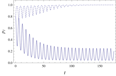
Now the morph $1$ globally dominates for $C=0$, i.e., for all initial conditions $\bar{p}_{1}$ goes to $1$ for large times; see Fig. 1. ($\bar{A}>0$ ensures that $p=0$ is unstable rest point, while $\bar{A}>\bar{B}$ ensures that $p=1$ is a stable rest point.) The global dominance does not change for $C<0$, because for a negative $C$ (and under conditions (40)), both new stable point $\pi_{1}$ and $\pi_{2}$ fall out of the interval $[0,1]$. One can call this dominating morph generalist stein , since it adapts to the time-averaged environment.

Figure 2:
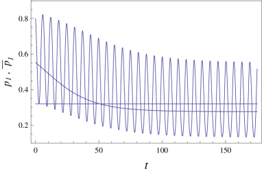
Oscillating curve: solution of (32) with $A(\omega t)=0.1-\sin(\omega t)$, $B(\omega t)=\cos(\omega t)$ with $\omega=1$ and the initial condition $p_{1}(0)=0.8$. With these $A(\tau)$ and $B(\tau)$, the parameter $C$ in (36) is equal to $0.5$.
Smooth curve: solution of the effective equation (37) with $\bar{A}=0.1$ and $\bar{B}=0$ and $C=0.5$, and initial condition $\bar{p}_{1}(0)=0.5528$. The difference between the initial conditions $\bar{p}_{1}(0)$ and $p_{1}(0)$ is calculated according to (25). With time $\bar{p}_{1}(t)$ converges to the rest point $\pi_{1}=0.276393$. For the unstable rest point we have $\pi_{2}=0.723607$.
Straight line: the long-time average of $p_{1}(t)$ equal to $0.32$. The approximate equality between the long-time average and $\pi_{1}$ improves upon increasing $C$ or decreasing $\bar{A}$ (and $|\bar{B}|$ if it is non-zero).

Provided that (40) holds, for

$$C\geq 2\bar{A}-\bar{B}+2\sqrt{\bar{A}^{\,2}-\bar{A}\bar{B}},$$ (41)

i.e., when $C$ is large enough, both $\pi_{1}$ and $\pi_{2}$ fall into the interval $[0,1]$, see Fig. 1, while if condition (41) does not hold, both $\pi_{1}$ and $\pi_{2}$ are not in this interval. When condition (41) saturates as equality, we get

$$\pi_{1}=\pi_{2}=\frac{1}{\bar{B}}\,\left[\,\bar{A}-\sqrt{\bar{A}^{\,2}-\bar{A}\bar{B}}\,\right],$$

which under conditions (40) is always in the interval $[0,1]$. Thus, when $C$ increases from a smaller value and then starts to satisfy (41), $\pi_{1}$ and $\pi_{2}$ move from the complex plane into the interval $[0,1]$, i.e., generically [from the viewpoint of conditions (40)] they do not appear in this interval via crossing its boundaries. This is natural, because at the boundaries the term $-C\bar{p}_{1}(1-\bar{p}_{1})$ in (37) nullifies.

Thus if condition (41) holds [in addition to (40)], a stable rest point $\pi_{1}$ emerges, which attracts all the trajectories that start from $\bar{p}_{1}(0)<\pi_{2}$: the polymorphism is created by the non-linear term $\propto C$ in (37).

Initial condition larger than the unstable rest point $\pi_{2}$, $\bar{p}_{1}(0)>\pi_{2}$, still tend to $\bar{p}_{1}=1$; see Fig. 1. Both stable rest points $\pi_{1}$ and $1$ are Evolutionary Stable States (ESS), meaning that they cannot be invaded by a sufficiently small mutant population hofbauer ; zeeman . The coexistence of two ESS one of which is interior (i.e., polymorphic) is impossible for a two-player replicator equation with constant pay-offs hofbauer ; zeeman , but it is possible for multi-player replicator equation broom_vick . We thus saw above an example of this behavior induced by time-varying environment.

Figure 3: Normal curve: $p_{1}(t)$ as obtained from solving (32) with $A(\omega t)=0.1-\sin(\omega t)$, $B(\omega t)=\cos(\omega t)$ with $\omega=1$, and initial condition $p_{1}(0)=0.5$; cf. Fig. 2.
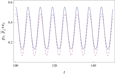
Dashed curve: $\bar{p}_{1}(t)+\epsilon_{1}(t)$, where $\bar{p}_{1}(t)$ is obtained from solving the effective equation (37), and where $\epsilon_{1}(t)=\epsilon_{1}[\bar{p}_{1}(t),\omega t]$ is the corresponding oscillating factor found in (16). According to (37), for considered times $\bar{p}_{1}$ converged to the stable fixed point $\pi_{1}$. For the present case $C=0.5$. The time-average of $p(t)$ does hold (37). Comparing with Fig. 4, where $\bar{A}$ is larger, it is seen that the approximate equality between $p_{1}(t)$ and $\bar{p}_{1}(t)+\epsilon_{1}(t)$ is better for the smaller value of $\bar{A}$.

Figure 4: The same as in Fig. 3, but with $A(\omega t)=0.121-\sin(\omega t)$, i.e. with a larger value of $\bar{A}$. The figure represents a metastable polymorphism, since $p(t)$ tends to increase slowly, i.e. it does not hold (37) for long times, and coverges to $p_{1}=1$ for times $t>230$.

V.3 Modification of the existing polymorphism

For $C=0$ and

$$\bar{B}>\bar{A}>0$$ (42)

there is a stable polymorphism at the rest point $\bar{p}_{1}={\bar{A}}/{\bar{B}}$. The presence of $C\not=0$ in (37) does not change this polymorphism qualitatively; only the value of the rest point shifts to $\pi_{1}$, which is now always in the interval $[0,1]$. The shift of the fixed point can be sizable.

Figure 5: As compared to Fig. (2) the value of $\bar{A}$ is decreased and is now equal to $0.05$. This changes the values of the rest points: $\pi_{1}=0.112702$ and $\pi_{2}=0.887298$. $p_{1}(t)$ and $\bar{p}_{1}(t)$ are still given by, respectively, oscillating curve and smooth curve. The value of the long-time average of $p_{1}(t)$ is now $0.1261$ (straight line), which is rather close to $\pi_{1}$ (the long-time limit of the smooth curve).

Likewise, for

$$\bar{B}<\bar{A}<0,$$ (43)

and $C=0$ there is an unstable polymorphism: all the initial conditions with $\bar{p}_{1}(0)<{\bar{A}}/{\bar{B}}$ end up at $p_{1}=0$ (morph 2 dominates), while those with $p_{1}(0)>{\bar{A}}/{\bar{B}}$ finish at $p_{1}=1$ (morph 1 dominates). Now $C\not=0$ in (37) shifts the unstable rest point to $\pi_{2}$. Again, the shift can be significant in some situations.

Conditions (40, 41, 42, 43) gave all possible non-trivial scenarios for two morphs, because other relations between $\bar{A}$ and $\bar{B}$ amount to interchanging the morphs.

V.4 Validity of the theory beyond the large-$\omega$ assumption

We now proceed to numerical comparison between the exact equation (32) and the effective (time-averaged) equation (37). Our aim is to show that the approximate validity of (37) extends beyond the large-$\omega$ limit.

Figs. 2, 3 and 4 compare the solution $p_{1}(t)$ of (32) with the corresponding solution $\bar{p}_{1}(t)$ of (37). Here we took $\omega=1$ to make clear that the frequency is not very large, and hence we are looking beyond the applicability of the above theory. The initial conditions $p_{1}(0)$ and $\bar{p}_{1}(0)$ were adjusted acording to (25). It is seen that though the qualitative agreement is good—in particular, $p_{1}(t)$ does converge with time to a polymorphic state, where its time-average is constant— there is a visible quantitative difference between the long-time averages calculated from the solution (32) and the rest point $\pi_{1}$ predicted from (37). The quantitative agreement is improved either by increasing $\omega$ (i.e., making the environmental oscillations faster) or by decreasing $\bar{A}$ and $\bar{B}$ (i.e., by slowing down the change of $p_{1}(t)$). This is demonstrated in Fig. 5.

As discussed in section III.2, the same initial conditions $p_{1}(0)$ can lead to a different attractor depending on the initial phase of the oscillating functions $A(\tau)$ and $B(\tau)$. This phenomenon is clearly seen on Fig. 6. We stress that this dependence is not a special feature of the considered stable polymorphic state. It will appear whenever there is a fast environment and the space of $p_{1}$ posseses several attractors, e.g., for the unstable polymorphic case studied in section V.3; see (43).

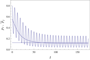
Fig. 7 shows that polymorphism survivies for a smaller frequency $\omega$.

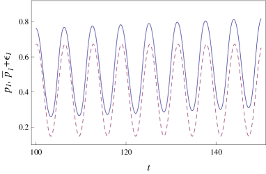
Fig. 4 demonstrates an interesting phenomenon of metastable polymorphism: the correspondence between (32) and (37)— i.e. between $p_{1}(t)$ and $\bar{p}_{1}+\epsilon_{1}$— is reasonable for times up $t\simeq 200$ (this characteristic time depends on initial conditions, the estimate seen in Fig. 4 was got with initial conditions $p_{1}(0)=0.5$). For larger times, the real solution converges to $p_{1}=1$. Thus $\bar{p}_{1}+\epsilon_{1}$ is capable of describing the metastable polymorphism within its life-time that is much longer than the characteristic time $1/\omega$ of environmental oscillations.

V.5 Two morphs within mathematical genetics

V.5.1 Interpretations in terms of genetics

Eq. (32) under additional condition

$$a_{12}(\tau)=a_{21}(\tau).$$ (44)

is a well-known Fisher equation from population genetics that describes the selection for a two-alelle gene (with frequencies $p_{1}$ and $p_{2}$, respectively) in one locus svi ; nagylaki_book . Then $a_{kl}$ are the Malthusian fitnesses for the zygote formed by the alleles $k$ and $l$. In particular, $a_{11}$ and $a_{22}$ refer to two homozygotes, while $a_{12}=a_{21}$ refers to the heterozygote. (A short and accessible review on genetic notions is given in Ref. svi .)

Let us now briefly comment on some of above results in the light of mathematical genetics, i.e. assuming (44). (1) Conditions (42) for a stable polymorphism translate to $\bar{a}_{12}>\bar{a}_{11},\,\bar{a}_{22}$, and refer to the heterozygote advantage svi .

(2) Note that $C$ in (36, 37) vanishes whenever the homozygotes are symmetric for all times ${a}_{11}(\tau)={a}_{22}(\tau)$, or whenever one allele (say allele 2) is recessive for all times ${a}_{11}(\tau)={a}_{12}(\tau)$. Both cases are easily solvable from (32) showing that the long-time behavior of $p_{1}$ is indeed governed by $\bar{A}$; so there is no room for the non-linear terms.

(3) The simplest case for non-zero $C$ is perhaps when the heterozygote fitness $a_{12}$ is constant in time, but the homozygote fitnesses $a_{11}(t)$ and $a_{22}(t)$ oscillate in time with different phases, e.g., when $a_{11}(t)$ is maximal $a_{22}(t)$ is minimal and vice versa.

(4) In section V.3, after (42) we stressed that the environmental influence, i.e. $C\not=0$, can sizably shift the stable rest-point thereby facilitating polymorphism. An important example of this type is given by the following mechanism of the recessive allele survival. For

$$\bar{B}=\bar{A}>0\quad{\rm or}\quad\bar{a}_{12}=\bar{a}_{11}>\bar{a}_{22},$$ (45)

the time-averaged fitnesses predict that the allele $2$ is recessive, i.e., its presence does not influence on the fitness of the heterozygote, while the fitness of the corresponding homozygote $22$ is smaller.

For $C<\bar{A}$ (in particular for $C=0$) the only stable rest point is $p_{1}=1$, which means that the allele is absent from the population. However, for $C>\bar{A}$ the poymorphism is recovered, since now [see (38)]

$$\pi_{1}=\bar{A}/C.$$ (46)

Thus the rapidly-changing environment can lead to a significant expression of the allele which is recessive in average.

V.5.2 Previous literature

Periodic time-dependencies in $A(t)$ and $B(t)$ [cf. (32)] were studied by Kimura kimura , Nagylaki nagylaki , and Li li in modelling environmental influences on genetic selection. These authors concentrate on cases (e.g. $A(t)=0$ or $B(t)=0$), where non-trivial mechanisms of polymorphism are absent. Below we shall focus on those situations, where Eq. (32) with time-independent $A$ and $B$ is not solvable exactly, but instead we obtain a non-trivial scenario of polymorphism.

Within the continuous-time consideration, Nagylaki nagylaki focussed on the case [cf. (23)]

$$A(\tau)=a\,h(\tau),\qquad B(\tau)=b\,h(\tau),\qquad\tau=\omega t$$ (47)

where $h(\tau)$ is a periodic function with $\overline{\,h(t)\,}=0$, and where $a$ and $b$ are constants. Note that $\bar{A}=\bar{B}=0$ according to (47). Now (32) can be solved exactly (i.e. independently from the magnitude of $\omega$), leading one to conclude that (32) cannot have stable rest-points, i.e. the convergence in time $p_{1}(t)\to p_{\rm rp}$ is excluded for $p_{\rm rp}\in[0,1]$. We are however interested in stable rest-points for the time-average $\bar{p}$, hence we turn to analyzing (37) under (47) and a sufficiently large $\omega$.

For this case we obtain from (37): $\dot{\bar{p}}_{1}=0$, a conclusion that is very well confirmed numerically and extends to higher orders in the $\frac{1}{\omega}$ expansion; see Appendix A and (93) there. Hence Nagylaki did not find polymorphism scenarios under conditions (47).

V.6 Average fitness and Lyapunov function

Eqs. (31) for the mean, time-averaged fitness $\Phi$ read after using (33, 34)

$$\Phi=2\bar{A}\bar{p}_{1}-\bar{B}\bar{p}_{1}^{2}.$$ (48)

Figure 6: This figure illustrates how the basins of attraction for two stable rest points $\pi_{1}$ and $1$ change depending on the phase of oscillating functions $A(\tau)$ [$\tau=\omega t$] and $B(\tau)$ at the initial time $t=0$.
Normal curve: solution of (32) with $A(\tau)=0.1-\sin(\omega t)$, $B(\tau)=\cos(\omega t)$ with $\omega=1$ and the initial condition $p_{1}(0)=0.8$.
Dashed curve: solution of (32) with $A(\tau)=0.1+\sin(\omega t)$, $B(\tau)=-\cos(\omega t)$ with $\omega=1$ and the same initial condition $p_{1}(0)=0.8$.
It is seen that for one phase $p_{1}(t)$ converges in averages to $\pi_{1}$, while for another phase it goes to $1$.

For $\bar{A}>0$ and $\bar{A}>\bar{B}$ (where the first morph dominates according to the average fitness), we get $\partial\Phi/\partial\bar{p}_{1}>0$. Hence $\Phi$ maximizes at $\bar{p}_{1}=1$, and this maximum is the only stable rest point of the replicator dynamics (37) with $C=0$. If however $C$ satisfies conditions (41), in the stable rest point $\bar{p}_{1}=\pi_{1}$ the mean fitness $\Phi$ is smaller than at the stable point $\bar{p}_{1}=1$. Moreover, for the initial conditions $\pi_{1}<\bar{p}_{1}(0)<\pi_{2}$, the mean fitness $\Phi$ decreases in the course of the relaxation to $\pi_{1}$. We confirmed this statement directly from equations of motion; see Table I.

Hence, the existence of a polymorphism does not have an adaptive value for the overall population, because the overall fitness decreases. We saw in section V.3 that the polymorphism which already exist on the level of the average environment appears to be robust with respect to environmental variations. So the value of polymorphism might be connected with this robustness.

Eq. (37) can be written as

$$\dot{\bar{p}}_{1} = \bar{p}(1-\bar{p})\,\frac{\partial\Psi}{\partial\bar{p}},$$ (49)

$$\Psi = 2\bar{A}\bar{p}_{1}-\bar{B}\bar{p}_{1}^{2}-C\bar{p}_{1}^{2}(1-\frac{2\bar{p}_{1}}{3})$$ (50)

$$= \Phi-C\bar{p}_{1}^{2}(1-\frac{2\bar{p}_{1}}{3}).$$

Hence $\Psi$ is increased by dynamics (37): $\dot{\Psi}\geq 0$. The difference between the mean fitness $\Phi$ and the Lyapunov function $\Psi$ is yet another indication that $\Phi$ does not need to increase in the slow time. Let us emphasize that there is no relation between the sign of $\Psi-\Phi$ and the existence of the environment-induced polymorphism.

Table 1: The solution of (32) was obtained under the same parameters as for Fig. 2. Then the time-dependence overall fitness $\Phi(t)$ was calculated accroding to $\Phi(t)=2A(\tau)p(t)-B(\tau)p^{2}(t)$; see (31, 33, 34) and note an irrelevant factor $a_{22}(t)$ in $\Phi(t)$ was neglected. After that we time-averaged this fitness around the points $t_{0}$ with the same time-window $t_{w}=25$: $\bar{\Phi}(t_{0})=\frac{1}{2t_{w}}\int_{t_{0}-t_{w}}^{t_{0}+t_{w}}{\rm d}s\,\Phi(s)$. The results for $\bar{\Phi}(t_{0})$ are displayed below and show that the time-averaged fitness decreases with increasing $t_{0}$.

$t_{0}=25$	$0.09627$
$t_{0}=75$	$0.07192$
$t_{0}=125$	$0.06467$
$t_{0}=175$	$0.06244$
$t_{0}=225$	$0.06167$

Figure 7: The purpose of this figure is to illustrate that the qualitative picture of polymorphism survives for smaller values of $\omega$, i.e., it survives for slower environment.
The same parameters as in Fig. 2, besides $\omega=0.25$.
Normal curve: solution of (32) with initial condition $p_{1}(0)=0.999$.
Dashed curve: solution of (32) with initial condition $p_{1}(0)=0.9999$.
It is seen that the stability domain of the rest point $p_{1}=1$ is heavily reduced.

VI The prisoner’s dilemma

As another pertinent illustration we consider the prisoner’s game shubik . There are two players $I$ and $II$. Each one has two strategies: $d$ (defect) and $c$ (cooperate). Pay-offs are determined by the following matrix

 d P,P T,S c S,T R,R= 1a11,a11a12,a212a21,a12a22,a22,fragments fragments dfragments P,Pfragments T,Sfragments cfragments S,Tfragments R,Rfragments 1fragmentsa11,a11fragmentsa12,a212fragmentsa21,a12fragmentsa22,a22\displaystyle\begin{tabular}[]{|c|c|c|}\hline\cr~{}${I}/{II}${}&$d$&$c$\\ \hline\cr~{}$d${}&~{}$P,\,P${}&~{}$T,\,S${}\\ \hline\cr\hline\cr~{}$c${}&~{}$S,\,T${}&~{}$R,\,R${}\\ \hline\cr\end{tabular}=\begin{tabular}[]{|c|c|c|}\hline\cr~{}${I}/{II}$&$1$&$2$\\ \hline\cr$1$&$a_{11},a_{11}$&$a_{12},a_{21}$\\ \hline\cr\hline\cr$2$&$a_{21},a_{12}$&$a_{22},a_{22}$\\ \hline\cr\end{tabular}\,,

 /III dc /III 12 /III dc /III 12 (57)

where e.g. the actions $d$ and $c$ by respectively $I$ and $II$ result to pay-offs $T$ and $S$, and where the second matrix in (57) relates to (1, 2). Eq. (57) becomes a dilemma after imposing:

$$T>R>P>S.$$ (58)

For both players defecting ($d$) is a dominant strategy, i.e. for both $I$ and $II$ acting $d$ yields a higher payoff than $c$ (cooperating), no matter what the opponent does; see (57, 58) and note that $(d,d)$ is the only Nash equilibrium of game (57). Both players can get $R>P$, if they both act $c$. But acting $c$ is vulnerable, since the opponent can change to $d$, gain out of this, and leave the cooperator with the minimal pay-off $S$. This makes the dilemma, which raised deep questions about rationality and cooperation shubik ; hofbauer ; peterson and produced a vast literature sandler ; dyson ; 15saakian ; weitz ; benica .

We focus on the case when pay-offs in (57) are time-periodic functions. Starting from (1, 2, 3), the time-dependent replicator equation reduces to (32), where

$$A(\tau)=T(\tau)-R(\tau),\qquad\tau=\omega t,$$ (59)

$$B(t)=T(\tau)-R(\tau)+S(\tau)-P(\tau).$$ (60)

If (58) is imposed on pay-offs at all times, then $A(\tau)>0$ and $A(\tau)>B(\tau)$. Then the always defection strategy $p_{1}=1$ is the only rest-point of the time-dependent (32), i.e. we are back to the prisoner’s dilemma.

A reasonable way to study the prisoner’s game for a rapidly changing environment is to impose condition (58) only on average

$$\bar{T}>\bar{R}>\bar{P}>\bar{S}.$$ (61)

Now (59–61) show that we are in the situation discussed in section V.2: there is no polymorphism on the level of the average fitness. But if condition (41) holds, the polymorphism does emerge. The positivity of $C=\frac{1}{\omega}\overline{\,(\hat{T}-\hat{R})(\widetilde{S}-\widetilde{P})\,}$ means here that the changes of $\widetilde{T}(\tau)-\widetilde{R}(\tau)$ and of $\widetilde{S}(\tau)-\widetilde{P}(\tau)$ are correlated.

Hence a time-dependent environment can resolve the prisoner’s dilemma that exists on the level of the average fitness. Other scenarios of resolving the dilemma are reviewed in tanimoto ; helbing ; devlin .

VII Three morphs

VII.1 Rock-scissors-paper game

Besides mathematical genetics nagylaki_book ; svi , the replicator dynamics is also applied for modeling biodiversity hofbauer ; zeeman . For concretness we shall focus on the situation with cyclic dominance, which exists for at least three morphs and requires asymmetric pay-offs. Cyclic dominance means that morphs $1$, $2$ and $3$ win over each other; e.g. $1$ beats $2$, $2$ beats $3$, and $3$ beats $1$ (rock-scissors-paper game) abraham . The simplest and perhaps most popular example of cyclic dominance is realized under the zero-sum condition in (2) [see (76) for an example]:

$$a_{kl}(\tau)=-a_{lk}(\tau),\qquad\tau=\omega t.$$ (62)

Eq. (62) means that the loss of the strategy $l$ is equal to the gain of $k$. Here is an incomplete list of realistic examples that contain cyclic dominance: i) mating strategies of side-blotched lizards sinervo ; ii) overgrowths by marine sessile organisms buss ; iii) competition between bacterial populations kerr .

Figure 8: The portrait of (63) for $\bar{a}_{12}=0.1$, $\bar{a}_{13}=0.1$, $\bar{a}_{23}=-0.1$, $\kappa_{1}=-0.65$ and $\kappa_{2}=0.65$; $\bar{p}_{1}$ and $\bar{p}_{2}$ are restricted by $0\leq\bar{p}_{1}\leq 1$, $0\leq\bar{p}_{2}\leq 1$, $\bar{p}_{1}+\bar{p}_{2}\leq 1$. Two rest points are denoted by square (saddle) and cycle (center). The closed orbits contain the center in their interior; orbits from the second class converge to $\bar{p}_{1}=1$. These two classes of orbits are separated by a dashed curve (separatrix), which is made by joining together two directions (stable and unstable) of the saddle. Arrows indicate direction of flow.

Though the zero-sum condition frequently does not produce structurally stable results , it is still very useful, since one can give a general description of the constant-payoff, $a_{kl}(\tau)=\bar{a}_{kl}$, zero-sum situation akin : starting from the interior of the simplex—that is starting from a point, where all the fractions are strictly positive: $p_{k}>0$—any trajectory either remains in the interior performing there a Hamiltonian motion , or it converges to the boundary, where some fractions $p_{k}$ are equal to zero. Once restricted to the boundary, the situation reduces to a zero-sum game with a smaller number of variables and the above reasoning can be applied again akin . Which scenario is realized depends on the concrete form of $a_{kl}(\tau)=\bar{a}_{kl}$; see below.

We stress that we also studied the three-morph case for the symmetric pay-off situation $a_{kl}(\tau)=a_{lk}(\tau)$, but the qualitative results on the environment-induced polymorphism were similar to the zero-sum case [see in this context section VIII below], so we choose to concentrate on the latter, because its presentation is simpler.

Under condition (62) the effective replicator equation (20, 21) reduces to

$$\dot{\bar{p}}_{i}={\sum}_{\alpha=1}^{3}\bar{p}_{i}\bar{a}_{i\alpha}\bar{p}_{\alpha}+\kappa_{i}\bar{p}_{1}\bar{p}_{2}\bar{p}_{3},\qquad i=1,2,3,$$ (63)

where

$$\kappa_{1}=b_{123}+b_{132}=\frac{1}{\omega}(-\overline{\widetilde{a}_{13}\,\hat{a}_{23}}+\overline{\widetilde{a}_{12}\,\hat{a}_{23}}),$$ (64)

$$\kappa_{2}=b_{213}+b_{231}=-\frac{1}{\omega}(\overline{\widetilde{a}_{23}\,\hat{a}_{13}}+\overline{\widetilde{a}_{12}\,\hat{a}_{13}}),$$ (65)

with

$$\kappa_{1}+\kappa_{2}+\kappa_{3}=0,$$ (66)

as needed for the conservation of normalization. It is seen that for the zero-sum situation the four-party terms $c_{klmn}$ disappear, since the payoffs are anti-symmetric.

Recall the interpretation of (63) with $i=1$: besides the payoffs $a_{12}$ and $a_{13}$ got by the strategy 1 when confronting with 2 and 3, respectively, there is a payment $\kappa_{1}$ which is received by the strategy 1 when it is confronted with the strategies $2$ and $3$ together. Eqs. (63) $i=2,3$ are interpreted in a similar way.

Figure 9: Parametric plot of solutions $p_{1}$ and $p_{2}$ of the replicator equation (1, 2) for $n=3$ (three morphs), $t\in[0,600]$ and $a_{12}(\omega t)=-a_{21}(\omega t)=0.1$, $a_{13}(\omega t)=-a_{31}(\omega t)=0.1+\sqrt{2\omega}\,a\sin(\omega t)$, $a_{23}(\omega t)=-a_{32}(\omega t)=0.1+\sqrt{2\omega}\,a\cos(\omega t)$, $a=\sqrt{0.65}$, $\omega=2$. The initial conditions are $p_{1}(0)=p_{2}(0)=0.25$.
Then the effective motion for $\bar{p}_{1}$ and $\bar{p}_{2}$ holds parameters shown on Fig. 8 independently on the value of $\omega$.

Figure 10: The first morph population $p_{1}$ versus time for the same parameters as in Fig. 9.
Black curve: $\omega=1.85$. Blue curve: $\omega=2$. Red curve: no environmental changes: $\omega=0$.
It is seen that $p_{1}(t)$ performs fast oscillations, and then slower motion that is oscillatory for the blue curve and increasing for the black curve.

The phase structure of (63) will be constructed in terms of independent variables $\bar{p}_{1}$ and $\bar{p}_{2}$ with $0\leq\bar{p}_{1}+\bar{p}_{2}\leq 1$. For the internal rest points we have:

$$\bar{a}_{12}\bar{p}_{2}+\bar{a}_{13}(1-\bar{p}_{1}-\bar{p}_{2})+\kappa_{1}\bar{p}_{2}(1-\bar{p}_{1}-\bar{p}_{2})=0,$$

$$- \bar{a}_{12}\bar{p}_{1}+\bar{a}_{23}(1-\bar{p}_{1}-\bar{p}_{2})+\kappa_{2}\bar{p}_{1}(1-\bar{p}_{1}-\bar{p}_{2})=0.$$ (67)

The Jacobian at these rest points is

$$-\left(\begin{array}[]{rr}\bar{p}_{1}(\bar{a}_{13}+\kappa_{1}\bar{p}_{2}){}{}{}&\frac{\bar{p}_{1}}{\bar{p}_{2}}(\bar{a}_{13}(1-p_{1})+\kappa_{1}\bar{p}_{2}^{2})\\ \\ \frac{\bar{p}_{2}}{\bar{p}_{1}}(\bar{a}_{23}(1-\bar{p}_{2})+\kappa_{2}\bar{p}_{1}^{2})&-\bar{p}_{1}(\bar{a}_{13}+\kappa_{1}\bar{p}_{2}){}{}{}\\ \end{array}\right),$$ (71)

while the eigenvalues of the Jacobian reads:

$$\pm\left[\,\bar{p}_{1}^{2}(\bar{a}_{13}+\kappa_{1}\bar{p}_{2})^{2}\right.$$

$$\left.+(\bar{a}_{13}(1-\bar{p}_{1})+\kappa_{1}\bar{p}_{2}^{2})(\bar{a}_{23}(1-\bar{p}_{2})+\kappa_{2}\bar{p}_{1}^{2})\right]^{1/2}.$$ (72)

Thus any interior rest point can be either saddle (two real eigenvalues of different sign) or center (two imaginary, complex conjugate eigenvalues).

We study in separate two different cases.

VII.2 Emergent polymorphism

One morph (say 1) dominates at the level of average pay-offs:

$$\bar{a}_{12}>0,\quad\bar{a}_{13}>0.$$ (73)

Eq. (63) with $i=1$ shows that the dominance is kept for $\kappa_{1}>0$. Hence for the existence of a polymorphism (due to $\kappa_{i}$ terms) it is necessary that 2 and 3 together win over 1 ($\kappa_{1}<0$), although in separate they loose to 1 according to (73).

There are two further necessary conditions for polymorphism that are deduced from the requirement that terms $\kappa_{i}\bar{p}_{1}\bar{p}_{2}\bar{p}_{3}$ do not turn to zero due to $p_{2}\to 0$ and/or $p_{3}\to 0$. Hence, as (63) shows, we should exclude the following two conditions:

$$\bar{a}_{23}<0\quad{\rm and}\quad\kappa_{2}<0,$$ (74)

$$\bar{a}_{23}>0\quad{\rm and}\quad\kappa_{3}=-\kappa_{1}-\kappa_{2}<0.$$ (75)

Then it is possible that the (non-linear) terms $\propto\kappa_{1}$, $\propto\kappa_{2}$ and $\propto\kappa_{3}$ in (63) change the phase-space portrait. Due to the non-linear terms two interior rest points appear in the triangle $0\leq\bar{p}_{1}\leq 1$, $0\leq\bar{p}_{2}\leq 1$, $\bar{p}_{1}+\bar{p}_{2}\leq 1$; see Fig. 8. The rest point with a smaller $\bar{p}_{1}$ is center, while the rest point with a larger $\bar{p}_{1}$ is a saddle.

The phase-space is thus divided into two domains: the first domains contains closed orbits around the center; see Fig. 8. These orbits correspond to the polymorphism: all the fractions $\bar{p}_{1}$, $\bar{p}_{2}$ and $\bar{p}_{3}$ stay non-zero for all times.

The second domain contains trajectories that converge to $\bar{p}_{1}=1$ for large times; see Fig. 8. The two domains are divided by the separatrix, a closed orbit that passes through the saddle; see Fig. 8. This scenario of polymorphism is similar to the one for the two-morph situation; see around (41).

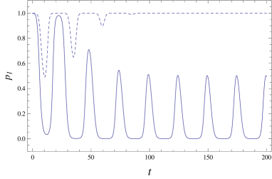
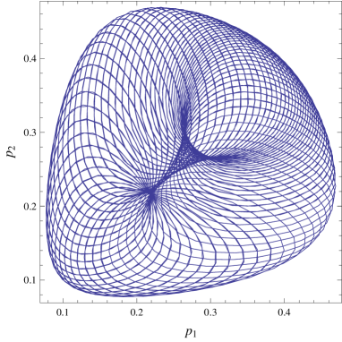
Figs. 9 and 10 show the behaviour of the original replicator equation (1, 2) with asymmetric pay-offs [cf. (62)], whose time-averages relate to (effective) parameters of Fig. 8. Now Fig. 9 shows that a single trajectory fills a sizable part of the phase-space available for the polymorphism. Fig. 10 contrasts the behavior of $p_{1}(t)$ in the polymorphic regime—which consists of fast and slow oscillations—with what we called a metastable polymorphism in Fig. 4; see the black curve in Fig. 10. Now the metastable polymorphism is realized when the frequency of environmental oscillations is not sufficiently large, i.e. $\omega=1.85$ versus $\omega=2$ for parameters of Figs. 9 and 10. It amounts to fast oscillations of $p_{1}(t)$ around a value sizably smaller than $1$, which then squeeze (for $t>100$), and then $p_{1}(t)$ goes to $1$, i.e. the polymorphism is destroyed, since the morph 1 eventually wins over $2$ and $3$; see the black curve on Fig. 10. Note that the life-time, $t\simeq 100$, of this metastable polymorphism is much larger than the period of environmental oscillations, as well as the relaxation time (to $p_{1}=1$) for the time-independent environment; see Fig. 10 and cf. Fig. 4.

VII.3 Existing polymorphism

Now let us assume that there is polymorphism already at the average level:

$$\bar{a}_{12}>0,\quad\bar{a}_{13}<0,\quad\bar{a}_{23}>0,$$ (76)

which means a cyclic competition: the strategy 1 wins over 2, but looses to 3, while 2 wins over $3$. This is the zero-sum version of the rock-scissors-paper game hofbauer ; zeeman .

Thus for $\kappa_{1}=\kappa_{2}=\kappa_{3}=0$ in (63) there is already one rest interior point, and the trajectories of the system are closed orbits around this rest point. It appears that after including the three-party ($\propto\kappa_{i}$) terms in (63) this rest point is simply shifted, and no new rest points appear for any size or magnitude of $\kappa_{i}$. We get the same conclusion as for the $n=2$ case: the non-linear (multi-party) terms do not spoil the polymorphism that already exists without them; see section V.3.

VIII Features of polymorphism related to Poincaré indices

In sections V and VII we noted that the non-linear terms (22) in the effective replicator equation produce either two new rest points (one stable and another unstable), or do not produce new rest points at all, although they can sizably shift the existing interior rest points (interior means that all components of the rest point are positive). Moreover, generically the new fixed points are produced directly in the interior, i.e., they do not have to appear via crossing of the boundaries for the simplex region $\{0\leq\bar{p}_{k}\leq 1\}_{k=1}^{n}$, $\sum_{k=1}^{n}\bar{p}_{k}=1$.

These effects suggest a common mechanism, which will be discussed below in terms of Poincaré indices. Recall that rest-points of the (non-linear) replicator dynamics (20, 21) are defined via $\Gamma_{k}[\pi]=0$. At regular rest points the Jacobian has non-zero determinant. We do not consider non-regular rest points, because they turn to be regular under small perturbation. Each regular rest point $\pi$ can be associated with its Poincaré index:

$${\rm Ind}[\pi]={\rm sign}\,\,{\rm det}\left.\left(\frac{\partial\Gamma_{i}[\bar{p}]}{\partial\bar{p}_{k}}\right)\right|_{\bar{p}=\pi},~{}~{}i,k=1,\ldots,n-1,$$

where $\frac{\partial\Gamma_{i}[\bar{p}]}{\partial\bar{p}_{k}}$ is the Jacobian matrix, and where we assume that in defining the Jacobian an independent set of coordinates was selected (since $\sum_{k=1}^{n}\bar{p}_{k}=1$, only $n-1$ probabilities $\bar{p}_{k}$ are independent). For instance in the two-dimensional situation (i.e., for two independent coordinates $\bar{p}_{1}$ and $\bar{p}_{2}$) the Poincaré of a saddle is $-1$ (because the Jacobian has two eigenvalues of different sign), while the Poincaré index of center is $+1$ (the Jacobian has two imaginary, complex conjugate eigenvalues). For a stable (unstable) rest-point in $p$-dimensional space the Poincaré index is equal to $(-1)^{p}$ ($1$).

Recall the content of the Poincaré-Hopf theorem as applied to the replicator equation hofbauer : for regular rest points $\pi$ of replicator dynamics (20, 21) one has

$${\sum}^{\prime}_{\pi}{\rm Ind}[\pi]=(-1)^{n-1},$$ (77)

where the sum ${\sum}^{\prime}_{\pi}$ is taken over those rest points $\pi$ of (20) which either have all their components strictly positive $\pi_{k}>0$, or if some of those components are zero, we have for each zero component $\pi_{i}=0$:

$$\left[{\cal F}_{i}(\bar{p})-{\sum}_{\alpha=1}^{n}\bar{p}_{\alpha}{\cal F}_{\alpha}(\bar{p})\left.\right]\right|_{\bar{p}=\pi}<0.$$ (78)

Condition (78) can be rephrased by saying that if a morph $i$ is missing within the rest-point (i.e. $\pi_{i}=0$), then its fitness is smaller than the mean fitness.

In addition to (77) we recall that the non-linear term $b_{klm}$ and $c_{klmn}$ in the effective replicator equation (20, 21) do not influence on the stability of the vertex rest points, where all $\bar{p}_{k}$’s besides one nullify; see our discussion in section III.3.

Eq. (77) shows that the conclusion of section V on the simultaneous emergence of two new rest-points (one stable and another unstable) is a general feature of (20, 21). Indeed, for even values of $n$, stable rest-points have ${\rm Ind}=-1$ (since the number of independent variables is odd, and each one brings factor $-1$ into the index). Hence according to (77), such a stable rest-point has to emerge simultaneously with another rest-point that has at least one unstable direction. Likewise, for odd values of $n$, where stable rest-points have ${\rm Ind}=1$.

Consider the three-morph situation with independent probabilities $\bar{p}_{1}$ and $\bar{p}_{2}$. If the non-linear terms (22) create a stable rest point in the interior (polymorphism), then the sum of Poincaré indices increases by $1$. So for (77) to hold, a saddle (with Poincaré index $-1$) rest-point has to be created as well. Taken together with the fact that the stability of the vertices is not altered, this then implies that two directions of the saddle has to joint together and form a closed curve that would separate the attraction basin of the newly created stable rest point. This was the scenario we saw in section VII .

Can the non-linear terms $b_{klm}$ and $c_{klmn}$ turn the stable polymorphic stable rest point—which exists already without them—into an unstable rest-point? This is not excluded by (77), because both rest-points have ${\rm Ind}=1$, but it is incompatible with the fact that the stability of the vertices is not altered by the non-linear terms. It is though not excluded that the non-linear terms would lead to changing of the old stable node into a unstable node surrounded by a stable limit cycle. Although we did not find such scenarios of the polymorphism emergence, from the conceptual viewpoint such a scenario will not change our basic qualitative conclusion that the poymorphism which exists without non-linear terms is (generically) not eliminated by them. The same argument shows that an unstable rest point cannot turn into a stable one without generating new rest points.

IX Summary and open problems

We discussed a mechanism of polymorphism that exists within continuous-time population dynamics due to a rapidly-changing (fine-grained) time-periodic environment. The characteristic time of environmental oscillations is larger than the the time over which the fractions of the sub-populations (morphs) change systematically (i.e. in average) levins ; clark . Various mechanisms of polymorpshim were at the focus of population biology for decades levins ; stein ; bull ; grant ; kassen_minireview ; wilke ; dempster ; janavar ; svi ; nagylaki_book . Such polymorphism scenarios as frequency-dependent selection and heterozygote advantage are at the basis of the current population thinking. Polymorphism induced by inhomogeneous environment also attracted muchattentionlevins ; stein ; bull ; grant ; kassen_minireview ; wilke ; dempster ; janavar ; svi ; nagylaki_book . So far this attention focussed on the slow (coarse-grained) environment, because early arguments implied that non-trivial polymorphism scenarios are absent for a rapidly-changing environment levins ; clark ; strobeck . Also the earlier studies of replicator dynamics in a time-dependent environment concentrated on those particular cases, where non-trivial scenarios of polymorphism are indeed absent nagylaki ; kimura ; li .

Starting from the replicator equation in a fast time-periodic environment we got an effective replicator equation for the time-averaged fractions of morphs. The main difference with the ordinary replicator equation in the time-independent environment—which for symmetric pay-offs reduces to the Fisher equations of mathematical genetics svi ; nagylaki_book —is that the fitness contains additional non-linear terms that appear due to the morphs tracking the environmental changes (the linear terms in the fitness correspond to the time-averaged environment). The presence of such tracking in a rapidly-changing (fine-grained) environment is established observationally drent . The form of non-linear terms allows to draw general conclusions on the stability and the effective fitness.

The non-linear terms can create a stable polymorphic state. But they generically do not destroy polymorphism that exists without the presence of these terms (i.e., for the averaged environment). Our results are worked out for three pertinent cases: genetic selection between two morphs (alleles), prisoner’s dilemma game (where polymorphism implies a resolution of the prisoner’s dilemma due to a time-varying environment), and the rock-paper-scissors game between three cyclically dominating morphs.

For the symmetric-pay-off situation [genetic selection] the fitness of the overall population can decrease due to the polymorphism. Once the existing polymorphism is generically not modified by the environment-induced terms, the adaptive value of the polymorphism is in increasing the structural stability of the population under influence of a time-dependent environment.

Several open problems are suggested by this research.

– One should clarify to which extent the uncovered mechanism of polymorphism is relevant for the phenomenon of sympatric speciation, where by contrast to the allopatric scenario the speciation is induced inside a single population doeb . (Within the allopatric scenario sub-populations are first isolated geographically and only then speciate). Interestingly, the decrease of the mean fitness was argued to be a prerequisite for the sympatric speciation doeb . Thus, our results hint at a sympatric speciation scenario due to a rapidly-changing, time-periodic environment.

– How to extend the present approach to multi-locus genetic selection, where polymorpshim related to a slow environment was studied recently in ppnass ?

– It will be interesting to develop the present approach for Eigen-Schuster model and its ramifications living on dynamic landscapes; see wilke for a review.

– The basic Lotka-Volterra equations of ecological dynamics can be recast in the form (2) and studied as replicators hofbauer . Note however that despite of this mathematical equivalence the ecological (and biological) content of Lotka-Volterra equations differs from that of replicators. This especially concerns the time-scale separation issues (i.e. the division between slow and fast), because Lotka-Volterra equations have additional time-scales svirizhev_logofet . Though the theory developed above does not apply directly to Lotka-Volterra equations, developing such applications is a pertinent avenue of future research.

– The present approach was developed assuming that all time-dependent selection coefficients have the same, well-defined period. This is restrictive an assumption, and we expect a richer dynamics upon relaxing it.

Acknowledgments

AEA and SGB were supported by SCS of Armenia, grants No. 18RF-002 and No. 18T-1C090. CKH was supported by Grant MOST 107-2112-M-259-006.

Appendix A Replicator equation under condition (23) with second-order terms

The purpose of this Appendix is to extend the asymptotic method of section III.1 to the order ${\cal O}(\omega^{-2})$, and thereby to understand implications of condition (23). Recall that under (23), the non-linear terms (22) in the fitness are absent. For simplicity we shall work with $n=2$ (two morphs).

Our first conclusion is that under condition (23) the terms ${\cal O}(\omega^{-2})$ that modify the replicator equation are perturbative—i.e. they have to be smaller than the terms given by the time-averages of pay-offs (selection coefficients). Our second conclusion (closely related to the first one) is that these terms are not useful for polymorphism.

Consider

$$\dot{p}=p(1-p)[A(\tau)-B(\tau)p],~{}~{}\tau=\omega t,~{}0\leq p(t)\leq 1,~{}$$ (79)

where $A(\tau)$ and $B(\tau)$ are rapidly-changing functions of time due to a large $\omega$. The time-averages, as well as the constant and oscillating parts of $A$ and $B$ are defined according to (3–7).

Following the method of section III, we look for the solution $p(t)$ of (79) as [cf. (8)]

$$p(t)=\bar{p}(t)+\frac{\epsilon_{1}[\bar{p}(t),\tau]}{\omega}+\frac{\epsilon_{2}[\bar{p}(t),\dot{\bar{p}}(t),\tau]}{\omega^{2}}+{\cal O}(\frac{1}{\omega^{3}}),$$ (80)

where the time-averages hold [cf. (9)]

$$\bar{\epsilon}_{1}=\bar{\epsilon}_{2}=0.$$ (81)

Putting (80) into (79) we get

$$\dot{\bar{p}}(t)+\frac{\dot{\bar{p}}(t)\epsilon_{1}^{\prime}}{\omega}+\frac{\dot{\bar{p}}(t)\epsilon_{2}^{\prime}}{\omega^{2}}+\partial_{\tau}\epsilon_{1}+\frac{1}{\omega}\partial_{\tau}\epsilon_{2}$$ (84)

$$=f[\bar{p},A(\tau),B(\tau)]+\frac{\epsilon_{1}}{\omega}f^{\prime}[\bar{p},A(\tau),B(\tau)]$$

$$+\frac{\epsilon_{2}}{\omega^{2}}f^{\prime}[\bar{p},A(\tau),B(\tau)]+\frac{\epsilon^{2}_{1}}{2\omega^{2}}f^{\prime\prime}[\bar{p},A(\tau),B(\tau)],$$

where we denoted

$$f(p,A,B)\equiv p(1-p)[A-Bp],$$ (85)

and $\epsilon^{\prime}$ and $f^{\prime}$ (resp. $\epsilon^{\prime\prime}$ and $f^{\prime\prime}$) means the first (resp. second) derivative over the first argument.

On the fast times we collect from (84) the orders of ${\cal O}(1)$ and ${\cal O}(1/\omega)$ respectively [cf. (15, 16)]:

$$\partial_{\tau}\epsilon_{1}=f[\bar{p},\widetilde{A},\widetilde{B}],$$ (86)

$$\partial_{\tau}\epsilon_{2}=-\dot{\bar{p}}\epsilon_{1}^{\prime}+\epsilon_{1}f[\bar{p},\widetilde{A},\widetilde{B}].$$ (87)

Before solving (86, 87), let us assume [cf. (23)]:

$$A(\tau)=\bar{A}+ah(\tau),\qquad A(\tau)=\bar{B}+bh(\tau),$$ (88)

where $h(\tau)=h(\tau+2\pi)$ is a periodic function of $\tau$, and where $\bar{A}$, $\bar{B}$, $a$ and $b$ are constants.

Then (86, 87) are solved as

$$\epsilon_{1} = f(\bar{p},a,b)\hat{h}(\tau),$$ (89)

$$\epsilon_{2} = [\,f(\bar{p},a,b)f^{\prime}(\bar{p},\bar{A},\bar{B})-\dot{\bar{p}}f^{\prime}(\bar{p},a,b)\,]\,\hat{\hat{h}}(\tau)$$ (90)

$$+\frac{1}{2}\,f(\bar{p},a,b)f^{\prime}(\bar{p},a,b)\left(\hat{h}^{2}(\tau)-\overline{\,\hat{h}^{2}\,}\,\right),$$

where ${\hat{h}}(\tau)$ and $\hat{\hat{h}}(\tau)$ are the first and second primitive of $h(t)$. Both hold the zero average condition $\overline{\,{\hat{h}}\,}=\overline{\,\hat{\hat{h}}\,}=0$.

Putting (89) and (90) into (84, 84) and taking the time-average, we get

$$\left(1-\chi\,[f^{\prime}(\bar{p},a,b)\,]^{2}\,\right)\dot{\bar{p}}=f(\bar{p},\bar{A},\bar{B})+\chi f(\bar{p},a,b)\times$$

$$\left[\frac{1}{2}f^{\prime\prime}(\bar{p},\bar{A},\bar{B})f(\bar{p},a,b)-f^{\prime}(\bar{p},\bar{A},\bar{B})f^{\prime}(\bar{p},a,b)\,\right],$$ (91)

$$\chi\equiv\overline{\,\hat{h}\,\hat{h}\,}/\omega^{2}.$$ (92)

In contrast to (20), where non-linear fitness terms need not be small, Eq. (91) shows that the non-linear fitness terms—those proportional to $\chi$—are smaller than the average fitness term $f(\bar{p},\bar{A},\bar{B})$. This is seen most clearly, when we put $\bar{A}=\bar{B}=0$ and notice that the right-hand-side of (92) disappears:

$$\left(1-\chi\,[f^{\prime}(\bar{p},a,b)\,]^{2}\,\right)\dot{\bar{p}}=\dot{\bar{p}}=0.$$ (93)

One can still ask whether the terms $\propto\chi$ can lead to polymorphism in the boundary situation, e.g. given $\bar{A}$ a positive but small (i.e. when $\bar{p}=0$ is marginally stable), can those terms change the stability of these boundary rest-point. The answer is negative.

References

- (1) R. Levins, Evolution in Changing Environments (Princeton University Press, 1968).
- (2) P.W. Hedrick, M.E. Ginevan and E.P. Ewing, Genetic Polymorphism in Heterogeneous Environments, Ann. Rev. Ecol. Syst. 7, 1 (1976). P.W. Hedrick, ibid, Genetic Polymorphism in Heterogeneous Environments: A Decade Later, 17, 535 (1986); ibid, Genetic Polymorphism in Heterogeneous Environments: The Age of Genomics, 37, 67-93 (2007).
- (3) L.A. Meyers and J.J. Bull, Fighting change with change: adaptive variation in an uncertain world, Tr. Ecol. Evol 17, 551-557 (2002).
- (4) V. Grant, Organismic Evolution (Freeman, SF, 1977).
- (5) R. Kassen, The experimental evolution of specialists, generalists, and the maintenance of diversity, J. Evol. Biol. 15, 173 (2002).
- (6) C.O. Wilke, C. Ronnewinkel, and T. Martinetz, Dynamic Fitness Landscapes in Molecular Evolution, Physics Reports, 349, 395-446 (2001).
- (7) E. Dempster, Maintenance of genetic heterogeneity, Cold Spring Harbor Symp. Quant. Biol. 20, 25 (1955).
- (8) J.B.S. Haldane and S.D. Jayakar, Polymorphism due to selection of varying direction, J. Genet. 58, 237 (1963). J.L. Cornette, Deterministic genetic models in varying environments, J. Math. Biol. 12, 173-186 (1981).
- (9) Yu.M. Svirezhev and V.P. Passekov, Findamentals of Mathematical Genetics (Dordrecht, Kluwer, 1990).
- (10) T. Nagylaki, Introduction to Theoretical Population Genetics (Springer-Verlag, Berlin, 1992).
- (11) T. Nagylaki, Polymorphisms in cyclically-varying environments, Heredity, 35, 67 (1975).
- (12) M. Kimura, Stochastic processes and distribution of gene sequences under natural selection, Cold Spring Harbor Symp. Quant. Biol., 20, 33 (1955).
- (13) W.-H. Li, Retention of cryptic genes in microbial populations, Mol. Biol. Evol., 1, 213-219 (1984).
- (14) J.H. Gillespie, The Causes of Molecular Evolution (Oxford Univ. Press, Oxford, 1991).
- (15) Lecture Notes on Biomathematics: Adaptation in Stochastic Environments, ed. J. Yoshimura and C.W. Clark (Springer-Verlag, Berlin, 1991).
- (16) C. Strobeck,Selection in a fine-grained environment, Am. Nat. 109, 419-425 (1975).
- (17) B.G. Miner and J.R. Vonesh, Effects of fine grain environmental variability on morphological plasticity, Ecol. Lett. 7, 794-801 (2004). N. M. Schoeppner and R. A. Relyea, Phenotypic plasticity in response to fine-grained environmental variation in predation, Functional Ecology, 23, 587 (2009).
- (18) A. Winn, Adaptation to fine-grained environmental variation: an analysis of within-individual leaf variation in an annual plant, Evolution 50, 1111 (1996).
- (19) J.-N. Jasmin and R. Kassen, On the experimental evolution of specialization and diversity in heterogeneous environments, Proc. R. Soc. B 274, 2761 (2007).
- (20) L.M. Cook, A two-stage model for Cepaea polymorphism, Phil. Trans. R. Soc. B 353, 1577 (1998).
- (21) I.A. Zakharov, Red and Black, Priroda, 5, 46 (1992). (In Russian)
- (22) M.E.N.Majerus and P.W.E. Kearns, Ladybirds (Slough, London, 1989).
- (23) L.A. Real, Fitness uncertainty and the role of diversification in evolution and behavior, Am. Nat. 115, 623-638 (1980). H. A. Orr, Evolution, Absolute fitness, relative fitness and utility, 61, 2997-3000 (2007).
- (24) E.B. Ford, Ecological genetics (Chapman and Hall, London, 1975)
- (25) T. Piersma and J. Drent, Phenotypic flexibility and the evolution of organismal design, Trends in Ecology and Evolution, 18, 228 (2003).
- (26) A. E. Allahverdyan and C.-K. Hu, Phys. Rev. Lett. 102, 058102 (2009).
- (27) J. Hofbauer and K. Sigmund, Evolutionary Games and Population Dynamics (Cambridge Univ. Press, 1998).
- (28) E.C. Zeeman, Population dynamics from game theory, in Z. Nitecki and C. Robinson (editors), Global Theory of Dynamical Systems (Lecture Notes in Mathematics, 819, Springer, Berlin). DOI: https://doi.org/10.1007/BFb0087009
- (29) R. Levins, Coexistence in a Variable Environment, The American Naturalist, 114, 765-783 (1979).
- (30) J.M. McNamara, Towards a richer evolutionary game theory, J. R. Soc. Interface, 10, 20130544 (2013).
- (31) J. W. Fox, The intermediate disturbance hypothesis should be abandoned, Trends in Ecology & Evolution, 28, 86-92 (2013).
- (32) D. Sheil and D.F. Burslem, Defining and defending Connell’s intermediate disturbance hypothesis: a response to Fox, Trends in Ecology & Evolution, 28, 571-572 (2013).
- (33) B. Thomas, Evolutionary stability: states and strategies, Theoretical Population Biology 26, 49 (1984).
- (34) L. D. Landau and E. M. Lifshitz, Mechanics (Pergamon Press, Oxford, 1976).
- (35) P. L. Kapitza, Dynamic stability of a pendulum with an oscillating point of suspension, Zh. Eksp. Teor. Fiz. 21, 588 (1951).
- (36) A. Ridinger and N. Davidson, Particle motion in rapidly oscillating potentials: The role of the potential’s initial phase, Phys. Rev. A 76, 013421 (2007).
- (37) F. Haake and M. Lewenstein, Adiabatic drag and initial slip in random processes, Phys. Rev. A 28, 3606 (1983). S. M. Cox and A. J. Roberts, Initial conditions for models of dynamical systems, Physica D 85, 126 (1995).
- (38) M. Broom, C. Cannings and G.T. Vickers, Bull. Math. Biol., Multi-player matrix games, 59, 931-952 (1997). L.A. Bach, T. Helvik and F.B. Christiansen, The evolution of n-player cooperation threshold games and ESS bifurcations, J. Theor. Biol. 238, 426-434 (2006).
- (39) M. Shubik, Game Theory, Behavior and the Paradox of the Prisoner’s Dilemma: Three Solutions, Journal of Conflict Resolution, 14, 181 (1970).
- (40) The Prisoner’s Dilemma, M. Peterson (ed.) (Cambridge University Press, Cambridge, 2015).
- (41) D. G. Arce and T. Sandler, The Dilemma of the Prisoners’ Dilemmas, KYKLOS 58, 3-24 (2005).
- (42) W. H. Press and F. J. Dyson, Iterated Prisoner’s Dilemma contains strategies that dominate any evolutionary opponent, Proc. Natl. Acad. Sci. U.S.A, 109, 10409 (2012).
- (43) T.Yakushkina, D. B. Saakian, A. Bratus, and C.-K. Hu, Evolutionary games with randomly changing payoff matrices, J. Phys. Soc. Japan 84, 064802 (2015).
- (44) E. Beninc , B. Ballantine, S.P. Ellner, and J. Huisman, Species fluctuations sustained by a cyclic succession at the edge of chaos, Proc. Natl. Acad. Sci. U.S.A, 112, 6389-6394 (2015).
- (45) J.S. Weitz et al., An oscillating tragedy of the commons in replicator dynamics with game-environment feedback, Proc. Natl. Acad. Sci. U.S.A., 113, E7518-E7525 (2016).
- (46) J. Tanimoto, Dilemma solving by the coevolution of networks and strategy in a game, Phys. Rev. E, 76, 021126 (2007).
- (47) D. Helbing and S. Lozano, Phase transitions to cooperation in the prisoner s dilemma, Phys. Rev. E, 81, 057102 (2010).
- (48) S. Devlin and T. Treloar, Network-based criterion for the success of cooperation in an evolutionary prisoner’s dilemma, Phys. Rev. E, 86, 026113 (2012).
- (49) M. Frean and E. R. Abraham, Rock-scissors-paper and the survival of the weakest, Proc. R. Soc. Lond. B 268, 1323-1327 (2001).
- (50) B. Sinervo and C. M. Lively, The rock-paper-scissors game and the evolution of alternative male strategies, Nature, 340, 240 (1996).
- (51) L. W. Buss, Competitive intransitivity and size-frequency distributions of interacting populations, Proc. Natl. Acad. Sci. U.S.A, 77, 5355 (1980).
- (52) B. C. Kirkup and M. A. Riley, Antibiotic-mediated antagonism leads to a bacterial game of rock-paper-scissors in vivo, Nature 428, 412 (2004). B. Kerr, M. A. Riley, M. W. Feldman, and B. J. M. Bohannan, Local dispersal promotes biodiversity in a real-life game of rock-paper-scissors, Nature, 418, 171 (2002).
- (53) G. Neumann and S. Schuster, Continuous model for the rock-scissors-paper game between bacteriocin producing bacteria, J. Math. Biol. 54, 815 (2007).
- (54) E. Akin and V. Losert, Evolutionary dynamics of zero-sum games, J. Math. Biology 20, 231 (1984).
- (55) M. Doebeli and U. Dieckmann, Evolutionary branching and sympatric speciation caused by different types of ecological interactions, Am. Nat. 156, S77 (2000); J. Evol. Biol. Adaptive dynamics as a mathematical tool for studying the ecology of speciation processes, 18, 1194-1200 (2005).
- (56) M. J. Wittmann, A. O. Bergland, M. W. Feldman, P. S. Schmidt, and D. A. Petrov, Seasonally fluctuating selection can maintain polymorphism at many loci via segregation lift, Proc. Natl. Acad. Sci. U.S.A, 114, E9932 E9941 (2017).
- (57) Yu.M. Svirizhev and D.O. Logofet, Stability of biological communities (Nauka, Moscow, 1978) (In Russian).