Scalar equilibrium problem and the limit distribution of the zeros of Hermite–Padé polynomials of type II

Abstract.

The existence of the limit distribution of the zeros of Hermite–Padé polynomials of type II for a pair of functions forming a Nikishin system is proved using the scalar equilibrium problem posed on the two-sheeted Riemann surface.

The relation of the results obtained here to some results of H. Stahl (1988) is discussed. Results of numerical experiments are presented. The results of the present paper and those obtained in the earlier paper of the second author [28], [32], [33] are shown to be in good accordance with both H. Stahl’s results and with results of numerical experiments.

Bibliography: [35] titles. 4 figures.

Keywords: Nikishin system, Hermite–Padé polynomials, equilibrium problem, potential theory, Riemann surfaces.

1. Introduction and statement of the problem

1.1.

The present paper continues the studies initiated by the second author in [28] and [33]. In these papers, a new scalar approach to the problem on the limit distribution of the zeros of Hermite–Padé polynomials for a pair of functions forming a Nikishin system was proposed and shown to be equivalent to the traditional vector approach (see [33], Theorem 1). We recall that the traditional approach to this problem is based on the solution of a vector equilibrium problem in potential theory with a $2\times 2$-matrix (known as the Nikishin matrix); see, first of all, [21], [22], [9], and [10], and also [1], [4], [17], and [18], and the references given therein. The vector equilibrium problem is known to have a unique solution given by vector measure $\vec{\lambda}=(\lambda_{1},\lambda_{2})$. Moreover, the limit distribution of the zeros of Hermite–Padé polynomials of type I exists and coincides with the measure $\lambda_{2}$, while for Hermite–Padé polynomials of type II the limit distribution of the zeros coincides with the measure $\lambda_{1}$. The alternative approach of [28] is that the equilibrium problem should be considered not on the Riemann sphere $\widehat{\mathbb{C}}$, but rather on some two-sheeted Riemann surface. As a result, the equilibrium problem becomes scalar, which leads to the appearance of another scalar equilibrium measure ${\boldsymbol{\lambda}}$, whose support now lies on the Riemann surface. In [28] it was shown that the limit distribution of the zeros of Hermite–Padé polynomials of type I coincides with the measure $\lambda=\pi_{2}({\boldsymbol{\lambda}})$, where $\pi_{2}$ is the canonical projection (a two-sheeted covering) of the Riemann surface under consideration to the Riemann sphere. In the present paper, the scalar equilibrium measure ${\boldsymbol{\lambda}}$ is used to characterize the limit distribution of the zeros of Hermite–Padé polynomials of type II for the same pair of functions $f_{1}$ and $f_{2}$ as in the papers [28] and [33] (see Section 1.2 below). As was already pointed out, on an example of two Markov functions $f_{1}$ and $f_{2}$ considered here (see formula (1.1) below) it was shown in [33] that these two approaches (the vector and scalar ones) are equivalent. The result on the limit distribution of the zeros of Hermite–Padé polynomials of type II (Theorem 2 below), which is obtained here in terms of the equilibrium measure ${\boldsymbol{\lambda}}$, was proved earlier by E. M. Nikishin [21] in a much more general setting using the traditional vector approach.

The idea of employing the potential theory on a Riemann surface for solving the problem on the limit distribution of the zeros of Hermite–Padé polynomials of multivalued analytic functions is generally not new. This approach was proposed earlier by H. Stahl in his two papers [26] and [27]. However, Stahl’s approach has not been further developed. The approach proposed by the second author in [28] is different from that of Stahl. In particular, as distinct from the second author’s papers [28] and [29], Stahl [26], [27] has never considered any extremal problem in potential theory or any equilibrium problem, even though he used potentials on a compact Riemann surface. Nevertheless, it turned out that for the pair of functions $f_{1}$ and $f_{2}$, which is considered both in [28] and in the present paper, these two methods give the same answer in the study of the so-called weak asymptotics of Hermite–Padé polynomials of both type I and type II. A relation between the results obtained by the authors’ and Stahl’s methods (the “third approach” in Stahl’s terms; see § 9 of [26]) is discussed below in § 3.

So, the ultimate purpose of the present paper is to further develop and apply the new scalar approach in the study of extremal and equilibrium problems that appear naturally when dealing with the limit behavior of the zeros of Hermite–Padé polynomials.

1.2.

As in [28] (see also [33]), we set

$$f_{1}(z):=\frac{1}{(z^{2}-1)^{1/2}},\quad f_{2}(z):=\frac{1}{\pi}\int_{-1}^{1}\frac{h(x)}{z-x}\frac{dx}{\sqrt{1-x^{2}}},\quad z\in D:=\widehat{\mathbb{C}}\setminus E,$$ (1.1)

where $E:=[-1,1]$ and we choose the branch of the function $(\,\cdot\,)^{1/2}$ such that $(z^{2}-1)^{1/2}/z\to 1$ as $z\to\infty$; for $x\in(-1,1)$ by $\sqrt{1-x^{2}}$ we mean the positive square root: $\sqrt{a^{2}}=a$ for $a\geqslant 0$. Here and everywhere in §§ 1 and 2 it is assumed that in (1.1) $h=\widehat{\sigma}$ is a Markov function supported in a regular compact set $F\subset\mathbb{R}\setminus E$; i.e.,

$$h(z)=\widehat{\sigma}(z):=\int_{F}\frac{d\sigma(t)}{z-t},\quad z\in\widehat{\mathbb{C}}\setminus F,$$ (1.2)

where $\sigma$ is a positive Borel measure with support $S(\sigma)$ in $F$ and such that $S(\sigma)=F$ and $\sigma^{\prime}(t):=d\sigma/dt>0$ almost everywhere (a.e.) on $F$ (see [28], [9], [10]). These conventions and notation will be kept throughout the paper. Moreover, we shall assume that the compact set $F$ consists of a finite number of closed intervals, $F=\bigsqcup_{j=1}^{p}F_{j}$, and the convex hull $\widehat{F}$ of $F$ has no common points with the closed interval $E$, $\widehat{F}\cap E=\varnothing$. For definiteness, we shall assume that the compact set $\widehat{F}$ lies on the real line to the right of $E$.

Since $f_{1}$ can be written as

$$f_{1}(z)=\frac{1}{\pi}\int_{-1}^{1}\frac{1}{z-x}\frac{dx}{\sqrt{1-x^{2}}},\quad z\in D,$$ (1.3)

from (1.1), (1.2), and (1.3) it follows that $\Delta f_{2}(x)/\Delta f_{1}(x)=\widehat{\sigma}(x)$, $x\in(-1,1)$, where $\Delta f_{j}(x)$ is the difference of the limit values (the jump) of the function $f_{j}$, $j=1,2$, in the upper and lower half-planes, respectively. It follows that the pair of functions $(f_{1},f_{2})$ forms a Nikishin system (for more on such systems, see [21], [22], and also [2], [4], [18], and the references given therein). Note that in the paper [31] an example of a multivalued analytic function $f$ is given such that the pair of functions $f,f^{2}$ forms a Nikishin system (under a minimal extension of the definition of a Nikishin system compared to the classical one). There exist classes of multivalued analytic functions $f$ such that the pair of functions $f,f^{2}$ can be naturally considered as a complex Nikishin system (see [24], [20], [29]). In connection with the new approach of [30] to the problem of efficient continuation of a given germ of a multivalued analytic function, this fact seems to be one of the main motivations for the study of equilibrium problems associated with complex Nikishin systems. Moreover, there are other applications of Hermite–Padé polynomials to the study of actual problems from various fields of theoretical and applied mathematics; see, for example, [19], [34], [16] and the references found there. It is the field of Nikishin systems which has received most attention in recent years. For example, much effort is now concentrated on the treatment of Hermite–Padé polynomials for Nikishin systems on star-like sets (see [17], [14], [15]). All this clearly shows the relevance of further development of the general theory of Hermite–Padé polynomials, and in the first instance, of Nikishin systems.

Given an arbitrary $n\in\mathbb{N}$, we let $\mathbb{P}_{n}$ denote the set of all polynomials of degree $\leqslant{n}$ with complex coefficients; $\mathbb{R}_{n}[\,\cdot\,]$ is the set of all polynomials with real coefficients and of degree $\leqslant{n}$ with respect to the corresponding variable. For an arbitrary polynomial $Q\in\mathbb{P}_{n}^{*}:=\mathbb{P}_{n}\setminus\{0\}$, by $\chi(Q)$ we denote the counting measure of the zeros of the polynomial $Q$ (counting multiplicities),

$$\chi(Q):=\sum_{\zeta:Q(\zeta)=0}\delta_{\zeta},$$

where $\delta_{\zeta}$ is the unit measure concentrated at a point $\zeta$ (the Dirac delta-function).

We now present some well-known facts about the limit distribution of the zeros of Hermite–Padé polynomials of type I and II for the pair of functions $f_{1},f_{2}$ forming a Nikishin system (see [22], [9], [10], [35], and also [18], [4], and the references quoted therein).

Given an arbitrary $n\in\mathbb{N}$, by $q_{2n}\in\mathbb{R}_{2n}[z]$, $q_{2n}\not\equiv 0$ and $p_{2n,1},p_{2n,2}\in\mathbb{R}_{2n-1}[z]$ we denote the Hermite–Padé polynomials of type II and index $n$ for a given pair of functions $f_{1},f_{2}$. Namely, these polynomials are defined (not uniquely) from the following two relations:

$$(q_{2n}f_{1}-p_{2n,1})(z)=O\left(\frac{1}{z^{n+1}}\right),\quad z\to\infty,$$ (1.4)

$$(q_{2n}f_{2}-p_{2n,2})(z)=O\left(\frac{1}{z^{n+1}}\right),\quad z\to\infty.$$ (1.5)

Let $M_{1}(E)$ be the class of all unit (positive Borel) measures with supports in $E$; let $M_{1}(F)$ be the analogous class of unit measures with supports in $F$. Next, let $g_{F}(z,\zeta)$ be the Green function for the domain $\Omega:=\overline{\mathbb{C}}\setminus{F}$ with logarithmic singularity at $z=\zeta$, let

$$G^{\mu}_{F}(z):=\int_{E}g_{F}(z,t)\,d\mu(t),\quad z\in D,$$ (1.6)

be the Green potential of the measure $\mu\in M_{1}(E)$, and let

$$U^{\mu}(z):=\int_{E}\log\frac{1}{|z-t|}\,d\mu(t),\quad z\in D,$$ (1.7)

be the logarithmic potential of the measure $\mu$. It is well known (see Chap. 5 of [22], and also [9], [10], [12]) that there exists a unique measure $\lambda_{E}\in M_{1}(E)$ such that $S(\lambda_{E})=E$ and

$$3U^{\lambda_{E}}(x)+G^{\lambda_{E}}_{F}(x)\equiv w_{E}=\operatorname{const}$$ (1.8)

on $E$ (the equilibrium relation). The measure $\lambda_{E}$ is known as the equilibrium measure with respect to the mixed Green-logarithmic potential $3U^{\mu}(x)+G^{\mu}_{F}(x)$, $w_{E}$ is the corresponding equilibrium constant.

The following result is well known (see [21], [22], [9], [10], [1]).

Theorem 1.

Let $f_{1},f_{2}$ be the pair of functions defined in (1.1), where $h(x)=\widehat{\sigma}(x)$, $S(\sigma)=F$ and $\sigma^{\prime}(t)=d\sigma/dt>0$ a.e. on $F$. Given an arbitrary $n\in\mathbb{N}$, let $q_{2n}$ be the Hermite–Padé polynomials of type II defined by (1.4)–(1.5). Then $\operatorname{deg}{q_{2n}}=2n$ for each $n$, the polynomial $q_{2n}$ is defined uniquely by the normalization $q_{2n}(z)=z^{2n}+\dotsb$, all the zeros of the polynomial $q_{2n}$ are simple and lie in the interval $(-1,1)$, and moreover,

$$\frac{1}{n}\chi(q_{2n})\overset{*}{\longrightarrow}2\lambda_{E}$$ (1.9)

as $n\to\infty$, where $\lambda_{E}\in M_{1}(E)$ is the equilibrium measure for problem (1.8).

In (1.9) and in what follows, by the convergence “$\overset{*}{\longrightarrow}$” we mean the weak^∗ convergence in the space of measures $M_{1}(E)$.

Note that the above result on the limit distribution of the zeros of Hermite–Padé polynomials of type II is a very particular case of a more general result proved in a more general setting than that considered in Theorem 1 (see, first of all [21], [22], Ch. 5, § 7, Theorem 7.1, and also [9], [1]). All these results have been obtained in the framework of the traditional vector approach to the problem on the limit distribution of the zeros of Hermite–Padé polynomials, the foundations of which was laid by A. A. Gonchar and E. A. Rakhmanov in 1981 (see [7]).

The purpose of the present paper is to prove, using the new approach proposed in the series of papers [28], [33] and residing in the scalar equilibrium problem on a Riemann surface, that under the hypotheses of Theorem 1 there exists the limit distribution of the Hermite–Padé polynomials $q_{2n}$ of type II without having recourse to the vector equilibrium problem, but rather employing directly the terms related to the scalar equilibrium problem.

1.3.

We shall require the following notation and definitions from [28].

Given $z\in D=\widehat{\mathbb{C}}\setminus E$, we set

$$\varphi(z):=z+(z^{2}-1)^{1/2};$$ (1.10)

this is the inverse of the Joukowsky function (we recall that everywhere in the present paper we choose the branch of the function $(\cdot)^{1/2}$ such that $(z^{2}-1)^{1/2}/z\to 1$ as $z\to\infty$). The function $\varphi$ is single-valued meromorphic in the domain $D$.

Let $\mathfrak{R}_{2}=\mathfrak{R}_{2}(w)$ be the Riemann surface of the function $w^{2}=z^{2}-1$, $w(z)=\pm(z^{2}-1)^{1/2}$, $z\in D$. We shall assume that a point $\mathbf{z}\in\mathfrak{R}_{2}$ has the form $\mathbf{z}=(z,w)$. Let $\pi_{2}\colon\mathfrak{R}_{2}\to\widehat{\mathbb{C}}$ be the two-sheeted covering of the Riemann sphere $\widehat{\mathbb{C}}$ ($\pi_{2}$ is the canonical projection): $\pi_{2}(\mathbf{z})=z$. From the equality $\varphi(\mathbf{z})=z+w$ one can define the function $\varphi$ on the Riemann surface $\mathfrak{R}_{2}$. More precisely, we set $\Phi(\mathbf{z})=z+w$. The function $\Phi(\mathbf{z})$ thus defined is the natural analytic extension of the function $\varphi(z)$ from the domain $D\subset\widehat{\mathbb{C}}$ to the entire Riemann surface $\mathfrak{R}_{2}$.

Let us now define the global partition of the Riemann surface $\mathfrak{R}_{2}$ into open sheets $\mathfrak{R}_{2}^{(0)}$ (the zero sheet) and $\mathfrak{R}_{2}^{(1)}$ (the first sheet) by the rule: $z^{(0)}:=(z,(z^{2}-1)^{1/2})\in\mathfrak{R}_{2}^{(0)}$, $z^{(1)}:=(z,-(z^{2}-1)^{1/2})\in\mathfrak{R}_{2}^{(1)}$, $z\in D$. As usual, the zero sheet $\mathfrak{R}_{2}^{(0)}$ of the Riemann surface $\mathfrak{R}_{2}$ is identified with the “physical” domain $D=\widehat{\mathbb{C}}\setminus E$ on the Riemann sphere. We set $g_{2}(\mathbf{z}):=-\log|\Phi(\mathbf{z})|=\log|z-w|$. From the above partition of the Riemann surface $\mathfrak{R}_{2}$ into sheets, we have $\Phi(z^{(0)})=\varphi(z)$, $\Phi(z^{(1)})=1/\varphi(z)$. Hence $g_{2}(z^{(0)})=-\log|z|+O(1)$, $g_{2}(z^{(1)})=\log|z|+O(1)$, $z\to\infty$, and $g_{2}(z^{(0)})<g_{2}(z^{(1)})$. The above partition of the Riemann surface $\mathfrak{R}_{2}$ into sheets is a Nuttall partition (see [23], § 3, [13], Lemma 5). Moreover, $\pi_{2}(\mathfrak{R}_{2}^{(0)})=\pi_{2}(\mathfrak{R}_{2}^{(1)})=D$.

We set $V(\mathbf{z}):=-\log|\Phi(\mathbf{z})|=\log|z-w|$ for $\mathbf{z}\in\mathfrak{R}_{2}$; in what follows, the function $V(\mathbf{z})$ will play the role of an external field in the equilibrium problem considered here. Let $\mathbf{F}=F^{(1)}\subset\mathfrak{R}_{2}$ be the compact set lying on the first sheet $\mathfrak{R}^{(1)}_{2}$ of the Riemann surface $\mathfrak{R}_{2}$ and such that $\pi_{2}(\mathbf{F})=F$.

By $M_{1}(\mathbf{F})$ we denote the space of all unit (positive Borel) measures with support in $\mathbf{F}$. Following [28] and [33], for an arbitrary measure ${\boldsymbol{\mu}}\in M_{1}(\mathbf{F})$, we introduce the function $P^{{\boldsymbol{\mu}}}(\mathbf{z})$ of a point $\mathbf{z}\in\mathfrak{R}_{2}$ (the “potential” of the measure ${\boldsymbol{\mu}}$, see Remark 2 in [33]),

$$P^{{\boldsymbol{\mu}}}(\mathbf{z}):=\int_{\mathbf{F}}\log\frac{\left|1-1/\bigl{(}\Phi(\mathbf{z})\Phi(\mathbf{t})\bigr{)}\right|}{|z-t|^{2}}\,d{\boldsymbol{\mu}}(\mathbf{t}),\quad\mathbf{z}\in\mathfrak{R}_{2}\setminus(F^{(0)}\cup F^{(1)}),$$ (1.11)

and consider the corresponding energy of the measure ${\boldsymbol{\mu}}$ (cf. [5] and [6])

$$J({\boldsymbol{\mu}}):=\iint_{\mathbf{F}\times\mathbf{F}}\log\frac{\left|1-1/\bigl{(}\Phi(\mathbf{z})\Phi(\mathbf{t})\bigr{)}\right|}{|z-t|^{2}}\,d{\boldsymbol{\mu}}(\mathbf{z})\,d{\boldsymbol{\mu}}(\mathbf{t})=\int_{\mathbf{F}}P^{\boldsymbol{\mu}}(\mathbf{z})\,d{\boldsymbol{\mu}}(\mathbf{z})$$ (1.12)

with respect to the kernel

$$\log\frac{\left|1-1/\bigl{(}\Phi(\mathbf{z})\Phi(\mathbf{t})\bigr{)}\right|}{|z-t|^{2}}.$$

We also define the energy of the measure ${\boldsymbol{\mu}}$ in an external field $V$,

$$J_{V}({\boldsymbol{\mu}}): =\iint_{\mathbf{F}\times\mathbf{F}}\biggl{\{}\log\frac{\left|1-1/\bigl{(}\Phi(\mathbf{z})\Phi(\mathbf{t})\bigr{)}\right|}{|z-t|^{2}}+V(\mathbf{z})+V(\mathbf{t})\biggr{\}}\,d{\boldsymbol{\mu}}(\mathbf{z})\,d{\boldsymbol{\mu}}(\mathbf{t})$$

$$=\int_{\mathbf{F}}P^{\boldsymbol{\mu}}(\mathbf{z})\,d{\boldsymbol{\mu}}(\mathbf{z})+2\int_{\mathbf{F}}V(\mathbf{z})\,d{\boldsymbol{\mu}}(\mathbf{z}).$$ (1.13)

By $M_{1}^{\circ}(\mathbf{F})$ we denote the set of all measures ${\boldsymbol{\mu}}\in M_{1}(\mathbf{F})$ with finite energy $J_{V}({\boldsymbol{\mu}})$. In what follows, we shall identify the measure ${\boldsymbol{\mu}}\in M_{1}(\mathbf{F})$ with the measure $\mu=\pi_{2}({\boldsymbol{\mu}})\in M_{1}(F)$, where $\pi_{2}({\boldsymbol{\mu}})(e):={\boldsymbol{\mu}}(e^{(1)})$ for any ${\boldsymbol{\mu}}$-measurable set $e\subset F$.

The following result combines the principal results of the papers [28] and [33].

Proposition 1 ((see [28], Theorem 1; [33], Theorem 1 and Remark 3)).

In the class $M_{1}^{\circ}(\mathbf{F})$, there exists a unique (scalar) measure ${\boldsymbol{\lambda}}=\lambda_{\mathbf{F}}\in M_{1}^{\circ}(\mathbf{F})$ with the following property:

$$J_{V}({\boldsymbol{\lambda}})=\inf_{{\boldsymbol{\mu}}\in M_{1}(\mathbf{F})}J_{V}({\boldsymbol{\mu}}).$$ (1.14)

The measure ${\boldsymbol{\lambda}}$ is completely characterized by the following equilibrium condition:

$$P^{\boldsymbol{\lambda}}(\mathbf{z})+V(\mathbf{z})\equiv w_{\mathbf{F}},\quad\mathbf{z}\in\mathbf{F}=S({\boldsymbol{\lambda}}).$$ (1.15)

1.4.

In the present paper we employ the scalar equilibrium problem (1.15) to prove the following

Theorem 2.

Let $f_{1}$ and $f_{2}$ be the functions defined by relations (1.1) and let $q_{2n}$, $n\in\mathbb{N}$, be the monic Hermite–Padé polynomials of type II defined by the two relations (1.4)–(1.5). Then $\operatorname{deg}{q_{2n}}=2n$ for all sufficiently large $n$, all the zeros of the polynomial $q_{2n}$ lie in the interval $(-1,1)$, and moreover,

$$\lim_{n\to\infty}\log\frac{1}{|q_{2n}(z)|^{1/n}}=U^{\lambda_{F}}(z)-\int_{F}\log\frac{1}{|\varphi(z)-\varphi(t)|}\,d\lambda_{F}(t)-2\log|\varphi(z)|+\log{2},\\ z\in\mathbb{C}\setminus{E},$$ (1.16)

uniformly inside the domain $\mathbb{C}\setminus{E}$, where $q_{2n}(z)=z^{2n}+\dotsb$, $\lambda_{F}=\pi_{2}(\lambda_{\mathbf{F}})$, $\lambda_{\mathbf{F}}$ is the equilibrium measure for problem (1.15).

The following corollary can be obtained from Lemma 2 (see § 4 below) and the fact that $\log|\varphi(z)|=g_{E}(z,\infty)=\gamma_{E}-U^{\tau_{E}}(z)$, where $g_{E}(z,\infty)$ is the Green function for the domain $D$, $\tau_{E}$ is the Chebyshev measure for the interval $E$, and $\gamma_{E}=\log 2$ is the Robin constant for $E$.

Corollary 1.

Under the hypotheses of Theorem 2,

$$\frac{1}{n}\chi(q_{2n})\overset{*}{\longrightarrow}2\mu,\quad n\to\infty,$$ (1.17)

where

$$\mu=\frac{1}{4}\beta_{E}(\lambda_{F})+\frac{3}{4}\tau_{E}.$$ (1.18)

Indeed, representation (1.18) for the measure $\mu$ is obtained by applying the operator $\mathrm{dd}^{c}$ to the right-hand side of (1.16) and using Lemma 2.

According to Theorem 1 of [33], the right-hand side of (1.18) is equal to $\lambda_{1}=\lambda_{E}$ (see Theorem 1 above). Thus, relation (1.17) is equivalent to (1.9).

2. Proof of Theorem 2

2.1.

Let $q_{2n}$ be the Hermite–Padé polynomials of type II defined by (1.4)–(1.5). Let $\gamma_{1}$ be a closed contour separating the closed interval $E$ from the compact set $F$ and the point at infinity $z=\infty$. From (1.4) it follows that the following orthogonality relations hold:

$$\int_{\gamma_{1}}q_{2n}(\zeta)\zeta^{k}f_{1}(\zeta)\,d\zeta=0,\quad k=0,\dots,n-1.$$ (2.1)

Therefore, for any Chebyshev polynomial (of the first kind) $T_{k}(\zeta)=\varphi^{k}(\zeta)+\varphi^{-k}(\zeta)=2^{k}\zeta^{k}+\dotsb$, $k=0,\dots,n-1$, we have

$$\int_{\gamma_{1}}q_{2n}(\zeta)T_{k}(\zeta)f_{1}(\zeta)\,d\zeta=0.$$ (2.2)

Since $\Delta f_{1}(x)=-2i/\sqrt{1-x^{2}}$ for $x\in(-1,1)$, we get from (2.2) that

$$\int_{-1}^{1}q_{2n}(x)T_{k}(x)\,\frac{dx}{\sqrt{1-x^{2}}}=0,\quad k=0,\dots,n-1.$$ (2.3)

Therefore, we have the representation

$$q_{2n}(x)=\sum_{j=n}^{2n}c_{j}T_{j}(x);$$ (2.4)

here $c_{j}\in\mathbb{R}$, because $q_{2n}$ is a real polynomial. Now an appeal to (1.5) shows that

$$\int_{\gamma_{1}}q_{2n}(\zeta)p(\zeta)f_{2}(\zeta)\,d\zeta=0,$$ (2.5)

where $p\in\mathbb{P}_{n-1}$ is an arbitrary polynomial. Using representation (2.4) for the polynomial $q_{2n}$, we have from (2.5)

$$\int_{\gamma_{1}}\biggl{\{}\sum_{j=n}^{2n}c_{j}T_{j}(\zeta)\biggr{\}}p(\zeta)f_{2}(\zeta)\,d\zeta=0,$$ (2.6)

or, equivalently,

$$\int_{-1}^{1}\biggl{\{}\sum_{j=n}^{2n}c_{j}T_{j}(x)\biggr{\}}p(x)\Delta f_{2}(x)\,dx=0.$$

Hence, using representation (1.1) for the function $f_{2}(x)$, we have, for any polynomial $p\in\mathbb{P}_{n-1}$,

$$\int_{-1}^{1}\biggl{\{}\sum_{j=n}^{2n}c_{j}T_{j}(x)\biggr{\}}p(x)\widehat{\sigma}(x)\,\frac{dx}{\sqrt{1-x^{2}}}=0.$$ (2.7)

Given $z\in D$, let

$$H_{n}(z):=\frac{1}{\pi}\int_{-1}^{1}\frac{T_{n}(x)}{z-x}\frac{dx}{\sqrt{1-x^{2}}}=\frac{1}{\pi T_{n}(z)}\int_{-1}^{1}\frac{T^{2}_{n}(x)}{z-x}\frac{dx}{\sqrt{1-x^{2}}},\quad n=0,1,\dots,$$ (2.8)

be the functions of the second kind corresponding to the Chebyshev polynomials $T_{n}$. It is well known that the Chebyshev polynomials $T_{n}(z)=2^{n}z^{n}+\dotsb$ satisfy the following recursion relation:

$$y_{n}=2zy_{n-1}-y_{n-2},\quad n=1,2,\dots,\quad\text{where}\quad y_{-1}=0,\ \ y_{0}=1.$$ (2.9)

From (2.8) it follows that this relation is also satisfied by the functions of the second kind $H_{n}$ (but with different initial conditions: $H_{-1}(z)\equiv 1$, $H_{0}(z)=f_{1}(z)=1/(z^{2}-1)^{1/2}$). Moreover, using (2.8) we find that, for $x\in(-1,1)$,

$$\Delta H_{n}(x):=H_{n}(x+i0)-H_{n}(x-i0)=T_{n}(x)\frac{2}{i\sqrt{1-x^{2}}}.$$ (2.10)

From (2.10) it easily follows that relation (2.7) is equivalent to the relation

$$\int_{\gamma_{1}}\biggl{\{}\sum_{j=n}^{2n}c_{j}H_{j}(\zeta)\biggr{\}}p(\zeta)\widehat{\sigma}(\zeta)\,d\zeta=0,$$ (2.11)

where $\gamma_{1}$ is an arbitrary contour separating the closed interval $E$ from the point at infinity and the compact set $F$, besides, $p\in\mathbb{P}_{n-1}$ is a polynomial, and (see (1.2)),

$$\widehat{\sigma}(z)=\int_{F}\frac{d\sigma(t)}{z-t},\quad z\notin F.$$

By the second equality in (2.8),

$$H_{j}(z)=O\left(\frac{1}{z^{j+1}}\right),\quad z\to\infty,$$

and hence (2.11) can be transformed to read

$$\int_{\gamma_{2}}\biggl{\{}\sum_{j=n}^{2n}c_{j}H_{j}(\zeta)\biggr{\}}p(\zeta)\widehat{\sigma}(\zeta)\,d\zeta=0,$$

where $\gamma_{2}$ is an arbitrary closed contour separating the compact set $F$ from the closed interval $E$ and the point at infinity. From the last relation we find that

$$\int_{F}\biggl{\{}\sum_{j=n}^{2n}c_{j}H_{j}(t)\biggr{\}}p(t)\,d\sigma(t)=0$$ (2.12)

for an arbitrary polynomial $p\in\mathbb{P}_{n-1}$ and some real numbers $c_{j}$, $j=n,\dots,2n$.

Now, assume for definiteness that $n=2m-1$ is an odd number (the case of even $n=2m$ is dealt with similarly). From the recursion relation (2.9) it easily follows that

$$\sum_{j=n}^{2n}c_{j}H_{j}(z)=q_{n,1}(z)H_{n+m-1}(z)+q_{n,2}(z)H_{n+m}(z),$$ (2.13)

and

$$q_{2n}(z)=\sum_{j=n}^{2n}c_{j}T_{j}(z)=q_{n,1}(z)T_{n+m-1}(z)+q_{n,2}(z)T_{n+m}(z)$$ (2.14)

(cf. [14], Proposition 2.12, Lemma 5.1, and [15]), where the polynomials $q_{n,1},q_{n,2}$ lie in $\mathbb{R}_{m-1}[z]$ (we recall that $n=2m-1$). It is worth pointing out that in (2.13) and (2.14) the polynomials $q_{n,1}$ and $q_{n,2}$ are the same.

So, relation (2.12) assumes the form

$$\int_{F}\bigl{\{}q_{n,1}(t)H_{n+m-1}(t)+q_{n,2}(t)H_{n+m}(t)\bigr{\}}p(t)\,d\sigma(t)=0$$ (2.15)

for an arbitrary polynomial $p\in\mathbb{R}_{n-1}[t]$. Using (2.13), the equality $\varphi^{\prime}(z)/\varphi(z)=1/(z^{2}-1)^{1/2}$, and the well known fact that for the Chebyshev polynomials the corresponding functions of the second kind read as

$$H_{n}(z)=\frac{\varkappa_{n}\varphi^{\prime}(z)}{\varphi^{n+1}(z)}=\frac{\varkappa_{n}}{\varphi^{n}(z)(z^{2}-1)^{1/2}},$$ (2.16)

where the constant $\varkappa_{n}\neq 0$, the orthogonality relation (2.15) assumes the form

$$\int_{F}\biggl{\{}q_{n,1}(t)+\frac{q_{n,2}(t)}{\varphi(t)}\biggr{\}}\frac{\varphi^{\prime}(t)}{\varphi^{n+m}(t)}p(t)\,d\sigma(t)=0.$$ (2.17)

2.2.

We now introduce the function

$$g_{n}(\mathbf{z}):=q_{n,1}(z)+q_{n,2}(z)\Phi(\mathbf{z}),\quad\mathbf{z}\in\mathfrak{R}_{2},$$

and rewrite relation (2.17) in the form

$$\int_{F^{(1)}}g_{n}(t^{(1)})\Phi(t^{(1)})^{n+m}\varphi^{\prime}(t)p(t)\,d\sigma(t)=0$$ (2.18)

or, equivalently,

$$\int_{F^{(1)}}g_{n}(t^{(1)})\Phi(t^{(1)})^{n+m-1}\frac{p(t)}{w(t^{(1)})}\,d\sigma(t)=0.$$ (2.19)

The function $g(\mathbf{z})$ is meromorphic on the Riemann surface $\mathfrak{R}_{2}$ defined above. Recall that in view of the above partition of the Riemann surface $\mathfrak{R}_{2}$ into sheets, we have $\Phi(z^{(0)})=\varphi(z)$, $\Phi(z^{(1)})=1/\varphi(z)$. Since the polynomials $q_{n,1},q_{n,2}$ lie in $\mathbb{P}_{m-1}$, the function $g_{n}(\mathbf{z})$ has a pole of order $\ell_{0}\leqslant m$ at the point $\mathbf{z}=\infty^{(0)}$ and has a pole of order $\ell_{1}\leqslant m-1$ at the point $\mathbf{z}=\infty^{(1)}$. The function $g_{n}(\mathbf{z})$ has no other poles on the Riemann surface $\mathfrak{R}_{2}$. From Abel’s theorem it follows that the function $g_{n}(\mathbf{z})$ has $\ell_{0}+\ell_{1}=\ell_{2}\leqslant 2m-1=n$ “free” (depending on $n$) zeros at some points $\mathbf{b}_{1,n},\dots,\mathbf{b}_{n,\ell_{2}}$ on the Riemann surface $\mathfrak{R}_{2}$.

Since the polynomials $q_{n,1}$ and $q_{n,2}$ are real, the integrand in the orthogonality relation (2.18) is real on $\widehat{F}^{(1)}$. Since $p\in\mathbb{P}_{n-1}$ is an arbitrary polynomial, from (2.19) it follows that the integrand in (2.19) should have at least $n$ sign changes on the compact set $\widehat{F}^{(1)}$. Therefore, the function $g_{n}(\mathbf{z})$ should have at least $n$ simple zeros on the compact set $\widehat{F}^{(1)}$. As a result, $\ell_{2}=n$, $\ell_{0}=m$, $\ell_{1}=m-1$, and all the zeros $\mathbf{b}_{n,1},\dots,\mathbf{b}_{n,n}$ of the function $g_{n}(\mathbf{z})$ lie in the compact set $\widehat{F}^{(1)}$. Consequently, the divisor $(g_{n})$ of the function $g_{n}(\mathbf{z})$ has the following form (cf. [28], formula (3.15)):

$$(g_{n})=-m\infty^{(0)}-(m-1)\infty^{(1)}+\sum_{j=1}^{n}\mathbf{b}_{n,j}.$$ (2.20)

Note that in [28] in relation (3.15), which has the form (2.20), it was assumed in general that some of the points $\mathbf{a}_{n,j}$ can coincide with the point $\infty^{(0)}$ or with the point $\infty^{(1)}$. In this case, in the representation like formula (3.15) of [28], which is analogous to (2.20), terms are canceled out. However, as was shown above, this is not the case for Hermite–Padé polynomials of type II considered here; i.e., we always have $\mathbf{b}_{n,j}\neq\infty^{(0)},\infty^{(1)}$.

Since the function $g_{n}(\mathbf{z})$ is meromorphic on the Riemann surface $\mathfrak{R}_{2}$ and since the genus of the Riemann surface $\mathfrak{R}_{2}$ is zero, the function $g_{n}$ can be completely recovered from its divisor (of zeros and poles) up to a nontrivial multiplicative constant. Hence (cf. [28], formula (3.16)), we have

$$g_{n}(\mathbf{z})=C_{n}\prod_{j=1}^{n}\bigl{[}\Phi(\mathbf{z})-\Phi(b^{(1)}_{n,j})\bigr{]}\cdot\Phi(\mathbf{z})^{-(m-1)},\quad C_{n}\neq 0.$$ (2.21)

Indeed, it can be easily seen that the divisor of the function on the right of (2.21) coincides with the divisor (2.20) of the function $g_{n}(\mathbf{z})$.

We have $T_{n}(z)=\varphi(z)^{n}+\varphi(z)^{-n}=\Phi(z^{(0)})^{n}+\Phi(z^{(0)})^{-n}=\Phi(z^{(0)})^{n}+\Phi(z^{(1)})^{n}$ for Chebyshev polynomials, and hence from (2.14) we have

$$q_{2n}(z)=g_{n}(z^{(0)})\Phi(z^{(0)})^{n+m-1}+g_{n}(z^{(1)})\Phi(z^{(1)})^{n+m-1}$$ (2.22)

for Hermite–Padé polynomials of type II.

Now using the identity (see [11], [28])

$$z-a\equiv-\frac{\bigl{(}\Phi(\mathbf{z})-\Phi(\mathbf{a})\bigr{)}\bigl{(}1-\Phi(\mathbf{z})\Phi(\mathbf{a})\bigr{)}}{2\Phi(\mathbf{z})\Phi(\mathbf{a})},\quad z,a\in D,$$ (2.23)

employing the relation $\varphi^{\prime}(z)=\varphi(z)/(z^{2}-1)^{1/2}=-1/(\Phi(z^{(1)})w(z^{(1)}))$, and taking into account the convention $n=2m-1$, we transform equality (2.21) to read

$$g_{n}(\mathbf{z})=\widetilde{C}_{n}\prod_{j=1}^{n}\frac{z-b_{n,j}}{1-\Phi(\mathbf{z})\Phi(b^{(1)}_{n,j})}\cdot\Phi(\mathbf{z})^{m-1}$$

(cf. formula (3.18) in [28]). Therefore,

$$g_{n}(\mathbf{z})\Phi(\mathbf{z})^{n+m}=\widetilde{C}_{n}\prod_{j=1}^{n}\frac{z-b_{n,j}}{1-\Phi(\mathbf{z})\Phi(b^{(1)}_{n,j})}\cdot\Phi(\mathbf{z})^{2n+1}.$$ (2.24)

Now the orthogonality relation (2.18) assumes the form (cf. [28], formula (3.21))

$$\int_{F^{(1)}}\prod_{j=1}^{n}\frac{t-b_{n,j}}{1-\Phi(t^{(1)})\Phi(b^{(1)}_{n,j})}\cdot\Phi(t^{(1)})^{2n+1}\varphi^{\prime}(t)p(t)\,d\sigma(t)=0$$ (2.25)

for an arbitrary polynomial $p\in\mathbb{P}_{n-1}$, where all $b_{n,j}\in(c,d)$, $[c,d]=\widehat{F}\subset\mathbb{R}_{+}\setminus{E}$.

Relations (2.17) and (2.25) are quite similar to relations (3.16) and (3.21) from [28], respectively. The only difference is that relation (3.21) from [28] gives a formula in which $Q_{n,2}\in\mathbb{R}_{n}[\,\cdot\,]$ (a Hermite–Padé polynomial of type I) is fixed, while $\mathbf{a}_{n,j}$ are arbitrary points. The other way round, relation (2.25) involves an arbitrary polynomial $p\in\mathbb{P}_{n-1}$, while all the points $\mathbf{b}_{n,j}=b^{(1)}_{n,j}$ are fixed, because they correspond to the fixed Hermite–Padé polynomial of type II $q_{2n}$ considered here. (Recall that for this polynomial the explicit representation (2.22) in terms of the function $g_{n}(\mathbf{z})$ is satisfied.)

2.3.

We set (cf. [14], Definition 2.11, [15], Definition 2.3)

$$P_{n}(z):=\prod_{j=1}^{n}(z-b_{n,j}).$$ (2.26)

Exactly as in [28], one can show that there exists the limit (as $n\to\infty$) distribution of the zeros of the polynomials $P_{n}$. Namely, the following result holds.

Lemma 1.

If $n\to\infty$, then

$$\frac{1}{n}\chi(P_{n})\overset{*}{\longrightarrow}\lambda_{F},$$ (2.27)

where $\lambda_{F}=\pi_{2}(\lambda_{\mathbf{F}})$ and the polynomials $P_{n}$ are defined by representation (2.26).

Proof.

Lemma 1 is proved by the $\operatorname{GRS}$-method (see [8], [25], [28]). As usual, when applying the $\operatorname{GRS}$-method, we assume the contrary, i.e.,

$$\frac{1}{n}\chi(P_{n})\not\to\lambda=\lambda_{F}$$ (2.28)

as $n\to\infty$. We shall arrive at a contradiction by using the orthogonality conditions (2.25) and assumption (2.28).

It is known that all the zeros of the polynomial $P_{n}$ lie in the closed interval $\widehat{F}$. Moreover, by the orthogonality conditions (2.25), each gap between the closed intervals $F_{j}$ contains at most one zero of the polynomial $P_{n}$. The weak compactness of the space of measures $M_{1}(\widehat{F})$, $F=\bigsqcup_{j=1}^{p}F_{j}$, shows that

$$\frac{1}{n}\chi(P_{n})\to\mu\neq\lambda,\quad n\in\Lambda,\quad n\to\infty,$$ (2.29)

for some infinite subsequence $\Lambda\subset\mathbb{N}$; besides, $S(\mu)\subset{F}$, $\mu\in M_{1}(F)$, $\mu(1)=1$. We claim that relation (2.29) and the orthogonality condition (2.25) contradict each other.

Setting

$$\widetilde{U}^{\mu}(z):=\int_{F}\log\frac{1}{|1-\varphi(z)\varphi(t)|}\,d\mu(t),$$

we have (see (1.11))

$$P^{\mu}(z)=2U^{\mu}(z)-\widetilde{U}^{\mu}(z).$$

Since $\mu\neq\lambda$, we have, for $z\in S(\mu)\subset F$,

$$P^{\mu}(z)+V(z)\not\equiv m_{0}:=\min_{z\in F}\bigl{(}P^{\mu}(z)+V(z)\bigr{)}=P^{\mu}(t_{0})+V(t_{0})$$ (2.30)

(see Proposition 1), where $t_{0}\in F$ and $V(z):=V(z^{(0)})$. Therefore, there exist a point $t_{1}\in S(\mu)$, $t_{1}\neq t_{0}$, and $\varepsilon>0$ such that

$$P^{\mu}(t_{1})+V(t_{1})=m_{1}>m_{0}+\varepsilon.$$ (2.31)

Since the function $V(z)$ is harmonic and the potential $P^{\mu}(z)$ is lower semicontinious, the same inequality (2.31) also holds in some $\delta$-neighborhood $U_{\delta}(t_{1}):=(t_{1}-\delta,t_{1}+\delta)\not\ni t_{0}$, $\delta>0$, of the point $t_{1}$. We have $t_{1}\in S(\mu)$, and hence $\mu(U_{\delta}(t_{1}))>0$. Therefore, for all sufficiently large $n\geqslant n_{0}$, $n\in\Lambda$, there exists a polynomial $p_{n}(z)=(z-\zeta_{n,1})(z-\zeta_{n,2})$ such that $\zeta_{n,1},\zeta_{n,2}\in U_{\delta}(t_{1})$ and $p_{n}$ divides the polynomial $P_{n}$; i.e., $P_{n}/p_{n}\in\mathbb{P}_{n-2}$. We set

$$\widetilde{P}_{n}(z):=\frac{P_{n}(z)}{p_{n}(z)}=\prod_{j=1}^{n-2}(z-b_{n,j})$$ (2.32)

in representation (2.32); moreover, in what follows we assume that the points $b_{n,j}$ are labeled so that $\zeta_{n,1}=b_{n,n-1}$ and $\zeta_{n,2}=b_{n,n}$.

If we put $p=\widetilde{P}_{n}$ in the orthogonality conditions (2.25), then (2.25) assumes the form

$$0 =\int_{F\setminus{U_{\delta}(t_{1})}}\frac{P_{n}^{2}(t)}{p_{n}(t)}\prod_{j=1}^{n}\frac{1}{1-\varphi(t)\varphi(b_{n,j})}\cdot\frac{\varphi^{\prime}(t)}{\varphi^{n+1}(t)}\,d\sigma(t)$$

$$+\int_{\overline{U}_{\delta}(t_{1})}\frac{P_{n}^{2}(t)}{p_{n}(t)}\prod_{j=1}^{n}\frac{1}{1-\varphi(t)\varphi(b_{n,j})}\cdot\frac{\varphi^{\prime}(t)}{\varphi^{n+1}(t)}\,d\sigma(t).$$ (2.33)

We denote by $I_{n,1}$ and $I_{n,2}$, respectively, the first and second integrals in (2.33), and define

$$\prod{\vphantom{H^{H}}}^{\prime}\frac{x-b_{n,j}}{1-\varphi(t)\varphi(b_{n,j})}:=\prod_{j=1}^{n-2}\frac{x-b_{n,j}}{1-\varphi(t)\varphi(b_{n,j})}\cdot\frac{1}{(1-\varphi(t)\varphi(b_{n,n-1}))(1-\varphi(t)\varphi(b_{n,n}))}.$$ (2.34)

Since the integrand in $I_{n,1}$ has constant sign for $t\in F\setminus{U_{\delta}(t_{1})}$, we have

$$|I_{n,1}| =\int_{F\setminus{U_{\delta}(t_{1})}}\biggl{|}\frac{P_{n}^{2}(t)}{p_{n}(t)}\prod_{j=1}^{n}\frac{1}{1-\varphi(t)\varphi(b_{n,j})}\cdot\frac{\varphi^{\prime}(t)}{\varphi^{n+1}(t)}\biggr{|}\,d\sigma(t)$$

$$=\int_{F\setminus{U_{\delta}(t_{1})}}|P_{n}(t)|\biggl{|}\prod{\vphantom{H^{H}}}^{\prime}\frac{x-b_{n,j}}{1-\varphi(t)\varphi(b_{n,j})}\biggr{|}\cdot\frac{\varphi^{\prime}(t)}{\varphi^{n+1}(t)}\,d\sigma(t).$$ (2.35)

A similar analysis (see Lemma 7 of [8]) with the use of standard machinery of the logarithmic potential theory shows that

$$\lim_{\begin{subarray}{c}n\to\infty\\ n\in\Lambda\end{subarray}}|I_{n,1}|^{1/n}=\exp\biggl{\{}-\min_{t\in F\setminus{U_{\delta}(t_{1})}}\bigl{(}P^{\mu}(t)+V(t)\bigr{)}\biggr{\}}=e^{-m_{0}}.$$ (2.36)

For completeness of presentation, we give here the proof of the limit relation (2.36) (cf. Lemma 7 in [8]).

Indeed, we have, as $n\to\infty$,

$$-\frac{1}{n}\sum_{j=1}^{n-2}\log|1-\varphi(t)\varphi(b_{n,j})|\to\int_{F}\log\frac{1}{|1-\varphi(t)\varphi(t)|}\,d\mu(t)=\widetilde{U}^{\mu}(t)$$ (2.37)

uniformly with respect to $t\in F$. Therefore, as $n\to\infty$

$$\min_{t\in F}\biggl{\{}-\frac{1}{n}\log\biggl{(}|P_{n}(t)|\biggl{|}\prod{\vphantom{H^{H}}}^{\prime}\frac{x-b_{n,j}}{1-\varphi(t)\varphi(b_{n,j})}\biggr{|}\cdot\frac{\varphi^{\prime}(t)}{\varphi^{n+1}(t)}\biggr{)}\biggr{\}}\to\min_{t\in F}\bigl{\{}P^{\mu}(t)+V(t)\bigr{\}}.$$ (2.38)

It follows that

$$\max_{t\in F}\biggl{\{}|P_{n}(t)|\biggl{|}\prod{\vphantom{H^{H}}}^{\prime}\frac{x-b_{n,j}}{1-\varphi(t)\varphi(b_{n,j})}\biggr{|}\cdot\frac{\varphi^{\prime}(t)}{\varphi^{n+1}(t)}\biggr{\}}^{1/n}\to\exp\bigl{\{}-\min_{t\in F}\bigl{[}P^{\mu}(t)+V(t)\bigr{]}\bigr{\}}$$ (2.39)

as $n\to\infty$. Hence we have the upper estimate

$$\varlimsup_{\begin{subarray}{c}n\to\infty\\ n\in\Lambda\end{subarray}}|I_{n,1}|^{1/n}\leqslant e^{-m_{0}}.$$

Let us prove the corresponding lower estimate. The potential $P^{\mu}(z)$ is weakly continuous, and hence, the function $P^{\mu}(z)+V(z)$ is approximately continuous with respect to the Lebesgue measure on the compact set $F$. Consequently, for any $\varepsilon>0$, the set

$$e=\{t\in F:(P^{\mu}+V)(t)<m_{0}+\varepsilon\}$$

has positive Lebesgue measure. From our assumptions we have

$$-\frac{1}{n}\log\biggl{\{}|P_{n}(t)|\biggl{|}\prod{\vphantom{H^{H}}}^{\prime}\frac{x-b_{n,j}}{1-\varphi(t)\varphi(b_{n,j})}\biggr{|}\cdot\frac{\varphi^{\prime}(t)}{\varphi^{n+1}(t)}\biggr{\}}\to(P^{\mu}+V)(t)$$

as $n\to\infty$ with respect to the measure on $F$. So, the measure of the set

$$e_{n}:=\biggl{\{}x\in e:-\frac{1}{n}\log\biggl{(}|P_{n}(t)|\biggl{|}\prod{\vphantom{H^{H}}}^{\prime}\frac{x-b_{n,j}}{1-\varphi(t)\varphi(b_{n,j})}\biggr{|}\cdot\frac{\varphi^{\prime}(t)}{\varphi^{n+1}(t)}\biggr{)}<m_{0}+\varepsilon\biggr{\}}$$

tends to the measure of $s$ as $n\to\infty$. Therefore,

$$\varliminf_{\begin{subarray}{c}n\to\infty\\ n\in\Lambda\end{subarray}}|I_{n,1}|^{1/n}\geqslant e^{-(m_{0}+\varepsilon)}\lim_{\begin{subarray}{c}n\to\infty\\ n\in\Lambda\end{subarray}}\left(\int_{e_{n}}\varphi^{\prime}(t)\,d\sigma(t)\right)^{1/n}=e^{-(m_{0}+\varepsilon)};$$ (2.40)

the last equality in (2.40) holding because $\sigma^{\prime}(t)>0$ a.e. on $F$. The lower estimate

$$\varliminf_{\begin{subarray}{c}n\to\infty\\ n\in\Lambda\end{subarray}}|I_{n,1}|^{1/n}\geqslant e^{-m_{0}}$$

follows from (2.40), because $\varepsilon>0$ is arbitrary. This proves (2.36).

On the other hand, for the second integral $I_{n,2}$ we have the estimate

$$|I_{n,2}|\leqslant\int_{\overline{U}_{\delta}(t_{1})}|P_{n}(t)|\biggl{|}\prod{\vphantom{H^{H}}}^{\prime}\frac{x-b_{n,j}}{1-\varphi(t)\varphi(b_{n,j})}\biggr{|}\cdot\frac{\varphi^{\prime}(t)}{\varphi^{n+1}(t)}\,d\sigma(t).$$ (2.41)

Now an analysis similar to that above shows that

$$\varlimsup_{\begin{subarray}{c}n\to\infty\\ n\in\Lambda\end{subarray}}|I_{n,2}|^{1/n}\leqslant\exp\biggl{\{}-\min_{x\in\overline{U}_{\delta}(t_{1})}\bigl{(}P^{\mu}(t)+V(t)\bigr{)}\biggr{\}}\leqslant e^{-m_{1}}<e^{-(m_{0}+\varepsilon)}.$$ (2.42)

But relations (2.36) and (2.42) contradict the equality $I_{n,1}=-I_{n,2}$, which follows from the orthogonality conditions (2.25).

Lemma 1 is proved.

∎

2.4.

To complete the proof of Theorem 2 and derive an explicit strong asymptotic formulas for the Hermite–Padé polynomials of type II $q_{2n}$, we employ representation (2.22) for these polynomials: $q_{2n}(z)=g_{n}(z^{(0)})\Phi(z^{(0)})^{n+m-1}+g_{n}(z^{(1)}\Phi(z^{(1)})^{n+m-1}$ (we recall that $n=2m-1$ by the assumption). In view of this representation, the zeros of the polynomial $q_{2n}$ (which total $2n$) can be derived from the relation

$$\frac{g_{n}(z^{(0)})\Phi(z^{(0)})^{n+m-1}}{g_{n}(z^{(1)})\Phi(z^{(1)})^{n+m-1}}=-1,$$

or equivalently, by using (2.21) and (2.23),

$$\prod_{j=1}^{n}\frac{\Phi(\mathbf{z})-\Phi(b^{(1)}_{n,j})}{1-\Phi(\mathbf{z})\Phi(b^{(1)}_{n,j})}\cdot\Phi(\mathbf{z})^{3n}=-1.$$ (2.43)

Changing the variable to $\Phi(\mathbf{z})=\zeta$ in (2.43), we get $|\zeta|>1$ for $\mathbf{z}\in\mathfrak{R}_{2}^{(0)}$ and $|\zeta|<1$ for $\mathbf{z}\in\mathfrak{R}_{2}^{(1)}$. We set $\beta_{n,j}:=\Phi(\mathbf{b}_{n,j})=\Phi(b^{(1)}_{n,j})\in\mathbb{D}\cap\mathbb{R}$, where $\mathbb{D}:=\{z:|z|<1\}$. Now (2.43) is equivalent to the equation

$$\prod_{j=1}^{n}\frac{\zeta-\beta_{n,j}}{1-\beta_{n,j}\zeta}\cdot\zeta^{3n}=-1.$$ (2.44)

It is easily seen that the following facts are true:

1) for any $\rho$, $1<\rho<\min(1/|\beta_{n,j}|)$, the variation in the argument of the function on the left of (2.44) along the circle of radius $\rho$ is $4n$;

2) $\zeta=\eta$ is a solution of equation (2.44) if and only if this equation is satisfied by $\zeta=\overline{\eta}$;

3) $\zeta=\eta$ is a solution of equation (2.44) if and only if this equation is satisfied by $\zeta=1/\eta$;

4) $\zeta=\pm 1$ are not solutions of equation (2.44);

5) for $\zeta\in\mathbb{D}$ we have

$$\biggl{|}\prod_{j=1}^{n}\frac{\zeta-\beta_{n,j}}{1-\beta_{n,j}\zeta}\cdot\zeta^{3n}\biggr{|}<1.$$

From the above facts 1)–5) it follows that equation (2.44) has precisely $4n$ roots (counting multiplicities) on the unit circle $\mathbb{T}:=\partial\mathbb{D}$. Moreover, all the solutions of equation (2.44) have the form: $\zeta_{j,\pm}=e^{\pm\theta_{j}}$, $j=1,\dots,2n$, $\theta_{j}\in(0,\pi)$. Consequently, the polynomial $q_{2n}$ has precisely $2n$ zeros in the interval $(-1,1)$. Therefore, $\operatorname{deg}{q_{2n}}=2n$.

Now, we have $|\Phi(z^{(1)})|<1<|\Phi(z^{(0)})|$, and hence from (2.22) and (2.23) we get

$$q_{2n}(z)=g_{n}(z^{(0)})\Phi(z^{(0)})^{n+m-1}\bigl{\{}1+\delta_{n}(z)\bigr{\}}$$ (2.45)

for $z\in\mathbb{D}$ as $n\to\infty$, where $\delta_{n}(z)$ reads as

$$\delta_{n}(z):=\frac{g_{n}(z^{(1)})\Phi(z^{(1)})^{n+m-1}}{g_{n}(z^{(0)})\Phi(z^{(0)})^{n+m-1}}=\prod_{j=1}^{n}\frac{\Phi(z^{(1)})-\Phi(b^{(1)}_{n,j})}{1-\Phi(z^{(1)})\Phi(b^{(1)}_{n,j})}\cdot\Phi(z^{(1)})^{3n}.$$

Since $\Phi(z^{(1)}),\Phi(b^{(1)}_{n,j})\in\mathbb{D}$, we have

$$\biggl{|}\prod_{j=1}^{n}\frac{\Phi(z^{(1)})-\Phi(b^{(1)}_{n,j})}{1-\Phi(z^{(1)})\Phi(b^{(1)}_{n,j})}\biggr{|}<1$$

and hence, $\delta_{n}(z)$ as $n\to\infty$ converges geometrically to zero uniformly (on compact subsets) inside the domain $D=\overline{\mathbb{C}}\setminus{E}$.

Now using representation (2.24), we get from (2.45),

$$-\frac{1}{n}\log|q_{2n}(z)|\to U^{\lambda_{F}}(z) -\int_{F}\log\frac{1}{|\varphi(z)-\varphi(t)|}\,d\lambda_{F}(t)-2\log|\varphi(t)|+\log{2}$$

$$=U^{\lambda_{F}} -G^{\lambda_{F}}_{E}(z)+\int_{F}\log|1-\varphi(z)\varphi(t)|\,d\lambda_{F}(t)$$

$$-2\log|\varphi(z)|+\log{2},$$ (2.46)

uniformly inside the domain $D$, where

$$G^{\lambda_{F}}_{E}(z)=\int_{F}\log\biggl{|}\frac{1-\varphi(z)\varphi(t)}{\varphi(z)-\varphi(t)}\biggr{|}\,d\lambda_{F}(t)$$

is the Green potential (with respect to the domain $D$) of the measure $\lambda_{F}\in M_{1}(F)$ (see Appendix, § 4, Lemma 2).

A direct consequence of (2.46) and Lemma 2 is that the limit distribution of the zeros of the polynomials $q_{2n}$ does exist, the equality

$$\mu=\frac{1}{4}\beta_{E}(\lambda_{F})+\frac{3}{4}\tau_{E}$$ (2.47)

holding for the corresponding limit measure $\mu\in M_{1}(E)$.

3. Relation to Stahl’s results. Some concluding remarks

3.1.

In this section, we shall use the notation $\Delta:=[-1,1]$. It what follows it will be assumed that $f_{1}=f$, $f_{2}=f^{2}$ in definition (1.4)–(1.5) for Hermite–Padé polynomials of type II, where $f\in\mathscr{Z}(\Delta)$ (see (3.2)).

For an arbitrary $n\in\mathbb{N}$, the Hermite–Padé polynomials of type II associated with the collection of functions $[1,f,f^{2}]$ are defined in a standard way from the relation

$$R_{n}(z):=(Q_{n,0}+Q_{n,1}f+Q_{n,2}f^{2})(z)=O\left(\frac{1}{z^{2n+2}}\right),\quad z\to\infty.$$ (3.1)

Following Stahl [27] (see also [3], § 8.6) we shall use the following definitions and notation, which are adapted appropriately to those introduced above.

Let $\mathfrak{R}$ be a Riemann surface and let $\pi\colon\mathfrak{R}\to\widehat{\mathbb{C}}$ be the canonical projection. By this, the Riemann surface $\mathfrak{R}$ is defined as a multisheeted covering of the Riemann sphere; in what follow, we shall assume that this covering is infinitely-sheeted. Thus, the set $\pi^{-1}(z)$, $z\in\widehat{\mathbb{C}}\setminus\Sigma$, consists of a finite number of points lying on the Riemann surface $\mathfrak{R}$ “above” the point $z$. Here $\Sigma\subset\mathbb{C}$ is the finite (by the assumption) set of critical values of the projection $\pi$. So, for all points $z\in\widehat{\mathbb{C}}$ (except for the finite set $\Sigma$) the mapping $\pi$ is locally biholomorphic. Since the covering $\pi$ is infinitely-sheeted, it follows that the covering multiplicity condition (as imposed by Stahl in [27]) is always satisfied. Consequently, we are thus able to compare the results obtained heuristically by Stahl in [27] with our results from [28], [33], and from the present paper. It what follows it will be assumed that $\infty\notin\Sigma$.

The functions

$$f(z):=\prod_{j=1}^{p}\left(A_{j}-\frac{1}{\varphi(z)}\right)^{\alpha_{j}},\quad z\in D:=\widehat{\mathbb{C}}\setminus\Delta,$$ (3.2)

provide an illustrative example of multivalued analytic functions; here $p\geqslant 2$, all $A_{j}\in\mathbb{C}$ are pairwise distinct, $|A_{j}|>1$, $\alpha_{j}\in\mathbb{C}\setminus\mathbb{Q}$, $j=1,\dots,p$, and $\alpha_{1}+\dots+\alpha_{p}=0$, and, as before, we choose the branch of the function $(\cdot)^{1/2}$ such that $(z^{2}-1)^{1/2}/z\to 1$ as $z\to\infty$. Following [31], [32], we denote by $\mathscr{Z}(\Delta)$ the class of functions of the form (3.2). The function $f\in\mathscr{Z}(\Delta)$ is a multivalued analytic function with the branch set $\Sigma=\Sigma(f)=\{\pm 1,a_{j},j=1,\dots,p\}$, where $a_{j}:=(A_{j}+1/A_{j})/2$. Moreover, for the branch of $f(z)$, $z\in D$, of this function, as given by representation (3.2), we have $f(\infty)=1$. The germ $f\in\mathscr{H}(\infty)$ of a function $f\in\mathscr{Z}(\Delta)$ extends holomorphically to the domain $D$ and the closed interval $\Delta=S$ is the Stahl compact set for $f\in\mathscr{H}(\infty)$. The corresponding two-sheeted Stahl surface $\mathfrak{R}_{2}$ associated with $f$ is the Riemann surface $\mathfrak{R}_{2}=\mathfrak{R}_{2}(w)$ of the function $w^{2}=z^{2}-1$. A point $\mathbf{z}$ on the Riemann surface $\mathfrak{R}_{2}(w)$ is the pair $(z,w)$, where $w=\pm(z^{2}-1)^{1/2}$. This case corresponds to Padé polynomials, and to the parameter $m=1$ in Stahl’s notation of [27].

It is clear that the Riemann surface of an arbitrary function $f$ from the class $\mathscr{Z}(\Delta)$ satisfies all the properties mentioned above; in particular, $\infty\notin\Sigma$. Using this class as an example, we shall compare our results with those of Stahl [27]. In particular, below we shall discuss some numerical examples of distribution of the zeros of Hermite–Padé polynomials for functions of the form (3.2).

By $\infty^{(0)}$ we shall denote the point of the set $\pi^{-1}(\infty)\subset\mathfrak{R}$ at which the function $f$ (which was initially defined by representation (3.2)) assumes the value $1$. Following a common tradition, we shall identify this point with the point $\infty$ on the Riemann sphere $\widehat{\mathbb{C}}$.

3.2.

The existence of the limit distribution of the zeros of the Padé polynomials $P_{n,j}$, $j=1,2$, for an arbitrary function $f$ from the class $\mathscr{Z}(\Delta)$ is provided by Stahl’s theorem. Moreover,

$$\frac{1}{n}\chi(P_{n,j})\overset{*}{\longrightarrow}d\tau_{\Delta}(x):=\frac{1}{\pi}\frac{dx}{\sqrt{1-x^{2}}},\quad n\to\infty.$$

Following Stahl [27], we set

$$H(z,x):=\begin{cases}z-x,&\ |x|\leqslant 1,\\ (z-x)/|x|,&\ |x|>1,\\ 1,&\ x=\infty.\end{cases}$$ (3.3)

For an arbitrary measure $\mu$, $S(\mu)\subset\mathbb{C}$, following formula (3.1) of [27], we define the spherically normalized potential:

$$p(\mu;z):=\int\log|H(z,x)|\,d\mu(x).$$ (3.4)

By $\mathscr{D}$ we denote the class of all domains $\mathfrak{D}$ on the Riemann surface $\mathfrak{R}=\mathfrak{R}(f)$ of the function $f\in\mathscr{Z}(\Delta)$, ${\mathfrak{D}}\subset\mathfrak{R}$, such that $\infty^{(0)}\in{\mathfrak{D}}$ and there exists the Green function $g_{\mathfrak{D}}(\mathbf{z},\mathbf{t})$ for the domain ${\mathfrak{D}}$ (it is therefore assumed that the boundary $\partial{\mathfrak{D}}$ of the domain ${\mathfrak{D}}$ is a nonpolar set; see [5], [6]). In what follows, we assume that $g_{\mathfrak{D}}(\mathbf{z},\mathbf{t})\equiv 0$ for $\mathbf{z}\in{\mathfrak{D}}$ for $\mathbf{t}\in\mathfrak{R}\setminus{{\mathfrak{D}}}$.

Now let $\nu$ be a signed measure on the Riemann surface $\mathfrak{R}$ with finite total mass (see [5]) and $\mathfrak{D}\in\mathscr{D}$. We define the Green potential of the signed measure $\nu$ as follows (see [5], [6]):

$$G_{\mathfrak{D}}(\nu;\mathbf{z}):=\int g_{\mathfrak{D}}(\mathbf{z},\mathbf{t})\,d\nu(\mathbf{t}).$$ (3.5)

Following [27], given a point $\mathbf{z}\in\mathfrak{R}$ and a measure $\mu$ on $\widehat{\mathbb{C}}$, we set

$$p_{\mu}(\mathbf{z}):=p(\nu;\pi(\mathbf{z})),\quad z\in\mathfrak{R}.$$ (3.6)

So, $p_{\mu}$ is the lifting of the potential $p(\mu;z)$ of the measure $\mu$ to the Riemann surface $\mathfrak{R}$. For a fixed arbitrary integer number $m\geqslant 1$, the following two functions of a point $\mathbf{z}\in\mathfrak{R}$ were introduced in [27]:

$$r(\mathbf{z})=r(\mu,\mathfrak{D};\mathbf{z}): =G_{\mathfrak{D}}((m+1)\delta_{\infty^{(0)}}-\pi^{-1}(\mu));z)$$

$$=(m+1)g_{\mathfrak{D}}(\mathbf{z},\infty^{(0)})-\int g_{\mathfrak{D}}(\mathbf{z},\mathbf{t})\,d\mu(\pi(\mathbf{t})),$$ (3.7)

$$d(\mathbf{z}): =r(\mathbf{z})-p_{\mu}(\mathbf{z}).$$ (3.8)

In [27] it is noted that the case $m=1$ corresponds to Padé polynomials, and hence this case is classical. Therefore, the first nontrivial case, which appears for $m=2$, corresponds to Hermite–Padé polynomials of types I and II. Note that in [28], for $m=3$, new Hermite–Padé polynomials (intermediate between the Hermite–Padé polynomials of types I and II) were introduced. In the present paper, we are concerned only with the case $m=2$, because we are dealing here only with a pair of functions, rather than with a triple of functions, as in [30]. That is, we discuss the features of the first nontrivial step (after the Padé polynomials) in the study of the asymptotic properties of Hermite–Padé polynomials. In this case, representation (3.7) for the function $r(\mathbf{z})$ assumes the form

$$r(\mathbf{z})=3g_{\mathfrak{D}}(\mathbf{z},\infty^{(0)})-\int g_{\mathfrak{D}}(\mathbf{z},\mathbf{t})\,d\mu(\pi(\mathbf{t})).$$ (3.9)

The function $r(\mathbf{z})$ thus defined has the following properties:

1. $r(\mathbf{z})=0$ quasi everywhere on $\partial\mathfrak{D}$ (we recall that the set $\partial\mathfrak{D}$ is nonpolar);

2. $r(\mathbf{z})=3\log|\pi(\mathbf{z})|+O(1)$ as $\mathbf{z}\to\infty^{(0)}$;

3. the function $r(\mathbf{z})-\log|\pi(\mathbf{z})|$ is harmonic in the domain ${\mathfrak{D}}\setminus\infty^{(0)}$.

The first Stahl result ([27], Theorem 3.2) in this direction is as follows.

Statement 1.

Let $f\in\mathscr{Z}(\Delta)$. Then there exist a unique domain ${\mathfrak{D}}_{1}\in\mathscr{D}$ and a unique measure $\nu_{1}$, $S(\nu_{1})\subset\widehat{\mathbb{C}}$, such that the function $r(\mathbf{z})=r(\nu_{1},{\mathfrak{D}}_{1};\mathbf{z})$ can be harmonically extended from the domain $\mathfrak{D}_{1}$ to some neighborhood of $\partial{\mathfrak{D}}_{1}$.

The domain ${\mathfrak{D}}_{1}\in\mathscr{D}$ and the measure $\nu_{1}\in M_{1}(\widehat{\mathbb{C}})$ are called by Stahl the convergence domain of type I and the asymptotic distribution of type I, respectively (see [27], Definition 3.3). Moreover, Stahl claims that the limit distribution of the zeros of Hermite–Padé polynomials of type I does exist and coincides with the measure $\nu_{1}$ (see Theorem 4.3 in [27]):

$$\frac{1}{n}\chi(Q_{n,j})\overset{*}{\longrightarrow}\nu_{1},\quad j=0,1,2,\quad n\to\infty.$$ (3.10)

In the domain $D_{1}:=\pi({\mathfrak{D}}_{1})$, the limit relation holds

$$\lim_{n\to\infty}|Q^{*}_{n,j}(z)|^{1/n}=e^{p(\nu_{1};z)},\quad z\in\pi({\mathfrak{D}}_{1}),\quad j=0,1,2,$$ (3.11)

where $Q^{*}_{n,j}$ are the spherically normalized polynomials ($\operatorname{deg}{Q^{*}_{n,j}}/n\to 1$) and the convergence in (3.11) is understood as the convergence in capacity on compact subsets of the domain $\pi({\mathfrak{D}}_{1})$.

We now set

$$\mathfrak{D}_{0}:=\bigl{\{}\mathbf{z}\in\mathfrak{D}_{1}:r(\mathbf{z})>r(\mathbf{t})\ \text{for all}\ \mathbf{t}\in\mathfrak{D}_{1}\ \text{such that}\ \pi(\mathbf{t})=\pi(\mathbf{z}),\ \mathbf{t}\neq\mathbf{z}\bigr{\}}.$$ (3.12)

Hence (see [27]) the set $\mathfrak{D}_{0}$ is a subdomain of $\mathfrak{D}_{1}$. Since $r(\mathbf{z})=3\log|\pi(\mathbf{z})|+O(1)$ as $\mathbf{z}\to\infty^{(0)}$ and since $r(\mathbf{z})-\log|\pi(\mathbf{z})|$ is a harmonic function in $\mathfrak{D}_{1}\setminus\{\infty^{(0)}\}$, we have $\infty^{(0)}\in\mathfrak{D}_{0}$. The set $\pi(\mathfrak{D}_{0})$ is a domain on $\widehat{\mathbb{C}}$ such that $\infty^{(0)}\in\pi(\mathfrak{D}_{0})$ and the set $\widehat{\mathbb{C}}\setminus\pi(\mathfrak{D}_{0})$ consists of a finite number of analytic arcs. Let $\partial/\partial n$ be the derivative with respect to the inner normal on $\partial\mathfrak{D}_{0}$. We set

$$d\mu_{0}(\mathbf{z}):=\frac{1}{2\pi}\frac{\partial}{\partial n}r(\nu_{1},\mathfrak{D}_{1};\mathbf{z})\,ds_{\mathbf{z}},\quad\mathbf{z}\in\partial\mathfrak{D}_{0},$$ (3.13)

where $ds_{\mathbf{z}}$ is the element of arc length corresponding to a point $\mathbf{z}\in\partial\mathfrak{D}_{0}$. Since the function $r(\mathbf{z})$ (see (3.9)) has a logarithmic pole of order 3 at the point $\mathbf{z}=\infty^{(0)}$ and is harmonic in $\mathfrak{D}_{0}\setminus\{\infty^{(0)}\}$, it follows that $\mu_{0}$ is a positive measure supported in $\partial\mathfrak{D}_{0}$ and $\mu_{0}(\partial\mathfrak{D}_{0})=3$. We set

$$\nu_{2}=\frac{1}{3}\pi(\mu_{0}).$$

According to Stahl, the domain $D_{2}:=\pi(\mathfrak{D}_{0})$ and the measure $\nu_{2}$ are called the convergence domain of type II and the asymptotic distribution of type II, respectively (see [27], Definition 3.6). Another Stahl’s result (see [27], Theorem 4.5) is to the effect that the limit distribution of the zeros of Hermite–Padé polynomials of type II does exist and coincides with the measure $\nu_{2}$. Namely, the following result holds.

Statement 2.

Under the hypotheses of Statement 1,

$$\frac{1}{2n}\chi(q_{2n})\overset{*}{\longrightarrow}\nu_{2},\quad n\to\infty.$$ (3.14)

Moreover,

$$\lim_{n\to\infty}|q_{2n}^{*}(z)|^{n}=e^{p(\nu_{2};z)},\quad z\in\pi(\mathfrak{D}_{0});$$ (3.15)

the convergence in (3.15) is understood as the convergence in capacity on compact subsets of the domain $\pi(\mathfrak{D}_{0})$, $q_{2n}^{*}$ is the spherically normalized Hermite–Padé polynomial of type II.

From Stahl’s point of view [27], the domain $\mathfrak{D}_{0}$ is the zero sheet of the Riemann surface $\mathfrak{R}(f)$, and the open set $\mathfrak{D}_{1}\setminus\overline{\mathfrak{D}_{0}}$ is its first sheet.

3.3.

We now show that the above Stahl’s results [27], the results of [28], [32], [33], and the results of the present paper compare favorably with each other.

As in [32], we assume that in representation (3.2) the quantities $A_{j}$ and $\alpha_{j}$, $j=1,\dots,p$, are chosen so that, for each $j=1,\dots,p$, we have $A_{j}=\overline{A}_{k}$ for some $k\in\{1,\dots,p\}$, the corresponding exponents being equal: $\alpha_{j}=\alpha_{k}\in\mathbb{R}\setminus\mathbb{Q}$. It is clear that with these conditions on the parameters $A_{j}$ and $\alpha_{j}$ the function $f$ is still an infinite-valued function. Hence the conclusions of Theorems 1 and 2 hold (these results were announced in [32]; see also [24]). According to Theorem 2 of [32], there exists a compact set $\mathbf{F}\subset\mathfrak{R}(f)$ such that the component of the set $\mathfrak{R}(f)\setminus\mathbf{F}$ which contains the point $\mathbf{z}=\infty^{(0)}$ is a two-sheeted domain over $\overline{\mathbb{C}}$, whose boundary coincides with the compact set $\mathbf{F}$ and consists of a finite number of analytic arcs. We denote this domain by $\mathfrak{G}_{1}$, $\partial\mathfrak{G}_{1}=\mathbf{F}$.

Let, as before (see § 1.3), $V(\mathbf{z})=\log|z-w|=-\log|\Phi(\mathbf{z})|$, $\mathbf{z}\in\mathfrak{G}_{1}$,

$$P^{\lambda_{\mathbf{F}}}(\mathbf{z})=\int_{\mathbf{F}}\log\frac{\left|1-1/\bigl{(}\Phi(\mathbf{z})\Phi(\mathbf{t})\bigr{)}\right|}{|z-t|^{2}}\,d\lambda_{\mathbf{F}}(\mathbf{t}),\quad\mathbf{z}\in\mathfrak{G}_{1}\setminus(F^{(0)}),$$

where $\lambda_{\mathbf{F}}\in M_{1}(\mathbf{F})$ is the equilibrium measure for $P^{\lambda_{\mathbf{F}}}(\mathbf{z})+V(\mathbf{z})$ (this is the potential of an external field; i.e., $P^{\lambda_{\mathbf{F}}}(\mathbf{z})+V(\mathbf{z})\equiv w_{\mathbf{F}}=\operatorname{const}$ for $\mathbf{z}\in\mathbf{F}$).

We set $u(\mathbf{z}):=P^{\lambda_{\mathbf{F}}}(\mathbf{z})+V(\mathbf{z})-w_{\mathbf{F}}$, $\mathbf{z}\in\mathfrak{G}_{0}$. The function $u(\mathbf{z})$ thus defined has the following properties (see [32], [33]):

1. $u(\mathbf{z})\equiv 0$ for $\mathbf{z}\in\partial\mathfrak{G}_{0}=\mathbf{F}$;

2. $\dfrac{\partial u}{\partial n^{+}}(\mathbf{z})=\dfrac{\partial u}{\partial n^{-}}(\mathbf{z})$, $\mathbf{z}\in\mathbf{F}\setminus{e}$, $\#{e}<\infty$, where $\partial/\partial n^{\pm}$ are the normal derivatives at a point $\mathbf{z}\in\mathbf{F}$ taken from the both sides of $\mathbf{F}$;

3. $\displaystyle-\frac{1}{2\pi}dd^{c}u=\lambda_{\mathbf{F}}+\lambda_{F}-3\delta_{\infty^{(0)}};$

4. $u(\mathbf{z})=-3\log|z|+O(1)$ as $\mathbf{z}\to\infty^{(0)}$.

It follows that

$$u(\mathbf{z})=-r(\lambda_{\mathbf{F}},\mathfrak{G}_{1};\mathbf{z})=-r(z),$$

and hence $\lambda_{\pi(\mathbf{F})}=\nu_{1}$ and $\mathfrak{G}_{1}=\mathfrak{D}_{1}$.

Let us now consider the set

$$\mathfrak{G}_{0}:=\{\mathbf{z}\in\mathfrak{G}_{1}:u(\mathbf{z})<u(\mathbf{t}),\mathbf{t}\in\mathfrak{G}_{1},\pi(\mathbf{t})=\pi(\mathbf{z}),\mathbf{t}\neq\mathbf{z}\}.$$

According to § 2.1 of [33] and from the above properties of the function $u(\mathbf{z})$ it follows that $\mathfrak{G}_{0}$ is a one-sheeted (with respect to the projection $\pi$) subdomain of the domain $\mathfrak{G}_{1}$, containing the point $\mathbf{z}=\infty^{(0)}$ and whose boundary is $\pi^{-1}(\Delta)\cap\mathfrak{G}_{1}$. In other words, $\mathfrak{G}_{0}=\{\mathbf{z}=(z,(z^{2}-1)^{1/2}),z\in D=\widehat{\mathbb{C}}\setminus{\Delta}\}$. We have $u(\mathbf{z})=-r(\mathbf{z})$, and so $\mathfrak{G}_{0}=\mathfrak{D}_{0}$. It now easily follows that the measure $\nu_{2}$, as introduced by Stahl [27], coincides with the measure (1.18).

So, the results obtained in [28], [32], [33] and in the present paper are quite in agreement with those obtained by Stahl in [27].

3.4.

Finally, we conclude by discussing in what direction a further development of the theory of Hermite–Padé polynomials associated with multivalued analytic functions is possible. Let us emphasize once again that Stahl’s results of [27] are heuristic and require rigorous justification. Hence they should be considered as conjectures in the same way as those proposed by Nuttall in [23].

The advantage of the scalar approach over the vector one can be visualized as follows. As in the case of Padé polynomials, here we prove the existence of a single extremal compact set (but which now lies on the Riemann surface); this can also be clearly seen from numerical results on evaluation of zeros of Hermite–Padé polynomials of type I and II for functions of the form (3.2) and for slightly more general functions. Of course, in Examples 1–3 that follow all $\alpha_{j}$ in representation (3.2) are from $\mathbb{Q}$.

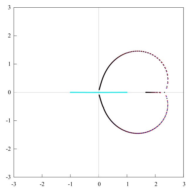
Example 1.

In this example, $p=3$, $A_{1}\in\mathbb{R}$, $A_{2}=\overline{A}_{3}\notin\mathbb{R}$, $\alpha_{1}=-2/3$, $\alpha_{2}=\alpha_{3}=1/3$ in representation (3.2). In Fig. 1, the dark (blue, red, and black) points are the zeros of the Hermite–Padé polynomial of type I $Q_{n,0}$, $Q_{n,1}$ and $Q_{n,2}$, which simulate the $S$-compact set $\mathbf{F}$ (or, more precisely, its projection $\pi(\mathbf{F})$). The arrangement of these points resembles the Chebotarev compact set of minimal capacity for three points (which is depicted after the change $z\mapsto 1/z$). The extremal property of our compact set $\mathbf{F}$ is related to the point $\mathbf{z}=\infty^{(0)}$, which lies on the zero sheet of the Riemann surface $\mathfrak{R}(f)$. The zeros of the Hermite–Padé polynomial of type II $q_{2n}$ (light blue points) simulate the second $S$-compact set $\mathbf{E}$. Since the initial data are symmetric about the real line, we have here $\pi(\mathbf{E})=[-1,1]$. However, this is not so in the general case, as we shall see from Examples 2 and 3.

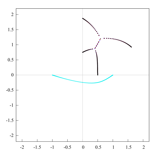
Example 2.

In this example, $f\in\mathscr{Z}(\Delta)$ is such that $p=4$ in representation (3.2), and besides, all the pairwise distinct points $a_{1},a_{2},a_{3},a_{4}$ lie in the upper half-plane. The parameters $\alpha_{1},\alpha_{2},\alpha_{3},\alpha_{4}$ are chosen so that the $S$-compact set $\mathbf{F}$ is a continuum (connecting these four points). In Fig. 2, the dark (blue, red, and black) points are the zeros of the Hermite–Padé polynomials of type I $Q_{n,0}$, $Q_{n,1}$ and $Q_{n,2}$, which simulate the compact set $\mathbf{F}$ (or, more precisely, its projection $\pi(\mathbf{F})$). As in the first example, the complement of $\mathbf{F}$ (which contains the point $\mathbf{z}=\infty^{(0)}$) is the Stahl domain $\mathfrak{D}_{1}$ on the Riemann surface $\mathfrak{R}(f)$. The compact set $\pi(\mathbf{F})$ is an analogue of the classical Chebotarev continuum for 4 points. In addition to four branch points, it also contains two Chebotarev points at which the equilibrium measure $\lambda_{F}$ has zero density. The light blue points are the zeros of the Hermite–Padé polynomials of type II $q_{2n}$, which simulate the second $S$-compact set $\mathbf{E}$. In our case, $\pi(\mathbf{E})\neq\Delta$. More precisely, $\pi(\mathbf{E})\cap\Delta=\{-1,1\}$. The complement of $\mathbf{E}$ on the Riemann surface $\mathfrak{R}(f)$ (which contains the point $\mathbf{z}=\infty^{(0)}$) is the Stahl domain $\mathfrak{D}_{0}$ (the zero sheet). The open set $\mathfrak{D}_{1}\setminus\overline{\mathfrak{D}}_{0}$ is the first sheet (in our setting, this set is connected, and hence, is a domain). But this is not always the case — corresponding examples can be constructed for a slightly more general class of functions than the class $\mathscr{Z}(\Delta)$ (see Example 4 below).

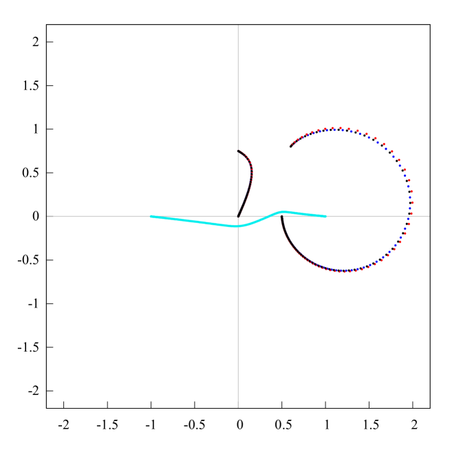
Example 3.

In this example, $f\in\mathscr{Z}(\Delta)$ is such that we again have $p=4$ in representation (3.2), the four points $a_{1},a_{2},a_{3},a_{4}$ are such that there is again no symmetry about the real line. Besides, $\alpha_{j}\in\{-1/2,1/2\}$ (the condition $\sum_{j=1}^{4}\alpha_{j}=0$ is retained). So, $f$ has branch points of order 2 only. Geometrically, the four points $a_{j}$ were chosen so that the projection $\pi(\mathbf{F})$ of the $S$-compact set $\mathbf{F}$ consists of two disjoint arcs. In Fig. 3, the dark (blue, red, and black) points are the zeros of the Hermite–Padé polynomials of type I $Q_{n,0}$, $Q_{n,1}$ and $Q_{n,2}$, which simulate the projection $\pi(\mathbf{F})$ of the compact set $\mathbf{F}$. The complement of $\mathbf{F}$ (which contains the point $\mathbf{z}=\infty^{(0)}$) is the Stahl domain $\mathfrak{D}_{1}$ on the Riemann surface $\mathfrak{R}(f)$. The light blue points represent the zeros of the Hermite–Padé polynomials of type I, which simulate the second $S$-compact set $\mathbf{E}$. In the case under consideration, $\pi(\mathbf{E})\neq\Delta$. More precisely, $\pi(\mathbf{E})\cap\Delta=\{-1,1\}$. The complement of $\mathbf{E}$ on the Riemann surface $\mathfrak{R}(f)$ (which contains the point $\mathbf{z}=\infty^{(0)}$) is the Stahl domain $\mathfrak{D}_{0}$ (the zero sheet). The open set $\mathfrak{D}_{1}\setminus\overline{\mathfrak{D}}_{0}$ is the first sheet (in our case, this set is connected, and hence, a domain).

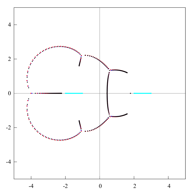
Example 4.

In this example, a more general class of multivalued analytic functions than the class $\mathscr{Z}(\Delta)$ is considered. Namely, instead of one closed interval $\Delta=[-1,1]$, we consider two disjoint real closed intervals $\Delta_{1}$ and $\Delta_{2}$ and the corresponding two inverses of the Joukowsky function $\varphi_{\Delta_{1}}(z)$ and $\varphi_{\Delta_{2}}(z)$. In this case, the multivalued function $f$ has the form

$$f(z):=\prod_{j=1}^{p}\left(A_{j}-\frac{1}{\varphi_{\Delta_{1}}(z)}\right)^{\alpha_{j}}\prod_{k=1}^{q}\left(B_{k}-\frac{1}{\varphi_{\Delta_{2}}(z)}\right)^{\beta_{k}},$$ (3.16)

where, as before, it is assumed that the quantities $A_{j}$ are pairwise disjoint, $|A_{j}|>1$, and the corresponding quantities $a_{j}$, $\varphi_{\Delta_{1}}(a_{j})=A_{j}$, are such that $a_{j}\notin(\Delta_{1}\cup\Delta_{2})$. Similar assumptions are made about the quantities $B_{k}$. Moreover, it is assumed that $a_{j}\neq b_{k}$ for all $j$ and that the points $a_{j}$, $b_{k}$ and the exponents $\alpha_{j}$, $\beta_{k}$ are such that geometrically the problem is symmetric about the real line. In this case, the results of [24] can be applied (the results of [32] are inapplicable, because this paper deals only with the class $\mathscr{Z}(\Delta)$. Under these conditions, the $S$-compact set $\mathbf{F}$ should be such that the compact set $\pi(\mathbf{F})$ is symmetric about the real line, while the second $S$-compact set $\mathbf{E}$ should be such that $\pi(\mathbf{E})=\Delta_{1}\cup\Delta_{2}$. This is fully confirmed by numerical results. In Fig. 4, the dark (blue, red, and black) points are the zeros of the Hermite–Padé polynomials of type I $Q_{n,0}$, $Q_{n,1}$ and $Q_{n,2}$, which simulate the compact set $\pi(\mathbf{F})$. The complement of $\mathbf{F}$ (which contains the point $\mathbf{z}=\infty^{(0)}$) is the Stahl domain $\mathfrak{D}_{1}$ on the Riemann surface $\mathfrak{R}(f)$. The light blue points are the zeros of the Hermite–Padé polynomials of type II $q_{2n}$, which simulate the compact set $\pi(\mathbf{E})$. In this case, $\pi(\mathbf{E})=\Delta_{1}\cup\Delta_{2}$. The complement of $\mathbf{E}$ on the Riemann surface $\mathfrak{R}(f)$ (which contains the point $\mathbf{z}=\infty^{(0)}$) is the Stahl domain $\mathfrak{D}_{0}$ (the zero sheet). The open set $\mathfrak{D}_{1}\setminus\overline{\mathfrak{D}}_{0}$ is the first sheet (in this case, this set is disconnected, and hence is not a domain). The open set $\overline{\mathbb{C}}\setminus\pi(\mathbf{F})$ consists of two domains, and hence, is not a domain. Numerical calculations have been performed with $p=2$, $A_{1}=\overline{A_{2}}\notin\mathbb{R}$ and $q=3$, $B_{1}=\overline{B}_{2}\notin\mathbb{R}$, $B_{3}\in\mathbb{R}$ in (3.16). The number of Chebotarev points of zero density is five.

It should be noted that in all above Examples 1–4 the compact set $\pi(\mathbf{F})$ is disjoint from the compact set $\pi(\mathbf{E})$ and from the closed interval $\Delta$. This is a certain heuristic principle, which always holds in the function class $\mathscr{Z}(\Delta)$ (and even in the more general function class of the form (3.16)).

4. Appendix

Lemma 2.

Let $\mu\in M_{1}(F)$ and let

$$v(z)=v(z;\mu):=\int\log\bigl{|}1-\varphi(z)\varphi(t)\bigr{|}\,d\mu(t).$$

Then

$$v(z;\mu)=-\frac{1}{2}U^{\beta_{E}(\mu)+\tau_{E}}(z)+\operatorname{const},$$ (4.1)

where $\beta_{E}(\mu)$ is the balayage of the measure $\mu$ from the domain $D$ to $E$ and $\tau_{E}$ is the Chebyshev measure of the interval $E$.

Proof.

Indeed, since the compact sets $E$ and $F$ lie on the real line $\mathbb{R}$ and since the function $\varphi(z)$ assumes real values for $z\in\mathbb{R}\setminus E$, we have, for the Green function $g_{E}(z,t)$ of the domain $D$,

$$g_{E}(z,t)=\log\frac{|1-\varphi(z)\overline{\varphi(t)}|}{|\varphi(z)-\varphi(t)|}=\log\frac{|1-\varphi(z)\varphi(t)|}{|\varphi(z)-\varphi(t)|}$$ (4.2)

for $z,t\in\mathbb{R}\setminus E$. Let us now employ the identity

$$z-a\equiv-\frac{\bigl{(}\Phi(\mathbf{z})-\Phi(\mathbf{a})\bigr{)}\bigl{(}1-\Phi(\mathbf{z})\Phi(\mathbf{a})\bigr{)}}{2\Phi(\mathbf{z})\Phi(\mathbf{a})},\quad z,a\in D,$$

which can be easily verified (see [11], [28]). Using this relation, representation (4.2), and the relation between the functions $\Phi(\mathbf{z})$ and $\varphi(z)$, we finally get

$$g_{E}(z,t)=\log\frac{|1-\varphi(z)\varphi(t)|^{2}}{2|z-t|\cdot|\varphi(z)\varphi(t)|}.$$ (4.3)

By identity (4.3), for the Green potential $G^{\mu}_{E}(z)$ of the measure $\mu\in M_{1}(F)$ we get

$$G^{\mu}_{E}(z): =\int g_{E}(z,t)\,d\mu(t)=$$

$$=2\int\log|1-\varphi(z)\varphi(t)|\,d\mu(t)+U^{\mu}(z)-\log|\varphi(z)|+\operatorname{const}$$

$$=2v(z;\mu)+U^{\mu}(z)-\gamma_{E}+U^{\tau_{E}}(z)+\operatorname{const}.$$ (4.4)

Let us apply the operator $\mathrm{dd}^{c}$ to the function $v(z;\mu)$. We have (see [5])

$$\frac{1}{2\pi}\mathrm{dd}^{c}G^{\mu}_{E}(z)=\beta_{E}(\mu)-\mu,$$

and hence, using (4.4), this establishes

$$2\pi(\beta_{E}(\mu)-\mu)=2\mathrm{dd}^{c}v(z;\mu)+2\pi(\delta_{\infty}-\mu)+2\pi(\delta_{\infty}-\tau_{E}).$$

It follows that

$$2\mathrm{dd}^{c}v(z;\mu)=2\pi(\beta_{E}(\mu)+\tau_{E}-2\delta_{\infty}).$$

Therefore,

$$v(z;\mu)=-\frac{1}{2}U^{\beta_{E}(\mu)+\tau_{E}}(z)+\operatorname{const}.$$

Lemma 2 is proved. ∎

Figure 1. Here $p=3$, $A_{1}\in\mathbb{R}$, $A_{2}=\overline{A}_{3}\notin\mathbb{R}$, $\alpha_{1}=-2/3$, $\alpha_{2}=\alpha_{3}=1/3$ in representation (3.2). The dark (blue, red, and black) points are the zeros of the Hermite–Padé polynomials of type I $Q_{350,0}$, $Q_{350,1}$ and $Q_{350,2}$, which simulate the compact set $\pi(\mathbf{F})$. The arrangement of these points resembles the Chebotarev compact set of minimal capacity for three points (which is depicted after the change $z\mapsto 1/z$). The extremal property of our compact set $\mathbf{F}$ is related to the point $\mathbf{z}=\infty^{(0)}$, which lies on the zero sheet of the Riemann surface $\mathfrak{R}(f)$. The zeros of the Hermite–Padé polynomial of type II $q_{100}$ (light blue points) simulate the second compact set $\pi(\mathbf{E})$. Since the initial data are symmetric about the real line, we have here $\pi(\mathbf{E})=[-1,1]$. However, this is not so in the general case, as we shall see from Figs. 2 and 3.

Figure 2. Here in (3.2) we take $p=4$. All the four points $a_{1},a_{2},a_{3},a_{4}$ lie in the upper half-plane, $\alpha_{1}=\alpha_{2}=1/5$, $\alpha_{3}=\alpha_{4}=-1/5$. The corresponding compact set $\mathbf{F}$ is a continuum. The dark (blue, red, and black) points are the zeros of the Hermite–Padé polynomials of type I $Q_{200,0}$, $Q_{200,1}$ and $Q_{200,2}$. These points simulate the compact set $\pi(\mathbf{F})$. The compact set $\pi(\mathbf{F})$ is an analogue of the classical Chebotarev continuum for 4 points. In addition to four branch points, it also contains two Chebotarev points of zero density. The light blue points are the zeros of the Hermite–Padé polynomials of type II $q_{100}$, which simulate the second compact set $\pi(\mathbf{E})$. In this case, $\pi(\mathbf{E})\cap\Delta=\{-1,1\}$.

Figure 3. Here in (3.2) we take $p=4$. The four points $a_{1},a_{2},a_{3},a_{4}$ are such that there is again no symmetry about the real line. Besides, $\alpha_{j}\in\{-1/2,1/2\}$ (the condition $\sum_{j=1}^{4}\alpha_{j}=0$ is retained). So, $f$ has branch points of order 2 only. Geometrically, the four points $a_{j}$ were chosen so that the compact set $\pi(\mathbf{F})$ consists of two disjoint arcs. The dark (blue, red, and black) points are the zeros of the Hermite–Padé polynomials of type I $Q_{150,0}$, $Q_{150,1}$ and $Q_{150,2}$; these points simulate the compact set $\pi(\mathbf{F})$. The light blue points represent the zeros of the Hermite–Padé polynomial of type II $q_{200}$, which simulate the compact set $\pi(\mathbf{E})$. In this case, $\pi(\mathbf{E})\cap\Delta=\{-1,1\}$.

Figure 4. In this numerical example, the class of multivalued analytic functions defined by representation (3.16) is considered. We consider two disjoint real closed intervals $\Delta_{1}$ and $\Delta_{2}$ and the corresponding two inverses of the Joukowsky function $\varphi_{\Delta_{1}}(z)$ and $\varphi_{\Delta_{2}}(z)$. It is assumed that the points $a_{j}$, $b_{k}$ and the exponents $\alpha_{j}$, $\beta_{k}$ are such that geometrically the problem is symmetric about the real line. In this case, the compact set $\pi(\mathbf{F})$ should be symmetric about the real line, and the second compact set is $\pi(\mathbf{E})=\Delta_{1}\cup\Delta_{2}$. This is fully confirmed by numerical results. The dark (blue, red, and black) points are the zeros of the Hermite–Padé polynomials of type I  $Q_{350,0}$, $Q_{350,1}$ and $Q_{350,2}$, which simulate the compact set $\pi(\mathbf{F})$. The light blue points are the zeros of the Hermite–Padé polynomial of type II $q_{100}$, which simulate the compact set $\pi(\mathbf{E})$. Numerical calculations have been performed with $p=2$, $A_{1}=\overline{A_{2}}\notin\mathbb{R}$ and $q=3$, $B_{1}=\overline{B}_{2}\notin\mathbb{R}$, $B_{3}\in\mathbb{R}$ in (3.16). The number of Chebotarev points of zero density is five; this number agrees with that of the branch points that differ from the points $z=\pm 1$.

References

- [1] A. I. Aptekarev, V. G. Lysov, “Systems of Markov functions generated by graphs and the asymptotics of their Hermite-Padé approximants”, Sb. Math., 201:2 (2010), 183–234.
- [2] A. I. Aptekarev, A. I. Bogolyubskii, M. Yattselev, “Convergence of ray sequences of Frobenius-Padé approximants”, Sb. Math., 208:3 (2017), 313–334
- [3] Baker, George A., Jr.; Graves-Morris, Peter, Padé approximants, Second edition, Encyclopedia of Mathematics and its Applications, 59, Cambridge University Press, Cambridge, 1996, xiv+746 pp. ISBN: 0-521-45007-1.
- [4] D. Barrios Rolanía, J. S. Geronimo, G. López Lagomasino, “High-order recurrence relations, Hermite-Padé approximation and Nikishin systems”, Sb. Math., 209:3 (2018), 385–420.
- [5] E. M. Chirka, “Potentials on a compact Riemann surface”, Proc. Steklov Inst. Math., 301 (2018), 272–303.
- [6] E. M. Chirka, “Equilibrium measures on a compact Riemann surface”, Proc. Steklov Inst. Math., 306 (2019), in print.
- [7] A. A. Gonchar, E. A. Rakhmanov, “On the convergence of simultaneous Padé approximants for systems of functions of Markov type”, Proc. Steklov Inst. Math., 157 (1983), 31–50.
- [8] A. A. Gonchar, E. A. Rakhmanov, “Equilibrium distributions and degree of rational approximation of analytic functions”, Math. USSR-Sb., 62:2 (1989), 305–348.
- [9] A. A. Gonchar, E. A. Rakhmanov, V. N. Sorokin, “Hermite–Padé approximants for systems of Markov-type functions”, Sb. Math., 188:5 (1997), 671–696.
- [10] A. A. Gonchar, “Rational Approximations of Analytic Functions”, Proc. Steklov Inst. Math., 272, suppl. 2 (2011), S44–S57.
- [11] A. A. Gonchar, S. P. Suetin, “On Padé approximants of Markov-type meromorphic functions”, Proc. Steklov Inst. Math., 272, suppl. 2 (2011), S58–S95.
- [12] A. A. Gonchar, E. A. Rakhmanov, S. P. Suetin, “Padeé-Chebyshev approximants of multivalued analytic functions, variation of equilibrium energy, and the S-property of stationary compact sets”, Russian Math. Surveys, 66:6 (2011), 1015–1048.
- [13] A. V. Komlov, R. V. Palvelev, S. P. Suetin, E. M. Chirka, “Hermite-Padé approximants for meromorphic functions on a compact Riemann surface”, Russian Math. Surveys, 72:4 (2017), 671–706.
- [14] A. López-Garcia and G. López Lagomasino, “Nikishin systems on star-like sets: Ratio asymptotics of the associated multiple orthogonal polynomials”, J. Approx. Theory, 225 (2018), 1–40.
- [15] A. López-Garcia and G. López Lagomasino, Nikishin systems on star-like sets: Ratio asymptotic formulae for the associated multiple orthogonal polynomials, 2019, 27 pp., arxiv:1907.03002.
- [16] G. López Lagomasino, S. Medina Peralta, J. Szmigielski, “Mixed type Hermite-Padé approximation inspired by the Degasperis-Procesi equation”, 20 June 2019, Advances in Mathematics, 349, 813–838.
- [17] A. López-Garcia, E. Mina-Diaz, “Nikishin systems on star-like sets: algebraic properties and weak asymptotics of the associated multiple orthogonal polynomials”, Sb. Math., 209:7 (2018), 1051–1088.
- [18] Guillermo López Lagomasino, Walter Van Assche, “Riemann-Hilbert analysis for a Nikishin system”, Sb. Math., 209:7 (2018), 1019–1050.
- [19] Toshiyuki Mano, Teruhisa Tsuda, “Hermite-Padé approximation, isomonodromic deformation and hypergeometric integral”, Mathematische Zeitschrift, 285:1–2 (2017), 397–431.
- [20] Andrei Martínez-Finkelshtein, Evguenii A. Rakhmanov, Sergey P. Suetin, “Asymptotics of type I Hermite-Padé polynomials for semiclassical functions”, Modern trends in constructive function theory, Contemp. Math., 661, 2016, 199–228.
- [21] E. M. Nikishin, “Asymptotic behavior of linear forms for simultaneous Padé approximants”, Soviet Math. (Iz. VUZ), 30:2 (1986), 43–52.
- [22] Nikishin, E. M., Sorokin, V. N. Rational approximations and orthogonality, Nauka, Moscow, 1988, 256 pp.
- [23] J. Nuttall, “Asymptotics of diagonal Hermite–Padé polynomials”, J. Approx.Theory, 42 (1984), 299–386.
- [24] E. A. Rakhmanov, S. P. Suetin, “The distribution of the zeros of the Hermite-Padé polynomials for a pair of functions forming a Nikishin system”, Sb. Math., 204:9 (2013), 1347–1390.
- [25] E. A. Rakhmanov, “Zero distribution for Angelesco Hermite-Padé polynomials”, Russian Math. Surveys, 73:3 (2018), 457–518.
- [26] H. Stahl, “Three different approaches to a proof of convergence for Padé approximants”, Rational approximation and applications in mathematics and physics, Łańcut, 1985, Lecture Notes in Math., 1237, Springer, Berlin, 1987, 79–124.
- [27] H. Stahl, “Asymptotics of Hermite–Padé polynomials and related convergence results. A summary of results”, Nonlinear numerical methods and rational approximation (Wilrijk, 1987), Math. Appl., 43, Reidel, Dordrecht, 1988, 23–53; also the fulltext preprint version is avaible, 79 pp.
- [28] S. P. Suetin, “On a new approach to the problem of distribution of zeros of Hermite-Padé polynomials for a Nikishin system”, Proc. Steklov Inst. Math., 301 (2018), 245–261.
- [29] S. P. Suetin, “Distribution of the zeros of Hermite-Padé polynomials for a complex Nikishin system”, Russian Mathematical Surveys, 73:2 (2018), 363–365.
- [30] Sergey P. Suetin, Hermite-Padé polynomials and analytic continuation: new approach and some results, 2018, 45 pp., arxiv:1806.08735.
- [31] S. P. Suetin, “On an Example of the Nikishin System”, Math. Notes, 104:6 (2018), 905–914.
- [32] S. P. Suetin, “Existence of a three-sheeted Nutall surface for a certain class of infinite-valued analytic functions”, Russian Math. Surveys, 74:2 (2019), 363–365.
- [33] S. P. Suetin, “On the equivalence of scalar and vector equilibrium problems for a pair of functions forming the Nikishin system”, Math. Notes, 106:6 (2019), 904–916.
- [34] Antonio Trias, “HELM: The Holomorphic Embedding Load-Flow Method: Foundations and Implementations”, Foundations and Trends in Electric Energy Systems, 3:3-4, 140–370.
- [35] Van Assche, Walter, “Pade and Hermite-Padé approximation and orthogonality”, Surv. Approx. Theory, 2 (2006), 61–91.