DQ Robotics: a Library for Robot Modeling and Control

Abstract

Dual quaternion algebra and its application to robotics have gained considerable interest in the last two decades. Dual quaternions have great geometric appeal and easily capture physical phenomena inside an algebraic framework that is useful for both robot modeling and control. Mathematical objects, such as points, lines, planes, infinite cylinders, spheres, coordinate systems, twists, and wrenches are all well defined as dual quaternions. Therefore, simple operators are used to represent those objects in different frames and operations such as inner products and cross products are used to extract useful geometric relationships between them. Nonetheless, the dual quaternion algebra is not widespread as it could be, mostly because efficient and easy-to-use computational tools are not abundant and usually are restricted to the particular algebra of quaternions. To bridge this gap between theory and implementation, this paper introduces DQ Robotics, a library for robot modeling and control using dual quaternion algebra that is easy to use and intuitive enough to be used for self-study and education while being computationally efficient for deployment on real applications.

I Introduction

Dual quaternion algebra and its application to robotics have gained considerable interest in the last two decades. Far from being an abstract mathematical tool, dual quaternions have great geometric appeal and easily capture physical phenomena inside an algebraic framework that is useful for both robot modeling and control. Mathematical objects, such as points, lines, planes, infinite cylinders, spheres, coordinate systems, twists, and wrenches are all well defined as dual quaternions. Therefore, simple operators are used to represent those objects in different coordinate systems and operations such as inner products and cross products are used to extract useful geometric relationship between them. Some authors consider the particular set of dual quaternions with unit norm, known as unit dual quaternions, as the most efficient and compact tool to describe rigid transformations [1, 2]. For instance, homogeneous transformation matrices (HTM) have sixteen elements, whereas dual quaternions have eight elements and dual quaternion multiplications are less expensive than HTM multiplications [3, p. 42]. Moreover, it is easy to extract geometric parameters from a given unit dual quaternion (translation, axis of rotation, angle of rotation). Nonetheless, they are easily mapped into a vector structure, which can be particularly convenient to perform tasks such as pose control as there is no need to extract parameters from the dual quaternion.

Nonetheless, the dual quaternion algebra is not widespread as it could be, not only because classic matrix algebra on real numbers is very mature and it is the backbone of most robotics textbooks [4, 5, 6], but also because efficient and easy-to-use computational tools are not abundant and usually are restricted to the particular algebra of quaternions. Indeed, the Boost Math library implements quaternions and even octonions, but not dual quaternions, whereas the Eigen library implements only quaternions, both in C++ language. Some libraries also implement dual quaternions in Lua, MATLAB [7], and C++, but none of them are focused on robotics.

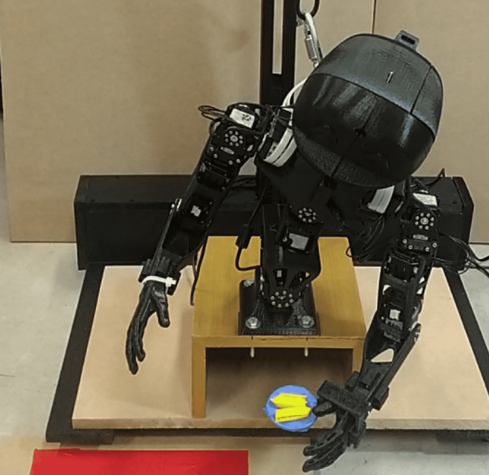
This paper introduces DQ Robotics, a library for robot modeling and control using dual quaternion algebra that is computationally efficient, easy to use, and is intuitive enough to be used for self-study and education and sufficiently efficient for deployment on real applications. For instance, DQ Robotics has already been used in real platforms such as cooperative manipulators for surgical applications, mobile manipulators, and humanoids, among several other robotic systems, some of which are shown in Fig. 10. It is written in three languages, namely Python, MATLAB, and C++, all of them sharing a unified programming style to make the transition from one language to another as smooth as possible, enabling fast prototype-to-release cycles. Furthermore, a great effort has been made to make coding as close as possible to the mathematical notation used on paper, making it easy to implement code as soon as one has grasped the mathematical concepts.

DQ Robotics uses the expressiveness of dual quaternion algebra for both robot modeling and control. This paper introduces the main features of the library as well as its basic usage in a tutorial-like style. The tutorial begins with the presentation of dual quaternion notation and basic operations, goes through robot modeling and control, and ends with a complete robot control example of two robots cooperating in a task where one manipulator robot and a mobile manipulator interact while deviating from obstacles in the workspace.

I-A How to follow the tutorial

In this paper, for brevity, we present several code snippets in MATLAB language that should be familiar to most roboticists. Suitable commands are also available in Python and C++. The readers might be interested in downloading and installing the DQ Robotics toolbox for MATLAB and trying out the code snippets in their own machine. More details are given in Section VIII and in the DQ Robotics documentation.

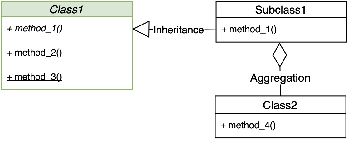
The tutorial also has a few diagrams using the Unified Modeling Language (UML), which we use to explain the object-oriented modeling of the library in a way that is agnostic to the programming language. A simplified UML diagram that shows the relevant object-oriented concepts used in this paper is briefly explained in Fig. 1.

Figure 1: A simplified class diagram in the Unified Modeling Language (UML). Abstract methods and classes are italicized. Concrete methods and classes are in upright text. Static method are underlined. Specific arrowheads indicate inheritance and aggregation.

I-B Notation choice and common operations

Given the imaginary units $\hat{\imath}$,$\hat{\jmath}$,$\hat{k}$ that satisfy $\hat{\imath}^{2}=\hat{\jmath}^{2}=\hat{k}^{2}=\hat{\imath}\hat{\jmath}\hat{k}=-1$ and the dual unit $\varepsilon$, which satisfies $\varepsilon\neq 0$ and $\varepsilon^{2}=0$, the quaternion set is defined as

$$\mathbb{H}\triangleq\left\{h_{1}+\hat{\imath}h_{2}+\hat{\jmath}h_{3}+\hat{k}h_{4}\,:\,h_{1},h_{2},h_{3},h_{4}\in\mathbb{R}\right\}$$

and the dual quaternion set is defined as

$$\mathcal{H}\triangleq\left\{\boldsymbol{h}_{1}+\varepsilon\boldsymbol{h}_{2}\,:\,\boldsymbol{h}_{1},\boldsymbol{h}_{2}\in\mathbb{H}\right\}.$$

There are several equivalent notations for representing dual quaternions, but we adopt the hypercomplex one, which regards them as an extension of complex numbers. This way, sums, multiplications and subtractions are exactly the same used in complex numbers (and also in real numbers!), differently from the scalar-plus-vector notation, which requires the redefinition of the multiplication operation. When designing DQ Robotics, one important guiding principle was to be able to use dual quaternion operations as close as possible to the way that we do it on paper, closing the gap between theory and implementation.

For instance, the dual quaternions $\underline{\boldsymbol{a}}=\hat{\imath}+\varepsilon\left(1+\hat{k}\right)$ and $\underline{\boldsymbol{b}}=-2+\hat{\jmath}+\varepsilon\left(\hat{\imath}+\hat{k}\right)$ are declared in MATLAB as

⬇

a = DQ.i + DQ.E*(1 + DQ.k);

b = -2 + DQ.j + DQ.E*(DQ.i + DQ.k);

and

⬇

>> a + b

ans = ( - 2 + 1i + 1j) + E*(1 + 1i + 2k)

>> a * b

ans = ( - 2i + 1k) + E*( - 3 - 1i - 2k)

Alternatively, one can use include_namespace_dq to enable the aliases i_, j_, k_, and E_. Therefore,

⬇

>> E_*a

ans = E*(1i)

The list of the main DQ class operations is shown in Table I.

TABLE I: Main methods of class DQ.

Binary operations between two dual quaternions (e.g., a + b)
+, -,*	Sum, subtraction, and multiplication.
/, \	Right division and left division.
Unary operations (e.g., -a and a’)
-	Minus.
[’], [.’]	Conjugate and sharp conjugate.
Unary operators (e.g., P(a))
conj, sharp	Conjugate and sharp conjugate.
exp, log	Exponential of pure dual quaternions and logarithm of unit dual quaternions.
inv	Inverse under multiplication.
hamiplus4, haminus4	Hamilton operators of a quaternion.
hamiplus8, haminus8	Hamilton operators of a dual quaternion.
norm	Norm of dual quaternions.
P, D	Primary part and dual part.
Re, Im	Real component and imaginary components.
rotation	Rotation component of a unit dual quaternion.
rotation_axis, rotation_angle	Rotation axis and rotation angle of a unit dual quaternion.
vec3, vec6	Three-dimensional and six-dimensional vectors composed of the coefficients of the imaginary part of a quaternion and a dual quaternion, respectively.
vec4, vec8	Four-dimensional and eight-dimensional vectors composed of the coefficients of a quaternion and a dual quaternion, respectively.
Binary operators (e.g., Ad(a,b))
Ad, Adsharp	Adjoint operation and sharp adjoint.
cross, dot	Cross product and dot product.
Binary relations (e.g. a == b)
==, ~=	Equal and not equal.
Common methods
[plot]	Plots coordinate systems, lines, and planes.

*Methods and operations enclosed by brackets (e.g., [.*]) are available only on MATLAB.

II Representing rigid motions

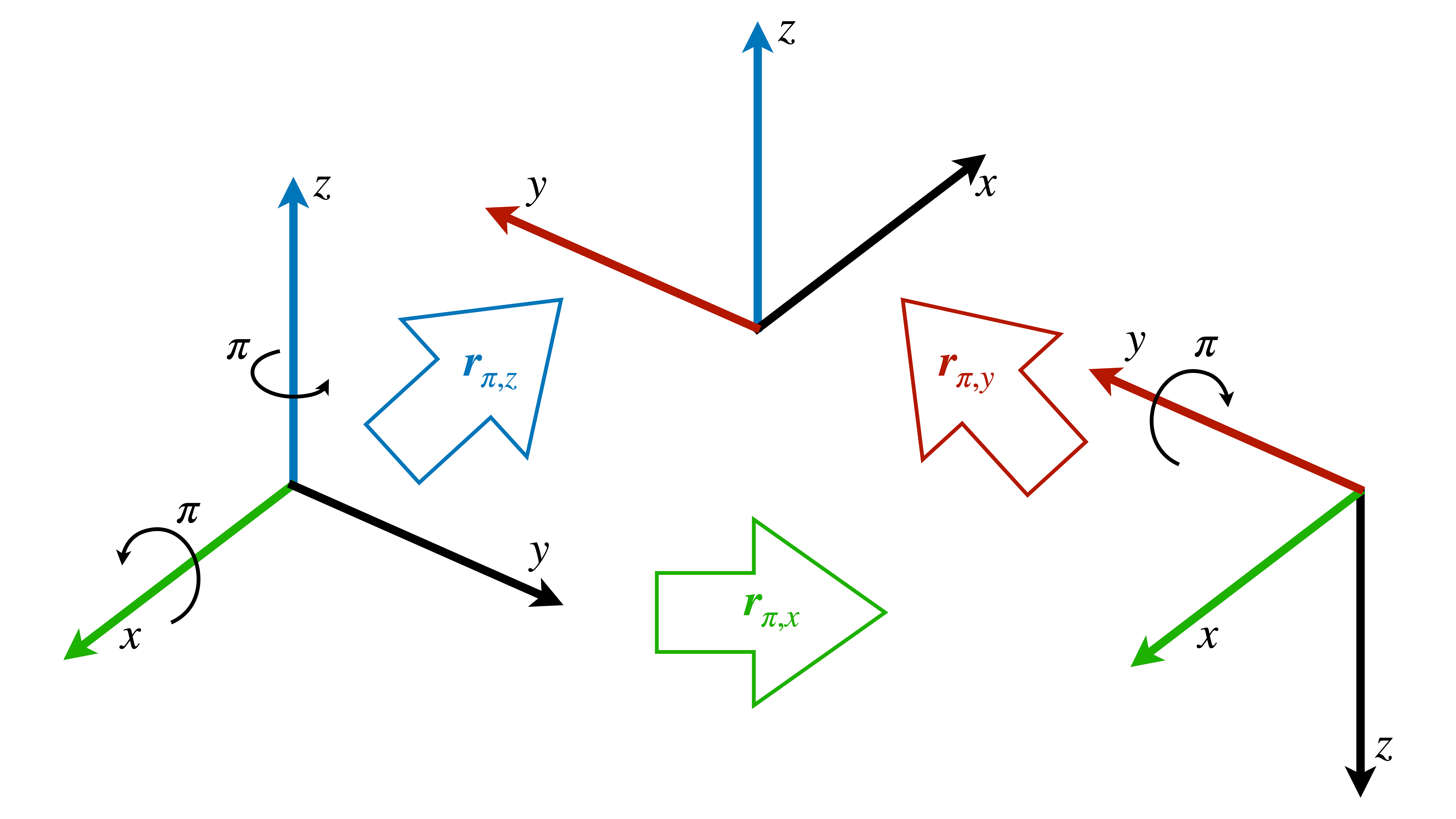
Since the set of dual quaternions represents an eight-dimensional space, it is particularly useful to represent rotations, translations, and, more generally, rigid motions. For instance, the set $\mathbb{S}^{3}\triangleq\left\{\boldsymbol{h}\in\mathbb{H}:\left\|\boldsymbol{h}\right\|=1\right\}$ is used to represent rotations, with $\left\|\boldsymbol{h}\right\|\triangleq\sqrt{\boldsymbol{h}\boldsymbol{h}^{*}}=\sqrt{h_{1}^{2}+h_{2}^{2}+h_{3}^{2}+h_{4}^{2}}$ being the quaternion norm and $\boldsymbol{h}^{*}=h_{1}-(h_{2}\hat{\imath}+h_{3}\hat{\jmath}+h_{4}\hat{k})$ being the conjugate of $\boldsymbol{h}=h_{1}+h_{2}\hat{\imath}+h_{3}\hat{\jmath}+h_{4}\hat{k}$. Any element $\boldsymbol{r}\in\mathbb{S}^{3}$ can always be written as $\boldsymbol{r}=\cos\left(\phi/2\right)+\boldsymbol{n}\sin\left(\phi/2\right)$, where $\boldsymbol{n}=n_{x}\hat{\imath}+n_{y}\hat{\jmath}+n_{z}\hat{k}\in\mathbb{S}^{3}$ is the unit-norm rotation axis and $\phi\in[0,2\pi)$ is the rotation angle. Therefore, a rotation of $\pi$ rad around the $x$-axis is given by $\boldsymbol{r}_{\pi,x}\triangleq\cos(\pi/2)+\hat{\imath}\sin(\pi/2)=\hat{\imath}.$

Since the multiplication of unit quaternions is also a unit quaternion, a sequence of rotations is given by a sequence of multiplications of unit quaternions. For instance, if first we perform the rotation $\boldsymbol{r}_{\pi,x}$ and then we use the rotated frame to do another rotation of $\pi$ rad around the $y$-axis, given by $\boldsymbol{r}_{\pi,y}\triangleq\cos(\pi/2)+\hat{\jmath}\sin(\pi/2)=\hat{\jmath}$, then the final rotation is given by $\boldsymbol{r}_{\pi,x}\boldsymbol{r}_{\pi,y}=\hat{\imath}\hat{\jmath}=\hat{k}$ because $\hat{\imath}\hat{\jmath}\hat{k}=-1$ and $\hat{k}^{2}=-1$. Besides, because $\hat{k}=\cos(\pi/2)+\hat{k}\sin(\pi/2)$, then $\boldsymbol{r}_{\pi,x}\boldsymbol{r}_{\pi,y}=\boldsymbol{r}_{\pi,z}$, which represents the rotation of $\pi$ rad around the $z$-axis. This is illustrated in Fig. 2.

Figure 2: Sequence of rotations represented by multiplication of unit quaternions. Each arrow has the same color of the rotation axis.

The set of pure quaternions is defined as $\mathbb{H}_{p}\triangleq\left\{h_{1}\hat{\imath}+h_{2}\hat{\jmath}+h_{3}\hat{k}:h_{1},h_{2},h_{3}\in\mathbb{R}\right\}\subset\mathbb{H}$ and is used to represent elements of a tridimensional space. For instance, the point $\left(x,y,z\right)$ can be directly mapped to $x\hat{\imath}+y\hat{\jmath}+z\hat{k}$, which is an element of $\mathbb{H}_{p}$. Furthermore, given a point $\boldsymbol{p}^{0}\in\mathbb{H}_{p}$ in frame $\mathcal{F}_{0}$ and the unit quaternion $\boldsymbol{r}_{1}\in\mathbb{S}^{3}$ that represents the rotation from $\mathcal{F}_{0}$ to $\mathcal{F}_{1}$, the coordinates of the point in $\mathcal{F}_{1}$ is $\boldsymbol{p}^{1}=\boldsymbol{r}_{1}^{*}\boldsymbol{p}^{0}\boldsymbol{r}_{1}$. Analogously, given $\boldsymbol{r}_{2}\in\mathbb{S}^{3}$ that represents the rotation from $\mathcal{F}_{1}$ to $\mathcal{F}_{2}$, the coordinates of the point in $\mathcal{F}_{2}$ is $\boldsymbol{p}^{2}=\boldsymbol{r}_{2}^{*}\boldsymbol{p}^{1}\boldsymbol{r}_{2}=\boldsymbol{r}_{2}^{*}\boldsymbol{r}_{1}^{*}\boldsymbol{p}^{0}\boldsymbol{r}_{1}\boldsymbol{r}_{2}$, which implies that the unit quaternion that represent the rotation from $\mathcal{F}_{0}$ to $\mathcal{F}_{2}$ is given by $\boldsymbol{r}_{1}\boldsymbol{r}_{2}$, showing again that a sequence of rotations is given by multiplication of unit quaternions.

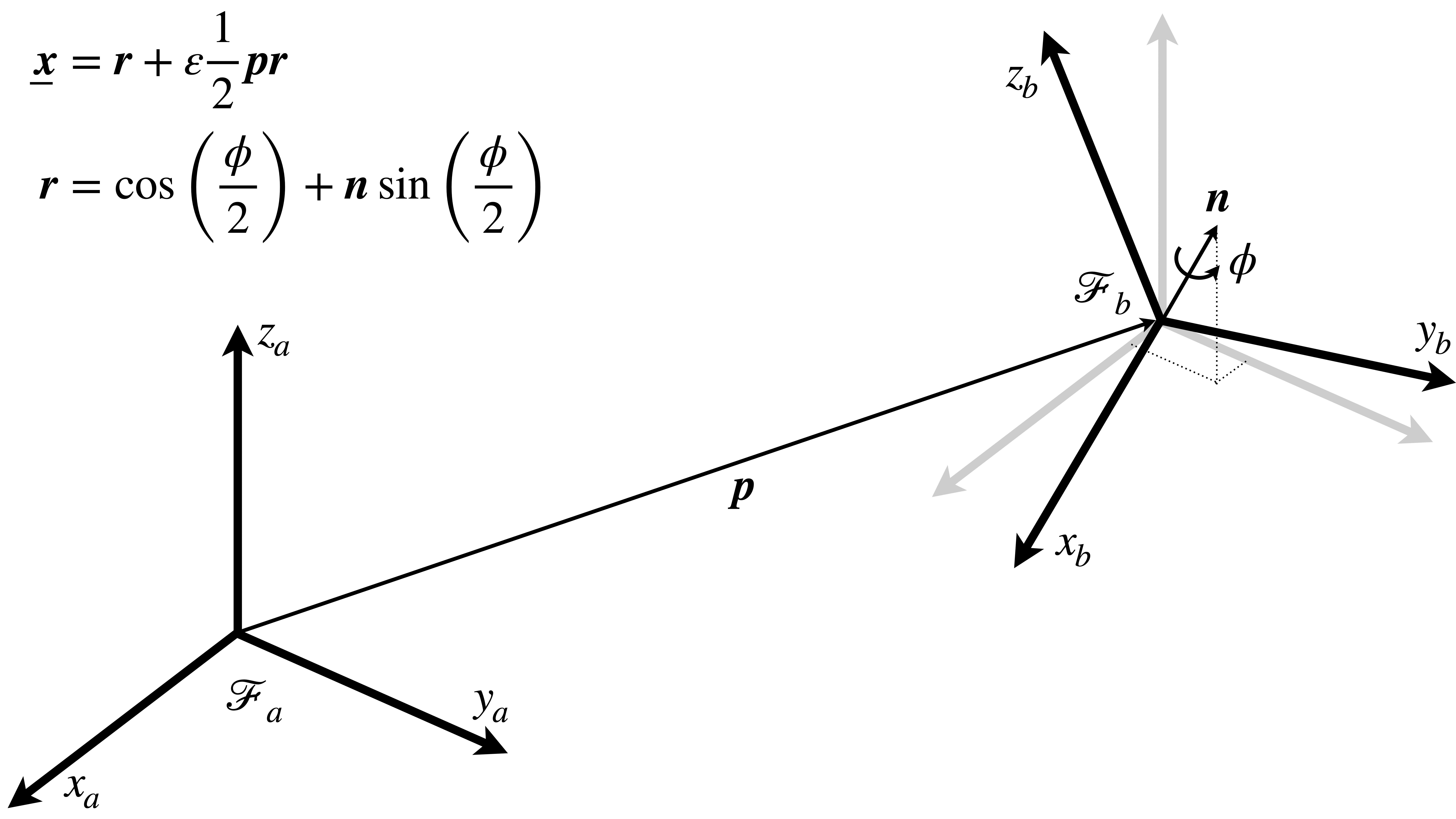
Translations and rotations can be grouped into a single unit dual quaternion. More specifically, a rigid motion is represented by

$$\underline{\boldsymbol{x}} =\boldsymbol{r}+\varepsilon\frac{1}{2}\boldsymbol{p}\boldsymbol{r},$$ (1)

as illustrated in Fig. 3, and a sequence of rigid motions is given by multiplication of unit dual quaternions. For a more detailed description of the fundamentals of dual quaternion algebra, see [8].

Figure 3: A rigid motion $\underline{\boldsymbol{x}}$ between frames $\mathcal{F}_{a}$ and $\mathcal{F}_{b}$ given by a translation $\boldsymbol{p}$ followed by a rotation $\boldsymbol{r}$.

Using DQ Robotics, a translation of $\left(0.1,0.2,0.3\right)\mathrm{m}$ followed by a rotation of $\pi$ rad around the $y$-axis, using (1), is declared in MATLAB as

Listing 1: Declaring a unit dual quaternion in MATLAB.

⬇

r = cos(pi/2) + j_*sin(pi/2);

p = 0.1*i_ + 0.2*j_ + 0.3*k_;

xd = r + E_*0.5*p*r;

Alternatively, one could declare the rotation and translation as

⬇

r = DQ([cos(pi/2), 0, sin(pi/2), 0]);

p = DQ([0, 0.1, 0.2, 0.3]);

Whereas the first way is closer to the mathematical notation, the second one can be convenient when using the matrix functions available in MATLAB, Python, and C++.

III Robot kinematics

The implementation of robot kinematic modeling is done by means of the abstract class DQ_Kinematics and all its subclasses, whose hierarchy is shown in Fig. 4. The library currently supports serial manipulators, mobile bases and their composition, which results in mobile manipulators (managed by the DQ_WholeBody class), bimanual systems (managed by the DQ_CooperativeDualTaskSpace class) and even branched mechanisms such as bimanual mobile manipulators. Common manipulator robots are available, such as the KUKA LWR4 and the Barrett WAM Arm, but custom robots can be easily created by using arbitrary Denavit-Hartenberg parameters. Some common mobile robots, such as the differential-drive iRobot Create, are also available. Creating new ones requires only the wheels radiuses and the axis length.

Let us consider the KUKA YouBot, which is a mobile manipulator composed of a 5-DOF manipulator serially coupled to a holonomic base. One easy way of defining it on DQ Robotics is to model the arm and the mobile base separately and then assemble them to form a mobile manipulator. The serial arm is defined, with the help of the Denavit-Hartenberg parameters, as follows:

⬇

arm_DH_theta = [0, pi/2, 0, pi/2, 0];

arm_DH_d = [0.147, 0, 0, 0, 0.218];

arm_DH_a = [0, 0.155, 0.135, 0, 0];

arm_DH_alpha = [pi/2, 0, 0, pi/2, 0];

arm_DH_matrix = [arm_DH_theta; arm_DH_d; arm_DH_a;

arm_DH_alpha];

arm = DQ_SerialManipulator(arm_DH_matrix,’standard’);

The holonomic base is defined as

⬇

base = DQ_HolonomicBase();

and then they are coupled together in a DQ_WholeBody object:

⬇

x_bm = 1 + E_*0.5*(0.22575*i_ + 0.1441*k_);

base.set_frame_displacement(x_bm);

robot = DQ_WholeBody(base);

robot.add(arm);

Since there is a displacement between the mobile base frame and the location where the arm is attached, we use the method set_frame_displacement(). New kinematic chains can be serially coupled to the last chain by using the method add().

Because the KUKA Youbot is already defined in DQ Robotics, it suffices to instantiate an object of the KukaYoubot class:

⬇

youbot = KukaYoubot.kinematics();

All standard robots in DQ Robotics are defined inside the folder [root_folder]/robots and have the static method kinematics() that returns a DQ_Kinematics object. Therefore, a KUKA LWR 4 robot manipulator can be defined analogously:

⬇

lwr4 = KukaLwr4Robot.kinematics();

All DQ_Kinematics subclasses have common functions for robot kinematics such as the ones used to calculate the forward kinematics, the Jacobian matrix that maps the configuration velocities to the time-derivative of the end-effector pose, as well as other Jacobian matrices that map the configuration velocities to the time derivative of other geometrical primitives attached to the end-effector, such as lines and planes. This includes DQ_WholeBody objects, therefore the corresponding Jacobians are whole-body Jacobians that take into account the complete kinematic chain. The list of the main methods is summarized in the simplified UML diagram in Fig. 4 and detailed in Table II.

Figure 4: Simplified UML class diagram of the robot modeling classes with the main methods that are available in C++, Python and MATLAB.

TABLE II: Main methods of class DQ_Kinematics and its subclasses.

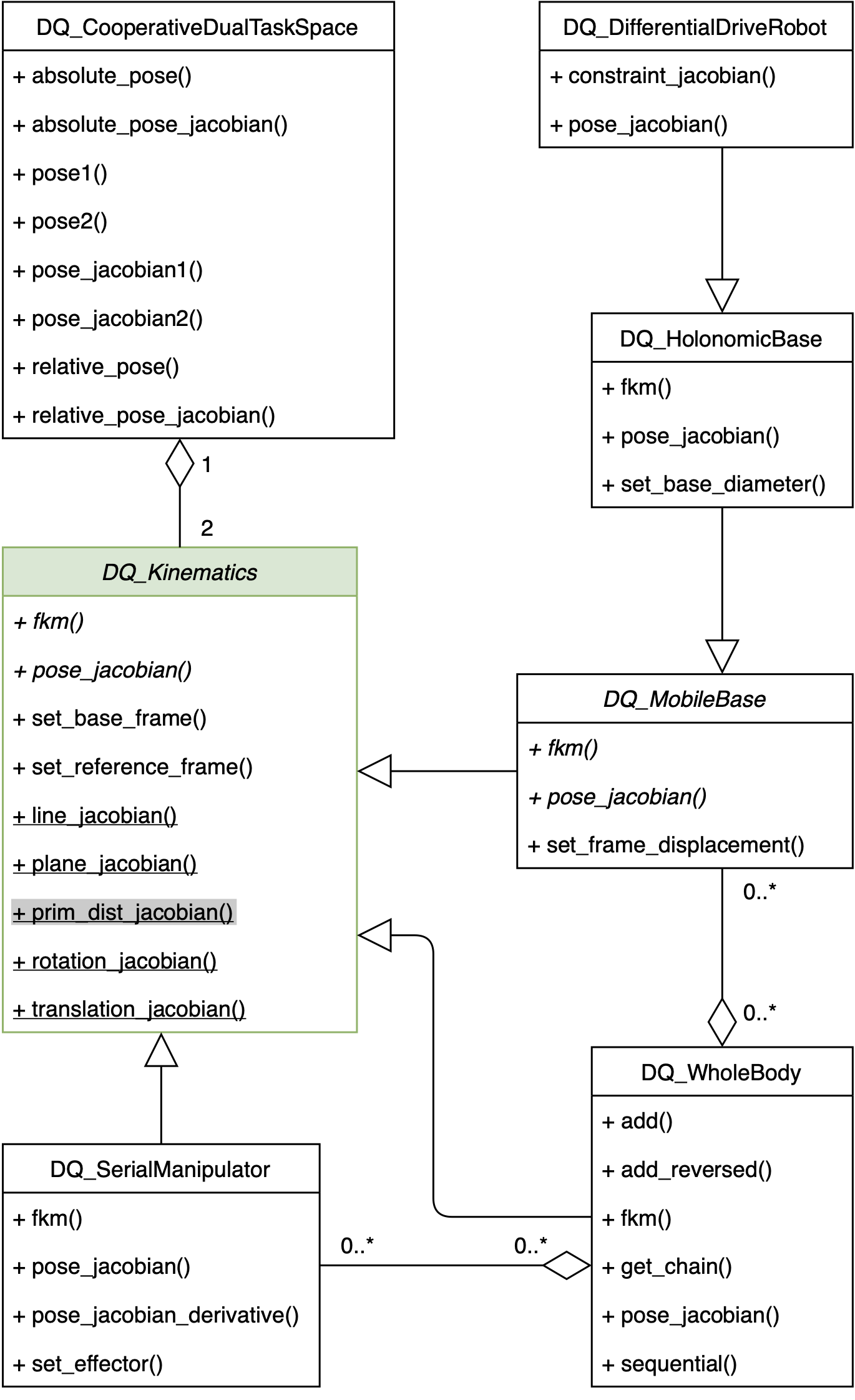
DQ_Kinematics
fkm	Compute the forward kinematics.
pose_jacobian	Compute the Jacobian that maps the configurations velocities to the time derivative of the pose of a frame attached to the robot.
set_base_frame	Set the physical location of the robot in space.
set_reference_frame	Set the reference frame for all calculations.
line_jacobian	Compute the Jacobian that maps the configurations velocities to the time derivative of a line attached to the robot.
plane_jacobian	Compute the Jacobian that maps the configurations velocities to the time derivative of a plane attached to the robot.
rotation_jacobian	Compute only the rotational part of the pose_jacobian.
translation_jacobian	Compute only the translational part of the pose_jacobian.
{prim_dist_jacobian}	Compute the Jacobian that maps the configurations velocities to the time derivative of the distance between a primitive attached to the robot and another primitive in the workspace. For instance, {prim_dist_jacobian} can be line_to_line_distance_jacobian, line_to_point_distance_jacobian, plane_to_point_distance_jacobian, point_to_line_distance_jacobian, point_to_plane_distance_jacobian, point_to_point_distance_jacobian.
DQ_SerialManipulator
pose_jacobian_derivative	Compute the analytical time derivative of the pose Jacobian matrix.
set_effector	Set a constant transformation for the end-effector pose with respect to the frame attached to the end of the last link.
DQ_MobileBase, DQ_HolonomicBase, and DQ_DifferentialDriveRobot
set_frame_displacement	Set the rigid transformation for the base frame.
set_base_diameter	Change the base diameter.
constraint_jacobian	Compute the Jacobian that relates the wheels velocities to the configuration velocities.
DQ_WholeBody
add	Add a new element to the end of the serially coupled kinematic chain.
add_reversed	Add a new element, but in reverse order, to the end of the serially coupled kinematic chain.
get_chain	Returns the complete kinematic chain.
sequential	Reorganize a sequential configuration vector in the ordering required by each kinematic chain (i.e., the vector blocks corresponding to reversed chains are reversed).
DQ_CooperativeDualTaskSpace
absolute_pose	Compute the pose of a frame between the two end-effectors, which is usually related to a grasped object.
absolute_pose_jacobian	Compute the Jacobian that maps the joint velocities of the two-arm system to the time derivative of the absolute pose.
pose1 and pose2	Compute the poses of the first and second end-effectors, respectively.
pose_jacobian1 and pose_jacobian2	Compute the Jacobians that maps the configurations velocities to the time derivative of the poses of the first and second end-effectors, respectively.
relative_pose	Compute the rigid transformation between the two end-effectors.
relative_pose_jacobian	Compute the Jacobian that maps the joint velocities of the two-arm system to the time derivative of the relative pose.

*Abstract methods are written in italics, concrete methods are written in upright, and static methods are underlined. Concrete methods that implement their abstract counterparts are omitted for the sake of conciseness.

IV Geometric Primitives

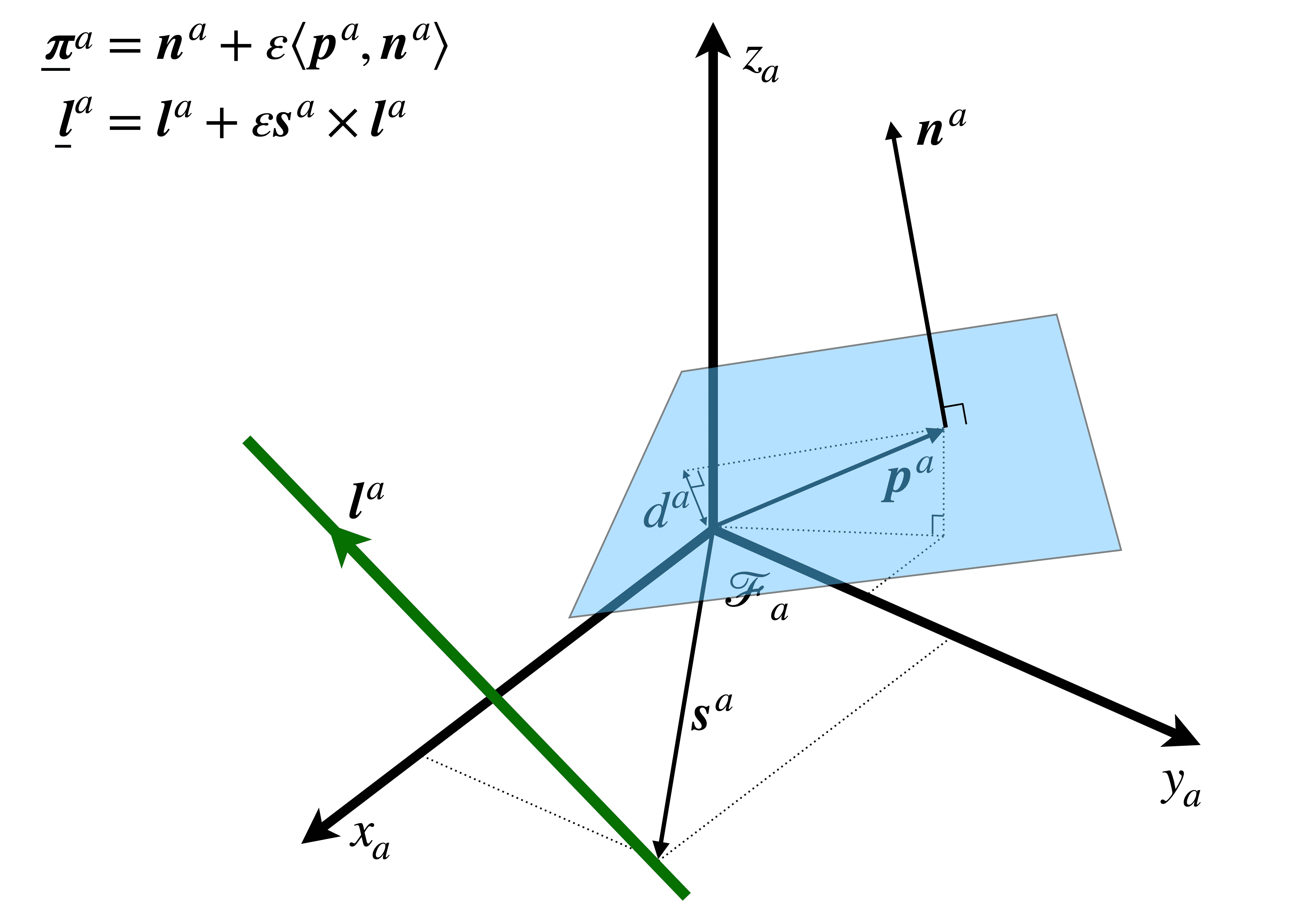
Several geometrical primitives, such as points, planes, and lines are represented as elements of the dual quaternion algebra [8], which is particularly useful when incorporating geometric constraints into robot motion controllers. For instance, a plane expressed in a frame $\mathcal{F}_{a}$ is given by $\underline{\boldsymbol{\pi}}^{a}=\boldsymbol{n}^{a}+\varepsilon d^{a}$, where $\boldsymbol{n}^{a}=n_{x}\hat{\imath}+n_{y}\hat{\jmath}+n_{z}\hat{k}$ is the normal to the plane and $d^{a}=\langle\boldsymbol{p}^{a},\boldsymbol{n}^{a}\rangle$ is the signed distance between the plane and the origin of $\mathcal{F}_{a}$, and $\boldsymbol{p}^{a}$ is an arbitrary point on the plane, as illustrated in Fig. 5.

Figure 5: Two geometric primitives represented by elements of the dual quaternion algebra: (a) the blue plane $\underline{\boldsymbol{\pi}}^{a}$, represented by the normal $\boldsymbol{n}^{a}$ and the distance to the origin $d^{a}=\langle\boldsymbol{p}^{a},\boldsymbol{n}^{a}\rangle$, where $\boldsymbol{p}^{a}$ is an arbitrary point on the plane; (b) and the green line $\underline{\boldsymbol{l}}^{a}$, represented by the direction $\boldsymbol{l}^{a}$ and the moment $\boldsymbol{s}^{a}\times\boldsymbol{l}^{a}$, where $\boldsymbol{s}^{a}$ is an arbitrary point on the line.

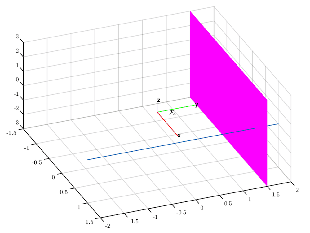
Therefore, the plane $\underline{\boldsymbol{\pi}}^{a}=\hat{\jmath}+\varepsilon 1.5$ (i.e., a plane whose normal is parallel to the $y$-axis and whose distance from $\mathcal{F}_{a}$ is 1.5 m) is defined in DQ Robotics as

⬇

plane_a = j_ + E_ * 1.5;

Analogously, a line in $\mathcal{F}_{a}$, with direction given by $\boldsymbol{l}^{a}=l_{x}\hat{\imath}+l_{y}\hat{\jmath}+l_{z}\hat{k}$ and passing through point $\boldsymbol{s}^{a}=p_{x}\hat{\imath}+p_{y}\hat{\jmath}+p_{z}\hat{k}$, is represented in dual quaternion algebra as $\underline{\boldsymbol{l}}^{a}=\boldsymbol{l}^{a}+\varepsilon\boldsymbol{s}^{a}\times\boldsymbol{l}^{a}$, as illustrated in Fig. 5. Therefore, a line parallel to the $y$-axis passing through point $\boldsymbol{s}^{a}=\hat{\imath}$ (i.e., with coordinates $\left(1,0,0\right)$) is defined in DQ Robotics as

⬇

line_a = j_ + E_ * cross(i_,j_);

In MATLAB, the plot functions are available for frames, planes, and lines:

⬇

plot(DQ(1),’name’,␣’$\mathcal{F}_a$’);

plot(plane_a,␣’plane’,␣20,␣’color’,␣’magenta’);

plot(line_a,␣’line’,␣5);

The result is shown in Fig. 6.

Figure 6: MATLAB plot: reference frame $\mathcal{F}_{a}$; line $\underline{\boldsymbol{l}}^{a}=\hat{\jmath}+\varepsilon(\hat{\imath}\times\hat{\jmath})$ parallel to the $y$-axis and passing through point $(1,0,0)$; and plane $\underline{\boldsymbol{\pi}}^{a}=\hat{\jmath}+\varepsilon 1.5$ with normal parallel to the $y$-axis and whose distance from the origin of $\mathcal{F}_{a}$ is 1.5 m.

The library implements the utility class DQ_Geometry, which provides methods for geometric calculations between primitives, such as distances. Jacobians relating the robot joint velocities to primitives attached to the end-effector are available in the DQ_Kinematics class, such as line_jacobian() and plane_jacobian(). In addition, DQ_Kinematics contains several Jacobians that relate the time derivative of the distance between two primitives (e.g., plane_to_point_distance_jacobian()) which are grouped in the UML class diagram of Fig. 4 as prim_dist_jacobian().

V Robot motion control

Several advantages make dual quaternion algebra attractive when designing controllers. On the one hand, unit dual quaternions are easily mapped into a vector structure. The vector structure is particularly convenient in pose control as there is no need to use intermediate mappings nor extract parameters from the dual quaternion. On the other hand, the position is easily extracted from the HTM, but to obtain the orientation one usually has to extract the rotation angle and the rotation axis from the rotation matrix. This extraction introduces representational singularities when the rotation angle equals zero. Furthermore, when designing constrained controllers based on geometrical constraints, one has to represent several geometrical primitives in different coordinate systems and in different locations. Dual quaternion algebra is particularly useful in this case because several relevant geometrical primitives are easily represented as dual quaternions, as shown in Section IV.

Users can implement their own controllers in DQ Robotics. For instance, suppose that the desired end-effector pose is given by Listing 1 and the initial robot configuration and controller parameters are given in Listing 2.

Listing 2: Parameters for a simple kinematic controller.

⬇

q = [0, 0.3770, 0.1257, -0.5655, 0, 0, 0]’;

T␣=␣0.001;␣␣␣␣␣%␣sampling␣time

gain␣=␣10;␣␣␣␣␣%␣controller␣gain

A classic controller based on an Euclidean error function and the Jacobian pseudo-inverse can be implemented in MATLAB as shown in Listing 3.

Listing 3: Kinematic controller based on the Jacobian pseudoinverse.

⬇

e = ones(8,1); % initialize the error vector

while norm(e) > 0.001

J = lwr4.pose_jacobian(q);

x = lwr4.fkm(q);

e = vec8(x-xd);

u = -pinv(J)*gain*e;

q = q + T*u;

end

In Listing 3, when executing the controller on a real robot, the control input u is usually sent directly to the robot.

There are several kinematic controllers included in DQ Robotics, including the one in Listing 3. The class hierarchy for the kinematic controllers is summarized by the simplified UML diagram in Fig. 7. All kinematic controller classes inherit from the abstract superclass DQ_KinematicController, and their main methods are detailed in Table III.

Figure 7: Simplified UML class diagram of the robot kinematic controller classes with the main methods that are available in C++, Python and MATLAB.

TABLE III: Main methods of class DQ_KinematicController and its main subclasses.

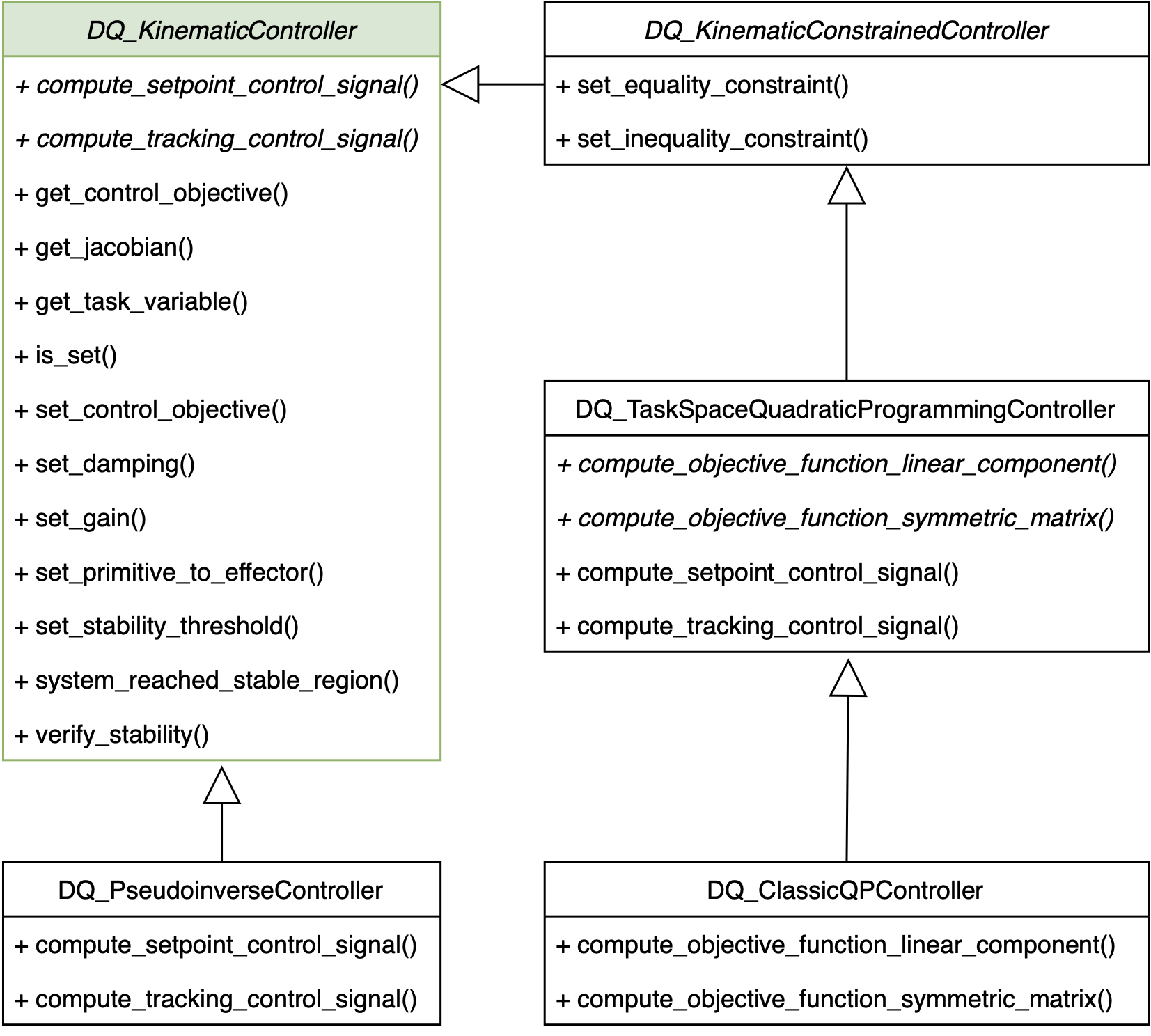
DQ_KinematicController
compute_setpoint_control_signal	Compute the control input to regulate to a set-point.
compute_tracking_control_signal	Compute the control input to track a trajectory.
get_control_objective	Return the control objective.
get_jacobian	Return the correct Jacobian based on the control objective.
get_task_variable	Return the task variable based on the control objective.
is_set	Verify if the controller is set and ready to be used.
set_control_objective	Set the control objective using predefined goals in ControlObjective.
set_damping	Set the damping to prevent instabilities near singular configurations.
set_gain	Set the controller gain.
set_primitive_to_effector	Attach primitive (e.g., plane, line, point) to the end-effector.
set_stability_threshold	Set the threshold that determines if a stable region has been reached.
system_reached_stable_region	Return true if the trajectories of the closed-loop system have reached a stable region (i.e., a positive invariant set), false otherwise.
verify_stability	Verify if the closed-loop region has reached a stable region.
DQ_PseudoinverseSetpointController
compute_tracking_control_signal	Given the task error $\tilde{\boldsymbol{x}}=\boldsymbol{x}-\boldsymbol{x}_{d}\in\mathbb{R}^{n}$, and the feedforward term $\dot{\boldsymbol{x}}_{d}$, compute the control signal $\boldsymbol{u}=\boldsymbol{J}^{+}\left(-\lambda\tilde{\boldsymbol{x}}+\dot{\boldsymbol{x}}_{d}\right)$, where $\boldsymbol{J}^{+}$ is the pseudoinverse of the task Jacobian $\boldsymbol{J}$ and $\lambda$ is the controller gain.
DQ_KinematicConstrainedController
set_equality_constraint	Add equality constraints of type $\boldsymbol{B}\dot{\boldsymbol{q}}=\boldsymbol{b}$, where $\dot{\boldsymbol{q}}\in\mathbb{R}^{n}$ is the vector of joint velocities, $\boldsymbol{b}\in\mathbb{R}^{m}$ is the vector of equality constraints and $\boldsymbol{B}\in\mathbb{R}^{m\times n}$.
set_inequality_constraint	Add inequality constraints of type $\boldsymbol{A}\dot{\boldsymbol{q}}\preceq\boldsymbol{a}$, where $\dot{\boldsymbol{q}}\in\mathbb{R}^{n}$ is the vector of joint velocities, $\boldsymbol{a}\in\mathbb{R}^{m}$ is the vector of inequality constraints and $\boldsymbol{A}\in\mathbb{R}^{m\times n}$.
DQ_TaskspaceQuadraticProgrammingController
compute_objective_function_linear_component	Compute the vector $\boldsymbol{h}$ used in the objective function $(1/2)\dot{\boldsymbol{q}}^{T}\boldsymbol{H}\dot{\boldsymbol{q}}+\boldsymbol{h}^{T}\dot{\boldsymbol{q}}$.
compute_objective_function_symmetric_matrix	Compute the matrix $\boldsymbol{H}$ used in the objective function $(1/2)\dot{\boldsymbol{q}}^{T}\boldsymbol{H}\dot{\boldsymbol{q}}+\boldsymbol{h}^{T}\dot{\boldsymbol{q}}$.
compute_tracking_control_signal	Given the task error $\tilde{\boldsymbol{x}}=\boldsymbol{x}-\boldsymbol{x}_{d}\in\mathbb{R}^{n}$, compute the control signal given by $\boldsymbol{u}\in\arg\min_{\dot{\boldsymbol{q}}}(1/2)\dot{\boldsymbol{q}}^{T}\boldsymbol{H}\dot{\boldsymbol{q}}+\boldsymbol{h}^{T}\dot{\boldsymbol{q}}$ subject to $\boldsymbol{A}\dot{\boldsymbol{q}}\preceq\boldsymbol{a}$ and $\boldsymbol{B}\dot{\boldsymbol{q}}=\boldsymbol{b}$.
DQ_ClassicQPController
compute_objective_function_linear_component	Compute the vector $\boldsymbol{h}$ used in $(1/2)\dot{\boldsymbol{q}}^{T}\boldsymbol{H}\dot{\boldsymbol{q}}+\boldsymbol{h}^{T}\dot{\boldsymbol{q}}=\left\|\boldsymbol{J}\dot{\boldsymbol{q}}+\lambda\tilde{\boldsymbol{x}}-\dot{\boldsymbol{x}}_{d}\right\|_{2}^{2}$.
compute_objective_function_symmetric_matrix	Compute the matrix $\boldsymbol{H}$ used in $(1/2)\dot{\boldsymbol{q}}^{T}\boldsymbol{H}\dot{\boldsymbol{q}}+\boldsymbol{h}^{T}\dot{\boldsymbol{q}}=\left\|\boldsymbol{J}\dot{\boldsymbol{q}}+\lambda\tilde{\boldsymbol{x}}-\dot{\boldsymbol{x}}_{d}\right\|_{2}^{2}$.

*Abstract methods are written in italics and concrete methods are written in upright. In all concrete classes, the method compute_setpoint_control_signal() does not include the feedforward term in the method parameters and is equivalent to the method compute_tracking_control_signal with $\dot{\boldsymbol{x}}_{d}=\boldsymbol{0}$. Therefore, they are omitted for the sake of conciseness.

The DQ_KinematicController subclasses are focused on the control structure, not on particular geometrical tasks. The same subclass can be used regardless if the goal is to control the end-effector pose, position, orientation, etc. In order to distinguish between task objectives, it suffices to use

⬇

controller.set_control_objective(GOAL)

where GOAL is an object from the enumeration class ControlObjective, which currently provides the following enumeration members: Distance, DistanceToPlane, Line, Plane, Pose, Rotation, and Translation. Therefore, the implementation in Listing 3 can be rewritten using the DQ_PseudoinverseController class as

Listing 4: Controller based on the DQ_PseudoinverseController class.

⬇

control = DQ_PseudoinverseController(lwr4);

control.set_control_objective(ControlObjective.Pose);

control.set_gain(gain);

control.set_stability_threshold(0.0001);

while ~control.system_reached_stable_region()

u = control.compute_setpoint_control_signal(q,vec8(xd));

q = q + T*u;

end

Furthermore, if the geometric task objective changes, the DQ_KinematicController subclass is responsible for calculating the appropriate forward kinematics and the corresponding Jacobian. For instance, if a line is attached to the end-effector and the goal is to align it with a line in the workspace, then it suffices to replace the second line of Listing 4 by

⬇

control.set_primitive_to_effector(line);

control.set_control_objective(ControlObjective.Line);

where line is a dual quaternion corresponding to a line passing through the origin of the end-effector frame.

Furthermore, since any subclass of DQ_KinematicController provides the methods used in Listing 4, changing the controller is a matter of changing just one line of code, namely the first one in Listing 4.

VI Interface with ROS

The Robot Operating System (ROS) [9] is widely used by the robotics community. After the one-line installation described in Section VIII, the Python version of the DQ Robotics library can be imported in any Python script in the system; therefore, it is compatible with ROS out-of-the-box. MATLAB also has an interface with ROS.

For C++ code, in its most recent versions, ROS uses the catkin_build environment, which itself depends on CMAKE. Given that DQ Robotics C++ is installed as a system library in Ubuntu, as shown in Section VIII, ROS users can readily have access to the library as they would to any other system library with a proper CMAKE configuration. After installation, the C++ version of the library can be linked with

⬇

target_link_libraries(my_binary dqrobotics)

for a given binary called my_binary.

VII Interface with V-REP

DQ Robotics provides a simple interface to V-REP [10], enabling users to develop complex simulations without having to delve into the V-REP documentation. The V-REP interface comes bundled with the MATLAB and Python versions of the library. The C++ version of our V-REP interface comes as a separate package and the following CMAKE directive will link the required shared object

⬇

target_link_libraries(my_binary

dqrobotics

dqrobotics-vrep-interface)

for a given my_binary.

The available methods are shown in Table IV.

TABLE IV: VrepInterface.

connect	Connect to a V-REP Remote API Server.
disconnect	Disconnect from currently connected server.
disconnect_all	Flush all Remote API connections.
start_simulation	Start V-REP simulation.
stop_simulation	Stop V-REP simulation.
get_object_translation	Get object translation as a pure quaternion.
set_object_translation	Set object translation with a pure quaternion.
get_object_rotation	Get object rotation as a unit quaternion.
set_object_rotation	Set object rotation with a unit quaternion.
get_object_pose	Get object pose as a unit dual quaternion.
set_object_pose	Set object pose with a unit dual quaternion.
set_joint_positions	Set the joint positions of a manipulator robot.
set_joint_target_positions	Set the joint target positions of a manipulator robot.
get_joint_positions	Get the joint positions of a manipulator robot.

To start the communication with V-REP using its remote API, only two methods are necessary:

⬇

vi = DQ_VrepInterface;

vi.connect(’127.0.0.1’,19997);

vi.start_simulation();

The method start_simulation starts the V-REP simulation with the default asynchronous mode and the recommended 5 ms communication thread cycle.

Since each robot joint in V-REP is associated with a name, it is convenient to encapsulate this information inside the robot class. Therefore, classes implementing robots that use the V-REP interface must be a subclass of DQ_VrepRobot to provide the methods send_q_to_vrep, and get_q_from_vrep, which are used to send the desired robot configuration vector to V-REP and get the current robot configuration vector from V-REP, respectively.

Objects poses in a V-REP scene can be retrieved or set by using the methods get_object_pose and set_object_pose, respectively, which are useful when designing motion planners or controllers that take into account the constraints imposed by obstacles. Finally, in order to end the V-REP simulation it suffices to use two methods:

⬇

vi.stop_simulation();

vi.disconnect();

VII-A A more complete example

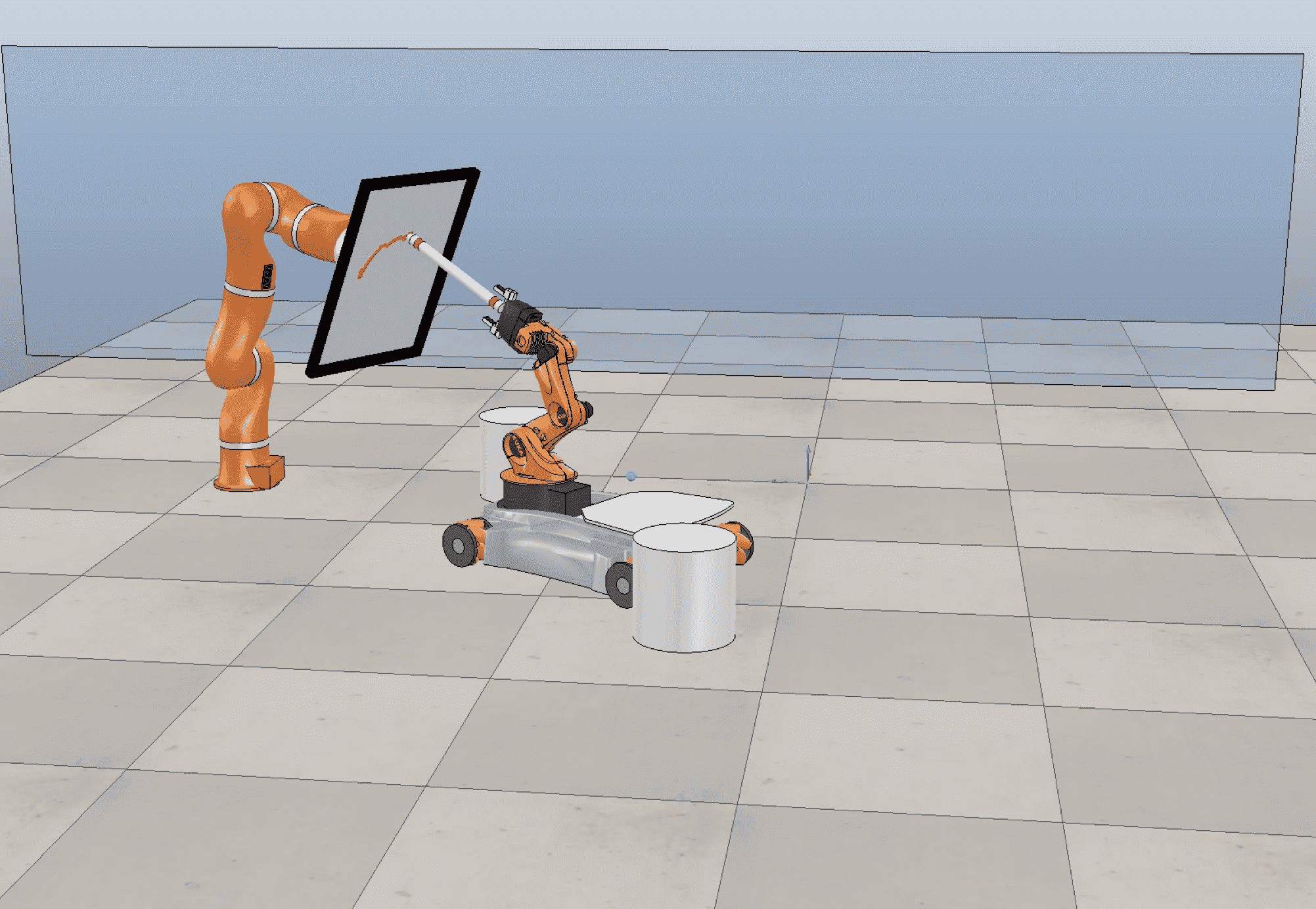
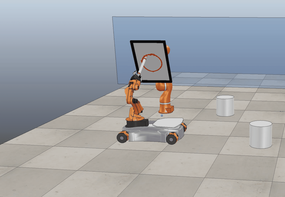
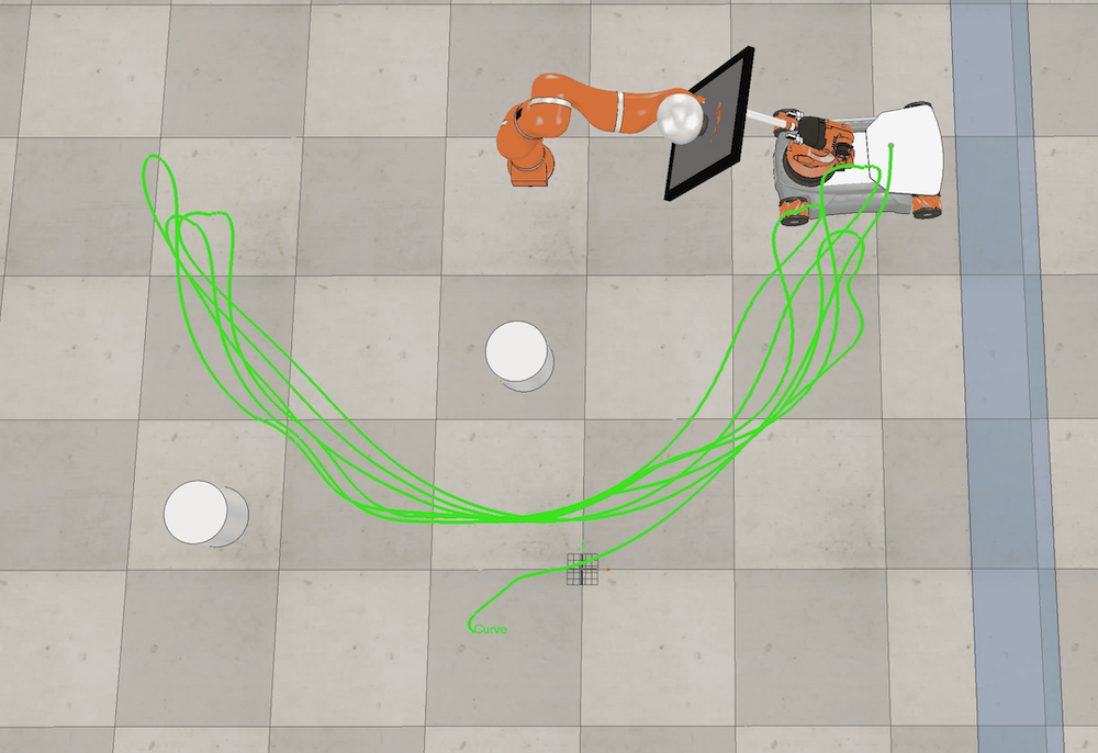
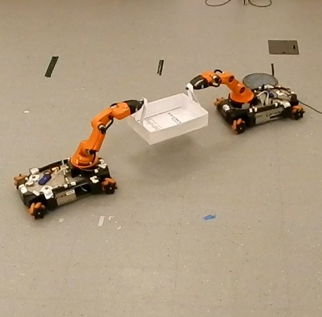
To better highlight how DQ Robotics can be used with V-REP, in this example, a KUKA LWR4 manipulator robot interacts with a KUKA YouBot mobile manipulator in a workspace containing three obstacles, namely two cylinders and a plane, as shown in Fig. 8.

Figure 8: A more complete example. The reference frame is given by $\mathcal{F}$, the time-varying frame $\mathcal{F}_{c}$ is used to indicate where the circle must be drawn in the whiteboard, and $\mathcal{F}_{mm}$ is the end-effector frame of the mobile manipulator. Obstacles are represented as geometrical primitives: the wall is represented by the plane $\underline{\boldsymbol{\pi}}=\boldsymbol{n}_{\underline{\boldsymbol{\pi}}}+\varepsilon\langle\boldsymbol{p}_{\underline{\boldsymbol{\pi}}},\boldsymbol{n}_{\underline{\boldsymbol{\pi}}}\rangle$, where $\boldsymbol{p}_{\underline{\boldsymbol{\pi}}}$ is an arbitrary point on the plane and $\boldsymbol{n}_{\underline{\boldsymbol{\pi}}}$ is the plane normal, and the two cylindrical obstacles are represented by $\left(\underline{\boldsymbol{l}}_{1},R_{1}\right)$ and $\left(\underline{\boldsymbol{l}}_{2},R_{2}\right)$, where $\underline{\boldsymbol{l}}_{i}=\boldsymbol{l}_{i}+\varepsilon\boldsymbol{p}_{i}\times\boldsymbol{l}_{i}$ is the ith cylinder centerline and $R_{i}$ is the corresponding cylinder radius with $i\in\{1,2\}$. Furthermore, $\boldsymbol{l}_{i}$ is the line direction and $\boldsymbol{p}_{i}$ is an arbitrary point on the ith line. To prevent collisions between the robot and the obstacles, the robot is represented by a circle given by $\left(\boldsymbol{p}_{3},R_{3}\right)$, where $\boldsymbol{p}_{3}$ and $R_{3}$ are the center and radius of the circle, respectively.

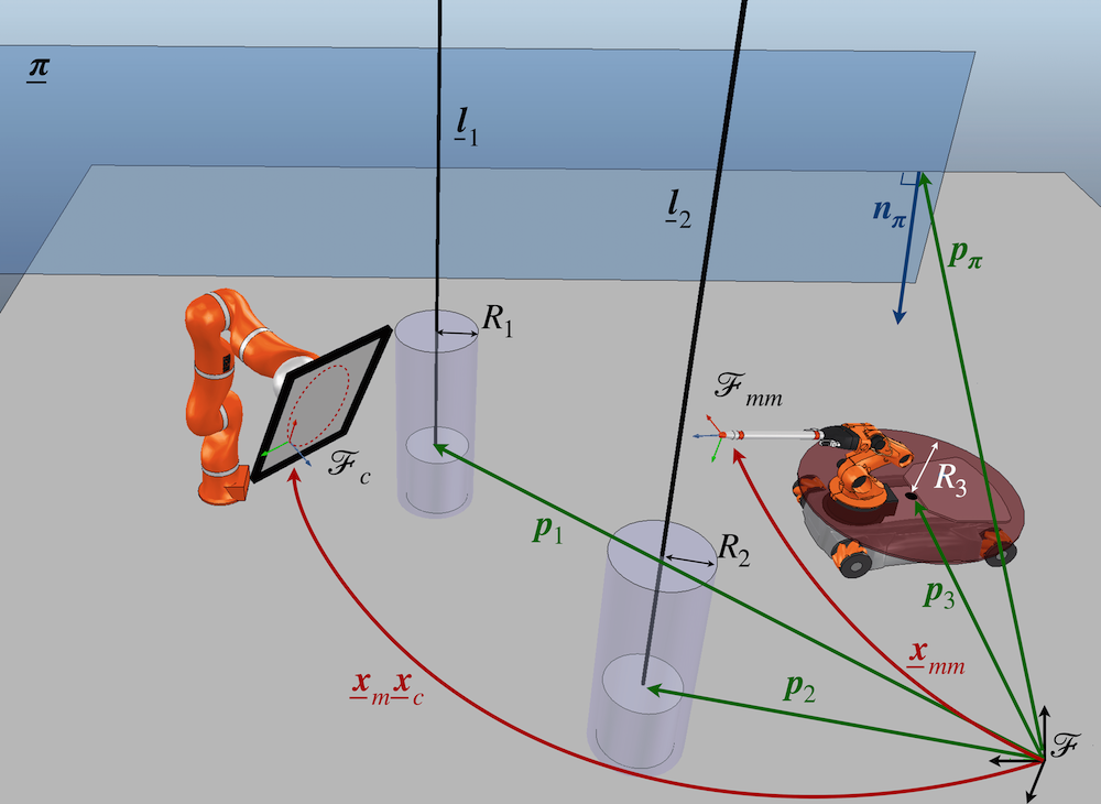
The manipulator robot holds a whiteboard and uses a pseudo-inverse-based controller with a feedforward term to track a trajectory, given by $\underline{\boldsymbol{x}}_{m}(t)=\boldsymbol{r}_{m}(t)\underline{\boldsymbol{x}}_{m}(0)\boldsymbol{p}_{m}(t)$, where $\boldsymbol{r}_{m}=\cos(\phi(t)/2)+\hat{k}\sin(\phi(t)/2)$ with $\phi(t)=(\pi/2)\sin(\omega_{n}t)$, and $\boldsymbol{p}=1+(1/2)\varepsilon d_{z}\cos(\omega_{d}t)\hat{k}$. Viewed from the top, the whiteboard will follow a semi-circular path with a radial oscillation at a frequency of $\omega_{d}\,\mathrm{rad/s}$ and amplitude $d_{z}\,\mathrm{m}$, and an oscillation around the vertical axis at a frequency of $\omega_{n}\,\mathrm{rad/s}$. The mobile manipulator holds a felt pen and follows the manipulator trajectory while drawing a circle on the whiteboard. The mobile manipulator desired end-effector trajectory is given by $\underline{\boldsymbol{x}}_{mm}(t)=\underline{\boldsymbol{x}}_{m}(t)\underline{\boldsymbol{x}}_{c}\hat{\jmath}$, where $\underline{\boldsymbol{x}}_{c}=1+(1/2)\varepsilon 0.015\hat{k}$ is a constant displacement of $1.5\mathrm{cm}$ along the $z$-axis to account for the whiteboard width and $\hat{\jmath}=\cos(\pi/2)+\hat{\jmath}\sin(\pi/2)$ is a rotation of $\pi$ around the $y$-axis so that both end-effectors have their $z$-axis pointing to opposite directions. To prevent collision with obstacles it uses a constrained controller, in which for each obstacle we use a differential inequality to ensure that the robot will approach it, in the worst case, with an exponential velocity decrease. For each obstacle, we define a distance metric ${\tilde{d}\left(t\right)\triangleq d\left(t\right)-d_{\mathrm{safe}}}$, where $d_{\mathrm{safe}}\in\left[0,\infty\right)$ is an arbitrary constant safe distance, and the following inequalities must hold for all $t$ :

$$\dot{\tilde{d}}\left(t\right)\geq- \eta_{d}\tilde{d}\left(t\right)\Longleftrightarrow-\boldsymbol{J}_{d}\dot{\boldsymbol{q}}\leq\eta_{d}\tilde{d}\left(t\right),$$ (2)

where $\eta_{d}\in[0,\infty)$ is used to adjust the approach velocity and $\boldsymbol{J}_{d}$ is the distance Jacobian related to the obstacle [11]. The lower is $\eta_{d}$, the lower is the allowed approach velocity.

In the case of our example, to prevent collisions between the robot and the wall, we let $d_{\mathrm{safe}}\triangleq R_{3}$ (see Fig. 8) such that $\tilde{d}\left(t\right)=0\iff d\left(t\right)=R_{3}$, and the distance function is defined as the distance between $\boldsymbol{p}_{3}$, which is the center of the circle enclosing the robot, and the wall plane $\underline{\boldsymbol{\pi}}$. Analogously, to prevent collisions between the robot and the static cylinders, we use one inequality such as (2) for each cylinder, where $d_{\mathrm{safe}}\triangleq R_{i}+R_{3}$ and $d(t)$ is defined as the distance between $\boldsymbol{p}_{3}$ and the lines $\underline{\boldsymbol{l}}_{i}$, for $i\in\{1,2\}$. Although those distance functions and corresponding Jacobians can be computed by using the classes DQ_Geometry and DQ_Kinematics, respectively, details of how they are obtained using dual quaternion algebra are presented in [11].

Whenever the felt-tip is sufficiently close to the whiteboard, it starts to draw a circle. Figs. 9a and 9b show that the mobile manipulator successfully draws the circle, although there are some small imperfections as the obstacle avoidance is a hard constraint that is always respected at the expense of worse trajectory tracking. Last, Fig. 9c shows the mobile manipulator trajectory, which is always adapted to prevent collisions with the cylinders and the wall.

(a) Circle partially drawn at $t=36\mathrm{s}$.

(b) Circle completely drawn at $t=170\mathrm{s}$.

(c) Top view showing the mobile manipulator trajectory.

Figure 9: Manipulator robot interacting with a mobile manipulator in a workspace with two cylindrical obstacles and a wall. The parameters for the trajectory generation were $\omega_{n}=0.1$, $\omega_{d}=0.5$ and $d_{z}=0.1$.

The main MATLAB code is shown in Listing 5. For the sake of conciseness, the functions compute_lwr4_reference and compute_youbot_reference, which calculate the aforementioned end-effector trajectories, are omitted. The same applies for get_plane_from_vrep and get_line_from_vrep, which get information about the location of the corresponding geometric primitives in V-REP, and compute_constraints, which calculates constraints such as (2) for each obstacle in the scene. The original source code used in this example is available as supplementary material. For a more up-to-date version, refer to https://github.com/dqrobotics/matlab-examples.

Listing 5: Main MATLAB code for the simulation.

⬇

sampling_time = 0.05;

total_time = 200;

for t=0:sampling_time:total_time

%% Get obstacles from V-REP

plane = get_plane_from_vrep(vi,’ObstaclePlane’,DQ.k);

cylinder1␣=␣get_line_from_vrep(vi,’ObstacleCylinder1’,DQ.k);

cylinder2␣=␣get_line_from_vrep(vi,’ObstacleCylinder2’,DQ.k);

%%␣Set␣references␣for␣both␣robots

[lwr4_xd,␣lwr4_ff]␣=␣compute_lwr4_reference(lwr4,...

␣␣␣␣simulation_parameters,␣lwr4_x0,␣t);

[youbot_xd,␣youbot_ff]␣=␣compute_youbot_reference(...

␣␣␣␣youbot_control,␣lwr4_xd,␣lwr4_ff);

%%␣Compute␣the␣control␣input␣for␣the␣manipulator

lwr4_u␣=␣lwr4_controller.compute_tracking_control_signal(...

␣␣␣␣lwr4_q,␣vec8(lwr4_xd),vec8(lwr4_ff));

%%␣Compute␣constrained␣control␣input␣for␣the␣youbot

[Jconstraint,␣bconstraint]␣=␣compute_constraints(youbot,␣...

␣␣␣␣youbot_q,␣plane,cylinder1,cylinder2);

youbot_control.set_inequality_constraint(-Jconstraint,...

␣␣␣␣1*bconstraint);

youbot_u=␣youbot_control.compute_tracking_control_signal(...

␣␣␣␣youbot_q,␣vec8(youbot_xd),␣vec8(youbot_ff));

%␣Since␣we␣are␣using␣V-REP␣just␣for␣visualization,␣integrate

%␣the␣control␣signal␣to␣update␣the␣robots␣configurations

lwr4_q␣=␣lwr4_q␣+␣sampling_time*lwr4_u;

youbot_q␣=␣youbot_q␣+␣sampling_time*youbot_u;

%%␣Send␣desired␣values␣to␣V-REP

lwr4_vreprobot.send_q_to_vrep(lwr4_q);

youbot_vreprobot.send_q_to_vrep(youbot_q);

end

VIII Development infrastructure

Aiming at the scalability of the DQ Robotics library and taking advantage of the familiarity that current developers have with Git and Github, we opted to also use those services.

End-users are agnostic to these infrastructural decisions. For them, usage, performance, and installation of the library matter the most. The usage of the library has been simplified by relying on a programming syntax similar to the mathematical description and being attentive to proper object-oriented programming practices. Furthermore, good performance is achieved by careful optimization of the library and by the C++ implementation.

The ease of installation has been addressed in language/platform specific ways that we document in details on the DQ Robotics’ Read the Docs.

For MATLAB, DQ Robotics is distributed as a Toolbox that can be installed by the end-user in any of the MATLAB-compatible operating systems.

For C++, we officially focus on Ubuntu long-term service (LTS) distributions, in a similar way to the most recent distributions of ROS and other large open-source libraries such as TensorFlow. For any Ubuntu LTS distribution that has not reached its end-of-life, the user can install the C++ version of the library with the following three commands

⬇

sudo add-apt-repository ppa:dqrobotics-dev/release

sudo apt-get update

sudo apt-get install libdqrobotics

made available via our release Personal Package Archive (PPA), in which we store the latest stable versions of the library. Interfaces between DQ Robotics and other libraries also reside in the same PPA. For example, after adding the PPA, the user can install the V-REP interface with the following command

⬇

sudo apt-get install libdqrobotics-interface-vrep

The PPA guarantees that the user can reliably install the package in their system as the PPA only stores packages that compiled successfully. Support for other operating systems will be driven by user interest, but should not be a big challenge for most systems since we are using only CMAKE and Eigen3 as project dependencies, both of which are widely supported.

Lastly, the Python version of DQ Robotics is made available through a Pybind11-based Python wrapper of the C++ library. This has three main advantages. First, there is no need to redevelop and maintain versions of the libraries in different programming languages, which is highly demanding. Second, unit-testing code written in Python, which is easier to write and maintain, automatically validates the C++ library as well. Third, we can have Python’s ease-of-use with C++’s performance for each function. Although there is a computational overhead when using the Python bindings (in contrast with directly using the C++ code), it is much lower than a native Python implementation. A simple example of this can be seen in Table V, in which we compare the average required time for dual quaternion multiplications in the same machine.

TABLE V: Computational time of dual-quaternion multiplications.

	Mean [$\mu$s]	Standard Deviation [$\mu$s]
C++ (gcc 5.4.0)	0.22	0.0149
MATLAB R2019a	8.94	0.1223
Python 3.5.2 Bindings	0.82	0.0242
Python 3.5.2 Native	31.42	0.1646

*Mean and standard deviation of the required time for one dual-quaternion multiplication. This was calculated from a thousand sets of a thousand executions on the same Intel Core i9 9900K Ubuntu 16.04 x64 system and excludes the time required to generate the random dual quaternions.

An Ubuntu LTS user can install the Python3 version of DQ Robotics from the Python Package Index (PyPI) with a single line of code

⬇

python3 -m pip install --user dqrobotics

Lastly, the PyPI package is continuously built from source using TravisCI, so that the code is properly compiled and tested before being distributed to our users.

IX Applications and comparison with other packages and libraries

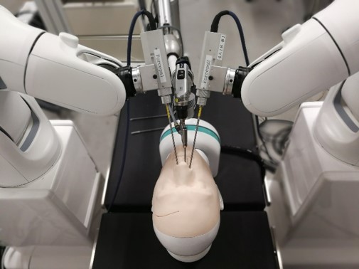
DQ Robotics has been used for more than nine years to model and control different robots in applications such as bimanual surgical robots in constrained workspaces (Fig. 10a), whole-body control of humanoid robots (Fig. 10b), and the decentralized formation control of mobile manipulators (Fig. 10c).

(a) The bimanual surgical robot SmartArm [12].

(b) Whole-body control of a humanoid robot [13].

(c) Cooperative mobile manipulators[14].

Figure 10: Examples of different applications of DQ Robotics.

The main difference from other packages and libraries is that DQ Robotics implements dual quaternion algebra in a close way to the mathematical notation. Furthermore, all supported languages, namely Python, MATLAB, and C++, use the same convention and style and it is straightforward to port code in one language to other supported languages. To enable that, we avoid using features that are not available in all three languages, unless that would lead to poor-quality code. From the user point-of-view, the advantage of such approach is that users can prototype their ideas on MATLAB using the convenient plot system, then easily translate the code to C++ and deploy it on a real robotic platform. The Python version of the library is somewhere between MATLAB and C++, being suitable for prototyping and also for deployment on real applications because C++ runs under the hood.

In terms of target audience, the MATLAB version of DQ Robotics has some overlap with Peter Corke’s Robotics Toolbox [15], most notably in terms of their use for education and learning. On the one hand, earlier versions were greatly inspired by Peter Corke’s Robotics Toolbox, most notably the plot system, which is particularly useful when teaching robotics. On the other hand, DQ Robotics is entirely based on general dual quaternion algebra whereas Robotics Toolbox uses classic representations for robot modeling, although it does offer support for unit quaternions. Moreover, other functionalities of Peter Corke’s Robotics Toolbox such as path planning, localization, and mapping are not available in DQ Robotics as of now. However, some functionalities of Peter Corke’s Robotics Toolbox are now available in toolboxes distributed by MathWorks, such as the Image Processing Toolbox and the Robotics System Toolbox, which are, in principle, compatible with DQ Robotics.

Another MATLAB toolbox [7] focuses on the application of unit dual quaternions to the neuroscience domain and presents basic kinematic modeling of serial mechanisms. In addition to having many fewer functionalities than DQ Robotics, it uses procedural programming, which makes the code quite different from the notation used on paper.

A major contrast between DQ Robotics and Peter Corke’s and Leclercq’s MATLAB toolboxes is that DQ Robotics has Python and C++ versions with identical APIs, as far as the programming languages permit. This increases the number of possible users and considerably reduces the time required to go from prototyping to deployment. Moreover, this makes DQ Robotics compatible with powerful libraries available in Python such as SciPy and scikit-learn. In addition, both Python and C++ versions of the library can be readily used alongside ROS, which is the current standard of shareable code in the robotics community. Lastly, a modern development infrastructure, not available in other existing libraries, makes the library scalable and easier to maintain and extend.

X Conclusions

This paper presented DQ Robotics, a comprehensive computational library for robot modeling and control using dual quaternion algebra. It has the unique feature of using a notation very close to the mathematical description and supporting three different programming languages, namely MATLAB, Python, and C++, while using very similar conventions among them, making it very easy to switch between languages and thus shortening the development time from prototyping to the implementation on actual robots. The library currently supports serial manipulator robots, cooperative systems such as two-arm robots, mobile manipulators and even branched mechanisms such as humanoids. Robot models are generated automatically from simple geometrical parameters, such as the Denavit-Hartenberg parameters. In addition, robots can be easily combined to yield more complex ones while the corresponding forward kinematics and differential kinematics are also computed automatically and analytically at execution time. The library also offers a rich set of motion controllers and it is very simple to implement new ones. Although it does not offer dynamics modeling yet, it can be easily integrated to existing libraries for that purpose. However, robot dynamics modeling using dual quaternion algebra is currently under development and will be integrated into the library as soon as it becomes mature. Rather than being a competitor to existing libraries, DQ Robotics aims at complementing them and helping in the popularization of dual quaternion algebra in the robotics domain.

References

- [1] O. Bottema and B. Roth, Theoretical kinematics. North-Holland Publishing Company, 1979, vol. 24.
- [2] J. McCarthy, Introduction to theoretical kinematics, 1st ed. The MIT Press, 1990.
- [3] B. V. Adorno, “Two-arm Manipulation: From Manipulators to Enhanced Human-Robot Collaboration [Contribution à la manipulation à deux bras : des manipulateurs à la collaboration homme-robot],” PhD Dissertation, Université Montpellier 2, 2011. [Online]. Available: https://tel.archives-ouvertes.fr/tel-00641678/
- [4] M. W. Spong and M. Vidyasagar, Robot dynamics and control. John Wiley & Sons, 2008.
- [5] B. Siciliano, L. Sciavicco, L. Villani, and G. Oriolo, Robotics: modelling, planning and control. Springer Science & Business Media, 2010.
- [6] B. Siciliano and O. Khatib, Springer handbook of robotics. Springer, 2016.
- [7] G. Leclercq, P. Lefèvre, and G. Blohm, “3D kinematics using dual quaternions: theory and applications in neuroscience,” Frontiers in Behavioral Neuroscience, vol. 7, no. February, p. 7, jan 2013. [Online]. Available: http://www.ncbi.nlm.nih.gov/pubmed/23443667http://journal.frontiersin.org/article/10.3389/fnbeh.2013.00007/abstract
- [8] B. V. Adorno, “Robot Kinematic Modeling and Control Based on Dual Quaternion Algebra – Part I: Fundamentals,” 2017. [Online]. Available: https://hal.archives-ouvertes.fr/hal-01478225v1
- [9] M. Quigley, K. Conley, B. Gerkey, J. Faust, T. Foote, J. Leibs, R. Wheeler, and A. Y. Ng, “Ros: an open-source robot operating system,” in ICRA workshop on open source software, vol. 3, no. 3.2. Kobe, Japan, 2009, p. 5.
- [10] E. Rohmer, S. P. N. Singh, and M. Freese, “V-REP: A versatile and scalable robot simulation framework,” in 2013 IEEE/RSJ International Conference on Intelligent Robots and Systems. IEEE, nov 2013.
- [11] M. M. Marinho, B. V. Adorno, K. Harada, and M. Mitsuishi, “Dynamic Active Constraints for Surgical Robots Using Vector-Field Inequalities,” IEEE Transactions on Robotics, vol. 35, no. 5, pp. 1166–1185, oct 2019. [Online]. Available: https://ieeexplore.ieee.org/document/8742769/
- [12] M. M. Marinho, K. Harada, A. Morita, and M. Mitsuishi, “Smartarm: Integration and validation of a versatile surgical robotic system for constrained workspaces,” The International Journal of Medical Robotics and Computer Assisted Surgery, (in press) 2019.
- [13] J. J. Quiroz-Omana and B. V. Adorno, “Whole-Body Control With (Self) Collision Avoidance Using Vector Field Inequalities,” IEEE Robotics and Automation Letters, vol. 4, no. 4, pp. 4048–4053, oct 2019. [Online]. Available: https://ieeexplore.ieee.org/document/8763977/
- [14] H. J. Savino, L. C. Pimenta, J. A. Shah, and B. V. Adorno, “Pose consensus based on dual quaternion algebra with application to decentralized formation control of mobile manipulators,” Journal of the Franklin Institute, pp. 1–36, oct 2019. [Online]. Available: https://linkinghub.elsevier.com/retrieve/pii/S0016003219307161
- [15] P. Corke, Robotics, Vision and Control, 2nd ed., ser. Springer Tracts in Advanced Robotics. Springer International Publishing, 2017, vol. 118. [Online]. Available: http://link.springer.com/10.1007/978-3-319-54413-7