Abstract

We analyze the convergence rate of the randomized Newton-like method introduced by Qu et al., (2016) for smooth and convex objectives, which uses random coordinate blocks of a Hessian-over-approximation matrix $\mathbf{M}$ instead of the true Hessian. The convergence analysis of the algorithm is challenging because of its complex dependence on the structure of $\mathbf{M}$. However, we show that when the coordinate blocks are sampled with probability proportional to their determinant, the convergence rate depends solely on the eigenvalue distribution of matrix $\mathbf{M}$, and has an analytically tractable form. To do so, we derive a fundamental new expectation formula for determinantal point processes. We show that determinantal sampling allows us to reason about the optimal subset size of blocks in terms of the spectrum of $\mathbf{M}$. Additionally, we provide a numerical evaluation of our analysis, demonstrating cases where determinantal sampling is superior or on par with uniform sampling.

1 INTRODUCTION

We study unconstrained optimization of the form:

$$\min_{x\in\mathbb{R}^{d}}f(x),$$

where we assume that the function $f:\mathbb{R}^{d}\rightarrow\mathbb{R}$ is smooth, convex, and potentially high dimensional. This problem commonly arises in empirical risk minimization (ERM, see Shalev-Shwartz and Ben-David,, 2014). State-of-the-art approaches for minimization of convex ERM objectives with large numbers of data points include variants of stochastic gradient descent (SGD) such as SVRG (Johnson and Zhang,, 2013), SARAH (Nguyen et al.,, 2017) and a plethora of others. Alternatively, one can approach the ERM problem via a dual formulation, where fast coordinate minimization techniques such as SDCA (Shalev-Shwartz and Zhang,, 2013), or parallel coordinate descent (Richtárik and Takáč,, 2016, 2015) can be applied. This is especially desirable in distributed and parallel environments (Richtárik and Takác,, 2013; Ma et al.,, 2015; Dünner et al.,, 2016). These approaches are closely related to methods that subsample the Hessian (Pilanci and Wainwright,, 2015; Roosta-Khorasani and Mahoney,, 2016, 2016).

We study a block coordinate descent algorithm first introduced by Qu et al., (2016). In each iteration of this algorithm, we sample a block of coordinates and then solve a Newton step on the chosen coordinate subspace. However, in place of the true Hessian, a fixed over-approximation matrix $\mathbf{M}$ is used for the sake of efficiency. The Newton step is computed on a sparsified version of this matrix with all but the selected coordinates set to zero, denoted $\mathbf{M}_{\hat{S}}$ (see Section 1.2 for the complete notation). Originally, Qu et al., (2016) called this method Stochastic Dual Newton Ascent (SDNA), appealing to the fact that it operates in a dual ERM formulation. Later, it was also called a Stochastic Newton method (Mutný and Richtárik,, 2018), while we use the name Randomized Newton Method (RNM) following Gower et al., (2019).

The sampling strategy for the coordinate blocks has a dramatic impact on the convergence rate (Qu and Richtárik,, 2016). Gower and Richtárik, (2015) demonstrate that by optimizing the sampling probabilities one can obtain very significant speedups, however this optimization is a semidefinite program which may be even more challenging than the original optimization problem itself. Even when using a basic sampling strategy (such as uniform), the convergence analysis of RNM is challenging because it hinges on deriving the expected pseudoinverse of $\mathbf{M}_{\hat{S}}$, henceforth denoted $\mathbb{E}[(\mathbf{M}_{\hat{S}})^{+}]$. Prior to this work, no simple closed form expression was known for this quantity.

To overcome this challenge, we focus on a strategy of randomly sampling blocks of coordinates proportionally to the determinant of the corresponding submatrix of $\mathbf{M}$, which we call determinantal sampling. Similar sampling schemes have been analyzed in the context of stochastic optimization before (Zhang et al.,, 2017; Borsos et al.,, 2019). Recently, Rodomanov and Kropotov, (2019) analyzed determinantal sampling for randomized block coordinate descent, however they imposed cardinality constraints on the block size, and as a result were unable to obtain a simple expression for $\mathbb{E}[(\mathbf{M}_{\hat{S}})^{+}]$.

We use determinantal sampling with randomized block size, which allows us to obtain a simple closed form expression for the expected pseudoinverse:

$$\mathbb{E}[(\mathbf{M}_{\hat{S}})^{+}]=(\alpha\mathbf{I}+\mathbf{M})^{-1},$$

where $\alpha$ is a tunable parameter that is used to control the expected block size. With the use of this new expectation formula, we establish novel bounds on the convergence rate of RNM depending on the spectral properties of the over-approximating matrix $\mathbf{M}$. For many instances of the problem, the matrix coincides with the data covariance, and spectral decays of such covariances are well understood (Blanchard et al.,, 2007). This allows us to predict the decay-specific behavior of RNM with determinantal sampling and recommend the optimal block size.

The cost of each iteration of RNM scales cubically with the size of the block due to matrix inversion. Qu et al., (2016) demonstrate numerically that for small blocks the optimization time decreases but at some point it starts to increase again. They surmise that the improvement is obtained only as long as the inversion cost is dominated by the other fixed per-iteration costs such as fetching from memory. However, whether the only possible speedup stems from this has remained unclear. We answer this question for determinantal sampling by deriving the optimal subset size in the case of kernel ridge regression. We show that when the eigenvalue decay is sufficiently rapid, then the gain in convergence rate can dominate the cost of inversion even for larger block sizes.

1.1 Contributions

The main contributions of this paper can be summarized as follows:

• We obtain a novel and remarkably simple expectation formula for determinantal sampling that allows us to derive a simple and closed form expression for the convergence rate of the Randomized Newton Method.

• This allows us to improve the previous bounds on the theoretical speedup of using coordinate blocks of larger sizes. For example, we show that in the case of kernel regression with a covariance operator that has exponentially decreasing spectrum, the theoretical speedup is exponential.

• We take into account the actual per iteration cost, and analyze not only the convergence rate of the algorithm, but also its numerical effort to solve a problem up to some relative precision. This allows us to classify the problems into categories where the optimal block size is one, the full matrix, or somewhere in between.

• We numerically validate the discovered theoretical properties of determinantal sampling, and demonstrate cases when it improves over uniform sampling, and when it performs similarly. If the two perform similarity, our analysis serves as a more interpretable proxy for the convergence analysis of uniform sampling.

1.2 Notation

Let $S$ be a non-empty subset of $[d]:=\{1,2,\dots,d\}$. We let $\mathbf{I}_{:S}$ be the $d\times|S|$ matrix composed of columns $i\in S$ of the $d\times d$ identity matrix $\mathbf{I}$. Note that $\mathbf{I}_{:S}^{\top}\mathbf{I}_{:S}$ is the $|S|\times|S|$ identity matrix. Given an invertible matrix $\mathbf{M}\in\mathbb{R}^{d\times d}$, we can extract its principal $|S|\times|S|$ sub-matrix with the corresponding rows and columns indexed by $S$ via $\mathbf{M}_{SS}\overset{\text{def}}{=}\mathbf{I}_{:S}^{\top}\mathbf{M}\mathbf{I}_{:S}$, and additionally keeping the sub-matrix in its canonical place we can define the following operation,

$$\mathbf{M}_{S}\overset{\text{def}}{=}\mathbf{I}_{:S}\mathbf{M}_{SS}\mathbf{I}_{:S}^{\top}.$$ (1)

Note that $\mathbf{M}_{S}$ is the $n\times n$ matrix obtained from $\mathbf{M}$ by retaining elements $\mathbf{M}_{ij}$ for $i\in S$ and $j\in S$; and all the other elements set to zero. By $(\cdot)^{+}$ we denote the Moore-Penrose pseudoinverse. The matrix $(\mathbf{M}_{S})^{+}$ can be calculated by inverting $\mathbf{M}_{SS}\in\mathbb{R}^{|S|\times|S|}$, and then placing it back into the $d\times d$ matrix.

2 ALGORITHM

The key assumption that motivates RNM is a smoothness condition that goes beyond the standard assumptions in the optimization literature, where smoothness would be characterized by a symmetric quadratic with the radius $L$. Instead, Assumption 1 below is tighter, allowing for more refined analysis, and can be related to the standard assumption by $L=\lambda_{\max}(\mathbf{M})$.

Assumption 1 (Smoothness).

There exists a symmetric p.d. matrix $\mathbf{M}\in\mathbb{R}^{d\times d}$ such that $\forall x,h\in\mathbb{R}^{d}$,

$$f(x+h)\leq f(x)+\braket{\nabla f(x),h}+\frac{1}{2}\braket{h,\mathbf{M}h}.$$ (2)

This assumption is satisfied for quadratic problems such as ridge regression with squared loss, $y=\mathbf{A}^{\top}w+\epsilon,$ where $\mathbf{A}\in\mathbb{R}^{n\times d}$ is the data matrix, and $y$ is the vector of responses, which is corrupted via the noise $\epsilon\in\mathbb{R}^{n}$. In this case, Assumption 1 holds with $\mathbf{M}$ being the offset covariance matrix $\mathbf{A}^{\top}\mathbf{A}+\lambda\mathbf{I}$, where $\lambda$ is the regularization parameter. Beyond quadratic problems, it holds for many common problems such as logistic regression, where $\mathbf{M}=\frac{1}{4}\mathbf{A}^{\top}\mathbf{A}$. Section 5.1 provides examples in the dual formulation.

2.1 Randomized Newton Method

Let $k$ be the iteration count and $x_{0}$ be the initial point. The Randomized Newton Method algorithm is defined via the following update rule:

$$x_{k+1}=x_{k}-\left(\mathbf{M}_{S_{k}}\right)^{+}\nabla f(x_{k}),$$ (3)

where $S_{k}\subseteq[d]$ is a subset of coordinates chosen at iteration $k$ from random sampling $\hat{S}$ to be defined. Notice that since $\mathbf{M}_{S_{k}}$ is a sparse $d\times d$ matrix with only a $|S_{k}|\times|S_{k}|$ principal submatrix that is non-zero, its inversion costs $\mathcal{O}(|S_{k}|^{3})$ arithmetic operations. Moreover, only $|S_{k}|$ elements of $\nabla f(x_{k})$ are needed for the update. Note that if $|S_{k}|=1$ then we are in the classical case of coordinate descent, while if $S=[d]$, then we are performing a Newton step (with $\mathbf{M}$ in place of the true Hessian).

2.2 Sampling

The strategy with which one chooses blocks $S_{k}\subseteq[d]$ in (3) is of great importance and it influences the algorithm significantly. This strategy, called a sampling and denoted $\hat{S}$, is a random set-valued mapping with values being subsets of $[d]$. A proper sampling is such that $p_{i}\overset{\text{def}}{=}\mathrm{P}(i\in\hat{S})>0$ for all $i$.

The most popular are uniform samplings, i.e., those for which the marginal probabilities are equal:

$$\mathrm{P}(i\in\hat{S})=\mathrm{P}(j\in\hat{S})\quad\forall i,j\in[d].$$

This class includes $\tau$-nice and $\tau$-list samplings (Qu and Richtárik,, 2016). The $\tau$-nice sampling considers all elements of a power set of $[d]$ with a fixed cardinality s.t. $|\hat{S}|=\tau$. There are $\binom{d}{\tau}$ of such subsets and each of them is equally probable. Consequently, the probability $\mathrm{P}(i\in\hat{S})=\frac{\tau}{n}$. On the other hand, the $\tau$-list sampling is restricted to ordered and consecutive subsets of the power set, with cardinality fixed to $\tau$.

Data dependent (and potentially non-uniform) samplings, which sample according to the diagonal elements of $\mathbf{M}$, have been analyzed in the context of coordinate descent (Qu and Richtárik,, 2016; Allen-Zhu et al.,, 2016; Hanzely and Richtárik,, 2018; Richtárik and Takáč,, 2015).

3 DETERMINANTAL SAMPLING

Our proposed sampling for the Randomized Newton Method is based on a class of distributions called Determinantal Point Processes (DPPs). Originally proposed by Macchi, (1975), DPPs have found numerous applications in machine learning (Kulesza and Taskar,, 2012) as well as optimization (Zhang et al.,, 2017; Borsos et al.,, 2019), for their variance reduction properties and the ability to produce diverse samples.

Definition 1.

For a $d\times d$ p.s.d. matrix $\mathbf{M}$, we define $\operatorname{DPP}(\mathbf{M})$ as a distribution over all subsets $S\subseteq[d]$, so that

$$\mathrm{P}(S)\propto\det(\mathbf{M}_{SS}).$$ (4)

Even though this is a combinatorial distribution, the normalization constant can be computed exactly. We state this well known fact (e.g., see Kulesza and Taskar, (2012)) separately because it is crucial for proving our main result.

Lemma 1 (Normalization).

For a $d\times d$ matrix $\mathbf{M}$,

$$\sum_{S\subseteq[d]}\det(\mathbf{M}_{SS})=\det(\mathbf{I}+\mathbf{M}).$$

Note that the distribution samples out of a power set of $[d]$. While cardinality constrained versions have also been used, they lack certain properties such as a simple normalization constant. Even though the subset size of $\operatorname{DPP}(\mathbf{M})$ is a random variable, it is highly concentrated around its mean, and it can also be easily adjusted by replacing the matrix with a rescaled version $\frac{1}{\alpha}\mathbf{M}$, where $\alpha>0$. This only affects the distribution of the subset sizes, with the expected size given by the following lemma (see Kulesza and Taskar,, 2012).

Lemma 2 (Subset Size).

If $\hat{S}\sim\operatorname{DPP}\left(\frac{1}{\alpha}\mathbf{M}\right)$, then

$$\mathbb{E}[|\hat{S}|]=\operatorname{Trace}(\mathbf{M}(\alpha\mathbf{I}+\mathbf{M})^{-1}).$$ (5)

By varying the value of $\alpha$, we can obtain any desired expected subset size between $0$ and $d$. As we increase $\alpha$, the subset size decreases, whereas if we take $\alpha\rightarrow 0$, then in the limit the subset size becomes $d$, i.e., always selecting the $[d]$. While the relationship between $\alpha$ and $\mathbb{E}[|\hat{S}|]$ cannot be easily inverted analytically, it still provides a convenient way of smoothly interpolating between the full Newton and coordinate descent. To give a sense of what $\alpha$ can be used to ensure subset size bounded by some $k$, we give the following lemma.

Lemma 3.

Let $\{\lambda_{i}\}_{i=1}^{d}$ be the eigenvalues of $\mathbf{M}$ in a decreasing order. If $\alpha=\sum_{j\geq k}\lambda_{j}$, then $\mathbb{E}[|\hat{S}|]<k$.

3.1 New expectation formula

We are now ready to state our main result regarding DPPs, which is a new expectation formula that can be viewed as a matrix counterpart of the determinantal identity from Lemma 1.

Theorem 1.

If $\mathbf{M}\succ\mathbf{0}$ and $\hat{S}\sim\operatorname{DPP}\left(\frac{1}{\alpha}\mathbf{M}\right)$, then

$$\mathbb{E}\big{[}(\mathbf{M}_{\hat{S}})^{+}\big{]}=(\alpha\mathbf{I}+\mathbf{M})^{-1}.$$ (6)

Remark 1.

If we let $\mathbf{M}\succeq\mathbf{0}$, then the equality in (6) must be replaced by a p.s.d. inequality $\preceq$.

We postpone the proof to the appendix. The remarkable simplicity of our result leads us to believe that it is of interest not only in the context of the Randomized Newton Method, but also to the broader DPP community. While some matrix expectation formulas involving the pseudoinverse have been recently shown for some special DPPs (e.g., Dereziński and Warmuth,, 2018), this result for the first time relates an unregularized subsampled pseudoinverse with a $\alpha\mathbf{I}$-regularized inverse of the full matrix $\mathbf{M}$. Moreover, the amount of regularization that appears in the formula is directly related to the expected sample size.

3.2 Efficient sampling

Efficient DPP sampling has been an active area of research over the past decade. Several different approaches have been developed, such as an algorithm based on the eigendecomposition of $\mathbf{M}$ (Hough et al.,, 2006; Kulesza and Taskar,, 2012) as well as an approximate MCMC sampler (Anari et al.,, 2016) among others. For our problem, it is important to be able to sample from $\operatorname{DPP}(\mathbf{M})$ without having to actually construct the entire matrix $\mathbf{M}$, and much faster than it takes to compute the full inverse $\mathbf{M}^{-1}$. Moreover, being able to rapidly generate multiple independent samples is crucial because of the iterative nature of the Randomized Newton Method. A recently proposed DPP sampler satisfies all of these conditions. We quote the time complexity of this method (the bounds hold with high probability relative to the randomness of the algorithm).

Lemma 4 (Dereziński et al., (2019)).

For a $d\times d$ p.s.d. matrix $\mathbf{M}$ let $k=\mathbb{E}[|\hat{S}|]$ where $\hat{S}\sim\operatorname{DPP}(\mathbf{M})$. Given $\mathbf{M}$, we can sample

1. the first $\hat{S}$ in: $d\cdot\mathrm{poly}(k)\,\mathrm{polylog}(d)$ time,

2. each next sample of $\hat{S}$ in:       $\mathrm{poly}(k)$ time.

Note that the time it takes to obtain the first sample (i.e., the preprocessing cost) is $o(d^{2})$, meaning that we do not actually have to read the entire matrix $\mathbf{M}$. Moreover, the cost of producing repeated samples only depends on the sample size $k$, which is typically small. The key idea behind the algorithm of Dereziński et al., (2019) is to produce a larger sample of indices drawn i.i.d. proportionally to the marginal probabilities of $\operatorname{DPP}(\mathbf{M})$. For any $i\in[d]$, the marginal probability of $i$ in $\hat{S}\sim\operatorname{DPP}(\frac{1}{\alpha}\mathbf{M})$ is:

$$\mathrm{P}(i\in\hat{S})=\big{[}\mathbf{M}(\alpha\mathbf{I}+\mathbf{M})^{-1}\big{]}_{ii}.$$

In the randomized linear algebra literature, this quantity is often called the $i$th $\alpha$-ridge leverage score (Alaoui and Mahoney,, 2015), and sampling i.i.d. according to ridge leverage scores is known to have strong guarantees in approximating p.s.d. matrices.

Approximate ridge leverage score sampling incurs a smaller preprocessing cost compared to a DPP (Calandriello,, 2017), and basically no resampling cost. Motivated by this, we propose to use this sampling as a fast approximation to $\operatorname{DPP}(\frac{1}{\alpha}\mathbf{M})$ and our experiments demonstrate that it exhibits similar convergence properties for Randomized Newton. We numerically compare the sampler from Lemma 4 against leverage score sampling in Appendix B.

4 CONVERGENCE ANALYSIS

In this section, we analyze the convergence properties of the update scheme (3) with determinantal sampling defined by (4). In order to establish linear rate of convergence, we need to assume strong convexity.

Assumption 2 (Strong Convexity).

Under Assumption 1, there exists a $\kappa>0$ such that $\forall x,h\in\mathbb{R}^{d}$,

$$f(x)+\braket{\nabla f(x),h}+\frac{\kappa}{2}\braket{h,\mathbf{M}h}\leq f(x+h)$$

Intuitively, the parameter $\kappa\in(0,1]$ measures the degree of accuracy of our quadratic approximation. For a quadratic function $\kappa=1$.

Lemma 5 (Qu et al., (2016)).

Under Assumptions 1 and 2, let $\{x^{k}\}_{k\geq 0}$ be a sequence of random vectors produced by the Algorithm with a proper sampling $\hat{S}$, and let $x^{*}$ be the optimum of $f$. Then,

$$\mathbb{E}\big{[}f(x^{k+1})-f(x^{*})\big{]}\leq\big{(}1-\sigma(\hat{S})\big{)}\mathbb{E}\big{[}f(x^{k})-f(x^{*})\big{]},$$

where

$$\sigma(\hat{S})\overset{\text{def}}{=}\kappa\cdot\lambda_{\min}\big{(}\mathbf{M}^{1/2}\mathbb{E}[(\mathbf{M}_{\hat{S}})^{+}]\mathbf{M}^{1/2}\big{)}.$$ (7)

Strong convexity is not necessary to run RNM (3). In the cases where the function is only convex, we recover the standard sublinear rate depending on $\sigma$.

Lemma 6 (Karimireddy et al., (2018)).

Let $f$ be convex and satisfy Assumption 1. Then using the update scheme in (3) with any proper sampling,

$$\mathbb{E}[f(x^{k})-f(x^{*})]\leq\frac{2D}{\sigma(\hat{S})k}$$

where $\sigma(\hat{S})$ is as in (7), and $D=\max_{x}\{(x^{*}-x)^{\top}\mathbf{M}(x^{*}-x)|f(x)\leq f(x^{0})\}$ is the set diameter in $\mathbf{M}$ geometry at the initial level sets.

The preceding two lemmas introduced the quantity $\sigma(\hat{S})$ characterizing the theoretical convergence rate of the method. By applying our new expectation formula (Theorem 1) we obtain a simple form for this quantity under DPP sampling.

Theorem 2.

Under Assumption 1, given $\alpha>0$:

$$\sigma(\hat{S})=\kappa\frac{\lambda_{d}}{\lambda_{d}+\alpha}\quad\text{for}\quad\hat{S}\sim\operatorname{DPP}\big{(}\tfrac{1}{\alpha}\mathbf{M}\big{)},$$ (8)

where $\lambda_{d}=\lambda_{\min}(\mathbf{M})$.

Note that $\sigma(\hat{S})$ depends solely on the smallest eigenvalue and the parameter $\alpha$ controlling the expected size. This is not the case for other samplings, and other closed forms are not known in general (Qu et al.,, 2016).

Recall that the smaller the $\alpha$ the bigger the subsets. The closed form expression from Theorem 2 combined with Lemma 3 allows us to formulate a recurrence relation between the convergence rates with different expected set sizes.

Proposition 1 (Recurrence relation).

Let $\{\lambda_{i}\}_{i=1}^{d}$ be the eigenvalues of $\mathbf{M}$ in a decreasing order. Let $k<d$ be a positive integer, $\alpha(k)=\sum_{i>k-1}\lambda_{i}$, and $\sigma(k)=\frac{\lambda_{d}}{\lambda_{d}+\alpha(k)}$. Then,

$$\sigma(k)=\frac{\sigma(k+1)}{1+\frac{\lambda_{k}}{\lambda_{d}}\sigma(k+1)}$$

and $\sigma(d)=1$ while $\mathbb{E}[|S|]<k$.

This result allows us to further improve the theoretical bounds from Qu et al., (2016) on the parameter $\sigma$. Namely, it has been previously established that $\sigma$ grows at least linearly with the increasing subset size of $\tau$-uniform sampling, i.e., $\tau\sigma(1)\leq\sigma(\tau)$. We can establish more informative bounds depending on the eigenvalue decay. Specifically, for a decreasing sequence of eigenvalues $\{\lambda_{i}\}_{i=1}^{d}$,

$$\left(1+\sum_{j=1}^{\tau-1}\frac{\lambda_{j}}{\lambda_{d}}\right)\sigma(1)\leq\sigma(\tau).$$ (9)

For example, given exponentially decaying eigenvalues $\lambda_{i}=\gamma^{i}$ where $\gamma<1$, the increase is at least exponential, and the convergence rate is at least $(1+(\tau-1)\gamma^{\tau-d})$ bigger. The case with linear speed-up is recovered when all eigenvalues are equal.

5 OPTIMAL BLOCK SIZE

Our results such as Proposition 1 and inequality (9) describe the convergence speedup of using larger coordinate blocks for RNM with determinantal sampling as a function of the eigenvalues of $\mathbf{M}$. In this section, we demonstrate that covariance matrices arising in kernel ridge regression have known asymptotic eigenvalue decays, which allows for a precise characterization of RNM performance.

5.1 Kernel Ridge Regression

The motivating example for our analysis is the dual formulation of kernel ridge regression which is a natural application for block coordinate descent because of its high dimensionality. Suppose our (primal) regression problem is defined by the following objective:

$$\min_{x\in\mathbb{R}^{d}}\frac{1}{n}\sum_{i=1}^{n}\frac{1}{2}(\Phi(a_{i})^{\top}x-y_{i})^{2}+\frac{\lambda}{2}\left\lVert x\right\rVert^{2}_{2},$$

where $\Phi(\cdot)$ represents the kernel feature mapping and $\lambda$ is the regularization parameter. Due to the Fenchel duality theorem (Borwein and Zhu,, 2005), the dual formulation of this problem is:

$$\min_{\alpha\in\mathbb{R}^{n}}\frac{1}{2n}\alpha^{\top}\mathbf{K}\alpha+\frac{\lambda}{2}\sum_{i=1}^{n}\left(\alpha_{i}^{2}+2\alpha_{i}y_{i}\right),$$ (10)

where $\mathbf{K}_{ij}=\Phi(a_{i})^{\top}\Phi(a_{j})$. It is easy to see that the minimization problem (10) is exactly in the right form for RNM to be applied with the matrix $\mathbf{M}=\frac{1}{n}\mathbf{K}+\lambda\mathbf{I}$. Notice that $\mathbf{M}$ is an $n\times n$ matrix and sampling sub-matrices of $\mathbf{M}$ has the interpretation of subsampling the dataset. However, to keep the notation consistent with earlier discussion, w.l.o.g. we will let $d=n$ for the remainder of this section so that $\mathbf{M}$ is $d\times d$. We will also assume that the minimization problem is solved with the RNM update where each coordinate block is sampled as $\hat{S}\sim\operatorname{DPP}(\frac{1}{\alpha}\mathbf{M})$.

(a) The left column varies $\lambda$ and the right one varies $\gamma$. The vertical line corresponds to the value of $q=\frac{\log(\lambda)}{\log(\gamma)}$.

(b) (left) $\mathbb{E}[|S|]$ vs parameter p for exponential kernel.
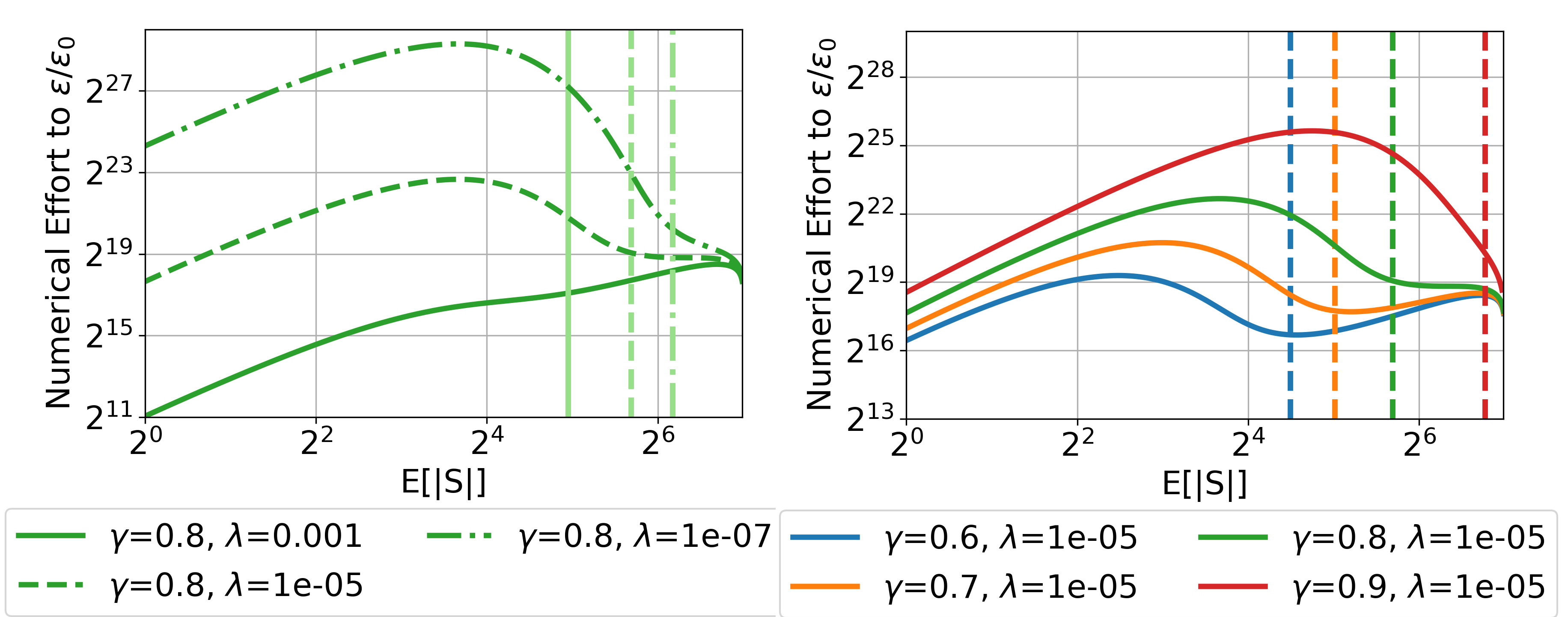
  (right) Numerical effort for polynomial decay.

Figure 1: In (a) we consider exponentially decreasing eigenvalues. In (b) (left) we plot the relationship between $p$ and $\mathbb{E}[\hat{S}]$ for exponential decay. In (b) (right) we show the numerical effort for polynomial decay.

5.2 Exponentially decreasing spectrum

Let $\{\lambda_{i}\}_{i=1}^{d}$ be the eigenvalues of $\mathbf{M}$ in decreasing order. Suppose that the eigenvalue decay is exponentially decreasing:

$$\lambda_{i}=C\gamma^{i}+C\lambda\text{ for }\gamma<1.$$

Motivation

A classical motivating example for the exponential eigenvalue decay is the squared exponential kernel, where an analytical form of the decay can be derived for normally distributed data (Rasmussen and Williams,, 2006). In particular, assuming $x\sim\mathcal{N}(0,\eta^{2})$, and using the kernel function $k(x,y)=\exp\big{(}-\frac{(x-y)^{2}}{2l^{2}}\big{)}$ in one dimension, the eigenvalues satisfy $\lambda_{k}\leq C\gamma^{k}$ for a general constant $C$ independent of $k$, where

$$\gamma=\frac{2\eta^{2}}{l^{2}+2\eta^{2}+\sqrt{l^{2}+2\eta^{2}}}.$$ (11)

Complexity

For the ease of exposition, suppose that $\gamma^{q+1}\leq\lambda\leq\gamma^{q}$, where $\lambda$ is the regularization constant and $q\in[d]$. Intuitively, this means that the regularization parameter flattens the decay at $\gamma^{q+1}$, which will play a role in the analysis.

To control the expected size $\mathbb{E}[|\hat{S}|]$ of determinantal sampling, let $\alpha(p)=C\gamma^{p}$, where $p\in[1,d]$. We get:

$$\mathbb{E}[|\hat{S}|]\stackrel{{\scriptstyle\eqref{eq:expected_size}}}{{\leq}}p+R_{d}(p,q)\quad\text{for}\quad\hat{S}\sim\operatorname{DPP}\big{(}\tfrac{1}{\alpha(p)}\mathbf{M}\big{)},$$

where $R_{d}(p,q)=\sum_{i=1}^{d-p}\frac{\gamma^{i}+\gamma^{q-p}}{\gamma^{i}+\gamma^{q-p}+1}$. Asymptotically, if $p\ll q$, i.e., the parameter $\alpha(p)$ dominates the regularization $C\lambda$, then the expected subset is $\mathbb{E}[|\hat{S}|]\approx p$. However, in the regime where $p=\Omega(q)$, the expected subset size rapidly goes up to $d$ (see Figure 1(b) (left)).

We now derive the convergence rate of RNM under determinantal sampling:

$$1-\sigma(\hat{S})\stackrel{{\scriptstyle\eqref{eq:corr}}}{{=}}\frac{C\gamma^{p}}{C\gamma^{d}+C\lambda+C\gamma^{p}}\geq\frac{1}{1+\gamma^{-p}(\gamma^{d}+\gamma^{q})}.$$

Likewise one can see that the convergence rate improves exponentially with $p$.

Numerical effort

From Theorem 5, we know that in order to reach an $\epsilon$ accurate solution from the initial accuracy $\epsilon_{0}=f(x^{0})-f(x^{*})$ under the convergence rate $\epsilon\leq(1-\sigma)^{T}\epsilon_{0}$, the number of needed steps can be bounded by

$$T\leq\frac{\log\left({\epsilon_{t}}\right)-\log\left({\epsilon_{0}}\right)}{\log(1-\sigma)}.$$ (12)

Using the bound derived for $1-\sigma(\hat{S})$, we obtain $T\leq\big{(}\log(\frac{1}{\epsilon_{t}})-\log(\frac{1}{\epsilon_{0}})\big{)}\big{(}\frac{\gamma^{p}}{\gamma^{d}+\gamma^{q}}+1\big{)}$. Since, the computation step is dominated by the inversion operation $\mathcal{O}(\mathbb{E}[|\hat{S}|]^{3})$, the number of arithmetic operations is

$$\mathcal{O}\left(\mathbb{E}[|S|]^{3}\cdot T\right)\leq\mathcal{O}\left(\big{(}p+R_{d}(p,q)\big{)}^{3}\frac{\gamma^{p}}{\gamma^{d}+\gamma^{q}}\right).$$

The upper bound on the numerical effort in the previous equation has two regimes. At first, for small subset sizes it is increasing, but then exponential decay starts to dominate and using larger blocks significantly improves the convergence rate. Finally it flattens around $\mathbb{E}[|\hat{S}|]=q$. Note that when $\lambda\approx\gamma^{q}$, i.e., for $q=\frac{\log(\lambda)}{\log(\gamma)}$, this phenomenon is visualized in Figure 1(a) where the vertical bars correspond to $q$. In the regime where $d\approx q$, inverting the whole matrix seems to be the best option. When $q<d$, the term $\gamma^{q}$ dominates the term $\gamma^{d}$, and the best subset size is either 1 or on the order of $q$, depending on the value of $\lambda$.

These observations are contrary to the intuition from the previous works. We suspect that, due to fixed memory fetching costs, for small sizes the initial phase is unobserved but the second phase should be observed. Figure 1(a) suggests that for sufficiently small values of $\lambda$ the numerical performance is maximized at the attenuation point $q$ and the predicted optimal block size is $\frac{\log(\lambda)}{\log(\gamma)}$.

5.3 Polynomially decaying spectrum

Suppose that the eigenvalues $\{\lambda_{i}\}_{i=1}^{d}$ are decreasing polynomially, i.e., so that $\lambda_{i}=Ci^{-s}+C\lambda$ for $s>1$.

Motivation

For example, consider a Matérn kernel of order $s$, which has the form $k(x,y)=C_{2}B_{s}(\left\lVert x-y\right\rVert)\exp(-C_{1}\left\lVert x-y\right\rVert)$, where $C_{1}$, $C_{2}$ are constants, and $B_{s}(d)$ is a modified Bessel function of order $s$ (see Rasmussen and Williams,, 2006). This class of kernels exhibits asymptotically polynomial decay of eigenvalues (see Seeger et al.,, 2008).

Complexity

Suppose, $\lambda=q^{-s}$ for $q\in[1,\infty)$. To control the expected size let us parameterize the tuning parameters as $\alpha=Cp^{-s}$, where $C$ is a suitable general constant. Then the convergence rate becomes:

$$1-\sigma(\hat{S})=\frac{p^{-s}}{d^{-s}+p^{-s}+q^{-s}}=\frac{1}{(p/d)^{s}+(p/q)^{s}+1}$$

and $\mathbb{E}[|\hat{S}|]=\sum_{i=1}^{d}\frac{i^{-s}+q^{-s}}{i^{-s}+p^{-s}+q^{-s}}$. If $p\ll q$, we can establish by integral approximation that $\mathbb{E}[|S|]\approx\mathcal{O}(p)$, otherwise the expected size grows faster. Additionally, with increasing $p$ the convergence rate always improves.

Numerical Effort

When $p\ll q$, similarly as in the preceding subsection, the numerical cost becomes $\mathcal{O}\big{(}p^{3}(\frac{d^{s}q^{s}}{p^{s}(q^{s}+d^{s})})\big{)}$. This suggests that for $s\geq 3$ the total numerical cost decreases for larger subsets, while for the problems with smaller $s$, the cost increases. In general, it is difficult to obtain general insights from the formulas, but the visalization in Figure 1b (right) suggests that if the regularization constant is large (small $q$), even problems with large $s$ might incur more cost as the subset size increases.

This suggests that small block sizes matching the memory fetching costs should be optimal if either the regularization is large or if $s$ is small. With the same assumption, if the desired accuracy is very high, performing full matrix inversion can be more efficient, corresponding to $\mathbb{E}[|\hat{S}|]\rightarrow d$ in Figure 1b (right). Note that increasing the accuracy to which we optimize the problem shifts the curves up in the logarithmic plot, while keeping the end point fixed.

(a) Sparse spectrum, rank of $\mathbf{K}$ shown.

(b) Exponential decay, varying lengthscale $\gamma$, for $\lambda=10^{-7}$

Figure 2: For Gaussian data, RNM exhibits similar behavior under DPP and uniform ($\tau$-nice) samplings.

5.4 Sparse spectrum

Suppose that only $s$ out of the $d$ eigenvalues are relatively large, while the remaining ones are very small. This scenario occurs with a linear kernel where the number of large eigenvalues corresponds to the number of features, and the remaining ones are proportional to the regularization parameter $\lambda$.

Complexity

For the ease of exposition, let the large eigenvalues all be equal to $\mu\gg\lambda$. Lemma 5 implies that if $\alpha=\sum_{i>k-1}^{d}\lambda_{i}$ then $\mathbb{E}[|\hat{S}|]\leq k$. The convergence rate can be split to two cases:

$$1-\sigma(\hat{S})=\begin{cases}\frac{d-k}{d-k+1}&\text{when }k\in[s,d-1],\\ 1-\frac{\lambda}{\mu}\frac{1}{d-k}+\mathcal{O}\left(\frac{\lambda^{2}}{\mu^{2}}\right)&\text{when }k\in[0,s).\end{cases}$$

We see that once $k\geq s$ a discontinuity in the spectrum implies a discontinuity in the convergence rate. Consequently, the optimal subset size is of the order of $s$ as long as $\frac{\lambda}{\mu}$ is sufficiently small.

6 EXPERIMENTS

We numerically validate the theoretical findings from the previous sections. Our main objective is to demonstrate that the convergence behavior of RNM under DPP sampling aligns well with the behavior of RNM under uniform sampling (called $\tau$-nice), which is more commonly used. This would suggest that our convergence analysis under DPP sampling is also predictive for other standard samplings. In addition to providing evidence for this claim, we also show that there are cases where DPP sampling leads to superior performance of RNM.

Even though there exist efficient algorithms for DPP sampling, we chose to use approximate ridge leverage score sampling as a cheaper proxy for DPP sampling, as suggested in a recent line of work (Dereziński,, 2019; Dereziński et al.,, 2019). The real data experiments were performed with sampling according to the $\frac{1}{2}$-approximate ridge leverage scores (Calandriello,, 2017). We always report the mean value of $10$ reruns of the experiment with the given parameters.

Gaussian Data

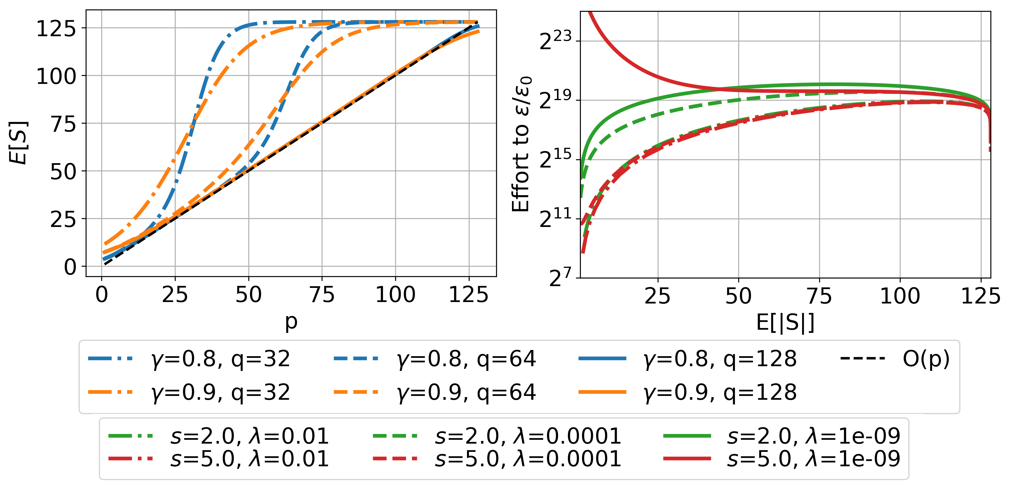
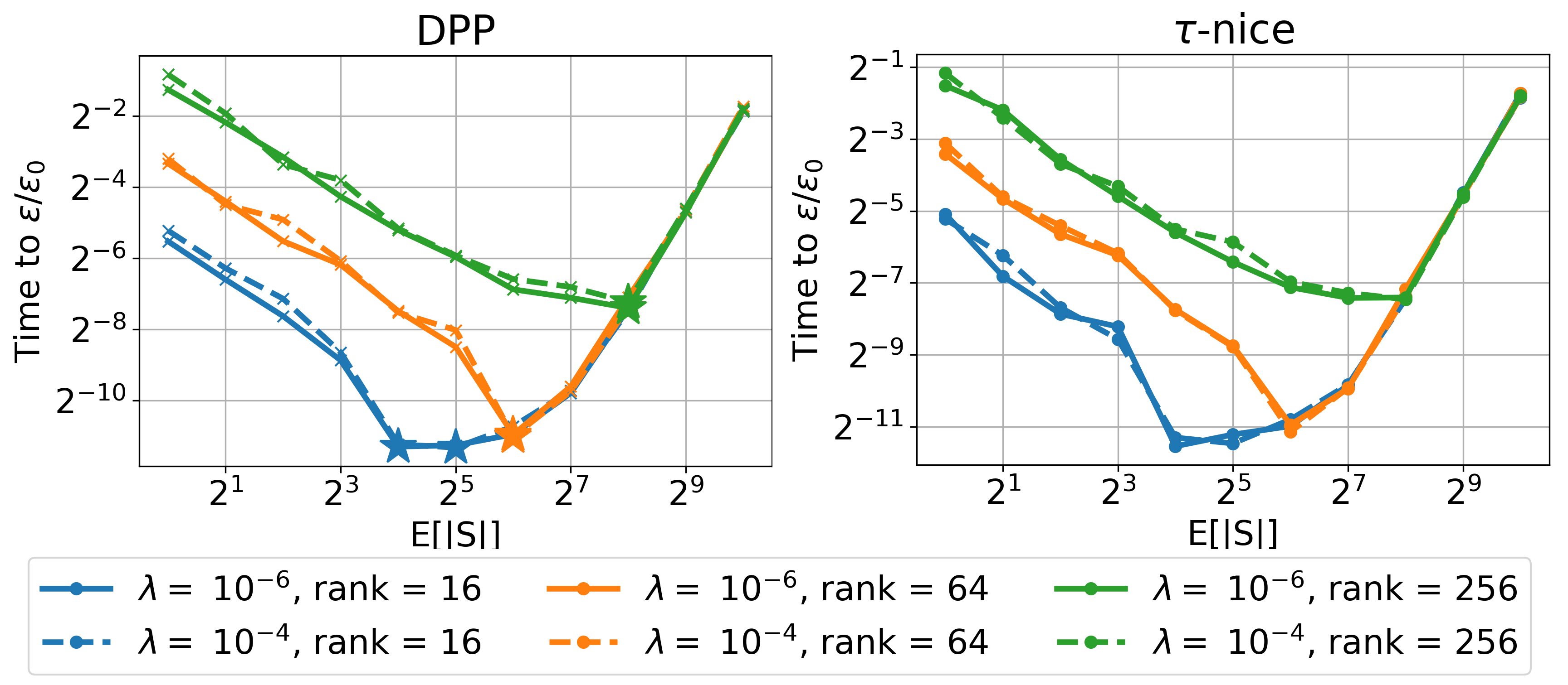
The first experiment deals with data sampled from a Gaussian distribution. The optimization using a kernel $\mathbf{K}$ with sparse spectrum (Figure 2(a)) verifies the theoretical findings that the optimal block size should be of the same order as $\operatorname{rank}(\mathbf{K})$. Using similarly generated data, and the relation in (11) to relate lengthscale $l$ and $\gamma$ of squared exponential kernel, we reproduce the prediction of the theory that for sharper decays the optimal expected size should be larger (see Figure 2(b), compared with theory, Figure 1(a)). The performance of DPP and uniform sampling is on par as the intuition suggests, since for normally distributed data even a uniform subsample provides good summary statistics.

Gaussian Mixture Data

Figure 3: Gaussian mixture data - sparse spectrum, rank of kernel $\mathbf{K}$ shown.

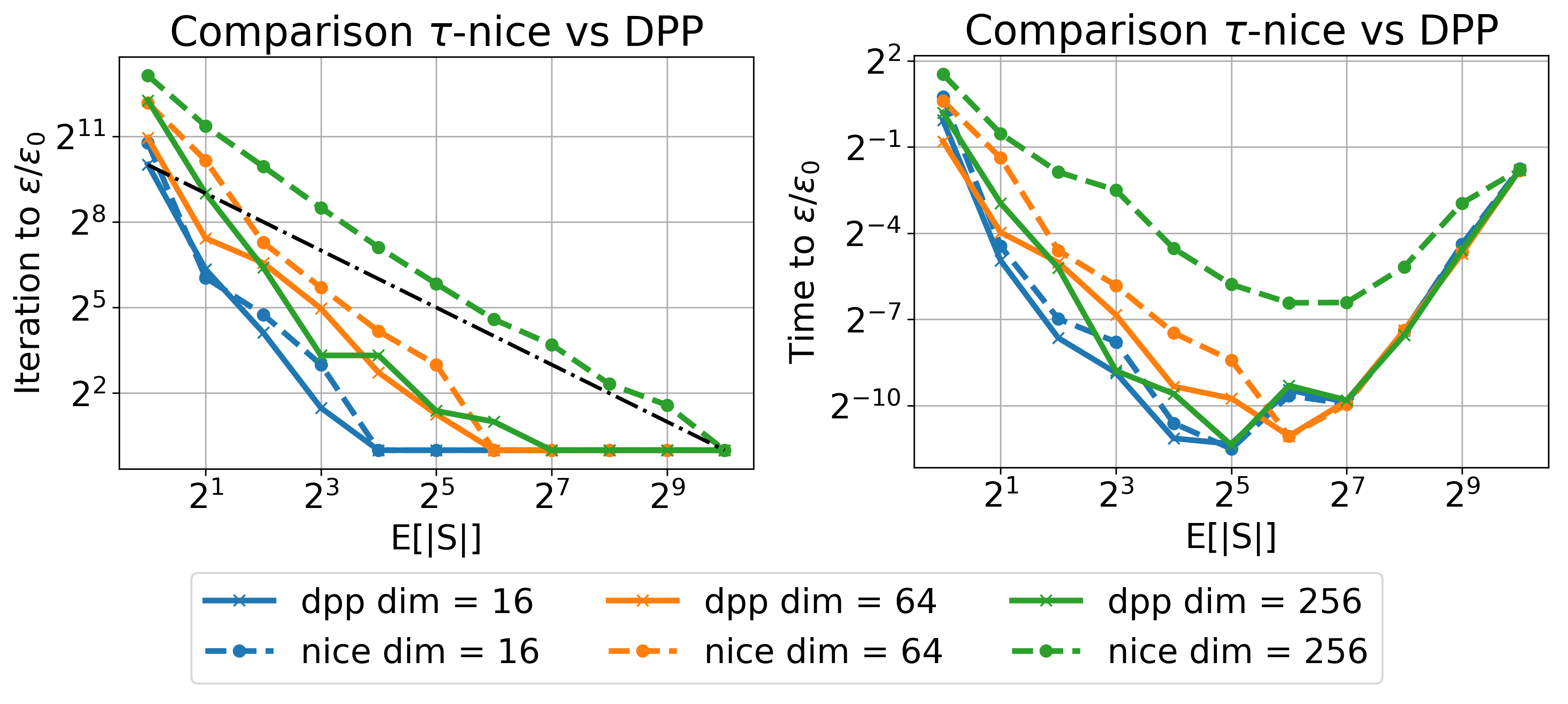
Akin to results from the sketching literature (e.g., see Dereziński and Warmuth,, 2018), we suspect that the superior convergence of DPP sampling over uniform presents itself primarily if the dataset is heterogeneous. By heterogeneity we mean that a uniform subsampling of the points is likely not a good summary of the dataset. Consider a dataset where the points are sampled from a Gaussian Mixture Model with $8$ clusters that are equally likely. In order to have a good summary, a point from each cluster should be present in the sample. DPP samples are generally more diverse than uniform samples which makes it more likely that they will cover all the clusters. In Figure 3, we see that DPP significantly outperforms uniform sampling for this dataset because it allows RNM to solve more representative subproblems.

Real Data Experiments

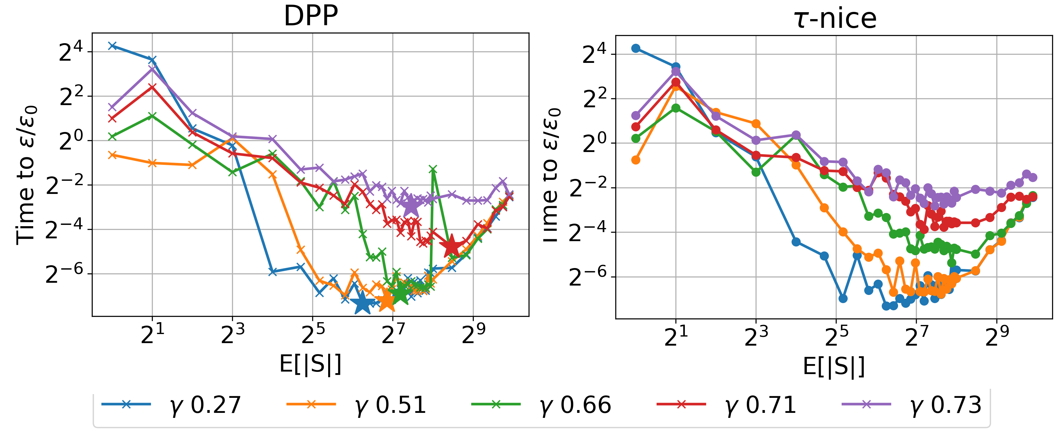
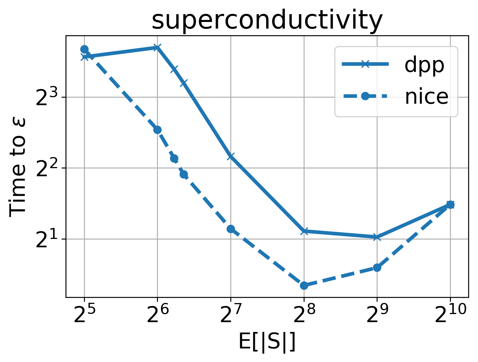
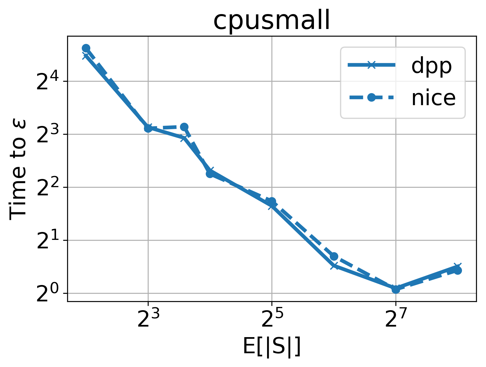
We perform two real data experiments on standard UCI datasets where we optimize until statistical precision. In Figure 4a, we optimize linear ridge regression on the superconductivity dataset. Next, in Figure 4b we fit kernel ridge regression with squared exponential kernel on the cpusmall dataset. For both datasets, the optimal subset size under DPP sampling roughly matches the optimal size under uniform sampling. Moreover, in the case of the superconductivity dataset, as suggested by the theory for linear kernels, the optimal size is of the same order as the feature dimensionality.

(a) $n=1460$ and $d=81$.

(b) $n=2191$ and $d=12$.

Figure 4: Experiments on real data.

7 CONCLUSION

We analyzed a sampling strategy for the Randomized Newton Method, where coordinate blocks of the Hessian over-approximation are sampled according to their determinant. This sampling allows for a simple interpretation of the convergence rate of the algorithm, which was previously not well understood. We demonstrated that for empirical risk minimization this convergence analysis allows us to predict the optimal size for the sampled coordinate blocks in order to minimize the total computational cost of the optimization.

Acknowledgments

This work was supported by SNSF grant 407540_167212 through the NRP 75 Big Data program. Also, MD thanks the NSF for funding via the NSF TRIPODS program.

Supplementary Material:

Convergence Analysis of Block Coordinate Algorithms

with Determinantal Sampling

Appendix A PROOFS

A.1 DPPs

Proof of Theorem 1.

First, assume that $\alpha=1$. Since $\mathbf{M}\succ\mathbf{0}$, we have $\det(\mathbf{M}_{SS})>0$ for all $S\subseteq[d]$. We will next use the following standard determinantal formula which holds for any $v\in\mathbb{R}^{d}$ and any invertible matrix $\mathbf{M}$:

$$\det(\mathbf{M})v^{\top}\mathbf{M}^{-1}v=\det(\mathbf{M}+vv^{\top})-\det(\mathbf{M}).$$ (13)

Applying this formula to the submatrices of $\mathbf{M}$ and denoting by $v_{S}$ the sub-vector of $v$ indexed by $S$, we show that for any $v\in\mathbb{R}^{d}$:

$$v^{\top} \mathbb{E}\big{[}(\mathbf{M}_{S})^{+}\big{]}v=\sum_{S\subseteq[d]}\frac{\det(\mathbf{M}_{SS})}{\det(\mathbf{I}+\mathbf{M})}v_{S}^{\top}\mathbf{M}_{SS}^{-1}v_{S}$$

$${\eqref{eq:pr0}}\ =\sum_{S\subseteq[d]}\frac{\det(\mathbf{M}_{SS}+v_{S}v_{S}^{\top})-\det(\mathbf{M}_{SS})}{\det(\mathbf{I}+\mathbf{M})}$$

$$=\frac{\sum_{S}\det([\mathbf{M}+vv^{\top}]_{SS})-\sum_{S}\det(\mathbf{M}_{SS})}{\det(\mathbf{I}+\mathbf{M})}$$

(Lemma 1) $$=\frac{\det(\mathbf{I}+\mathbf{M}+vv^{\top})-\det(\mathbf{I}+\mathbf{M})}{\det(\mathbf{I}+\mathbf{M})}$$

$${\eqref{eq:pr0}}\ =\frac{\det(\mathbf{I}+\mathbf{M})\,v^{\top}(\mathbf{I}+\mathbf{M})^{-1}v}{\det(\mathbf{I}+\mathbf{M})}$$

$$=v^{\top}(\mathbf{I}+\mathbf{M})^{-1}v.$$

Since the above holds for all $v$, the equality also holds for the pd. matrices. To obtain the result with $\alpha\neq 1$, it suffices to replace $\mathbf{M}$ with $\frac{1}{\alpha}\mathbf{M}$. ∎

Proof of Lemma 3.

The eigenvalues of $\mathbf{M}(\alpha\mathbf{I}+\mathbf{M})^{-1}$ are $\frac{\lambda_{i}}{\lambda_{i}+\alpha}$ so

$$\mathbb{E}[|S|] =\sum_{i=1}^{d}\frac{\lambda_{i}}{\lambda_{i}+\alpha}=\sum_{i=1}^{d}\frac{\lambda_{i}}{\lambda_{i}+\sum_{j\geq k}\lambda_{j}}$$

$$=\sum_{i<k}^{d}\frac{\lambda_{i}}{\lambda_{i}+\sum_{j\geq k}\lambda_{j}}+\sum_{i\geq k}^{d}\frac{\lambda_{i}}{\lambda_{i}+\sum_{j\geq k}\lambda_{j}}$$

$$<(k-1)+1=k,$$

which concludes the proof. ∎

A.2 Convergence Analysis

Proof of Theorem 2.

$$\sigma_{1} \stackrel{{\scriptstyle\eqref{eq:sigma_1}}}{{=}} \lambda_{\min}\left(\mathbf{M}^{1/2}\left({\alpha}\mathbf{I}+\mathbf{M}\right)^{-1}\mathbf{M}^{1/2}\right)$$ (14)

$$= \lambda_{min}\left(\left({\alpha}\mathbf{M}^{-1}+\mathbf{I}\right)^{-1}\right)$$ (15)

$$= \frac{1}{\lambda_{\max}\left({\alpha}\mathbf{M}^{-1}+\mathbf{I}\right)}=\frac{1}{1+{\alpha}\lambda_{\max}(\mathbf{M}^{-1})}$$ (16)

$$= \frac{\mu}{\mu+\alpha}$$ (17)

where $\mu=\lambda_{\min}(\mathbf{M})$. ∎

Proof of Proposition 1.

By definition,

$$\frac{1}{\sigma(k+1)}=1+\frac{\sum_{i>k}^{d}\lambda_{i}}{\lambda_{d}}=1+\frac{\sum_{i>{k-1}}^{d}\lambda_{i}-\lambda_{k}}{\lambda_{d}}=\frac{1}{\sigma(k)}-\frac{\lambda_{k}}{\lambda_{d}}$$

Rearranging,

$$\frac{1}{\sigma(k)}=\frac{1}{\sigma(k+1)}+\frac{\lambda_{k}}{\lambda_{d}}\implies\sigma(k)=\frac{\sigma(k+1)\lambda_{d}}{\lambda_{d}+\lambda_{k}\sigma(k+1)}$$

Dividing the denominator and the numerator by $\lambda_{d}$ finishes the proof.

∎

A.3 Dual convergence rate

The dual convergence rate established in Qu et al., (2016) relies on the notion of expected separable over-approximation. Namely, the existence of $v\in\mathbb{R}^{d}$ s.t. $\mathbb{E}[\mathbf{M}_{S}]\preceq\mathbf{D}(p\circ v)$, where $p$ is the vector of marginal probabilities. In case of DPP sampling, one can choose $v=\operatorname{diag}(\mathbf{M})\circ\operatorname{diag}(\mathbf{M}(\mathbf{M}+\alpha\mathbf{I})^{-1})^{-1}$, and apply dual convergence results established in this literature. By $\circ$ we denote element-wise product.

Appendix B LEVERAGE SCORE SAMPLING VS DPP SAMPLING

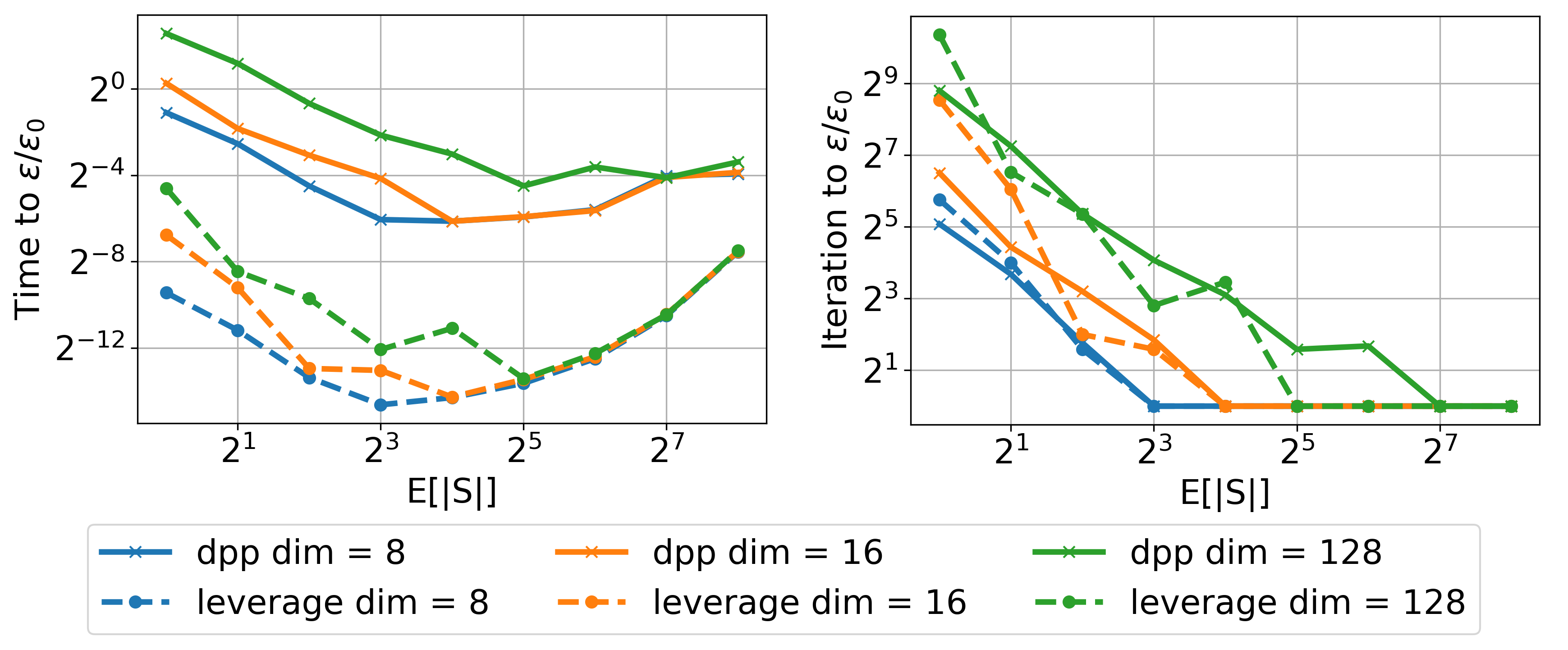
We perform a simple experiment on the Gaussian Mixtures dataset where the matrix has a sparse spectrum. In Figure 5 we see that the optimization process is influenced minimally.

Figure 5: Comparison of leverage score sampling and DPP

Appendix C RELATIVE SMOOTHNESS AND RELATIVE STRONG CONVEXITY

Recent works such as (Gower et al.,, 2019) and (Karimireddy et al.,, 2018) introduce the concepts of relative-smoothness, relative strong convexity and $c$-stability. These are weaker conditions than assumed in this paper. With these conditions, the proof techniques used to analyze coordinate descent algorithms are applicable to Newton-like algorithms, where instead of a fixed matrix $\mathbf{M}$, the actual Hessian $\mathbf{H}(x)$ can be used. The extension to $c-$stability is done trivially in Theorem 2 of Karimireddy et al., (2018), here we focus on a slightly more elaborate connection with relative smoothness and relative strong-convexity.

Assumption 3 (Gower et al., (2019)).

There exists a constant $\tilde{L}\geq\tilde{\mu}$ such that for all $x,y\in\mathcal{Q}\subseteq\mathbb{R}^{d}$, where $\mathcal{Q}:=\{x\in\mathbb{R}^{d}:f(x)\leq f(x_{0})\}$:

$$f(x)\leq f(y)+\braket{\nabla f(y),x}+\frac{\tilde{L}}{2}\left\lVert x-y\right\rVert_{\mathbf{H}(y)}$$ (19)

and

$$f(x)\geq f(y)+\braket{\nabla f(y),x}+\frac{\tilde{\mu}}{2}\left\lVert x-y\right\rVert_{\mathbf{H}(y)}.$$ (20)

Now the task is to analyze the algorithm with the following update rule, which is identical to general Newton rule when $S=[d]$,

$$x_{k+1}=x_{k}-\gamma(\mathbf{H}(x_{k})_{S_{k}})^{+}\nabla f(x_{k}).$$ (21)

We fix a particular choice of $\gamma=1/\tilde{L}$. This should be contrasted with the update rule $\eqref{eq:update}$.

Now given these assumption, we are able to show that the constant akin to $\sigma(\hat{S})$ appears in the analysis of this algorithm by utilizing the notions from (Gower et al.,, 2019). We sacrifice generality for the sake of brevity, and assume that range of $\mathbf{H}(x)$ spans whole $\mathbb{R}^{d}$ for each $x\in\mathcal{Q}$. Then, the following quantities resembling $\sigma(\hat{S})$ appear in the convergence analysis of the update rule (21)

$$\hat{\sigma}(\hat{S},x)=\lambda_{\min}\left(\mathbb{E}_{\hat{S}}\left[\mathbf{H}^{1/2}(x)(\mathbf{H}(x)_{\hat{S}})^{+}\mathbf{H}(x)^{1/2}\right]\right)$$ (22)

and

$$\hat{\sigma}(\hat{S})=\min_{x\in\mathcal{Q}}\hat{\sigma}(\hat{S},x)$$

Theorem 3 (Theorem 3.1 of Gower et al., (2019), modified).

Let $f$ satisfy Assumption 3, and let $\mathbf{H}(x)$ be the Hessian at $x$ having range that spans whole $\mathbb{R}^{d}$ for all $x$. Then

$$\mathbb{E}_{\hat{S}}[f(x_{k+1})-f(x^{*})]\leq\left(1-\frac{\hat{\sigma}(\hat{S},x_{k})\mu}{L}\right)(f(x_{k})-f(x^{*}),$$

and

$$\mathbb{E}_{\hat{S}}[f(x_{k})-f(x^{*})]\leq\left(1-\frac{\hat{\sigma}(\hat{S})\mu}{L}\right)^{k}(f(x_{0})-f(x^{*}),$$

where $\hat{\sigma}(\hat{S})=\min_{x\in\mathcal{Q}}\hat{\sigma}(\hat{S},x)$ as in Equation (22).

Proof.

Minimizing the upper bound in (19) restricted to coordinates in $S_{k}$, we arrive at,

$$f(x_{k+1})-f(x_{k}) \stackrel{{\scriptstyle\eqref{eq:smooth}}}{{\leq}} -\frac{1}{2\tilde{L}}\braket{\nabla f(x_{k}),(\mathbf{H}(x_{k})_{S_{k}})^{+}\nabla f(x_{k})}$$

$$\mathbb{E}[f(x_{k+1})-f(x_{k})] \leq -\frac{1}{2\tilde{L}}\braket{\nabla f(x_{k}),\mathbb{E}_{\hat{S}}[(\mathbf{H}(x_{k})_{S_{k}})^{+}]\nabla f(x_{k})}$$

$$\stackrel{{\scriptstyle\eqref{eq:rconvex},\eqref{eq:sigmahat}}}{{\leq}} -\frac{\mu}{L}\hat{\sigma}(\hat{S},x)(f(x_{k})-f(x^{*}))$$

$$\leq -\frac{\mu}{L}\hat{\sigma}(\hat{S})(f(x_{k})-f(x^{*}))$$

rearranging finishes the proof. ∎

The following corollary states that with DPP sampling, the update rule in (21) can have a more interpretable convergence rate than stated in the Theorem 3.

Corollary 1 (of Theorem 3).

Under the assumption of Theorem 3, let additionally $S_{k}$ be a sample from sampling $\hat{S}_{k}\sim\operatorname{DPP}(\frac{1}{\alpha}\mathbf{H}(x_{k}))$, then

$$\mathbb{E}_{\hat{S}_{k}}[f(x_{k+1})-f(x^{*})]\leq\left(1-\left(\frac{\lambda(x_{k})}{\lambda(x_{k})+\alpha}\right)\frac{\mu}{L}\right)(f(x_{k})-f(x^{*}),$$

where $\lambda(x_{k})=\lambda_{\min}(\mathbf{H}(x_{k}))$.

The following lemma relates the complexity quantity defined above to the definition of $\sigma(\hat{S})$ used in the main body of this paper. Note that $\hat{\sigma}$ is larger than $\sigma$, even if the fixed over-approximation exists, as previously we assumed the over-approximation to be valid globally not just in $\mathcal{Q}$.

Lemma 7.

If for all $x\in\mathcal{Q}$, $\mathbf{M}\succeq\mathbf{H}(x)\succeq\kappa\mathbf{M}\succ 0$, then

$$\hat{\sigma}(\hat{S})\geq\kappa\sigma(\hat{S}).$$

The relative smoothness, and strong-convexity can be chosen to be $\tilde{L}=1$, and $\tilde{\mu}=1$, respectively.

Proof.

$$\hat{\sigma}(\hat{S}) = \min_{x\in\mathcal{Q}}\min_{v\in\mathbb{R}^{d}}\frac{\braket{v,\mathbb{E}_{\hat{S}}\left[\mathbf{H}^{1/2}(x)(\mathbf{H}(x)_{\hat{S}})^{+}\mathbf{H}(x)^{1/2}\right]v}}{{\left\lVert v\right\rVert_{2}^{2}}}=\min_{v\in\mathbb{R}^{d}}\min_{x\in\mathcal{Q}}\frac{\braket{v,\mathbb{E}_{\hat{S}}\left[\mathbf{H}^{1/2}(x)(\mathbf{H}(x)_{\hat{S}})^{+}\mathbf{H}(x)^{1/2}\right]v}}{\left\lVert v\right\rVert_{2}^{2}}$$

$$\geq \min_{v\in\mathbb{R}^{d}}\frac{\braket{v,\mathbb{E}_{\hat{S}}\kappa\left[\mathbf{M}^{1/2}(\mathbf{M}_{\hat{S}})^{+}\mathbf{M}^{1/2}\right]v}}{\left\lVert v\right\rVert_{2}^{2}}=\kappa\sigma(\hat{S})$$

∎

Appendix D OTHER SAMPLINGS

The convergence properties of RNM with determinantal sampling depend solely on the spectral properties of $\mathbf{M}$. This is not true of other common samplings such as $\tau$-nice. Indeed we can improve or worsen the performance of $\tau$-nice sampling when $\mathbf{M}$ is transformed via spectrum preserving operation such as unitary transformation

$$\mathbf{M}\leftarrow\mathbf{R}^{\top}\mathbf{M}\mathbf{R},\text{ where }\mathbf{R}^{\top}\mathbf{R}=\mathbf{I}.$$

Suppose that we are given an eigenvalues of the matrix $\mathbf{M}$, for any sampling $\hat{S}$ is it possible to find a spectrum preserving rotation such that $\sigma(\hat{S})$ is at least as small as $\sigma(\hat{S}_{\operatorname{DPP}})$ which corresponds to DPP sampling with the same expected cardinality? The answer turns out to be negative, and we show counter-example.

Remark 2 (Counter-example).

Let $\hat{S}_{1}$ be a sampling such that $[n]$ is sampled with $1/2$ probability and $\emptyset$ and $1/2$ probability. The expected size of the subset $\mathbb{E}[|\hat{S}_{1}|]=d/2$ and $\sigma(\hat{S}_{1})=\frac{1}{2}$ irrespective of the matrix $\mathbf{M}$.

Suppose matrix $\mathbf{M}$ has degenerate spectrum such that $\lambda$ is eigenvalue with multiplicity $d/2$ and $\mu$ is eigenvalue with $d/2$ multiplicity where $\lambda<\mu$. In order s.t. $\mathbb{E}[|S_{\operatorname{DPP}}|]=\frac{d}{2}$, $\alpha=\sqrt{\lambda\mu}$, then $\sigma(\hat{S}_{\operatorname{DPP}})<\frac{1}{2}$.

In what circumstances does DPP sampling perform better than a uniform sampling? First, we consider circumstances where uniform sampling is optimal.

D.1 Uniform sampling

It is important to allow for variation in the off-diagonal of $\mathbf{M}$. If we consider only diagonal $\mathbf{M}$, the optimal sampling is uniform sampling.

Lemma 8.

Let $\mathbf{M}$ be diagonal. The quantity $\sigma(\hat{S})$ of a sampling over a power set $P([d])$ constrained by $\mathbb{E}[|\hat{S}|]=k$ is maximized for uniform samplings.

Proof of Lemma 8 .

We want to maximize the minimum eigenvalue of a matrix $\mathbf{M}^{1/2}\mathbb{E}[(\mathbf{M}_{S})^{-1}]\mathbf{M}^{1/2}$. For a diagonal $\mathbf{M}$ we know that $(\mathbf{M}_{S})^{-1}=(\mathbf{M}^{-1})_{S}$. Hence, $\mathbf{M}^{1/2}\mathbb{E}[(\mathbf{M}_{S})^{-1}]\mathbf{M}^{1/2}\mathbf{D}(p)$, where $p$ is a vector of marginals $p_{i}=P(i\in\hat{S})$. Hence, the minimum eigenvalue is the minimum marginal probability subject to a constraint that $\mathbb{E}[|S|]=\sum_{j=1}^{d}P(j\in\hat{S})\leq k$. This leads to an optimum where $P(i\in\hat{S})=P(j\in\hat{S})$ for all $i,j\in[d]$. Hence the optimal sampling distribution is uniform. ∎

D.2 Parallel Sampling

The parallel extension of the update method 3 has been considered in Mutný and Richtárik, (2018) and Karimireddy et al., (2018). Namely, the authors consider a case, when the updates with $c$ machines are aggregated together to form a single update in the form $\approx\frac{1}{b}\sum_{j=1}^{c}(\mathbf{M}_{S_{j}})^{+}$, where $b$ is the aggregating parameter. It is known that for parallel disjoint samplings the convergence rate increases linearly with the number of processors. For independent samplings the aggregating parameter $b$ depends on the quantity,

$$\theta(\hat{S})=\lambda_{\max}(\mathbf{M}^{1/2}\mathbb{E}[(\mathbf{M}_{\hat{S}})^{+}]\mathbf{M}^{1/2})$$

which in the case of DPP sampling is equal to $\theta=\frac{\lambda_{1}}{\lambda_{1}+\alpha}$. The quantity $\theta(\hat{S})\in[\sigma(\hat{S}),1]$, and as $\theta\rightarrow 1$, the aggregation operation becomes averaging $b\rightarrow c$. For DPP sampling, we can see an inverse relationship between increasing $\sigma(\hat{S})$ by increasing block size, which inherently makes the parallelization problem more difficult by increasing $\theta(\hat{S})$.

References

- Alaoui and Mahoney, (2015) Alaoui, A. E. and Mahoney, M. W. (2015). Fast randomized kernel ridge regression with statistical guarantees. In Proceedings of the 28th International Conference on Neural Information Processing Systems, pages 775–783, Montreal, Canada.
- Allen-Zhu et al., (2016) Allen-Zhu, Z., Qu, Z., Richtárik, P., and Yuan, Y. (2016). Even faster accelerated coordinate descent using non-uniform sampling. In International Conference on Machine Learning, pages 1110–1119.
- Anari et al., (2016) Anari, N., Gharan, S. O., and Rezaei, A. (2016). Monte carlo markov chain algorithms for sampling strongly rayleigh distributions and determinantal point processes. In Feldman, V., Rakhlin, A., and Shamir, O., editors, 29th Annual Conference on Learning Theory, volume 49 of Proceedings of Machine Learning Research, pages 103–115, Columbia University, New York, New York, USA. PMLR.
- Blanchard et al., (2007) Blanchard, G., Bousquet, O., and Zwald, L. (2007). Statistical properties of kernel principal component analysis. Machine Learning, 66(2):259–294.
- Borsos et al., (2019) Borsos, Z., Curi, S., Levy, K. Y., and Krause, A. (2019). Online variance reduction with mixtures. In Proc. International Conference on Machine Learning (ICML).
- Borwein and Zhu, (2005) Borwein, J. and Zhu, Q. (2005). Techniques of Variational Analysis. Springer-Verlag New York.
- Calandriello, (2017) Calandriello, D. (2017). Efficient Sequential Learning in Structured and Constrained Environments. PhD thesis, Inria Lille Nord Europe-Laboratoire CRIStAL-Université de Lille.
- Dereziński, (2019) Dereziński, M. (2019). Fast determinantal point processes via distortion-free intermediate sampling. In Proceedings of the 32nd Conference on Learning Theory.
- Dereziński et al., (2019) Dereziński, M., Calandriello, D., and Valko, M. (2019). Exact sampling of determinantal point processes with sublinear time preprocessing. CoRR, abs/1905.13476.
- Dereziński and Warmuth, (2018) Dereziński, M. and Warmuth, M. K. (2018). Reverse iterative volume sampling for linear regression. Journal of Machine Learning Research, 19(23):1–39.
- Dünner et al., (2016) Dünner, C., Forte, S., Takáč, M., and Jaggi, M. (2016). Primal-dual rates and certificates. In Proceedings of The 33rd International Conference on Machine Learning, pages 783–792.
- Gower et al., (2019) Gower, R., Koralev, D., Lieder, F., and Richtarik, P. (2019). RSN: Randomized subspace Newton. In Wallach, H., Larochelle, H., Beygelzimer, A., d Alché-Buc, F., Fox, E., and Garnett, R., editors, Advances in Neural Information Processing Systems 32, pages 614–623. Curran Associates, Inc.
- Gower and Richtárik, (2015) Gower, R. M. and Richtárik, P. (2015). Randomized iterative methods for linear systems. SIAM. J. Matrix Anal. & Appl., 36(4), 1660–1690, 2015.
- Hanzely and Richtárik, (2018) Hanzely, F. and Richtárik, P. (2018). Accelerated coordinate descent with arbitrary sampling and best rates for minibatches. arXiv preprint arXiv:1809.09354.
- Hough et al., (2006) Hough, J. B., Krishnapur, M., Peres, Y., Virág, B., et al. (2006). Determinantal processes and independence. Probability surveys, 3:206–229.
- Johnson and Zhang, (2013) Johnson, R. and Zhang, T. (2013). Accelerating stochastic gradient descent using predictive variance reduction. In Proceedings of the 26th International Conference on Neural Information Processing Systems - Volume 1, NIPS’13, pages 315–323, USA. Curran Associates Inc.
- Karimireddy et al., (2018) Karimireddy, S. P. R., Stich, S., and Jaggi, M. (2018). Adaptive balancing of gradient and update computation times using global geometry and approximate subproblems. In Storkey, A. and Perez-Cruz, F., editors, Proceedings of the Twenty-First International Conference on Artificial Intelligence and Statistics, volume 84 of Proceedings of Machine Learning Research, pages 1204–1213, Playa Blanca, Lanzarote, Canary Islands. PMLR.
- Kulesza and Taskar, (2012) Kulesza, A. and Taskar, B. (2012). Determinantal Point Processes for Machine Learning. Now Publishers Inc., Hanover, MA, USA.
- Ma et al., (2015) Ma, C., Virginia, S., Jaggi, M., Jordan, M. I., Richtárik, P., and Takáč, M. (2015). Adding vs. averaging in distributed primal-dual optimization. ICML.
- Macchi, (1975) Macchi, O. (1975). The coincidence approach to stochastic point processes. Advances in Applied Probability, 7(1):83–122.
- Mutný and Richtárik, (2018) Mutný, M. and Richtárik, P. (2018). Parallel stochastic newton method. Journal of Computational Mathematics, 36(3):405–426.
- Nguyen et al., (2017) Nguyen, L. M., Liu, J., Scheinberg, K., and Takáč, M. (2017). Sarah: A novel method for machine learning problems using stochastic recursive gradient. In Proceedings of the 34th International Conference on Machine Learning-Volume 70, pages 2613–2621. JMLR. org.
- Pilanci and Wainwright, (2015) Pilanci, M. and Wainwright, M. J. (2015). Newton sketch: A linear-time optimization algorithm with linear-quadratic convergence. arXiv preprint arXiv:1505.02250.
- Qu et al., (2016) Qu, Z., Richtárik, P., Takáč, M., and Fercoq, O. (2016). SDNA: Stochastic Dual Newton Ascent for Empirical Risk Minimization. Proceedings of The 33rd International Conference on Machine Learning.
- Qu and Richtárik, (2016) Qu, Z. and Richtárik, P. (2016). Coordinate descent with arbitrary sampling ii: Expected separable overapproximation. Optimization Methods and Software, 31(5):858–884.
- Rasmussen and Williams, (2006) Rasmussen, C. and Williams, C. (2006). Gaussian processes for machine learning. The MIT Press, Cambridge, doi, 10:S0129065704001899.
- Richtárik and Takác, (2013) Richtárik, P. and Takác, M. (2013). Distributed coordinate descent method for learning with big data.
- Richtárik and Takáč, (2015) Richtárik, P. and Takáč, M. (2015). On optimal probabilities in stochastic coordinate descent methods. Optimization Letters, pages 1–11.
- Richtárik and Takáč, (2016) Richtárik, P. and Takáč, M. (2016). Parallel coordinate descent methods for big data optimization. Mathematical Programming, 156(1):433–484.
- Rodomanov and Kropotov, (2019) Rodomanov, A. and Kropotov, D. (2019). A randomized coordinate descent method with volume sampling. arXiv preprint arXiv:1904.04587.
- Roosta-Khorasani and Mahoney, (2016) Roosta-Khorasani, F. and Mahoney, M. W. (2016). Sub-Sampled Newton Methods I: Globally Convergent Algorithms. ArXiv e-prints.
- Roosta-Khorasani and Mahoney, (2016) Roosta-Khorasani, F. and Mahoney, M. W. (2016). Sub-sampled newton methods ii: Local convergence rates. arXiv preprint arXiv:1601.04738.
- Seeger et al., (2008) Seeger, M. W., Kakade, S. M., and Foster, D. P. (2008). Information consistency of nonparametric gaussian process methods. IEEE Transactions on Information Theory, 54(5):2376–2382.
- Shalev-Shwartz and Ben-David, (2014) Shalev-Shwartz, S. and Ben-David, S. (2014). Understanding machine learning: From theory to algorithms. Cambridge university press.
- Shalev-Shwartz and Zhang, (2013) Shalev-Shwartz, S. and Zhang, T. (2013). Stochastic dual coordinate ascent methods for regularized loss. The Journal of Machine Learning Research, 14(1):567–599.
- Zhang et al., (2017) Zhang, C., Kjellström, H., and Mandt, S. (2017). Determinantal point processes for mini-batch diversification. In 33rd Conference on Uncertainty in Artificial Intelligence, UAI 2017, Sydney, Australia, 11 August 2017 through 15 August 2017. AUAI Press Corvallis.