Quantile Regression Modelling via Location and Scale Mixtures of Normal Distributions

Abstract

We show that the estimating equations for quantile regression can be solved using a simple EM algorithm in which the M-step is computed via weighted least squares, with weights computed at the E-step as the expectation of independent generalized inverse-Gaussian variables. We compute the variance-covariance matrix for the quantile regression coefficients using a kernel density estimator that results in more stable standard errors than those produced by existing software. A natural modification of the EM algorithm that involves fitting a linear mixed model at the M-step extends the methodology to mixed effects quantile regression models. In this case, the fitting method can be justified as a generalized alternating minimization algorithm. Obtaining quantile regression estimates via the weighted least squares method enables model diagnostic techniques similar to the ones used in the linear regression setting. The computational approach is compared with existing software using simulated data, and the methodology is illustrated with several case studies.

Keywords: Expectation Maximization (EM) algorithm, Generalized Alternating Minimization (GAM) algorithm, Mixed effects regression, model diagnostics.

1 Introduction

Quantile regression (QR) is used to predict how a certain percentile of a quantitative response variable, $Y$, changes with some predictors, $\mathbf{x}=(x_{1},\ldots,x_{p})$ and as a consequence offers an approach for examining how covariates influence the location, scale, and shape of the response distribution. It is assumed that the predictors $x_{j}$ and the $q$-th quantile of $Y$ are linearly related, and that $y_{1},\ldots,y_{n}$ are independent distributed as $P(y_{i}<y)=F(y-\mathbf{x}_{i}^{T}\bm{\beta}_{q})$, where $\bm{\beta}_{q}$ is a vector of unknown coefficients which depends on $q\in(0,1)$. (Henceforth, as usual, $\mathbf{x}_{i}^{T}\bm{\beta}_{q}$ will include the intercept, $\beta_{0,q}$.)

The idea of estimating a median regression slope based on minimizing sum of the absolute deviances has a long history that dates back to Boskovic, Edgeworth, and Laplace. A very special case of QR is when $q=0.5$ and the random errors $y_{i}-\mathbf{x}_{i}^{T}\bm{\beta}$ are assumed to be (i) normally distributed, (ii) with mean 0 and variance $\sigma^{2}$, and (iii) uncorrelated with the predictors. In this case, the relationship between $\mathbf{x}$ and the median of $Y$ is the same as between $\mathbf{x}$ and the mean of $Y$, and linear regression (LR) is used to estimate the rate of change in $Y$ for a unit change in each $x_{j}$, via the ordinary least squares (OLS) method. Yet, although QR is more versatile in the sense that it can be used to make more general predictions than just for the mean of $Y$, and although LR relies on more restrictive and sometimes unrealistic assumptions, and is sensitive to outliers, there is no doubt that for over a century LR has been vastly more popular in applications than QR. This is, perhaps, due to the fact that LR offers closed-form formulas for the model parameters, and also because, when the assumptions regarding the random error are valid, the distributional properties of the model parameters are known and can be used to perform inferential procedures. Inference in the QR setting is based on rank-based methods which are less powerful than their parametric counterparts in LR, or on computationally challenging resampling methods, such as the bootstrap. Another historical reason for favoring the linear regression framework is that it extends rather naturally to include complex error structures such as random effects.

In the LR framework, the normal model for the errors yields a convenient likelihood function which can be easily maximized with respect to $\bm{\beta}$. In practice, this is achieved through solving the estimating equation which is obtained by minimizing the negative of the log-likelihood, that is, by solving

$$\hat{\bm{\beta}}=\underset{\bm{\beta}}{\arg\min}\sum_{i=1}^{n}(y_{i}-\mathbf{x}_{i}^{T}\bm{\beta})^{2}\,.$$

So, numerically, the solution is obtained by minimizing the quadratic loss function, rather than directly maximizing the likelihood. Similarly, in the QR framework, the estimation of the regression parameters (for a specific quantile of interest, $q$) is done (e.g., Koenker and Hallock (2001); Koenker and Bassett (1978)) by solving an estimating equation involving the ‘check’ loss function (see Figure 1):

$$\hat{\bm{\beta}}_{q}=\underset{\bm{\beta}}{\arg\min}\sum_{i=1}^{n}\rho_{q}\left(y_{i}-\mathbf{x}_{i}^{T}\bm{\beta}\right)$$ (1)

where

$$\rho_{q}(u)=u\cdot(q-1_{[u<0]})\,,$$ (2)

and $1_{[u<0]}$ is the indicator function which equals 1 when the argument, $u$, is negative. Equation (1) does not lead to a closed-form formula for $\bm{\beta}_{q}$, but a numerical solution via algorithmic methods is feasible. For a comprehensive review of QR in general, see Koenker et al. (2005). For a different approach for estimating $\bm{\beta}_{q}$ using the majorization-minimization (MM) algorithm, see Hunter and Lange (2000).

Figure 1: The ‘check’ loss function ($q=0.2$)

The optimization problem (1) is equivalent to maximum likelihood estimation under the assumption that the errors in the linear model, $y_{i}=\mathbf{x}_{i}^{T}\bm{\beta}_{q}+u_{i}$, are an iid sample from an asymmetric Laplace distribution (ALD), with density given by

$$f(u|\alpha,q)=q(1-q)\exp\left\{-\rho_{q}(u/\alpha)\right\}/\alpha$$

Yu and Moyeed (2001). Methods for fitting quantile regression models for linear mixed models using the asymmetric Laplace distribution have been proposed; see, for example, Geraci and Bottai (2007), Geraci and Bottai (2014), and Galarza et al. (2017) who use an EM-type algorithm combined with numerical quadrature for fitting the QR model. Although it is possible to represent QR in terms of a likelihood function, the estimation procedure still requires numerical estimation of $\bm{\beta}_{q}$ and the inferential procedures are computationally inefficient because the loss function is not differentiable at 0. In a Bayesian approach to quantile regression, Kozumi and Kobayashi (2011) posited the ALD as the working likelihood to perform the inference and Yu and Moyeed (2001) proposed an efficient Gibbs sampling algorithm by using a location and scale mixture representation of the ALD.

We propose a new computational method for QR, using an implicit location and scale mixture model approach as in Kozubowski and Podgorski (2000). The computations needed to minimize (1) are typically formulated as a linear programming problem (Koenker and D’Orey (1987); Portnoy and Koenker (1997)) which allows for efficient computation. The utility of the location and scale mixture model representation used in this paper is that, conditional on a particular set of random variables, flexible approaches of a normal distribution modeling framework are at our disposal. The representation sets the stage for developing more complex QR models (see Section 6).

The underlying estimating equation we use is also (1), so the QR estimator obtained from our method is identical to the one obtained via traditional estimation, and therefore, it is consistent. However, our approach has a few advantages over the traditional method. First, it allows us to obtain a closed-form analytic solution to the regression problem. In fact, the solution is the well-known weighted least squares (WLS) estimator. Second, since our QR estimator is obtained via the weighted least squares method, it is possible to construct model diagnostic techniques akin to the ones used in the LR setting. Third, our method yields less variable estimates for the standard errors of the regression coefficients. Fourth, because the residuals are shown to be (conditionally) normally distributed, our method is easily extended to quantile regression in mixed models. Finally, parameter estimation is done efficiently via an Expectation Maximization (EM) algorithm. A key distinction between our approach to using the ALD and the Bayesian approach of Yu and Moyeed (2001) is that we do not posit the ALD as the working likelihood. Our analytic representation is used as an exact representation of the QR estimating equation. As a consequence the properties of our estimators will not depend on the correct data generating process.

We note that the scale mixture of normal distributions approach was used by Albert and Chib (1993) in the context of linear models with binary or polychotomous response, and by Polson and Scott (2012) in the context of estimating the coefficients of a separating hyperplane in classification problems using support vector machines. The latter is perhaps most closely related to our approach, in that they use a similar loss function, namely $d(\bm{\beta})=\sum_{i=1}^{n}\max(1-y_{i}\mathbf{x}_{i}^{T}\bm{\beta},0)$, which is also non-differentiable at 0.

The paper proceeds as follows. In Section 2 we introduce our model and in Section 3 we derive some of its useful and interesting properties. In Section 4 we discuss how the method is extended to include random effects. In Section 5 we summarize our simulation study, and in Section 6 we apply our method to three data sets. In the first example we use a fixed-effect model to determine whether the level of some metabolites are associated with different BMI percentiles. In the second example, we show how we can use our method to fit a longitudinal QR model, using temperature data. In the third case study, we show how to fit a frailty QR model, using emergency department length of visit data. Section 7 contains a brief conclusion and discussion of future work.

2 An Implicit Location and Scale Mixture Model for Quantile Regression

We introduce a scale-mixture of normal distributions model for $\exp[-2\rho_{q}(u_{i})]$ and show that it yields quantile regression estimates which have the familiar weighted least squares form, and can be obtained efficiently via an EM algorithm Dempster et al. (1977).

Proposition 1.

Define the joint distribution of $(u,\lambda)$ as follows. Suppose that $\lambda$ has an exponential distribution with rate equal to $2q(1-q)$ and that $u|\lambda\sim N[(1-2q)\lambda,\lambda]$. Then the marginal density of $u$ is $h(u)=2q(1-q)e^{-2\rho_{q}(u)}$.

Figure 2: The marginal density, $h(u)=\int_{0}^{\infty}f(u|\lambda)\pi(\lambda)d\lambda$, where $u|\lambda\sim N[(1-2q)\lambda,\lambda]$ and $\lambda\sim Exp(2q(1-q))$. (In this case, showing $h(u)$ for $q=0.2$)

The proof appears in the appendix. The shape of the marginal density function $h(u)$ is depicted in Figure 2. Setting the residuals from the quantile regression to be $u_{i}=y_{i}-\mathbf{x}_{i}^{T}\bm{\beta}_{q}$, and allowing the distribution of each $u_{i}$ to have its own scale parameter, $\lambda_{i}$, Proposition (1) implies that the minimizer, $\hat{\bm{\beta}}_{q}$ in (1) can be obtained using an EM algorithm in which the exponentially distributed $\lambda_{i}$’s are missing values. Specifically, the joint density of $(u_{i},\lambda_{i})$ is

$$p(u_{i},\lambda_{i}|\bm{\beta}_{q})=\frac{2q(1-q)}{\sqrt{2\pi\lambda_{i}}}\exp\left\{-\frac{[u_{i}-(1-2q)\lambda_{i}]^{2}}{2\lambda_{i}}\right\}\exp\{-2q(1-q)\lambda_{i}\}\,.$$

Hence the complete data log-likelihood (ignoring terms not involving $u_{i}$, and hence also $\bm{\beta}$) is given by

$$\sum_{i=1}^{n}\left(-\frac{u_{i}^{2}}{2\lambda_{i}}+(1-2q)u_{i}\right)\,.$$

The E-step of the EM algorithm involves taking expectation with respect to the conditional distribution of $\lambda^{-1}_{i}$ given $u_{i}$, which is inverse Gaussian, $\mathcal{IG}(|u_{i}|^{-1},1)$. Thus, in the M-step we fix the values of $\hat{\lambda}_{i}^{-1}$ at their estimated expected values after the latest iteration, and use the (conditional) multivariate normal distribution of $\mathbf{u}|\bm{\lambda}$ to obtain the weighted least squares (WLS) estimator

$$\hat{\bm{\beta}}_{q}=(X^{T}\hat{\Lambda}^{-1}X)^{-1}X^{T}\hat{\Lambda}^{-1}\left[Y-(1-2q)\hat{\bm{\lambda}}\right]\,.$$ (3)

The details are summarized in Algorithm 1, where $\ell$ is the conditional log-likelihood of $\mathbf{u}|\bm{\lambda}$, and to initialize $\bm{\beta}^{\prime}_{q}$ we use the ordinary least square estimator.

Algorithm 1 The Quantile Regression EM (QREM) algorithm

Initialize $\epsilon>0$, $\delta=2\epsilon$

Initialize $\hat{\bm{\beta}}^{{}^{\prime}}_{q}=(X^{T}X)^{-1}X^{T}Y$

while $\delta>\epsilon$ do

     E-Step: $\hat{\lambda}_{i}^{-1}=|y_{i}-\mathbf{x}_{i}^{T}\hat{\bm{\beta}}_{q}^{{}^{\prime}}|^{-1}$

     M-Step: $\hat{\bm{\beta}}_{q}=(X^{T}\Lambda^{-1}X)^{-1}X^{T}\Lambda^{-1}\left[Y-(1-2q)\hat{\bm{\lambda}}\right]$

     $\delta=|\ell(\mathbf{u}|X,Y,\bm{\beta}^{{}^{\prime}}_{q})-\ell(\mathbf{u}|X,Y,\bm{\beta}_{q})|$

     $\bm{\beta}^{{}^{\prime}}_{q}\leftarrow\bm{\beta}_{q}$

end while

It is interesting to note that our representation of the asymmetric Laplace distribution falls within the large class of generalized hyperbolic distributions, which includes the Student’s $t$, Laplace, hyperbolic, normal-inverse Gaussian, and variance-gamma distributions McNeil et al. (2005). The generalized inverse Gaussian (GIG) distribution was introduced by Good (1953). A generalized hyperbolic random variable $U$ can be represented by combining a random variable $\Lambda\sim\text{GIG}(\psi,\chi,\lambda)$ and a latent multivariate Gaussian random variable $X\sim N(0,\Sigma)$ using the relationship $U=\mu+\Lambda\alpha+\sqrt{\Lambda}X,$ and it follows that $U\mid\Lambda\sim N(\mu+\Lambda\alpha,\Lambda\Sigma)$.

3 Properties of the Model

We now show that the QR estimator derived from our mixture model has some useful properties for statistical inference and model diagnostics. First, we claim the following:

Proposition 2.

The QR estimator, $\hat{\bm{\beta}}_{q}$, obtained from our model is consistent.

Proof.

This is clear because, minimizing the check-loss function $\rho_{q}(u)$ yields the same solution obtained by maximizing $\exp[-2\rho_{q}(u)]$. See Koenker et al. (2005), Section 4.1.2, for a thorough discussion about the consistency of the QR estimator from (1). For convenience, the regularity conditions needed to ensure consistency can be found in Appendix A. ∎

Next, we discuss the estimation of the standard errors of the regression coefficients. We derived the estimate for $\bm{\beta}_{q}$ from the conditional multivariate normal distribution of $\mathbf{u}|\bm{\lambda}$ but, the naive covariance of the WLS estimator, $(X^{T}\Lambda^{-1}X)^{-1}$ with $\lambda_{i}$ obtained via the EM-algorithm, is not valid for inference, for two reasons. First, the error distribution is unspecified so there is no ‘data generating model’ from which the covariance of $\hat{\bm{\beta}}_{q}$ can be estimated. Second, the mean of $y_{i}$, $\mathbf{x}_{i}^{T}\bm{\beta}_{q}+(1-2q)\lambda_{i}$ is a function of the variance $\lambda_{i}$. Therefore, to obtain the large-sample covariance matrix of the QR parameters, we use Bahadur’s representation Bahadur (1966) to establish the following:

Proposition 3.

Let $u_{i}$ be the QR residuals and assume that they are independent and identically distributed, with $q$-quantile equal to $0$. Then,

$$a.var(\hat{\bm{\beta}}_{q})=\frac{q(1-q)}{f(0)^{2}}(X^{T}X)^{-1}$$

where $f(0)$ is the probability density of the $u_{i}$’s at 0.

To obtain $f(0)$ we use a kernel density estimator, which is straightforward and fast, and does not require resampling methods. The same form of the covariance estimator is used by Kocherginsky et al. (2005), but they propose using a Markov chain marginal bootstrap approach. The performance of our approach is studied in the simulations section. For more about Bahadur’s representation for quantile regression, see also (Koenker et al., 2005, Chapter 4.3).

We now turn characteristics of the QR residuals, and derive properties which can be used to perform model diagnostics, very similar to those used in linear regression for the mean model. In Proposition 1 we derived the marginal distribution of the residuals $u_{i}$. From that, the following properties of the residuals are easily obtained:

Corollary 1.

Marginally, $u_{i}\sim ALD(0,2\sqrt{q(1-q)},\sqrt{q/(1-q)})$ where $ALD$ is the asymmetric Laplace distribution with three parameters (location, scale, and asymmetry), thus,

1. its cumulant generating function is $K_{U}(t)=log[4q(1-q)]-log\left([2(1-q)+t][2q-t]\right)$

2. $E(u)=\frac{1-2q}{2q(1-q)}$

3. $Var(u)=\frac{1}{4}\left(\frac{1}{q^{2}}+\frac{1}{(1-q)^{2}}\right)$

4. If $x_{p}$ is the $p$th quantile of the QR residuals, then

   $$x_{p} = \frac{1}{2(1-q)}\ln\frac{p}{q}\hskip 8.53581pt\mbox{if }p<q$$

   $$x_{p} = \frac{1}{2q}\ln\frac{1-q}{1-p}\hskip 8.53581pt\mbox{if }p>q$$

5. $\int_{-\infty}^{0}h(u)du=q$ and $\int_{0}^{\infty}h(u)du=1-q$.

Furthermore, the fact that our QR estimator has the WLS closed-form as in (3) yields the following:

Proposition 4.

Let $\mathbf{c}=sgn(Y-X^{T}\bm{\beta}_{q})-(1-2q)\mathbf{1}$ be the scaled, binary-valued QR residuals. Then, $X^{T}\mathbf{c}=\mathbf{0}$.

The proof appears in the appendix. This is similar to linear regression with normal errors, where the errors, $\mathbf{e}$, are uncorrelated with the explanatory variables, namely $E(\mathbf{x}_{j}\cdot\mathbf{e})=0$. To use this result to produce model diagnostic plots, consider first a continuous predictor, $\mathbf{x}_{j}$. Let $A=\left\{i:c_{i}=2q\right\}$ and $B=\left\{i:c_{i}=2q-2\right\}$ be the sets of points above and below the quantile regression line, respectively. Under the correct regression model, Proposition 4 implies that for each predictor the density of points above the QR line is the same as for the points below. So, we construct a QQ-plot for the $j$-th predictor by plotting the quantiles of $x_{j,i}$ for $i\in A$ versus the quantiles of $x_{j,i}$ for $i\in B$. If the model is adequate, the points should lie close to the $45^{\circ}$ line. We demonstrate such QQ-plots in the sections 5 and 6.

For categorical predictors, Proposition 4 implies that under the correct model, for each level, $k$, we expect to have $P(c_{i}=2q|x_{j,i}=k)=1-q$.

Analogously to the linear model framework, where the regression parameters are obtained by minimizing the quadratic loss function and the goodness of fit of competing models is measured in terms of the mean sum of squared errors, we obtain the regression parameters by minimizing the check loss function, and hence, a natural measure of goodness of fit is the mean check loss error:

$$\bar{G}_{\rho_{q}}=\frac{1}{n}\sum_{i=1}^{n}\rho_{q}(u_{i})\,.$$

Or, we can define $G=2n\bar{G}_{\rho_{q}}$, and, since $G=2\sum_{i=1}^{n}\rho_{q}(u_{i})=-\sum_{i=1}^{n}\log(h(u_{i}))$, the goodness of fit criterion can be defined in terms of the marginal distribution of $u$,

$$G=-\log(\mbox{maximum marginal likelihood of $u$})\,.$$

4 Extension to Mixed Models

Many applications involve dependence between observations, which is not captured by the fixed-effects model. A convenient modeling approach in such cases is to assume that dependent observations come from a multivariate normal distribution. Often, a certain correlation structure is assumed, if it can be argued that it corresponds to the setting of the experiment. With this approach, the relationship between the response and the predictors is expressed as a mixed model

$$\mathbf{y}=X^{T}\bm{\beta}+Z^{T}\mathbf{v}+\bm{\epsilon}\,,$$ (4)

where $\mathbf{v}$ are the random effect parameters, so that $\mathbf{v}\sim N(0,K)$. It is assumed that the random errors are independent from the random effects and $\bm{\epsilon}\sim N(0,\sigma_{e}^{2}I)$.

Koenker et al. (2005) refer to longitudinal studies and says that ‘…many of the tricks of the trade developed for Gaussian random effects models are no longer directly applicable in the context of quantile regression.’ This is due to the fact that the regression estimates are not obtained via the convenient and tractable least squares estimation method. However, with our approach it is possible to extend statistical methods which apply to mean regression in mixed models to QR. We drop the assumption that the random errors have to be normally distributed and only require that they are conditionally independent, and are also independent from the random effects.

The extension of our method to mixed models is, in principle, straightforward. Let the residuals be $\mathbf{u}=\mathbf{y}-X^{T}\bm{\beta}_{q}-Z^{T}\mathbf{v}$. Similarly to the fixed effect model, we assume the following hierarchical model

$$u|\lambda,\mathbf{v} \sim N((1-2q)\lambda,\lambda)$$

$$\lambda \sim Exp(2q(1-q))$$

and as a result,

$$\lambda^{-1}|y,\mathbf{v}\sim IG(|u|^{-1},1)\,.$$

The key difference relative to the fixed effect model is that in order for $\lambda^{-1}$ to follow an inverse Gaussian distribution, we have to condition not only on $y$, but also on $\mathbf{v}$. To justify plugging in the best linear unbiased predictor (BLUP) for $\mathbf{v}$, we rely on Gunawardana and Byrne (2005) and their generalization of the EM algorithm, called GAM (Generalized Alternating Minimization). Like the EM algorithm, GAM consists of two steps. The ‘backward’ step generalizes the M-step, and the ‘Forward’ step generalizes the E-step. In the case of our scale-mixture of normal distributions model, $\bm{\beta}$ and $K$ are the parameters and we treat $\bm{\lambda}$ and $\mathbf{v}$ as the missing data. Because the complete data likelihood can be written in closed-form, the backward step in our case is identical to the M-step, and $\hat{\bm{\beta}}$ and $\hat{K}$ are the maximum likelihood estimators given the current imputed values of $\bm{\lambda}$ and $\mathbf{v}$.

Regarding the Forward step, Gunawardana and Byrne (2005) refer to a probability distribution function, $Q_{C}$, as ‘desired’ if it has the properties that (i) the maximum likelihood is obtained with the observed data, and (ii) it reduces the Kullback-Leibler divergence relative to the previous iteration. They denote the set of desired distribution functions by $\mathcal{D}$. The objective in the forward step if to find $Q_{C}\in\mathcal{D}$ such that

$$D_{KL}(Q_{C}^{(t+1)}||P_{C}(\hat{\bm{\beta}}^{(t)},\hat{K}^{(t)}))\leq D_{KL}(Q_{C}^{(t)}||P_{C}(\hat{\bm{\beta}}^{(t)},\hat{K}^{(t)}))\,,$$ (5)

where $P_{C}(\hat{\bm{\beta}}^{(t)},\hat{K}^{(t)})$ is the member of the parametric family of the complete data likelihood, evaluated at the MLE’s after iteration $t$. Note that the objective in the EM algorithm is to find a $Q_{C}$ which minimizes the KL divergence on the left-hand side of (5), while in order to guarantee the convergence of a GAM procedure it is sufficient to find any desired distribution which reduces it.

While finding a simultaneous update for $\mathbf{v}$ and $\bm{\lambda}$ may be intractable, the Forward step can be performed in two steps, and the convergence of GAM will still hold. Let $\mathcal{D}_{|\mathbf{v}}\subset\mathcal{D}$ be the set of desired distributions which satisfy (5) while holding $\bm{\lambda}$ fixed at their current value. Clearly, the BLUP not only reduces the KL divergence, but it actually minimizes it, making the BLUP the optimal next estimate for $\mathbf{v}$, given $\bm{\lambda}$. Now, let $\mathcal{D}_{|\bm{\lambda}}\subset\mathcal{D}$ be the set of desired distributions which satisfy (5) while holding $\mathbf{v}$ fixed at their current value (the BLUP). Then, given $\mathbf{v}$ and $y_{i}$, the best update for $\lambda_{i}^{-1}$ is $|u_{i}|^{-1}$, as we have shown previously in the fixed-effect model.

This two-step approach is valid because (i) any distribution function obtained from a projection of $\mathcal{D}$ to a subspace is also a valid candidate for $Q_{C}^{(t+1)}$ when using $\mathcal{D}$, because GAM does not require finding the minimizer – just an improvement with respect to the previous iteration; and (ii) with each of the two projections into $\mathcal{D}_{|\mathbf{v}}$ and $\mathcal{D}_{|\bm{\lambda}}$ the conditions of the GAM convergence theorem in Gunawardana and Byrne (2005), hold.

The implementation of our method is simple. Because the scale-mixture of normals led to a conditional normal distribution of $(\bm{\beta}^{T}_{q},\mathbf{v}^{T})$ the estimation of the QR model parameters in the M-step can be done by using existing tools which were built for the mean-model setting with normal errors, such as lm() R Core Team (2018) for fixed effect models, or lmer() Bates et al. (2015) for mixed models, or equivalent procedures in other languages such as SAS and Stata. This also facilitates the estimation of the matrix $K$ when fitting mixed models.

5 Simulations

Table 2 in Appendix A contains details regarding 25 different simulation scenarios, performed in order to assess the performance of QREM in terms of bias and variance of regression parameter estimates. In some simulations the error variance did not satisfy the usual mean-model regression assumptions, namely, being normally distributed and uncorrelated with the predictors. In scenarios 14-18 the error variances depend on a predictor, and in 19-22 the error terms were sampled from a skewed distribution (log-normal).

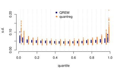
Figure 15: QR simulation #15: $\hat{\sigma}_{\hat{\beta}_{1}}$ for $q\in\{0.02,0.05,0.1,\ldots,0.95,0.98\}$ for $y\sim N(5+x,(0.1+0.5x)^{2})$.

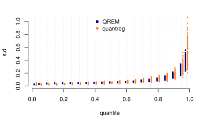
Figure 16: QR simulation #21: $\hat{\sigma}_{\hat{\beta}_{1}}$ for $q\in\{0.02,0.05,0.1,\ldots,0.95,0.98\}$ for $y=1-3x_{1}+2x_{2}+2x_{3}-x_{4}-2x_{5}+\epsilon_{i}$ and $\epsilon_{i}\sim LN(0,0.75)$.

We compared the estimated regression coefficients with those obtained from the quantreg package Koenker (2018), which uses a different estimation approach (namely, direct minimization of the loss function in 1.) Since our model is derived from the same loss function it is expected that the two methods would give similar estimates, and this is confirmed by our simulations. Indeed, the parameter estimates from both methods are nearly identical (the small differences are attributed to the chosen tolerance level of the computational methods and the fact that empirical quantiles are not uniquely defined). The variances of the regression parameter estimates from the two methods, however, are quite different. Recall that we obtain the asymptotic covariance of $\hat{\bm{\beta}}$ by using Bahadur’s representation, which requires the estimation the density of the residual $u_{i}$ at 0. To do that, we use kernel density estimation, as implemented in the KernSmooth package Wand (2015). See Deng and Wickham (2014) for a review of kernel density estimation packages. The quantreg package computes confidence intervals using the inversion of a rank test, per Koenker (1994). Figure 3 shows $\hat{\sigma}_{\hat{\beta}_{1}}$ for $q\in\{0.05,0.1,\ldots,0.95\}$, using QREM (blue squares, left), the bootstrap (dark-red triangle, middle), and quantreg (orange circles, right). The horizontal yellow lines above each quantile represent the true estimate of the standard deviation of $\hat{\beta}_{1}$, as obtained from the asymptotic Bahadur-type estimation using the true density of $u_{i}$ at 0. Our estimator has a smaller sampling variance across all scenarios and all quantiles. Figures 15 and 16 in Appendix A show the estimated standard deviations of $\hat{\beta}_{1}$ obtained from QREM and quantreg for scenarios 15 and 21, respectively. Again, the sampling variance of $\hat{\sigma}_{\hat{\beta}_{1}}$ obtained from QREM is smaller than the one from quantreg, and especially near the edges ($q<0.15$ and $q>0.85$.) These results show that while on average the coverage probability of the two methods is expected to be similar, the smaller variance obtained from the QREM procedure imply that results from this method are more stable and provide more reliable inference. The wider range of variance estimates obtained from quantreg imply that this method is much more likely to lack power or to be over-powered.

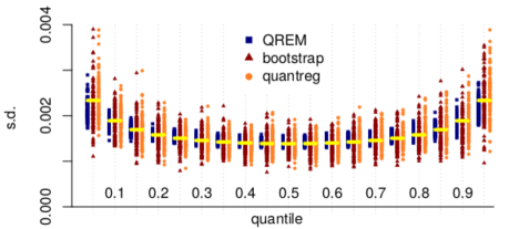
Figure 3: QR simulation: $\hat{\sigma}_{\hat{\beta}_{1}}$ for $q\in\{0.05,0.1,\ldots,0.95\}$ for $y\sim N(-3+x,0.1^{2})$.

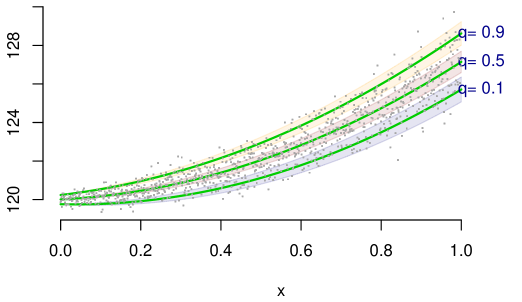
Figure 4: QR simulation - the 0.1, 0.5, and 0.9 quantiles with 90% confidence intervals, when the true model is $y\sim N(6x^{2}+x+120,(0.2+x)^{2})$.

We also simulated data in which the response depends on predictors in non-linear ways (simulations 23 and 24). For example, for simulation 23, in Figure 4 we show results when $y\sim N(6x^{2}+x+120,(0.2+x)^{2})$ so that the relation between the mean of $y$ and $x$ is a quadratic function, and the standard deviation increases linearly with $x$. The figure shows the 0.1, 0.5, and 0.9 quantiles with 90% confidence bands. For all values of $x$, the three quantile regression curves are significantly different from the each other. To assess goodness of fit, we use the quantile-quantile plot construction as described in Section 3. For example, Figure 5 shows the QQ plot for the predictor $x$ when $q=0.1$: on the left hand side, we fitted a linear model, $y\sim x$, and on the right hand side the fitted model is $y\sim x+x^{2}$ (the true model). The QQ plot suggests that, for the 10th percentile, the linear model is inadequate, while the quadratic one fits very well. The goodness of fit, as defined in Section 3, is is $G=1,135$ for the linear model, and $G=828$ for the quadratic model, again providing evidence that in this case a quadratic model provides a better fit.

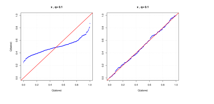
Figure 5: QR simulation - the true model is $y\sim N(6x^{2}+x+120,(0.2+x)^{2})$. Showing quantile-quantile plots for the linear predictor $x$ when fitting a linear (left) and the correct, quadratic model (right), for $q=0.1$.

It is possible that a model would fit well for certain quantiles, but not for others. The final example in this section demonstrates this point and shows an effective way to visualize multiple QQ-plots, when fitting the same quantile regression model for different $q$s. We simulated 10,000 points from a bivariate uniform distribution on $[0,1]\times[0,1]$ as our two predictors, $x_{1}$ and $x_{2}$, and generated the response using the interaction of the predictors, so that $y\sim N(4x_{1}x_{2},(0.1+0.2x_{1})^{2})$ (simulation 24 in the Appendix). For each $q\in(0.05,0.1,\ldots,0.9,0.95)$ we fitted two models - one additive, $y\sim x_{1}+x_{2}$, and one with an interaction term, $y\sim x_{1}+x_{2}+x_{1}x_{2}$. From each fitted model we obtained the theoretical and empirical quantiles, $Q_{q,t}(x_{1})$, and $Q_{q,e}(x_{1})$, respectively, with respect to $x_{1}$. Recall that under the correct model the plot of the theoretical versus empirical quantiles should lie close to the $45^{\circ}$ line. So, for a fixed $q$, and some $\xi_{1}$ in the range of $x_{1}$ we define $r_{q}(\xi_{1})=n_{q,e}(\xi_{1})/n_{q,t}(\xi_{1})$ where $n_{q,e}$ and $n_{q,t}$ are the numbers of empirical and theoretical quantiles that are smaller than $\xi_{1}$. An adequate model gives $r_{q}(\xi_{1})\approx 1$ for each value of $\xi_{1}$. For each $q$ we use $L$ (e.g., 20) equally spaced values in the range of $x_{1}$, denoted by $\xi_{1j}$, and obtain $r_{q}(\xi_{1j})$. We plot an array of rectangles with colors corresponding to the values of $r_{q}(\xi_{1j})$, so that the columns in the array correspond to the quantiles, and the rows to $\xi_{1j}$. This yields a heatmap, as depicted in Figure 6, to which refer as a ‘flat’ QQ plot, since for each $q$ we convert the two-dimensional QQ plot to a single column in the heatmap. Figure 6-A shows an ideal ‘flat’ QQ-plot. The interaction model fits very well for each $q$. In contrast, Figure 6-B shows that although the additive model suggests a good fit for values around $q=0.5$, it is inadequate for most $q$’s.

Figure 6: a ‘flat’ QQ plot for $q\in(0.05,0.1,\ldots,0.9,0.95)$, when the true model is $y\sim N(4x_{1}x_{2},(0.1+0.2x_{1})^{2})$. A: fitting the correct (interaction) model. B. Fitting an additive (incorrect) model, $y\sim x_{1}+x_{2}$.

Finally, we also simulated data from mixed models. In simulation 25 we generated a random samples of $100$ independent subjects, and each subject was observed at four time points. Within subject the observations were correlated. That is, we used a variance component model, where $y_{it}=2+x_{it}+u_{i}+\epsilon_{it}$, and the random effect, $u_{i}$, was distributed as $N(0,0.5^{2})$, and the random errors as $\epsilon_{it}\sim N(0,0.1^{2})$.

To obtain confidence intervals for the parameter estimates we used a bootstrap approach and fitted the QR model 1,000 times for each $q=\{0.1,\ldots,0.9\}$, each time drawing a random sample (with replacement) from the subjects. The parameter estimates and the bootstrap standard errors were very accurate for all deciles: the average bias for $\beta_{1}$ was 0.0008, and the 95% coverage probability was $0.95\pm 0.005$.

6 Case Studies

6.1 BMI and Microbiome Data

An operational taxonomic unit (OTU) is an operational definition used to classify groups of closely related organisms. OTUs have been the most commonly used units of microbial diversity, especially when analyzing small subunit 16S rRNA marker gene sequence datasets. In this case study we illustrate a quantile regression approach to the analysis of microbiome compositional covariates using BMI and OTU data from Wu et al. (2011). Bar et al. (2018) applied SEMMS (Scalable EMpirical Bayes Model Selection) with BMI as a continuous response with compositional OTU covariates, using the normal model and obtained the same four genera reported by the LASSO-based variable selection method in Lin et al. (2014) (Acidaminococcus, Alistipes, Allisonella, and Clostridium). Bar et al. (2018) also demonstrated the application of SEMMS using a categorical version of BMI with 3 levels: normal [18.5, 25) (n=30), overweight [25.5, 30) (n=25), and obese $\geq$30 (n=10) and found six bacteria associated with obesity relative to normal (Acidaminococcus, Alistipes, Allisonella, Butyricimonas, Clostridium, and Oxalobacter) and five with overweight relative to normal (Anaerofilum, Faecalibacterium, Oscillibacter, Turicibacter, and Veillonella). A logistic regression approach using SEMMS for the obese group (n=10) when the baseline consisted of the non-obese subjects (BMI$<$30, n=86) found five genera (Acidaminococcus, Alistipes, Allisonella, Dialister, and Dorea). The fact that Acidaminococcus, Alistipes, Allisonella, and Clostridium are a subset of the genera found to be associated with obese individuals but have no overlap with the ones associated with overweight suggest that different BMI levels are associated with different bacteria, and thus hint that quantile regression will give a more interpretable analysis than the conditional mean regression model.

Since microbiome abundance data is compositional, to apply our method directly, without changing the model to account for the sum constraint, we perform the log ratio transformation and replace the matrix $X$ with $X^{K}=\log(x_{ij}/x_{iK})$, where the $x_{iK}$ are replications of a reference bacteria genera. The data contains many zero counts, so Bar et al. (2018); Lin et al. (2014) replace them with 0.5 before converting the data to be in compositional form. As in Lin et al. (2014); Bar et al. (2018) we use a subset of 45 bacteria which had non-zero counts in at least 10% of the samples ($N=96$). The omitted genera have minimal contribution to the overall distribution of the proportions.

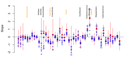
Figure 7: Mean-model estimates and their confidence intervals in red, and the quantile regression coefficients for $q=0.2,\ldots,0.8$ in blue (diamonds, where the increased size corresponds to larger $q$).

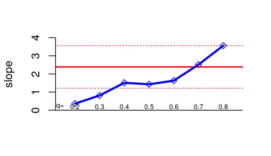
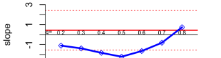
Figure 8: Mean-model estimates and their confidence intervals in red and quantile regression coefficients for $q=0.2,\ldots,0.8$ for Allisonella (top) and Gemella (bottom).

Figure 7 shows the mean-model estimates and their confidence intervals in red, and the quantile regression coefficients for $q=0.2,\ldots,0.8$ in blue (diamonds, where the size corresponds to $q$). This is done one OTU at a time with no adjustment for multiple testing. Most confidence intervals are quite large, and contain all the quantile regression estimates. The quantile regression analysis leads to a number of interesting points. For example in Figure 8, Allisonella has a strong mean effect ($\sim 2.5$) but even stronger quantile effect for $q=0.8$. Notice also that Gemella, Granulicatella, Anaerofustis have a small positive mean-effect estimate, but the estimates for the lower quantiles are negative and are outside the mean confidence interval. For some OTUs the effect for all quantiles has the same sign, maybe suggesting that these OTUs should be considered as significant even if the adjusted p-value for the mean effect is not sufficiently small. For example, Acidaminococcus, Megasphaera, Catenibacterium (all positive) and Alistipes, Clostridium, Oscillibacter (all negative) have a fairly small spread of quantile regression estimates, perhaps suggesting that they are in fact significant, even if their p-value after adjustment is not small enough.

The quantile regression results are consistent with the previous findings in the microbiome literature. The relative proportion of phylum Bacteroidetes (containing the Alistipes genus) to phylum Firmicutes (all other genera found) is lower in obese mice and humans than in lean subjects Ley et al. (2006). In Andoh et al. (2016) Gemella, Granulicatella were both found to be increased bacteria genera in obese people but not as a differential between lean and obese people, this is reflected in the quadratic behavior seen for Gemella in Figure 8. Furthermore, the family Veillonellaceae (containing the Acidaminococcus and Allisonella genera) are positively correlated to BMI Wu et al. (2011). The two additional genera found beyond Lin et al. (2014), Catenibacterium and Megamonas, have been found to be positively associated with BMI. Chiu et al. (2014) identify Megamonas as a genus that differentiates between low and high BMI in a Taiwanese population and Turnbaugh et al. (2009) found that the Catenibacterium genus increased diet-induced dysbiosis for high-fat and high-sugar diets in humanized gnotobiotic mice.

6.2 Daily Temperature Data

We demonstrate fitting a quantile regression mixed-model using our approach to daily temperature data from four U.S. cities (Chicago, Ithaca, Las Vegas, and San Francisco). Minimum and maximum temperatures (in Fahrenheit) from January 1, 1960 to December 31, 2010 were obtained from the National Oceanic and Atmospheric Administration website (https://www.noaa.gov/). We fit a model which allows for the temperature characteristics to change linearly over time, while accounting for the cyclical nature of temperatures. To allow for extra variability in the data in addition to between-days variability, we include a random intercept for each month of the year. Let $y_{ijk}$ denote the daily maximum (minimum) temperature in month $j$ and day $k$ of year $i$ and define $S_{k}=\sin(2\pi(k-11)/365-\pi/2)$, for $k=1,\ldots,365$ (or $366$), to represent the annual sinusoidal variation of daily temperatures, with a minimum at (approximately) the shortest day of the year in the northern hemisphere, December 21, and a maximum at around June 21. Our main objective is to estimate linear trends in temperatures over the 50 year period. For each city we fit six models with linear predictors of the form

$$\eta_{ijk}=\mu+\beta_{1}i+\beta_{2}S_{k}+v_{j}\,.$$

for the 10-th percentile, the mean, or the 90-th percentile of the daily minimum or maximum temperature, and where $v_{j}$, $j=1,\ldots,12$ is a (random) effect of month $j$. The lmer function Bates et al. (2015) was used to fit the parameters in each iteration of the EM algorithm (in the M-step.)

The estimates of $\beta_{1}$ from each model are summarized in Table 1 for all four cities. All cells with total temperature increase of more than 1 degree are statistically significant. For example, in San Francisco the minimum daily temperatures rose on average by only 0.1 degrees from 1960 to 2010, but the 90-th percentile of the maximum daily temperature increased by 4.7 degrees. The mean maximum daily temperatures increased by 3.4 degrees in those 50 years. In Las Vegas, on the other hand, the 90-th percentile of the maximum daily temperature increased by 1 degree, but the 10-th percentile of the minimum daily temperature increased by almost 9 degrees. In both Chicago and Las Vegas, the largest increase for both minimum and maximum daily temperatures has been to the 10-th percentile, which means that the 10% ‘cooler than usual for the time of year’ days were quite warmer in 2010 than in 1960.

	Chicago			Ithaca			Las Vegas			San Francisco
	Illinois			New York			Nevada			California
	10%	M	90%	10%	M	90%	10%	M	90%	10%	M	90%
min temp.	4.3	2.9	1.6	2.1	1.8	1.3	8.7	7.8	6.9	0.1	0.1	0.2
max temp.	1.9	1.2	0.3	1.1	1.2	1.5	2.0	1.5	1.0	2.5	3.4	4.7

Table 1: The total change in temperature from 1960-2009 in four U.S. cities. In each city we estimate the change in the minimum and maximum temperatures in terms of the 10-th percentile, the mean, and the 90-th percentile.

The fitted lines for the quantile regression models with $q=0.1,0,9$ are shown for the Las Vegas data for 1960-64 and 2006-10 in Figure 9. The sharp increase in minimum daily temperatures of approximately 8 degrees between 1960-4 and 2006-10 can be seen very clearly (top). Figure 10 shows the daily minimum and maximum temperatures for Chicago and San Francisco, from 1985-1990, as well as the fitted lines from our quantile regression for $q=0.1$ (blue) and $q=0.9$ (red). The plot shows that although both cities have cyclical patterns, their shapes are quite different. The mixed model in which the cyclical fixed effect is dominant and the random month-by-month intercept allows for deviations from the sinusoidal pattern seems to fit both patterns quite well. For Chicago, the sinusoidal shape is very clear, whereas in San Francisco the pattern is skewed with a sharp decline in temperatures in the fall and a slower incline starting in January. It looks like late-spring and summer in San Francisco are a lot more likely to have maximum temperature which are much higher than the mean-model predicts (black curve in the bottom-right plot), and the 90-th percentile seems much more informative.

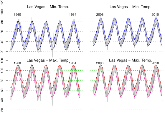
Figure 9: The fitted lines for the quantile regression models for Las Vegas for 1960-1964 (left) and 2006-2010 (right) with $q=0.1$ and $q=0.9$. The actual observations are shown in grey. Top: minimum daily temperature, bottom: maximum daily temperature.

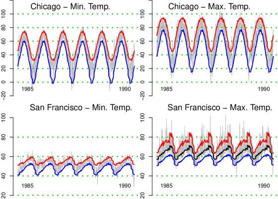
Figure 10: Daily minimum and maximum temperatures for Chicago and San Francisco, from 1985-1990. Fitted lines from our quantile regression for $q=0.1$ in blue and $q=0.9$ in red. For max. temperatures in San Francisco we show the fitted curve from the mean model in black.

To check the model fit, we produced QQ plots as demonstrated in the previous section. For Chicago, Ithaca, and Las Vegas, the plot for each predictor and each quantile (0.1 and 0.9) was along the diagonal, for both the minimum and maximum temperatures. See, for example, the QQ plot for the year predictor for the maximum temperatures in Las Vegas in Figure 11 on the left. However, for San Francisco, the QQ plots for the year variable exhibited a slightly curved pattern (Figure 11, right-hand side). Looking at the time-series plot (not shown here) we see that this could be due to a period of time (1984-1997) in which the percentage of especially high maximum temperatures in a single year was higher than usual.

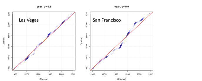
Figure 11: Quantile-quantile plot for the maximum temperatures in Las Vegas (left) and San Francisco (right), corresponding to the ‘year’ predictor, when fitting the quantile regression with $q=0.9$

Figure 12 shows the ‘flat’ QQ plot for the maximum temperature in San Francisco, for $q=0.1,0.2,\ldots,0.9$, with respect to the year predictor. Using the notation from the previous section, the range of $r_{q}(\xi_{year,j})$ is $0.88-1.26$. Although most of the values are close to 1, the model does not fit the data for San Francisco as well as for the other three cities (not shown here). Note that the goodness of fit of the model varies by the selected quantile, $q$. In particular, the worst fit is for the median, where, around 1970, the predicted values are 1.26 higher than the observed median temperatures.

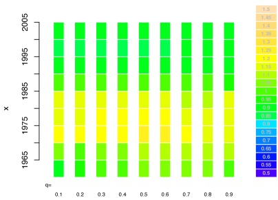
Figure 12: A ‘flat’ Quantile-quantile plot for the maximum temperatures in San Francisco with respect to the ‘year’ predictor, for $q=0.1,0.2,\ldots,0.9$

6.3 Frailty QR Model – Emergency Department Data

The National Center for Health Statistics, Centers for Disease Control and Prevention conducts annual surveys to measure nationwide health care utilization. We use the 2006 NHAMCS (National Hospital Ambulatory Medical Care Survey) data to demonstrate fitting quantile regression models with random effects to survival-type data. In this case, the length of visit (LOV, given in minutes) while in a hospital emergency department (ED) is considered the ‘survival’ time, and we define the normalized response $y=\log_{60}(LOV+1)$. We filter the data and remove hospitals with fewer than 70 visits, which results in 21,262 ED visit records from 230 hospitals.

First, we fit a fixed-effect model which includes nine predictors of interest: Sex, Race (white, black, other), Age (standardized to a $[0,1]$ range), Region (northeast, midwest, south, and west), Metropolitan area (yes/no), Payment Type (Private, Government/Employer, Self, and Other), Arrival Time (8AM-8PM or 8PM-8AM), the Day of the Week, and a binary variable (Recent Visit) to indicate whether the patient has been discharged from a hospital in the last 7 days, or from an ED within the last 72 hours. We fit a QR (fixed-effect) model for $q=0.025,0.05,0.075,\ldots,0.975$. Then, we fit the frailty model for the same quantiles using the same nine predictors, plus the Hospital as a random effect, and check whether the coefficients of the fixed effects change when we account for the correlation between patients within a hospital.

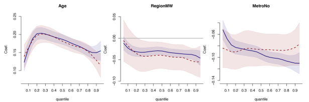
Figure 13: ED data – quantile regression coefficients with 95% point-wise confidence intervals, from left to right, for Age, Region (=midwest, where northeast is the baseline), and Metro (=No, where Yes is the baseline). The blue, solid line is the for the fixed effect model coefficients, and the red, dashed line is for the mixed model coefficients.

Figure 13 shows the regression coefficients, from left to right, for Age, Region (=midwest, where northeast is the baseline), and Metro (=No, where Yes is the baseline). For these variables, the coefficients are remain approximately the same when we add the Hospital random effect. Age has a positive effect for all quantiles, and the smallest difference in LOV due to age is for the patients who are discharged quickly from the ED, or those who stay at the ED the longest. Generally, ED patients in the northeast have longer visits than the ones in the midwest (except for those who are discharged quickly). Similarly, ED patients in a metropolitan area stay significantly longer than in rural area hospitals. The Arrival Time and Day of Week variables are also similar whether we include the hospital random effect or not (no shown here.) Arriving at an ED on Monday results in a longer wait compared with Sunday (except for patients who are discharged quickly), but the difference between other weekdays and the weekend is less significant for most quantiles. Arriving at night means a longer stay only for the patients who end up staying the longest (the upper 20-th percentile in the fixed effect model but no significant difference in the mixed model), but among patients who are discharged relatively quickly ($q\leq 0.2$) arriving at night actually corresponds to a shorter stay, as compared with day-time arrival.

Figure 14 shows that accounting for within-hospital correlation yields very different results compared with the fixed-effect model. According to the fixed effect model one might conclude that there is a significant difference between blacks and whites (left panel) and between people with private health insurance versus people whose medical bill is ‘Other’ (namely, not Private, Medicare, Medicaid/SCHIP, Worker’s Compensation, or Self pay), for patients who are not discharged quickly, i.e., for $q>0.2$. Similarly, from the fixed effect model one might conclude that among those who are not discharged quickly, a recent visit to a hospital or an ED will result in longer stays (for $q>0.35$). However, the results from the mixed model suggest that these differences can be explained by variation between hospitals, while, within a hospital there is no significant difference in the length of visit between black and white people, or between people with private insurance and people who ‘other’ pay.

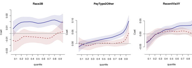
Figure 14: ED data – quantile regression coefficients with 95% point-wise confidence intervals, for Race=Black (left, with White as baseline), Pay Type (center, for ‘Other’ source of payment versus ‘Private’), and Recent Visit (for Yes, versus the No reference.) The blue, solid line is the for the fixed effect model coefficients, and the red, dashed line is for the mixed model coefficients.

7 Discussion

The EM formulation introduced in this paper for fitting quantile regression models offers a few advantages over existing methods stemming from the fact that the M-step involves a mean regression via weighted least squares. This formulation suggests an approach to fitting mixed effects quantile regression models that can be justified as a GAM algorithm. We see several possibilities for interesting applications and extensions, such as quantile regression with autoregressive (or ARMA) errors, and spatial models that use the mixed models framework to specify the correlation structure. Another extension is to variable selection for the ‘large p’ scenario in which the variables are selected based on their association with quantiles, rather than a mean response, by modifying the methodology developed in Bar et al. (2018).

Appendix A Appendix

A.1 Proofs

Proof of Proposition 1:
First note that the check loss function (1) can be written as

$$\rho_{q}(u_{i})=\frac{1}{2}\left[|u_{i}|+(2q-1)u_{i}\right]\,,\mbox{ so we can write:}$$

$$e^{-2\rho_{q}(u_{i})}=e^{-(2q-1)u_{i}}e^{-|u_{i}|}\,.$$

The marginal distribution of $u$ is denoted by $h(u)$, where

$$h(u) = \int_{0}^{\infty}\frac{1}{\sqrt{2\pi\lambda}}\exp\left[-\frac{(u-(1-2q)\lambda)^{2}}{2\lambda}\right]\cdot 2q(1-q)\exp\left[-2q(1-q)\lambda\right]d\lambda$$

$$= 2q(1-q)\int_{0}^{\infty}\frac{1}{\sqrt{2\pi\lambda}}\exp\left[-\frac{u^{2}-2u(1-2q)\lambda+(1-2q)^{2}\lambda^{2}+4q(1-q)\lambda^{2}}{2\lambda}\right]d\lambda$$

$$= 2q(1-q)\int_{0}^{\infty}\frac{1}{\sqrt{2\pi\lambda}}\exp\left[-\frac{u^{2}-2u\lambda+\lambda^{2}(1-4q+4q^{2}+4q-4q^{2})+4qu\lambda}{2\lambda}\right]d\lambda$$

$$= 2q(1-q)\int_{0}^{\infty}\frac{1}{\sqrt{2\pi\lambda}}\exp\left[-\frac{u^{2}-2u\lambda+\lambda^{2}}{2\lambda}-2qu\right]d\lambda$$

$$= 2q(1-q)\int_{0}^{\infty}\frac{1}{\sqrt{2\pi\lambda}}\exp\left[-\frac{u^{2}/\lambda-2u+\lambda}{2}-2qu\right]d\lambda$$

$$= 2q(1-q)\int_{0}^{\infty}\frac{1}{\sqrt{2\pi\lambda}}\exp\left[-\frac{u^{2}/\lambda+\lambda}{2}-(2q-1)u)\right]d\lambda$$

$$= 2q(1-q)e^{-(2q-1)u}\int_{0}^{\infty}\frac{1}{\sqrt{2\pi\lambda}}\exp\left\{-\frac{1}{2}(\lambda+u^{2}/\lambda)\right\}d\lambda$$

From Polson and Scott (2012) and formula 12 on page 368 of Gradshteyn and Ryzhik (2014) (with $y=x/2$ and $\nu=.5$) we have that

$$e^{-|u|}=\int_{0}^{\infty}\frac{1}{\sqrt{2\pi\lambda}}\exp\left\{-\frac{1}{2}(\lambda+u^{2}/\lambda)\right\}d\lambda\,,$$

It follows that,

$$h(u) = 2q(1-q)\exp\{-[(2q-1)u+|u|]\}=2q(1-q)\exp[-2\rho_{q}(u)]\,.$$

Proof of Proposition 4:
We denoted the scaled, binary-valued QR residuals by $\mathbf{c}=sgn(Y-X^{T}\bm{\beta}_{q})-(1-2q)\mathbf{1}$. We found the WLS solution from the M-step:

$$\bm{\beta}_{q}=(X^{T}\Lambda^{-1}X)^{-1}X^{T}\Lambda^{-1}\left[Y-(1-2q)\bm{\lambda}\right].$$

Multiplying both sides by $(X^{T}\Lambda^{-1}X)^{-1}$ we get

$$(X^{T}\Lambda^{-1}X)\bm{\beta}_{q}=X^{T}\Lambda^{-1}\left[Y-(1-2q)\bm{\lambda}\right]$$

and rearranging terms we get

$$X^{T}\Lambda^{-1}(Y-X^{T}\bm{\beta}_{q}) = (1-2q)X^{T}\Lambda^{-1}\bm{\lambda}$$

$$= (1-2q)X^{T}\mathbf{1}\,.$$

Expressing $Y-X^{T}\bm{\beta}_{q}$ as $\Lambda\cdot sgn(Y-X^{T}\bm{\beta}_{q})$ we get

$$X^{T}\Lambda^{-1}[\Lambda\cdot sgn(Y-X^{T}\bm{\beta}_{q})] = (1-2q)X^{T}\mathbf{1}$$

so, $X^{T}\mathbf{c}=\mathbf{0}$.

A.2 Conditions for consistency of the QR estimator

Let the $q$th conditional quantile function of $Y|\mathbf{X}$ be $Q_{Y}(q|\mathbf{X})$. Per (Koenker et al., 2005, Section 4.1.2), for the quantile regression estimator $\hat{\bm{\beta}}_{q}$ to be consistent, the following conditions have to hold:

1. There exists $d>0$ such that

   $$\underset{n\rightarrow\infty}{\lim\inf}\underset{\|u\|=1}{\inf}n^{-1}\sum I(|\mathbf{x}_{i}^{\prime}u|<d)=0\,.$$

2. There exists $D>0$ such that

   $$\underset{n\rightarrow\infty}{\lim\sup}\underset{\|u\|=1}{\sup}n^{-1}\sum(\mathbf{x}_{i}^{\prime}u)^{2}\leq D\,.$$

A.3 Simulation Scenarios

No.	Description	Model for the response, $y$	Error distribution
1	Intercept only	$3$	$N(0,0.25^{2})$
2-11	Simple linear model	$5-x$	$N(0,\sigma^{2})$, $\sigma\in\{0.1,0.2,\ldots,1\}$
12	Two predictors	$1-3x_{1}+2x_{2}$	$N(0,0.1^{2})$
13	Five predictors	$1-3x_{1}+2x_{2}+2x_{3}-x_{4}-2x_{5}$	$N(0,0.1^{2})$
14	s.d. increases linearly	$3+2x$	$N(0,(0.1+0.2x)^{2})$
15	s.d. increases linearly	$5+x$	$N(0,(0.1+0.5x)^{2})$
16	s.d. increases linearly	$3+0.5x$	$N(0,(0.5+0.7x)^{2})$
17	Polynomially increasing s.d.	$1-2x$	$N(0,(0.1+0.2x^{3})^{2})$
18	Linearly decreasing s.d.	$7+3x$	$N(0,(1-0.5x)^{2})$
19	Intercept only	$5$	$LN(0,0.75)$
20	Simple linear model	$3-x$	$LN(0,0.75)$
21	Five predictors	$1-3x_{1}+2x_{2}+2x_{3}-x_{4}-2x_{5}$	$LN(0,0.75)$
22	Linearly increasing (log) s.d.	$2-2x$	$LN(0,0.5+0.5x)$
23	Quadratic, increasing variance	$6x^{2}+x+120$	$N(0,(0.2+x)^{2})$
24	Interaction, increasing variance	$4x_{1}x_{2}$	$N(0,(0.1+0.2x_{1})^{2})$
25	Mixed model	$2+x+z^{\prime}u$	$u\sim N(0,0.5^{2})$, $e\sim N(0,0.1^{2})$

Table 2: Simulation scenarios. In simulations 1-11, 14-17, and 24 the predictors were drawn uniformly from $(0,1)$. In simulation 12 $x_{1}\sim U(0,1)$ and $x_{2}\sim U(-3,3)$. In simulations 13, 18-22 the predictors were drawn uniformly from $(-1,1)$ and in simulation 23, from $(-5,5)$. In simulation 25, $x_{it}\sim N(t/4,0.1^{2})$, for $t=1,2,3,4$.

References

- Albert and Chib (1993) Albert, J. H. and S. Chib (1993). Bayesian analysis of binary and polychotomous response data. Journal of the American Statistical Association 88(422), 669–679.
- Andoh et al. (2016) Andoh, A., A. Nishida, K. Takahashi, O. Inatomi, H. Imaeda, S. Bamba, K. Kito, M. Sugimoto, and T. Kobayashi (2016). Comparison of the gut microbial community between obese and lean peoples using 16s gene sequencing in a japanese population. Journal of clinical biochemistry and nutrition, 15–152.
- Bahadur (1966) Bahadur, R. R. (1966, 06). A note on quantiles in large samples. Ann. Math. Statist. 37(3), 577–580.
- Bar et al. (2018) Bar, H., J. Booth, and M. T. Wells (2018). A scalable empirical bayes approach to variable selection in generalized linear models. arXiv preprint arXiv:1803.09735.
- Bates et al. (2015) Bates, D., M. Mächler, B. Bolker, and S. Walker (2015). Fitting linear mixed-effects models using lme4. Journal of Statistical Software 67(1), 1–48.
- Chiu et al. (2014) Chiu, C.-M., W.-C. Huang, S.-L. Weng, H.-C. Tseng, C. Liang, W.-C. Wang, T. Yang, T.-L. Yang, C.-T. Weng, T.-H. Chang, et al. (2014). Systematic analysis of the association between gut flora and obesity through high-throughput sequencing and bioinformatics approaches. BioMed Research International 2014.
- Dempster et al. (1977) Dempster, A. P., N. M. Laird, and D. B. Rubin (1977). Maximum likelihood from incomplete data via the EM algorithm. Journal Of The Royal Statistical Society, Series B 39(1), 1–38.
- Deng and Wickham (2014) Deng, H. and H. Wickham (2014). Density estimation in R. https://vita.had.co.nz/papers/density-estimation.pdf.
- Galarza et al. (2017) Galarza, C. E., V. H. Lachos, and D. Bandyopadhyay (2017). Quantile regression in linear mixed models: a stochastic approximation em approach. Statistics and its interface 10 3, 471–482.
- Geraci and Bottai (2007) Geraci, M. and M. Bottai (2007). Quantile regression for longitudinal data using the asymmetric Laplace distribution. Biostatistics 8(1), 140–154.
- Geraci and Bottai (2014) Geraci, M. and M. Bottai (2014). Linear quantile mixed models. Statistics and Computing 24(3), 461–479.
- Good (1953) Good, I. (1953). The population frequencies of species and the estimation of population parameters. Biometrika 40, 237–260.
- Gradshteyn and Ryzhik (2014) Gradshteyn, I. and I. Ryzhik (2014). Table of integrals, series, and products. Academic Press.
- Gunawardana and Byrne (2005) Gunawardana, A. and W. Byrne (2005, December). Convergence theorems for generalized alternating minimization procedures. J. Mach. Learn. Res. 6, 2049–2073.
- Hunter and Lange (2000) Hunter, D. R. and K. Lange (2000). Quantile regression via an MM algorithm. J. Comput. Graphical Stat, 60–77.
- Kocherginsky et al. (2005) Kocherginsky, M., X. He, and Y. Mu (2005). Practical confidence intervals for regression quantiles. Journal of Computational and Graphical Statistics 14(1), 41–55.
- Koenker (1994) Koenker, R. (1994). Confidence intervals for regression quantiles. Springer.
- Koenker (2018) Koenker, R. (2018). quantreg: Quantile Regression. R package version 5.38.
- Koenker and Bassett (1978) Koenker, R. and G. J. Bassett (1978). Regression quantiles. Econometrica 46(1), 33–50.
- Koenker et al. (2005) Koenker, R., A. Chesher, and M. Jackson (2005). Quantile Regression. Econometric Society Monographs. Cambridge University Press.
- Koenker and Hallock (2001) Koenker, R. and K. Hallock (2001). Quantile regression an introduction. Journal of Economic Perspectives 15(4), 43–56.
- Koenker and D’Orey (1987) Koenker, R. W. and V. D’Orey (1987). Algorithm as 229: Computing regression quantiles. Journal of the Royal Statistical Society. Series C (Applied Statistics) 36, 383–393.
- Kozubowski and Podgorski (2000) Kozubowski, T. and K. Podgorski (2000). Asymmetric laplace distributions. Mathematical Scientist 25(1), 37–46.
- Kozumi and Kobayashi (2011) Kozumi, H. and G. Kobayashi (2011). Gibbs sampling methods for bayesian quantile regression. Journal of statistical computation and simulation 81(11), 1565–1578.
- Ley et al. (2006) Ley, R. E., P. J. Turnbaugh, S. Klein, and J. I. Gordon (2006). Microbial ecology: human gut microbes associated with obesity. Nature 444, 1022–1023.
- Lin et al. (2014) Lin, W., P. Shi, R. Feng, and H. Li (2014). Variable selection in regression with compositional covariates. Biometrika 101(4), 785–797.
- McNeil et al. (2005) McNeil, A., R. Frey, and P. Embrechts (2005). Quantitative Risk Management: Concepts, Techniques and Tools. Princeton University Press.
- Polson and Scott (2012) Polson, N. G. and J. G. Scott (2012, 12). On the half-cauchy prior for a global scale parameter. Bayesian Analysis 7(4), 887–902.
- Portnoy and Koenker (1997) Portnoy, S. and R. Koenker (1997). The gaussian hare and the laplacian tortoise: computability of squared-error versus absolute-error estimators. Statistical Science 12, 279–300.
- R Core Team (2018) R Core Team (2018). R: A Language and Environment for Statistical Computing. Vienna, Austria: R Foundation for Statistical Computing.
- Turnbaugh et al. (2009) Turnbaugh, P. J., V. K. Ridaura, J. J. Faith, F. E. Rey, R. Knight, and J. I. Gordon (2009). The effect of diet on the human gut microbiome: a metagenomic analysis in humanized gnotobiotic mice. Science Translational Medicine 1, 6ra14–6ra14.
- Wand (2015) Wand, M. (2015). KernSmooth: Functions for Kernel Smoothing Supporting Wand & Jones (1995). R package version 2.23-15.
- Wu et al. (2011) Wu, G. D., J. Chen, C. Hoffmann, K. Bittinger, Y.-Y. Chen, S. A. Keilbaugh, M. Bewtra, D. Knights, W. A. Walters, R. Knight, et al. (2011). Linking long-term dietary patterns with gut microbial enterotypes. Science 334, 105–108.
- Yu and Moyeed (2001) Yu, K. and R. Moyeed (2001). Bayesian quantile regression. Statistics and Probability Letters 54(4), 437–447.