Gravitational antiscreening in stellar interiors

Abstract

A new class of relativistic stellar structure equations which include the effects of an energy-dependent Newton coupling is presented. Significant modifications in the mass-radius relation for neutron stars are possible only if the running of the Newton coupling due to quantum gravity occurs at low energies. A new Buchdahl limit is derived and its physical implications are discussed. In particular, sub-Planckian self-gravitating objects with arbitrarily small radii are possible.

1 Introduction

One of the most important issues in modern astrophysics is to understand the fate of stars undergoing a gravitational collapse. It is believed that when the energy density of the collapsing star reaches Planckian scales, quantum effects will halt the collapse. The details of this mechanism depend on the theory of quantum gravity at hand and, in recent years, various scenarios have been put forward (see Ref. [1] for a review).

Over the past decades, Asymptotically Safe Gravity has emerged as a promising approach to obtain a consistent and predictive theory of quantum gravity. The key ingredient is the existence of a non-Gaussian fixed-point, acting as an ultraviolet (UV) attractor for the gravitational renormalization group flow. The possibility of quantizing gravity along these lines was first suggested by Weinberg in his seminal study in $d=2+\epsilon$ dimensions [2], but at that time this fixed point was not accessible in $d=4$ dimensions due to its non-perturbative character. After the introduction of the functional renormalization group equation for the effective average action [3, 4], a systematic investigation of the phase diagram of gravity has become possible. The initial analyses based on the simple Einstein-Hilbert truncation [5] have been extensively generalized by the inclusion of higher-derivatives operators [6, 7, 8, 9, 10, 11, 12, 13] and matter fields [14, 15, 16, 17, 18, 19, 20, 21, 22]. The presence of a non-Gaussian fixed point has further been tested in unimodular-gravity settings [23, 24, 25, 26] and for the case of spacetimes carrying a foliation structure [27, 28, 29, 30, 31, 32]. Beyond corroborating the existence of the non-Gaussian fixed point, all of these investigations support the conclusion that the dimension of the UV critical manifold is finite [33, 34].

One of the key features of the Asymptotic Safety scenario for quantum gravity is the anti-screening of the gravitational interaction at short distances. In fact, the existence of a non-trivial fixed point for the dimensionless Newton coupling, $g(k)=G(k)\,k^{2}$, implies that the dimensionful Newton coupling vanishes at high energies, $G(k\to\infty)\to 0$. Implications of this anti-screening behaviour for the structure of black holes have appeared in Refs. [35, 36, 37, 38, 39, 40, 41, 42, 43, 44, 45, 46, 47, 48], while consequences for the physics of the Early Universe have been studied in Refs. [49, 50, 51, 52, 53, 54, 55, 56, 57, 58, 59, 60, 61, 62, 63] (see Ref. [64] for a review).

The Asymptotic Safety mechanism can be understood in simple physical terms. Assuming that, in the large-distance limit, the leading quantum effects can be described by quantizing the linear fluctuations of the metric, one obtains a free field theory in a curved background spacetime whose elementary quanta, the gravitons, carry energy and momentum. The vacuum of this theory is thereby populated by virtual graviton pairs, and a test body will become “dressed” by a cloud of virtual gravitons surrounding it. Whereas quantum fluctuations screen external charges in QED, they have an antiscreening effect on external test masses in quantum gravity. As a consequence, the Newton constant becomes a density-dependent quantity which is smaller at shorter distances. This behavior is similar to the running of the non-Abelian gauge coupling in Yang-Mills theories, for which the vacuum turns out to be “paramagnetic" at large distances [65, 66].

As proposed by Markov and Mukhanov [67], a way to consistently incorporate the antiscreening character of the gravitational interaction in Cosmology consists of introducing an energy-dependent Newton coupling as an effective multiplicative coupling between matter and geometry. In this work, we extend this formalism to study spherically symmetric field configurations. In particular we derive a modified Tolman-Oppenheimer-Volkoff (TOV) equation [68, 69, 70], and discuss its physical consequences. The specific scaling of the running gravitational coupling derived from the renormalization group analysis is then used at a later stage as an external input to work out explicit results, but different scenarios for quantum gravity could also be considered (see, e.g., Refs. [71, 72, 73, 74, 75, 76, 77, 78, 79, 80, 81]).

As expected, if quantum gravity sets in at Planckian scales, corrections to the mass-radius relation for macroscopic astrophysical sources are negligible. Clearly, these corrections would become phenomenologically more relevant in scenarios where the scale of quantum gravity is significantly lower than the Planck scale, but we do not pursue this line in the present work. The most significant consequence of the energy dependence of the gravitational interaction is a modification of the Buchdahl bound [82] for Planckian-size objects. Specifically, due to the antiscreening character of gravity at short distances, the Buchdahl limit deviates from the classical one at Planckian scales and matches the Schwarzschild limit at a critical radius $R_{\ast}^{\mathrm{crit}}\sim 0.37\,L_{\mathrm{Pl}}$, with $L_{\mathrm{Pl}}$ being the Planck length. Above this critical point, i.e., for $R\gtrsim R_{\ast}^{\mathrm{crit}}$, the formation of Planckian stars of compactness beyond the classical Buchdahl limit and positive central pressure is possible. These Planckian-size stars are characterized by a radius extremely close to the Schwarzschild radius and, as a consequence, they would appear dark to distant observers. These objects thus match the idea of quasi-black-holes introduced in Refs. [83, 84] in the context of semi-classical gravity. Below the critical point $R_{\ast}^{\mathrm{crit}}$, the quantum-improved Buchdahl limit undergoes a further deviation, indicating a possible transition to a regime where the internal structure of stars is dominated by quantum-gravity fluctuations. In this regime, the existence of stars with positive isotropic internal pressure is more restricted, but the formation of horizonless astrophysical objects with arbitrarily small radii is still possible.

The plan of the paper is the following. In Sect. 2, we review the TOV equation in General Relativity. The field equations in the Markov-Mukhanov formalism are obtained in Sect. 3, whereas the derivation of the improved TOV equation is reported in Sect. 4. This equation is solved for a polytropic equation of state in Sect. 5, and the corresponding modified mass-radius relation is discussed. The effects on the Buchdahl limit for uniform stars are studied in Sect. 6. Finally, in Sect. 7 we summarize our findings.

2 TOV equation in Einstein gravity

In this section, we review the derivation of the classical TOV equation in General Relativity. This will serve to highlight the differences with respect to the case of an energy dependent coupling in the next section.

A static and spherically symmetric astrophysical system, such as a star, is described by a metric of the form

$$\mbox{${\rm d}$}s^{2}=c^{2}\,e^{\nu(r)}\,\mbox{${\rm d}$}t^{2}-e^{\lambda(r)}\,\mbox{${\rm d}$}r^{2}-r^{2}\left(\mbox{${\rm d}$}\theta^{2}+\sin^{2}\theta\,\mbox{${\rm d}$}\phi^{2}\right)\ .$$ (2.1)

The functions $\lambda(r)$ and $\nu(r)$ are determined by the internal structure of the star, specifically its composition and the matter distribution in its interior. A star can be modeled as a self-gravitating object made of a perfect fluid, with proper energy density $\epsilon=\epsilon(r)$ and hydrostatic pressure given by an equation of state (EoS) $p=p(\epsilon)$. The energy-momentum tensor reads

$$T_{\mu\nu}=\left[\epsilon+p(\epsilon)\right]c^{-2}\,u_{\mu}\,u_{\nu}-p(\epsilon)\,g_{\mu\nu}\ .$$ (2.2)

Replacing Eq. (2.1) and (2.2) into the Einstein equations yields [70]

$$G^{0}_{\ 0} \equiv e^{-\lambda}\left(\frac{\lambda^{\prime}}{r}-\frac{1}{r^{2}}\right)+\frac{1}{r^{2}}=\kappa\,\epsilon$$ (2.3)

$$G^{1}_{\ 1} \equiv -e^{-\lambda}\left(\frac{\nu^{\prime}}{r}+\frac{1}{r^{2}}\right)+\frac{1}{r^{2}}=-\kappa\,p$$ (2.4)

$$G^{2}_{\ 2} \equiv -e^{-\lambda}\left[\frac{\nu^{\prime\prime}}{2}+\frac{(\nu^{\prime})^{2}}{4}-\frac{\nu^{\prime}\,\lambda^{\prime}}{4}+\frac{\nu^{\prime}-\lambda^{\prime}}{2\,r}\right]=-\kappa\,p\ ,$$ (2.5)

where $f^{\prime}=\partial_{r}f$ for any function $f$, $\kappa=8\pi G_{0}/c^{4}$, and the gravitational coupling is the constant $G_{0}$. Since $\kappa$ is a constant, the conservation equation $\nabla_{\mu}G^{\mu}_{\ \nu}=\kappa\,\nabla_{\mu}T^{\mu}_{\ \nu}=0$ reduce to the only non-trivial condition

$$\nabla_{\mu}T^{\mu}_{\ 1}\equiv-p^{\prime}(r)-\frac{\nu^{\prime}(r)}{2}\left(\epsilon+p\right)=0\ .$$ (2.6)

Likewise, from Eq. (2.3), one obtains

$$e^{-\lambda}=1-\frac{2\,G_{0}\,M(r)}{c^{2}\,r}\ ,$$ (2.7)

where the mass function

$$M(r)=\frac{4\,\pi}{c^{2}}\int_{0}^{r}\epsilon(x)\,x^{2}\,\mbox{${\rm d}$}x$$ (2.8)

is such that the total mass of a star of radius $R_{\ast}$ is given by $M_{\ast}=M(R_{\ast})$. This mass coincides with the Arnowitt-Deser-Misner (ADM) mass [85] of the system.

The classical TOV equation [68, 69, 70] is finally obtained by combining Eqs. (2.4) and (2.6),

$$p^{\prime}(r)=-\left[p(r)+\epsilon(r)\right]\frac{G_{0}}{c^{2}\,r^{2}}\left[M(r)+\frac{4\,\pi\,r^{3}}{c^{2}}\,p(r)\right]\left[1-\frac{2\,G_{0}\,M(r)}{c^{2}\,r}\right]^{-1}\ ,$$ (2.9)

and reduces to the Newtonian equation of hydrostatic equilibrium in the non-relativistic limit, $c\to\infty$.

The TOV equation (2.9) and the relation (2.8) for the mass function are the equations governing the hydrostatic equilibrium for a self-gravitating spherically symmetric object. Once an EoS is specified, the TOV equation can be solved in order to determine the radial variation of the internal pressure $p=p(r)$ in a star interior.

3 Field equations in the Markov-Mukhanov formalism

We next consider the case in which matter couples with gravity via an energy dependent coupling. In order to derive the corresponding effective field equations, we follow the Markov-Mukhanov formalism [67], which was originally introduced in order to study a particular case in which the energy-dependent effective Newton coupling was assumed to vanish at short distances. Although the antiscreening character of gravity was introduced in Ref. [67] as an ad hoc assumption, it turns out to be realized if gravity is asymptotically safe [86], i.e., if the gravitational RG flow attains an interacting fixed point at high energies.

The starting point is a fluid whose gravitational dynamics is governed by the action

$$S=\frac{1}{2\kappa}\int\mbox{${\rm d}$}^{4}x\,\sqrt{-g}\left[R+2\,\chi(\epsilon)\,\mathcal{L}\right]\ ,$$ (3.1)

where $\mathcal{L}=-\epsilon$ is the matter Lagrangian [87] and $\epsilon$ is again the proper energy density of the fluid. The function $\chi=\chi(\epsilon)$ is an effective multiplicative coupling encoding the way matter interacts with gravity. The metric variation of the matter part of the Lagrangian yields

$$\frac{1}{\sqrt{-g}}\,\delta\left(2\,\sqrt{-g}\,\chi\,\epsilon\right)=2\left(\epsilon\,\frac{\partial\chi}{\partial\epsilon}+\chi\right)\delta\epsilon-\chi\,\epsilon\,g_{\mu\nu}\,\delta g^{\mu\nu}\ .$$ (3.2)

Here, the variation $\delta\epsilon$ is given by

$$\delta\epsilon=\frac{1}{2}\left[\epsilon+p(\epsilon)\right]\left(g_{\mu\nu}-c^{-2}u_{\mu}\,u_{\nu}\right)\delta g^{\mu\nu}\ ,$$ (3.3)

as recalled in Appendix A. Upon varying the action (3.1) with respect to the metric, we obtain the modified Einstein equations

$$R_{\mu\nu}-\frac{1}{2}\,R\,g_{\mu\nu}=\Lambda_{\mu\nu}\ ,$$ (3.4)

where $\Lambda_{\mu\nu}$ is the effective energy-momentum tensor

$$\Lambda_{\mu\nu}\equiv\left(\epsilon\,\frac{\partial\chi}{\partial\epsilon}+\chi\right)T_{\mu\nu}-\epsilon^{2}\,\frac{\partial\chi}{\partial\epsilon}\,g_{\mu\nu}\ .$$ (3.5)

We see that the matter fields, whose energy-momentum tensor $T_{\mu\nu}$ is given by Eq. (2.2), couple to gravity via the effective Newton coupling

$$G_{\mathrm{eff}}(\epsilon)\equiv\frac{c^{4}}{8\,\pi}\,\frac{\partial(\epsilon\,\chi)}{\partial\epsilon}\ .$$ (3.6)

In addition, the variation of the action (3.1) generates an effective cosmological constant

$$\Lambda_{\mathrm{eff}}(\epsilon)=-\epsilon^{2}\,\frac{\partial\chi}{\partial\epsilon}\ .$$ (3.7)

One should further note that consistency with the Bianchi identity demands that $\nabla_{\mu}\Lambda^{\mu\nu}=0$ and, on considering the explicit expression (2.2) of the matter energy-momentum tensor, it implies

$$\nabla_{\mu}\Lambda^{\mu\nu}=\frac{\partial(\epsilon\,\chi)}{\partial\epsilon}\,\nabla_{\mu}T^{\mu\nu}+\frac{\partial^{2}(\epsilon\,\chi)}{\partial\epsilon^{2}}\,(\epsilon+p)\left(c^{-2}u^{\mu}\,u^{\nu}-g^{\mu\nu}\right)(\partial_{\mu}\epsilon)=0\ .$$ (3.8)

This constraint is satisfied if the usual conservation equation $\nabla_{\mu}T^{\mu\nu}=0$ holds, along with (at least) one of the following conditions:

1. The quantity $(\epsilon\,\chi)$ is a linear function of the energy density:

   $$\frac{\partial^{2}(\epsilon\,\chi)}{\partial\epsilon^{2}}=0\ .$$ (3.9)

   In this case we must have $\chi=\chi_{0}+\frac{\chi_{1}}{\epsilon}$, which implies that $\chi\to\chi_{0}$ when $\epsilon\to\infty$. Of course, a regular low energy limit ($\epsilon\to 0$) requires $\chi_{1}=0$, and one is left with the standard general relativistic case upon identifying $\chi_{0}\equiv\kappa$ (see Eq. (3.6)).

2. The energy density and pressure satisfy the vacuum equation of state:

   $$\epsilon+p=0\ ,$$ (3.10)

   meaning that the energy-momentum tensor is trivially conserved in de Sitter spacetimes, independently of the effective gravitational coupling $\chi$.

3. The gradient of the energy density is proportional to the fluid’s four-velocity:

   $$\left(c^{-2}\,u^{\mu}\,u^{\nu}-g^{\mu\nu}\right)(\partial_{\mu}\epsilon)=0\ .$$ (3.11)

   This case could be relevant for cosmology since it implies that the energy-momentum tensor of a homogeneous fluid sourcing the Friedmann-Lemaitre-Robertson-Walker spacetime is generally conserved for any choice of $\chi$.

Conversely, if none of the above conditions holds, one cannot have $\nabla_{\mu}T^{\mu\nu}=0$, and Eq. (3.8) becomes a non-trivial constraint, which we can write as

$$\nabla_{\mu}\Lambda^{\mu}_{\ \nu}=\frac{\partial(\epsilon\,\chi)}{\partial\epsilon}\,\nabla_{\mu}T^{\mu}_{\ \nu}+\frac{\partial^{2}(\epsilon\,\chi)}{\partial\epsilon^{2}}\,(\epsilon+p)\left(c^{-2}u^{\mu}\,u_{\nu}-\delta^{\mu}_{\ \nu}\right)(\partial_{\mu}\epsilon)=0\ .$$ (3.12)

In the following we will use the modified Einstein equations (3.4) and the conservation equation (3.12) in order to derive the modified TOV equation.

4 Quantum-improved TOV equation

We first notice that, for a static fluid of the kind considered in Sect. 2, the four-velocity can be written as $u^{\mu}=(e^{\nu/2},0,0,0)$, and we can still assume a metric of the form (2.1). As a first step, we need to determine the functions $\lambda=\lambda(r)$ and $\nu=\nu(r)$ in the line element (2.1). To this end, we study the modified Einstein equations (3.4). The first component of Eq. (3.4) reads

$$G^{0}_{\ 0}=e^{-\lambda}\left(\frac{\lambda^{\prime}}{r}-\frac{1}{r^{2}}\right)+\frac{1}{r^{2}}=\frac{8\,\pi\,G_{\mathrm{eff}}(\epsilon)}{c^{4}}\,\epsilon-\Lambda_{\mathrm{eff}}(\epsilon)\equiv\chi\epsilon\ ,$$ (4.1)

and determines the $g_{11}$ component of the metric

$$e^{-\lambda}=1-\frac{2\,G_{0}\,M_{\rm q}(r)}{c^{2}\,r}\ ,$$ (4.2)

where $M_{\rm q}=M_{\rm q}(r)$ is a modified mass function. Specifically, introducing the effective proper energy density $\epsilon_{\rm q}\equiv\kappa^{-1}\,\chi\,\epsilon$, the quantum-corrected gravitational mass $M_{\rm q}$ is written in the same form as in the classical case

$$M_{\rm q}(r)=\frac{4\,\pi}{c^{2}}\int_{0}^{r}\epsilon_{\rm q}(x)\,x^{2}\,dx\ ,$$ (4.3)

with the proper energy density $\epsilon$ replaced by its “screened” counterpart $\epsilon_{\rm q}$. In terms of the effective energy density $\epsilon_{\rm q}$ the scale-dependent Newton coupling reads

$$G_{\mathrm{eff}}(\epsilon)=\left(\frac{d\epsilon_{\rm q}}{d\epsilon}\right)G_{0}$$ (4.4)

and reduces to the classical Newton constant in the limit $\epsilon_{\rm q}\to\epsilon$, i.e., for $\chi\to\kappa$. Replacing Eq. (4.2) into the second component of the Einstein equations,

$$G^{1}_{\ 1}=-e^{-\lambda}\left(\frac{\nu^{\prime}}{r}+\frac{1}{r^{2}}\right)+\frac{1}{r^{2}}=-\left(\epsilon\,\frac{\partial\chi}{\partial\epsilon}+\chi\right)p-\epsilon^{2}\,\frac{\partial\chi}{\partial\epsilon}=-\chi\,p-\epsilon\,\frac{\partial\chi}{\partial\epsilon}(p+\epsilon)\ ,$$ (4.5)

yields a differential equation for the function $\nu=\nu(r)$ which determines the temporal component of the metric,

$$\nu^{\prime}(r)=\frac{2\,G_{0}}{c^{2}\,r^{2}}\left\{M_{\rm q}+\frac{4\,\pi\,r^{3}}{c^{2}}\left[(p+\epsilon)\left(\frac{d\epsilon_{\rm q}}{d\epsilon}\right)-\epsilon_{\rm q}\right]\right\}\left(1-\frac{2\,G_{0}\,M_{\rm q}}{c^{2}\,r}\right)^{-1}\ .$$ (4.6)

At this point, the modified TOV equation can be obtained straightforwardly from the conservation equation (3.12). The first component reads

$$\nabla_{\mu}\Lambda^{\mu}_{\ 0}=\kappa\left(\frac{d\epsilon_{\rm q}}{d\epsilon}\right)\nabla_{\mu}T^{\mu}_{\ 0}=0\ ,$$ (4.7)

and is identically satisfied (like in the standard case), whereas

$$\nabla_{\mu}\Lambda^{\mu}_{\ 1}=-\kappa\left(\frac{d\epsilon_{\rm q}}{d\epsilon}\right)\left[p^{\prime}+\frac{\nu^{\prime}}{2}\left(p+\epsilon\right)\right]-\kappa\left(\frac{d^{2}\epsilon_{\rm q}}{d\epsilon^{2}}\right)\left(p+\epsilon\right)\epsilon^{\prime}=0\ ,$$ (4.8)

differs from Eq. (2.6), because of the dependence of the effective gravitational coupling on the proper energy density, $\chi=\chi(\epsilon)$. From the above equation, we finally obtain

$$p^{\prime}(r)=-(p+\epsilon)\left\{\frac{\nu^{\prime}(r)}{2}+\epsilon^{\prime}(r)\frac{d}{d\epsilon}\left[\mathrm{log}\left(\frac{d\epsilon_{\rm q}}{d\epsilon}\right)\right]\right\}\ .$$ (4.9)

This relation, combined with Eq. (4.6), yields the modified TOV equation in terms of the effective energy density $\epsilon_{\rm q}$ and mass $M_{\rm q}$. As a check, we notice that Eqs. (4.6) and (4.9) give Eq. (2.9) when $\epsilon_{\rm q}\to\epsilon$, or $\chi=\kappa=\text{constant}$.

In the next sections, we will discuss the modifications to the mass-radius relation, maximal mass, and Buchdahl limit induced by the modified TOV equation (4.9).

5 Mass-radius relation for polytropic quantum-improved neutron stars

In this section we study the structure of astrophysical compact objects (e.g., neutron stars), arising from the modified TOV equation derived in the previous section. Classically, once an EoS is specified, the mass-radius relation arising from the TOV equation leads to an upper bound for the mass of neutron stars [88, 89, 90, 91]. In what follows we will discuss how the antiscreening character of gravity predicted in the AS scenario could modify the mass-radius relation and the corresponding maximal mass.

In order to solve the new TOV equation, we need to know how quantum gravitational effects modify the mass of a neutron star via the effective energy density $\epsilon_{\rm q}$. Solving the beta functions for the Newton coupling in the Einstein-Hilbert truncation [92] gives

$$G(k)=\frac{G_{0}}{1+g_{\ast}^{-1}\,\xi^{2}\,(k/k_{\mathrm{Pl}})^{2}}\ ,$$ (5.1)

where $k_{\mathrm{Pl}}^{2}=\hbar\,c^{3}/G_{0}\equiv(M_{\mathrm{Pl}}\,c)^{2}$, $g_{\ast}\neq 0$ is the fixed-point value attained by the dimensionless running Newton coupling $g(k)\equiv G(k)\,k^{2}$ at high energies and $\xi$ is a positive constant setting the scale at which quantum gravitational effects become important. Specifically, the scale of quantum gravity is set by the momentum scale

$$k_{\rm tr}=\xi^{-1}k_{\mathrm{Pl}}\ ,$$ (5.2)

and it gives the Planck scale for $\xi\sim\mathcal{O}(1)$. Note that the Newton coupling (5.1) vanishes when $k\to\infty$, and in particular $G(k)\leq G_{0}$ at all scales. This is reminiscent of the antiscreening behaviour of gravity described in the introduction.

With the expression (5.1) for the running Newton coupling and the cutoff function $k^{2}=\frac{\hbar^{2}\,G_{0}}{c^{4}}\,\epsilon$ [48], integrating Eq. (4.4) yields

$$\epsilon_{\rm q}(\epsilon)=\frac{{\log}\left(1+g_{\ast}^{-1}\,\xi^{2}\,\epsilon/\epsilon_{\mathrm{Pl}}\right)}{g_{\ast}^{-1}\,\xi^{2}/\epsilon_{\mathrm{Pl}}}\ ,$$ (5.3)

where $\epsilon_{\mathrm{Pl}}\equiv\frac{c^{7}}{\hbar\,G_{0}^{2}}$ is the Planck density. The latter enters the expression of the effective energy density $\epsilon_{\rm q}$ as

$$\epsilon_{\mathrm{Pl}}^{-1}\simeq 1.176\cdot 10^{-76}\,\frac{r_{g}^{2}}{M_{\odot}\,c^{2}}\ ,$$ (5.4)

where $r_{g}\equiv\frac{G_{0}\,M_{\odot}}{c^{2}}\simeq 1.48\,\mathrm{km}$ is half of the Schwarzschild radius of the sun. The effective energy density $\epsilon_{\rm q}$ reduces to the classical proper energy density $\epsilon$ in the limit $\xi\to 0$, as expected. The expression (5.3) for the effective proper energy density affects both the continuity equation (4.3) and the TOV equation (4.9) and is the only input needed to embed the scale-dependence of the running Newton coupling into the dynamics of the system.

We preliminary notice that, due to the antiscreening of gravity at high energies, the mass $M_{\rm q}$ will be smaller than its classical counterpart. In fact, the quantum-improved mass (4.3) satisfies the following inequality

$$M_{\rm q}(r)=\frac{4\,\pi}{c^{2}}\int_{0}^{r}\epsilon_{\rm q}(x)\,x^{2}\,dx=\frac{4\,\pi}{c^{2}}\int_{0}^{r}\left[\int_{0}^{\epsilon(x)}\frac{G(\epsilon^{\prime})}{G_{0}}\,d\epsilon^{\prime}\right]x^{2}\,dx\leq\frac{4\,\pi}{c^{2}}\int_{0}^{r}\epsilon(x)\,x^{2}\,dx=M(r)\ .$$ (5.5)

Therefore, neutron stars formed in the presence of an energy-dependent Newton coupling, which decreases at short distances, would be lighter than classical neutron stars.

The mass-radius relation for a neutron star can now be obtained by replacing the expression for $\epsilon_{\rm q}$ in the modified TOV equation (4.9), and by specifying an EoS. In the following, we will only consider a polytropic fluid

$$p(r)=\gamma\,\epsilon(r)^{1+\alpha}\ ,$$ (5.6)

with polytropic index $\alpha=1$ and $\gamma\sim 4\cdot 10^{-4}\,\mathrm{fm}^{3}/\mathrm{MeV}$ [93]. This EoS is supposed to mimic the effects of strong nucleon-nucleon interactions in a neutron star interior [93]. Finally, the integration of the TOV equation, together with the conditions $\epsilon(R_{\ast})=0$ and $\epsilon(0)\equiv\epsilon_{0}$, allow us to compute the modifications of the mass-radius relation $M_{\ast}(R_{\ast})$ induced by quantum-gravity effects in a neutron-star interior. In particular, for a given central density $\epsilon_{0}$, the radius is obtained by the condition $p(R_{\ast})=\epsilon(R_{\ast})=0$, while the quantum-corrected gravitational mass is defined by $M_{\ast}\equiv M_{\rm q}(R_{\ast})$.

Figure 1: Mass-radius relation for various values of the parameter $\xi$ and central density $10^{-6}\leq\epsilon_{0}\leq 0.01\,M_{\odot}c^{2}/r_{g}^{3}$. The classical case corresponds to $\xi=0$ (black line). If quantum-gravity effects take place at the Planck scale, i.e. $\xi\sim\mathcal{O}(1)$, modifications to the mass-radius relation are strongly suppressed. In order to get a sizable modification at macroscopic scales, one needs $\xi\gtrsim 10^{38}$, and the antiscreening character of gravity then leads to the existence of lighter and smaller neutron stars.

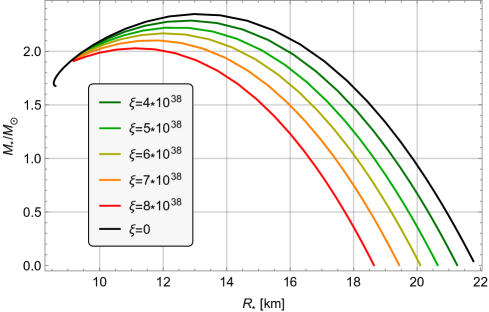
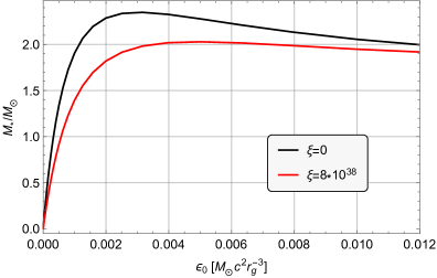
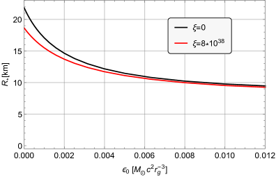
The mass-radius relation clearly depends on the scale at which the gravitational antiscreening becomes important. As already mentioned, this scale is parametrised by the positive constant $\xi$. The modified mass-radius relation is shown in Fig. 1 for different values of $\xi$. Unsurprisingly, a sizable effect on the mass and radius of a star requires to raise the scale of quantum gravity to macroscopic scales, by setting $\xi^{2}\gtrsim 10^{76}$. This enormous value for $\xi^{2}$ is due to the suppression factor $\epsilon_{\mathrm{Pl}}^{-1}$, Eq. (5.4), which enters the expression (5.3) for the effective energy density $\epsilon_{\rm q}$. As already noticed, the antiscreening effects induced by the running gravitational coupling (5.1) decrease the value of the effective mass $M_{\rm q}(R_{\ast})$, thus favouring the formation of lighter and smaller neutron stars. This is explicitly shown in Fig. 2, where the classical (black line, $\xi=0$) and quantum-modified (red line, $\xi=8\cdot 10^{38}$) mass and radius are shown as functions of the central density $\epsilon_{0}$.

   

Figure 2: Dependence of mass $M_{*}$ (left panel) and radius $R_{*}$ (right panel) on the central density $\epsilon_{0}$. The black line ($\xi=0$) reproduces the classical case, whereas the red line is obtained in the quantum-modified case for $\xi=8\cdot 10^{38}$.

6 Quantum-corrected Buchdahl limit

In this section we study the TOV equation for an incompressible fluid characterized by a constant energy density $\epsilon=\epsilon_{0}$. Although the energy density in a realistic star interior certainly depends on the radial coordinate $r$, assuming $\epsilon=\epsilon_{0}$ has the advantage of not requiring an EoS as an input to solve the TOV equation and allows to derive an important theoretical bound, known as the Buchdahl limit, for stars with isotropic pressure [82]. In General Relativity, the latter is parametrized by a curve in the $(M_{\ast}-R_{\ast})$-plane corresponding to spherically symmetric self-gravitating objects with diverging central pressure. In what follows we will discuss how this classical limit is modified by antiscreening effects of gravity.

We start by reviewing the derivation of the Buchdahl limit in the classical case. The mass of the star is obtained by integrating Eq. (2.8) for a constant energy density $\epsilon_{0}=\rho_{0}\,c^{2}$,

$$M(r)=\frac{4\,\pi\,r^{3}}{3}\,\rho_{0}=\frac{M_{*}\,r^{3}}{R_{*}^{3}}\ ,$$ (6.1)

where we used

$$\rho_{0}=\frac{3\,M_{\ast}}{4\,\pi\,R_{\ast}^{3}}$$ (6.2)

for the total mass density. The isotropic hydrostatic pressure $p=p(r)$ is then derived by replacing Eq. (6.1) into the classical TOV equation (2.9), and solving with the boundary condition $p(R_{\ast})=0$. The central pressure reads

$$p(0)=-\frac{3\,c^{2}\,M_{*}\left[3\,G_{0}\,M_{\ast}+c^{2}\,R_{\ast}\,\left(\sqrt{1-\frac{2\,G_{0}\,M_{\ast}}{R_{\ast}\,c^{2}}}-1\right)\right]}{4\,\pi\,R_{\ast}^{3}\,(4\,c^{2}\,R_{\ast}-9\,G_{0}\,M_{\ast})}\ .$$ (6.3)

The condition $p^{-1}(r=0)>0$, ensuring a finite and positive central pressure , thus imposes the Buchdahl bound

$$M_{\ast}<\frac{4\,c^{2}}{9\,G_{0}}\,R_{\ast}\ .$$ (6.4)

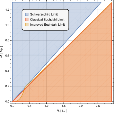
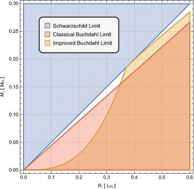
The allowed region in the $(M_{\ast}-R_{\ast})$-plane is shown in the left panel of Fig. 3 (orange region), together with the region $R_{\ast}>2\,M_{\ast}\,G_{0}/c^{2}$ corresponding to astrophysical objects whose radius is inside the Schwarzschild radius (blue region).

   

Figure 3: Graphical representation of the Buchdahl limit in the classical (orange region) and quantum-improved case (yellow region), for $\xi=g_{\ast}=1$, in Planck units. Astrophysical objects with radius $R_{\ast}<2\,M_{\ast}G_{0}/c^{2}$ fall into the blue region, delimited by the classical Schwarzschild limit. The white region in between is a transient region and accommodates astrophysical objects characterized by a negative central pressure. For large masses and radii the classical and modified Buchdahl limits coincide, whereas modifications due to the running of the gravitational coupling occur at Planckian scales (see left panel). In particular, there exists a critical radius $R_{\ast}\simeq 0.37\,L_{\rm Pl}$, where the improved Buchdahl-limit curve meets the classical Schwarzschild limit, $R_{\ast}=2\,M_{\ast}\,G_{0}/c^{2}$. Below this critical point, i.e., for $R\lesssim R_{\ast}^{\mathrm{crit}}$, the internal structure of stars changes so that the Buchdahl limit is met when $M_{\ast}\sim(R_{\ast}/L_{\mathrm{Pl}})^{3}M_{\mathrm{Pl}}$, according to Eq. (6.12). A magnified view of the sub-Planckian region including the critical point is shown in the right panel.

Modifications induced by the energy dependence of the gravitational coupling can now be obtained by following the same steps. We first need to solve Eq. (4.3) for a constant energy density $\epsilon_{0}=\rho_{0}\,c^{2}$. The corresponding mass function is given by

$$M_{\rm q}(r)=\frac{4\,\pi\,r^{3}}{3}\left[\frac{{\log}\left(1+\xi^{2}\,g_{\ast}^{-1}\epsilon_{\mathrm{Pl}}^{-1}\,\rho_{0}\,c^{2}\right)}{\xi^{2}\,g_{\ast}^{-1}\,\epsilon_{\mathrm{Pl}}^{-1}\,c^{2}}\right]\ ,$$ (6.5)

so that a star of radius $R_{\ast}$ and mass $M_{\ast}=M_{\rm q}(R_{\ast})$ has an effective mass density

$$\rho_{0}=\left[\exp\left(\frac{\xi^{2}c^{2}}{g_{\ast}\,\epsilon_{\mathrm{Pl}}}\,\frac{3\,M_{\ast}}{4\,\pi\,R_{\ast}^{3}}\right)-1\right]\frac{g_{\ast}\,\epsilon_{\mathrm{Pl}}}{\xi^{2}c^{2}}\ .$$ (6.6)

Note that, for objects of small compactness, $G_{0}\,M_{*}\ll c^{2}\,R_{*}$, the above expressions just reproduce their general relativistic analogues, Eq. (6.1) and (6.2). Employing Eqs. (6.6) and (6.5), the new TOV equation (4.9) can be integrated to give an explicit expression for the pressure of the star. In the center, it is given by

$$p(0)=\frac{\epsilon_{\mathrm{Pl}}}{\xi^{2}g_{\ast}^{-1}}\,\frac{\mathcal{N}(R_{\ast},M_{\ast})}{\mathcal{D}(R_{\ast},M_{\ast})}\ ,$$ (6.7)

with

$$\mathcal{N}= \left(e^{\frac{\xi^{2}c^{2}}{g_{\ast}\epsilon_{\mathrm{Pl}}}\,\frac{3\,M_{\ast}}{4\,\pi\,R_{\ast}^{3}}}-1\right)\left[\xi^{2}g_{\ast}^{-1}M_{\ast}\,e^{\frac{\xi^{2}c^{2}}{g_{\ast}\,\epsilon_{\mathrm{Pl}}}\frac{3\,M_{\ast}}{4\,\pi\,R_{\ast}^{3}}}-2\,\pi\,R_{\ast}^{3}\,\frac{\epsilon_{\mathrm{Pl}}}{c^{2}}\left(e^{\frac{\xi^{2}c^{2}}{g_{\ast}\,\epsilon_{\mathrm{Pl}}}\,\frac{3\,M_{\ast}}{4\,\pi\,R_{\ast}^{3}}}-1\right)\right]$$

$$\times\left(\sqrt{1-\frac{2\,G_{0}\,M_{\ast}}{R_{\ast}\,c^{2}}}-1\right)$$ (6.8)

and

$$\mathcal{D}=\xi^{2}g_{\ast}^{-1}\,M_{\ast}\,e^{\frac{\xi^{2}c^{2}}{g_{\ast}\,\epsilon_{\mathrm{Pl}}}\,\frac{3\,M_{\ast}}{4\,\pi\,R_{\ast}^{3}}}+2\,\pi\,R_{\ast}^{3}\,\frac{\epsilon_{\mathrm{Pl}}}{c^{2}}\left(e^{\frac{\xi^{2}c^{2}}{g_{\ast}\,\epsilon_{\mathrm{Pl}}}\,\frac{3\,M_{\ast}}{4\,\pi\,R_{\ast}^{3}}}-1\right)\left(\sqrt{1-\frac{2\,G_{0}\,M_{\ast}}{R_{\ast}\,c^{2}}}-1\right).$$ (6.9)

The condition $p^{-1}(r=0)>0$ defines the quantum-improved Buchdahl bound (yellow region in Fig. 3). For large masses and radii, the limiting curve $p^{-1}(r=0)=0$ coincides with the classical Buchdahl limit (6.4). Zooming into the Planckian region, where ultra-compact stars of Planckian masses are located, this limiting curve starts deviating from the classical one (see left panel of Fig. 3), and gets closer to the Schwarzschild limit. Our modified TOV equation thus allows for the existence of ultra-compact horizonless objects of positive central pressure beyond the classical Buchdahl limit. The radius of these Planckian stars is very close to the Schwarzschild radius. As a consequence, similarly to the “quasi-black-holes” introduced in Refs. [83, 84], these ultra-compact objects would appear dark to distant observers.

Interestingly, there exists a critical point $(R_{\ast}^{\mathrm{crit}},M_{\ast}^{\mathrm{crit}})$ where the modified Buchdahl bound matches the Schwartzschild limit. The value of the critical radius $R_{\ast}^{\mathrm{crit}}$ can be derived analytically from the condition $\mathcal{D}(R_{\ast},R_{\ast}c^{2}/2G_{0})=0$ and reads

$$R_{\ast}^{\rm crit}=L_{\mathrm{Pl}}\,\sqrt{\frac{\xi^{2}\,g_{\ast}^{-1}}{4\,\pi\left[1+\frac{2}{3}\mathcal{W}\left(-\frac{3}{2}\,e^{-3/2}\right)\right]}}\simeq 0.37\,\sqrt{\xi^{2}\,g_{\ast}^{-1}}\,L_{\mathrm{Pl}}\ ,$$ (6.10)

where $L_{\mathrm{Pl}}$ is the Planck length and $\mathcal{W}$ is the Lambert W-function. The existence of a critical value is due to the presence of the non-trivial fixed point $g_{\ast}$, reminiscent of the non-perturbative renormalizability of gravity. Naturally, in the classical limit $g_{\ast}\to\infty$ (or, equivalently, $\xi\to 0$) and the critical radius $R_{\ast}^{\rm crit}$ vanishes.

Beyond the critical point, the Buchdahl limit undergoes a major deviation from the classical case, indicating a possible transition to a new phase, dominated by quantum-gravitational fluctuations. In fact, crossing the critical point, the function $\mathcal{D}(R_{\ast},M_{\ast})$ becomes negative and the Buchdahl condition reduces to the inequality $\mathcal{N}(R_{\ast},M_{\ast})<0$. The latter can be solved exactly and gives a quantum-improved Buchdahl limit for sub-Planckian stars,

$$M_{\ast}<\frac{2\,\pi\,c^{5}\left[1+\frac{2}{3}\,\mathcal{W}\left(-\frac{3}{2}\,e^{-3/2}\right)\right]}{\hbar\,\xi^{2}g_{\ast}^{-1}\,G_{0}^{2}}\,R_{\ast}^{3}\ .$$ (6.11)

The above equation is equivalent to the condition

$$R_{\ast}\gtrsim\,0.27\,\xi^{2}g_{\ast}^{-1}\left(\frac{M_{\ast}}{M_{\mathrm{Pl}}}\right)^{\frac{1}{3}}L_{\mathrm{Pl}}$$ (6.12)

and, interestingly, the critical line $R_{\ast}\sim(M_{\ast}/M_{\mathrm{Pl}})^{1/3}\,L_{\mathrm{Pl}}$ resembles the scaling relation characterizing “Planck stars” of the kind introduced in Ref. [95]. As is clear from Eq. (6.11), below the critical point the quantum-corrected Buchdahl limit deviates substantially from the classical one. This transition occurs in the sub-Planckian region, as shown in the right panel of Fig. 3. At variance with the case $R_{\ast}^{\mathrm{crit}}<R_{\ast}\lesssim L_{\mathrm{Pl}}$, below the critical point the formation of stars of positive central pressure is more restricted. However, the new bound (6.12) still allows for the existence of astrophysical objects with arbitrarily small radii.

7 Conclusions

The approach discussed in this paper allows the study of stellar structure equilibrium configurations in theories with energy-dependent gravitational interaction. This dependence could arise, e.g., from the running of the gravitational couplings dictated by the renormalization group equations.

Unless the scale of quantum gravity is much below the Planck scale, quantum-gravity effects cannot affect the mass-radius relation of standard neutron stars. However, our formalism is useful to describe possible outcomes of the gravitational collapse when the internal density reaches Planckian values. In particular the new, quantum-improved, stellar structure equations could be used to discuss possible non-singular stellar-like remnants. Clearly, in order to address the latter point, it is essential to study the stability of these new configurations. Classical secular stability can be discussed in terms of the critical points of the mass $M_{\ast}(\rho_{0})$, where $\rho_{0}$ is the central mass density. In our case, unless the running of Newton coupling is negligible, this criterion cannot be used. It is thereby essential to study the spectrum of the stability equations for the radial modes induced by the effective energy-momentum tensor (3.5). We defer this point to a following paper.

Assuming that the running of the Newton coupling is given by Eq. (5.1) and a polytropic equation of state (our arguments can be easily generalized to the case of piecewise equation of states), the most important result of our investigation is the possible existence of ultra-compact objects of Planckian size, as is displayed in Fig. 3. These Planckian stars would be completely dark for any astrophysical purpose, yet they would have no horizon. They could have been produced by direct collapse of primordial perturbations during the inflationary era and subsequently merged to produce primordial black holes [96, 97, 98, 99]. It would thus be interesting to study the phenomenological consequences of our findings.

Appendix A Varying the matter Lagrangian

In this Appendix, we derive the variation (3.3) for the proper energy density following closely Ref. [100]. Our convention for the metric signature is $(+---)$.

Let us consider a generic fluid of baryonic density $\rho$. The baryonic density is a density function satisfying the continuity equation for vanishing pressure

$$\nabla_{\mu}\left(\rho\,u^{\mu}\right)=\frac{1}{\sqrt{-g}}\,\partial_{\mu}\left(\sqrt{-g}\,\rho\,u^{\mu}\right)=0\ ,$$ (A.1)

where $u^{\mu}$ is the fluid’s 4-velocity in a general reference frame $x^{\mu}$. Specifically, $u^{\mu}=\frac{\mbox{${\rm d}$}x^{\mu}}{\mbox{${\rm d}$}\tau_{x}}$, with the proper time implicitly defined by

$$c^{2}\mbox{${\rm d}$}\tau_{x}^{2}=g_{\mu\nu}(x^{\sigma})\,\mbox{${\rm d}$}x^{\mu}\,\mbox{${\rm d}$}x^{\nu}\ .$$ (A.2)

The relation (A.1) depends on the metric, both explicitly via the determinant $g$ and implicitly in the definition (A.2) of proper time $\tau_{x}$. However, $\rho$ is a scalar under change of coordinates, so that the same continuity equation must also hold in the frame $X^{\alpha}=X^{\alpha}(x^{\mu})$ comoving with the fluid. In this frame, the fluid’s proper time along a trajectory $X^{\alpha}=X^{\alpha}(\tau_{X})$ is given by

$$c^{2}\mbox{${\rm d}$}\tau_{X}^{2}=G_{00}(X^{\alpha})\,\mbox{${\rm d}$}X^{0}\,\mbox{${\rm d}$}X^{0}=g_{\mu\nu}(x^{\sigma})\,\frac{\partial x^{\mu}}{\partial X^{0}}\,\frac{\partial x^{\nu}}{\partial X^{0}}\,\mbox{${\rm d}$}X^{0}\,\mbox{${\rm d}$}X^{0}\ ,$$ (A.3)

and the 4-velocity is

$$U^{\alpha}=\frac{\mbox{${\rm d}$}X^{\alpha}}{\mbox{${\rm d}$}\tau_{X}}=\frac{\delta^{\alpha}_{0}}{c^{-1}\left[g_{\mu\nu}\,\frac{\partial x^{\mu}}{\partial X^{0}}\,\frac{\partial x^{\nu}}{\partial X^{0}}\right]^{1/2}}\ .$$ (A.4)

The continuity equation in the comoving frame reads

$$\frac{1}{\sqrt{-G}}\,\partial_{0}\left(\sqrt{-G}\,\rho\,U^{0}\right)=0\ ,$$ (A.5)

and can be integrated to yield

$$\sqrt{-g}\,\left|\frac{\partial x}{\partial X}\right|\,\rho=\sqrt{-G}\,\rho=K\,\left[g_{\mu\nu}\,\frac{\partial x^{\mu}}{\partial X^{0}}\,\frac{\partial x^{\nu}}{\partial X^{0}}\right]^{1/2}\ ,$$ (A.6)

where $K$ is an integration constant and $\left|\frac{\partial x}{\partial X}\right|$ the modulus of the Jacobian of the transformation $x^{\mu}=x^{\mu}(X^{\alpha})$, which does not depend on the metric. It follows that

$$\delta\left(\sqrt{-g}\,\left|\frac{\partial x}{\partial X}\right|\,\rho\right)=\left|\frac{\partial x}{\partial X}\right|\delta\left(\sqrt{-g}\,\,\rho\right)=\frac{K}{2}\left[g_{\mu\nu}\,\frac{\partial x^{\mu}}{\partial X^{0}}\,\frac{\partial x^{\nu}}{\partial X^{0}}\right]^{-1/2}\frac{\partial x^{\sigma}}{\partial X^{0}}\,\frac{\partial x^{\lambda}}{\partial X^{0}}\,\delta g_{\sigma\lambda}$$ (A.7)

At this point, we just need to use Eq. (A.6) and note that

$$u^{\sigma}=\frac{\partial x^{\sigma}}{\partial X^{0}}\,U^{0}=c\,\frac{\partial x^{\sigma}}{\partial X^{0}}\left[g_{\mu\nu}\,\frac{\partial x^{\mu}}{\partial X^{0}}\,\frac{\partial x^{\nu}}{\partial X^{0}}\right]^{-1/2}\ ,$$ (A.8)

in order to finally obtain

$$\delta\left(\sqrt{-g}\,\rho\right)=\frac{1}{2}\,\sqrt{-g}\left(\rho\,c^{-2}u^{\mu}\,u^{\nu}\right)\delta g_{\mu\nu}=-\frac{1}{2}\,\sqrt{-g}\left(\rho\,c^{-2}u_{\mu}\,u_{\nu}\right)\delta g^{\mu\nu}\ .$$ (A.9)

Expanding the variation in the left-hand-side of this expression and using the well-known relation for the variation of the metric determinant, we obtain

$$\delta\rho=\frac{\rho}{2}\left(g_{\mu\nu}-c^{-2}u_{\mu}\,u_{\nu}\right)\delta g^{\mu\nu}\ .$$ (A.10)

For a barotropic perfect fluid, the pressure is a function of the proper energy density only, $p=p(\epsilon)$. In this case the baryonic density $\rho$ and the proper energy density $\epsilon$ are related to each other by means of the following relation [101]

$$\frac{\delta\rho}{\rho}=\frac{\delta\epsilon}{\epsilon+p(\epsilon)}\ .$$ (A.11)

Combining this relation with Eq. (A.10), finally yields the variation (3.3) of the proper energy density relevant for the derivation of the field equations in the Markov-Mukhanov formalism reported in Sect. 3.

References

- [1] Daniele Malafarina. Classical collapse to black holes and quantum bounces: A review. Universe, 3(2):48, 2017.
- [2] S. Weinberg. Ultraviolet divergences in quantum theories of gravitation. In S. W. Hawking and W. Israel, editors, General Relativity: An Einstein centenary survey, pages 790–831, 1979.
- [3] C. Wetterich. Exact evolution equation for the effective potential. Physics Letters B, 301:90–94, February 1993.
- [4] M. Reuter. Nonperturbative evolution equation for quantum gravity. Phys. Rev., D57:971–985, 1998.
- [5] W. Souma. Non-Trivial Ultraviolet Fixed Point in Quantum Gravity. Progress of Theoretical Physics, 102:181–195, July 1999.
- [6] O. Lauscher and M. Reuter. Flow equation of quantum Einstein gravity in a higher-derivative truncation. Phys. Rev. D, 66(2):025026, July 2002.
- [7] A. Codello and R. Percacci. Fixed Points of Higher-Derivative Gravity. Physical Review Letters, 97(22):221301, December 2006.
- [8] P. F. Machado and F. Saueressig. On the renormalization group flow of f(R)-gravity. Phys. Rev. D, 77:124045, 2008.
- [9] D. Benedetti, P. F. Machado, and F. Saueressig. Asymptotic Safety in Higher-Derivative Gravity. Modern Physics Letters A, 24:2233–2241, 2009.
- [10] K. Falls and N. Ohta. Renormalization group equation for f(R) gravity on hyperbolic spaces. Phys. Rev. D, 94(8):084005, October 2016.
- [11] H. Gies, B. Knorr, S. Lippoldt, and F. Saueressig. Gravitational Two-Loop Counterterm Is Asymptotically Safe. Physical Review Letters, 116(21):211302, May 2016.
- [12] Yuta Hamada and Masatoshi Yamada. Asymptotic safety of higher derivative quantum gravity non-minimally coupled with a matter system. JHEP, 08:070, 2017.
- [13] Gustavo P. De Brito, Nobuyoshi Ohta, Antonio D. Pereira, Anderson A. Tomaz, and Masatoshi Yamada. Asymptotic safety and field parametrization dependence in the truncation. 2018.
- [14] P. Donà, A. Eichhorn, and R. Percacci. Matter matters in asymptotically safe quantum gravity. Phys. Rev. D, 89(8):084035, April 2014.
- [15] P. Donà, A. Eichhorn, and R. Percacci. Consistency of matter models with asymptotically safe quantum gravity. Canadian Journal of Physics, 93:988–994, September 2015.
- [16] J. Meibohm, J. M. Pawlowski, and M. Reichert. Asymptotic safety of gravity-matter systems. Phys. Rev. D, 93(8):084035, April 2016.
- [17] K. Y. Oda and M. Yamada. Non-minimal coupling in Higgs-Yukawa model with asymptotically safe gravity. Classical and Quantum Gravity, 33(12):125011, June 2016.
- [18] P. Donà, A. Eichhorn, P. Labus, and R. Percacci. Asymptotic safety in an interacting system of gravity and scalar matter. Phys. Rev. D, 93(4):044049, February 2016.
- [19] A. Eichhorn, A. Held, and J. M. Pawlowski. Quantum-gravity effects on a Higgs-Yukawa model. Phys. Rev. D, 94(10):104027, November 2016.
- [20] Nicolai Christiansen, Daniel F. Litim, Jan M. Pawlowski, and Manuel Reichert. Asymptotic safety of gravity with matter. Phys. Rev., D97(10):106012, 2018.
- [21] Astrid Eichhorn, Stefan Lippoldt, and Marc Schiffer. Zooming in on fermions and quantum gravity. Phys. Rev., D99(8):086002, 2019.
- [22] Astrid Eichhorn and Marc Schiffer. as the critical dimensionality of asymptotically safe interactions. Phys. Lett., B793:383–389, 2019.
- [23] Astrid Eichhorn. On unimodular quantum gravity. Class. Quant. Grav., 30:115016, 2013.
- [24] Dario Benedetti. Essential nature of Newton’s constant in unimodular gravity. Gen. Rel. Grav., 48(5):68, 2016.
- [25] Astrid Eichhorn. The Renormalization Group flow of unimodular f(R) gravity. JHEP, 04:096, 2015.
- [26] Gustavo P. De Brito, Astrid Eichhorn, and Antonio D. Pereira. A link that matters: Towards phenomenological tests of unimodular asymptotic safety. JHEP, 09:100, 2019.
- [27] E. Manrique, S. Rechenberger, and F. Saueressig. Asymptotically Safe Lorentzian Gravity. Physical Review Letters, 106(25):251302, June 2011.
- [28] Jorn Biemans, Alessia Platania, and Frank Saueressig. Quantum gravity on foliated spacetimes: Asymptotically safe and sound. Phys. Rev., D95(8):086013, 2017.
- [29] Jorn Biemans, Alessia Platania, and Frank Saueressig. Renormalization group fixed points of foliated gravity-matter systems. JHEP, 05:093, 2017.
- [30] W. B. Houthoff, A. Kurov, and F. Saueressig. Impact of topology in foliated Quantum Einstein Gravity. Eur. Phys. J., C77:491, 2017.
- [31] Alessia Platania and Frank Saueressig. Functional Renormalization Group Flows on Friedman–Lemaître–Robertson–Walker backgrounds. Found. Phys., 48(10):1291–1304, 2018.
- [32] Benjamin Knorr. Lorentz symmetry is relevant. Phys. Lett., B792:142–148, 2019.
- [33] Kevin Falls, Callum R. King, Daniel F. Litim, Kostas Nikolakopoulos, and Christoph Rahmede. Asymptotic safety of quantum gravity beyond Ricci scalars. Phys. Rev., D97(8):086006, 2018.
- [34] Kevin G. Falls, Daniel F. Litim, and Jan Schröder. Aspects of asymptotic safety for quantum gravity. Phys. Rev., D99(12):126015, 2019.
- [35] F. Fayos and R. Torres. A quantum improvement to the gravitational collapse of radiating stars. Classical and Quantum Gravity, 28(10):105004, May 2011.
- [36] Alfio Bonanno and Martin Reuter. Renormalization group improved black hole space-times. Phys. Rev., D62:043008, 2000.
- [37] A. Bonanno and M. Reuter. Spacetime structure of an evaporating black hole in quantum gravity. Phys. Rev., D73:083005, 2006.
- [38] Kevin Falls and Daniel F. Litim. Black hole thermodynamics under the microscope. Phys. Rev., D89:084002, 2014.
- [39] Benjamin Koch and Frank Saueressig. Structural aspects of asymptotically safe black holes. Class. Quant. Grav., 31:015006, 2014.
- [40] Georgios Kofinas and Vasilios Zarikas. Avoidance of singularities in asymptotically safe Quantum Einstein Gravity. JCAP, 1510(10):069, 2015.
- [41] Alfio Bonanno, Benjamin Koch, and Alessia Platania. Cosmic Censorship in Quantum Einstein Gravity. Class. Quant. Grav., 34(9):095012, 2017.
- [42] Alfio Bonanno, Benjamin Koch, and Alessia Platania. Asymptotically Safe gravitational collapse: Kuroda-Papapetrou RG-improved model. PoS, corfu2016:058, 2017.
- [43] Alfio Bonanno, Benjamin Koch, and Alessia Platania. Gravitational collapse in Quantum Einstein Gravity. 2017.
- [44] Ramon Torres. Nonsingular black holes, the cosmological constant, and asymptotic safety. Phys. Rev., D95(12):124004, 2017.
- [45] Jan M. Pawlowski and Dennis Stock. Quantum-improved Schwarzschild-(A)dS and Kerr-(A)dS spacetimes. Phys. Rev., D98(10):106008, 2018.
- [46] Ademola Adeifeoba, Astrid Eichhorn, and Alessia Platania. Towards conditions for black-hole singularity-resolution in asymptotically safe quantum gravity. Class. Quant. Grav., 35(22):225007, 2018.
- [47] Aaron Held, Roman Gold, and Astrid Eichhorn. Asymptotic safety casts its shadow. JCAP, 1906(06):029, 2019.
- [48] Alessia Platania. Dynamical renormalization of black-hole spacetimes. Eur. Phys. J., C79(6):470, 2019.
- [49] A. Bonanno and M. Reuter. Cosmology with self-adjusting vacuum energy density from a renormalization group fixed point. Physics Letters B, 527:9–17, February 2002.
- [50] A. Bonanno and M. Reuter. Cosmology of the Planck era from a renormalization group for quantum gravity. Phys. Rev. D, 65(4):043508, February 2002.
- [51] B. Guberina, R. Horvat, and H. Štefančić. Renormalization-group running of the cosmological constant and the fate of the universe. Phys. Rev. D, 67(8):083001, April 2003.
- [52] M. Reuter and Frank Saueressig. From big bang to asymptotic de Sitter: Complete cosmologies in a quantum gravity framework. JCAP, 0509:012, 2005.
- [53] A. Bonanno and M. Reuter. Entropy signature of the running cosmological constant. JCAP, 8:024, August 2007.
- [54] S. Weinberg. Asymptotically safe inflation. Phys. Rev. D, 81(8):083535, April 2010.
- [55] A. Bonanno. An effective action for asymptotically safe gravity. Phys. Rev. D, 85(8):081503, April 2012.
- [56] M. Hindmarsh and I. D. Saltas. f(R) gravity from the renormalization group. Phys. Rev. D, 86(6):064029, September 2012.
- [57] Edmund J. Copeland, Christoph Rahmede, and Ippocratis D. Saltas. Asymptotically Safe Starobinsky Inflation. Phys. Rev., D91(10):103530, 2015.
- [58] Georgios Kofinas and Vasilios Zarikas. Asymptotically Safe gravity and non-singular inflationary Big Bang with vacuum birth. Phys. Rev., D94(10):103514, 2016.
- [59] Alfio Bonanno and Alessia Platania. Asymptotically safe inflation from quadratic gravity. Phys. Lett., B750:638–642, 2015.
- [60] Alfio Bonanno and Alessia Platania. Asymptotically Safe R+R2 gravity. PoS, corfu2015:159, 2016.
- [61] Alfio Bonanno, S. J. Gabriele Gionti, and Alessia Platania. Bouncing and emergent cosmologies from Arnowitt-Deser-Misner RG flows. Class. Quant. Grav., 35(6):065004, 2018.
- [62] Alfio Bonanno, Alessia Platania, and Frank Saueressig. Cosmological bounds on the field content of asymptotically safe gravity-matter models. 2018.
- [63] Alessia Platania. The inflationary mechanism in Asymptotically Safe Gravity. Universe, 5(8):189, 2019.
- [64] Alfio Bonanno and Frank Saueressig. Asymptotically safe cosmology – A status report. Comptes Rendus Physique, 18:254–264, 2017.
- [65] G. K. Savvidy. Infrared Instability of the Vacuum State of Gauge Theories and Asymptotic Freedom. Phys. Lett., 71B:133–134, 1977.
- [66] A. Nink and M. Reuter. On the physical mechanism underlying asymptotic safety. Journal of High Energy Physics, 1:62, January 2013.
- [67] M. A. Markov and V. F. Mukhanov. De Sitter-like initial state of the universe as a result of asymptotical disappearance of gravitational interactions of matter. Nuovo Cimento B Serie, 86:97–102, 1985.
- [68] Richard C. Tolman. Static solutions of Einstein’s field equations for spheres of fluid. Phys. Rev., 55:364–373, 1939.
- [69] J. R. Oppenheimer and G. M. Volkoff. On Massive neutron cores. Phys. Rev., 55:374–381, 1939.
- [70] Hans Stephani. Relativity: An introduction to special and general relativity. 2004.
- [71] A. D. Sakharov. Vacuum quantum fluctuations in curved space and the theory of gravitation. Sov. Phys. Dokl., 12:1040–1041, 1968. [,51(1967)].
- [72] T. Padmanabhan. Emergent Gravity Paradigm: Recent Progress. Mod. Phys. Lett., A30(03n04):1540007, 2015.
- [73] Erik P. Verlinde. Emergent Gravity and the Dark Universe. SciPost Phys., 2(3):016, 2017.
- [74] Gia Dvali and Cesar Gomez. Quantum Compositeness of Gravity: Black Holes, AdS and Inflation. JCAP, 1401:023, 2014.
- [75] Andrea Giusti. On the corpuscular theory of gravity. Int. J. Geom. Meth. Mod. Phys., 16(03):1930001, 2019.
- [76] Mariano Cadoni, Roberto Casadio, Andrea Giusti, Wolfgang Mueck, and Matteo Tuveri. Effective Fluid Description of the Dark Universe. Phys. Lett., B776:242–248, 2018.
- [77] M. Cadoni, R. Casadio, A. Giusti, and M. Tuveri. Emergence of a Dark Force in Corpuscular Gravity. Phys. Rev., D97(4):044047, 2018.
- [78] Roberto Casadio, Andrea Giugno, and Andrea Giusti. Corpuscular slow-roll inflation. Phys. Rev., D97(2):024041, 2018.
- [79] Roberto Casadio, Michele Lenzi, and Octavian Micu. Bootstrapped Newtonian stars and black holes. 2019.
- [80] Roberto Casadio, Michele Lenzi, and Octavian Micu. Bootstrapping Newtonian gravity. Phys. Rev., D98(10):104016, 2018.
- [81] Raul Carballo-Rubio. Stellar equilibrium in semiclassical gravity. Phys. Rev. Lett., 120(6):061102, 2018.
- [82] Hans A. Buchdahl. General Relativistic Fluid Spheres. Phys. Rev., 116:1027, 1959.
- [83] Jose P. S. Lemos and Oleg B. Zaslavskii. Quasi black holes: Definition and general properties. Phys. Rev., D76:084030, 2007.
- [84] Carlos Barcelo, Stefano Liberati, Sebastiano Sonego, and Matt Visser. Fate of gravitational collapse in semiclassical gravity. Phys. Rev., D77:044032, 2008.
- [85] R. Arnowitt, S. Deser, and C. W. Misner. Dynamical Structure and Definition of Energy in General Relativity. Physical Review, 116:1322–1330, December 1959.
- [86] M. Niedermaier and M. Reuter. The Asymptotic Safety Scenario in Quantum Gravity. Living Reviews in Relativity, 9:5, December 2006.
- [87] Olivier Minazzoli and Tiberiu Harko. New derivation of the Lagrangian of a perfect fluid with a barotropic equation of state. Phys. Rev., D86:087502, 2012.
- [88] Feryal Ozel, Dimitrios Psaltis, Ramesh Narayan, and Antonio Santos Villarreal. On the Mass Distribution and Birth Masses of Neutron Stars. Astrophys. J., 757:55, 2012.
- [89] N. Chamel, P. Haensel, J. L. Zdunik, and A. F. Fantina. On the Maximum Mass of Neutron Stars. Int. J. Mod. Phys., E22:1330018, 2013.
- [90] Ben Margalit and Brian D. Metzger. Constraining the Maximum Mass of Neutron Stars From Multi-Messenger Observations of GW170817. Astrophys. J., 850(2):L19, 2017.
- [91] H. Thankful Cromartie et al. Relativistic Shapiro delay measurements of an extremely massive millisecond pulsar. 2019.
- [92] Alfio Bonanno and Martin Reuter. Quantum gravity effects near the null black hole singularity. Phys. Rev., D60:084011, 1999.
- [93] Richard R. Silbar and Sanjay Reddy. Neutron stars for undergraduates. Am. J. Phys., 72:892–905, 2004. [Erratum: Am. J. Phys.73,286(2005)].
- [94] Camilo Posada and Cecilia Chirenti. On the radial stability of ultra compact Schwarzschild stars beyond the Buchdahl limit. Class. Quant. Grav., 36:065004, 2019.
- [95] Carlo Rovelli and Francesca Vidotto. Planck stars. Int. J. Mod. Phys., D23(12):1442026, 2014.
- [96] Bernard J. Carr and S. W. Hawking. Black holes in the early Universe. Mon. Not. Roy. Astron. Soc., 168:399–415, 1974.
- [97] Bernard J. Carr. The Primordial black hole mass spectrum. Astrophys. J., 201:1–19, 1975.
- [98] Bernard Carr, Florian Kuhnel, and Marit Sandstad. Primordial Black Holes as Dark Matter. Phys. Rev., D94(8):083504, 2016.
- [99] R. Casadio, A. Giugno, A. Giusti, and M. Lenzi. Quantum Formation of Primordial Black holes. Gen. Rel. Grav., 51(8):103, 2019.
- [100] T. Harko. The matter Lagrangian and the energy-momentum tensor in modified gravity with non-minimal coupling between matter and geometry. Phys. Rev., D81:044021, 2010.
- [101] P. H. Chavanis. Cosmology with a stiff matter era. Phys. Rev., D92(10):103004, 2015.