Windowed least-squares model reduction for dynamical systems

Abstract

This work proposes a windowed least-squares (WLS) approach for model-reduction of dynamical systems. The proposed approach sequentially minimizes the time-continuous full-order-model residual within a low-dimensional space–time trial subspace over time windows. The approach comprises a generalization of existing model reduction approaches, as particular instances of the methodology recover Galerkin, least-squares Petrov–Galerkin (LSPG), and space–time LSPG projection. In addition, the approach addresses key deficiencies in existing model-reduction techniques, e.g., the dependence of LSPG and space–time LSPG projection on the time discretization and the exponential growth in time exhibited by a posteriori error bounds for both Galerkin and LSPG projection. We consider two types of space–time trial subspaces within the proposed approach: one that reduces only the spatial dimension of the full-order model, and one that reduces both the spatial and temporal dimensions of the full-order model. For each type of trial subspace, we consider two different solution techniques: direct (i.e., discretize then optimize) and indirect (i.e., optimize then discretize). Numerical experiments conducted using trial subspaces characterized by spatial dimension reduction demonstrate that the WLS approach can yield more accurate solutions with lower space–time residuals than Galerkin and LSPG projection.

1 Introduction

Simulating parameterized dynamical systems arises in many applications across science and engineering. In many contexts, executing a dynamical-system simulation at a single parameter instance—which entails the numerical integration of a system of ordinary differential equations (ODEs)—incurs an extremely large computational cost. This occurs, for example, when the state-space dimension is large (e.g., due to fine spatial resolution when discretizing a partial differential equation) and/or when the number of time instances is large (e.g., due to time-step limitations incurred by stability or accuracy considerations). When the application is time critical or many query in nature, analysts must replace such large-scale parameterized dynamical-system models (which we refer to as the full-order model) with a low-cost approximation that makes the application tractable.

Projection-based reduced-order models (ROMs) comprise one such approximation strategy. First, these techniques execute a computationally expensive offline stage that computes a low-dimensional trial subspace on which the dynamical-system state can be well approximated (e.g., by computing state “snapshots” at different time and parameter instances, by solving Lyapunov equations). Second, these methods execute an inexpensive online stage during which they compute approximations to the dynamical-system trajectory that reside on this trial subspace via, e.g., projection of the full-order model or residual minimization.

Model reduction for linear-time-invariant systems (and other well structured dynamical systems) is quite mature [7, 46, 48, 33], as system-theoretic properties (e.g., controllability, observability, asymptotic stability, $\mathcal{H}_{2}$-optimality) can be readily quantified and accounted for; this often results in reduced-order models that inherit such important properties. The primary challenge in developing reduced-order models for general nonlinear dynamical systems is that such properties are difficult to assess quantitatively. As a result, it is challenging to develop reduced-order models that preserve important dynamical-system properties, which often results in methods that yield trajectories that are inaccurate, unstable, or violate physical properties. To address this, researchers have pursued several directions that aim to imbue reduced-order models for nonlinear dynamical systems with properties that can improve robustness and accuracy. These efforts include residual-minimization approaches that equip the ROM solution with a notion of optimality [19, 21, 41, 43, 42, 13, 14, 54, 16, 12, 1]; space–time approaches that lead to error bounds that grow slowly in time [25, 26, 62, 68, 5]; “energy-based” inner products that ensure non-increasing entropy in the ROM solution [55, 36, 23]; basis-adaptation methods that improve the ROM’s accuracy a posteriori [17, 51, 29], stabilizing subspace rotations that account for truncated modes a priori [2], structure-preserving methods that enforce conservation [20] or (port-)Hamiltonian/Lagrangian structure [39, 22, 6, 24, 31] in the ROM; and subgrid-scale modeling methods that aim to improve accuracy by addressing the closure problem [59, 58, 35, 8, 15, 66, 67, 65, 60]. We note that these techniques are often not mutually exclusive. Residual-minimizing and space–time approaches are the most relevant classes of methods for the current work and comprise the focus of the following review.

Residual-minimization methods in model reduction compute the solution within a low-dimensional trial subspace that minimizes the full-order-model residual. Researchers have developed such residual-minimizing model-reduction methods for both static systems (i.e., systems without time-dependence) [41, 43, 42, 13, 54, 16, 12] and dynamical systems [12, 14, 16, 21, 19, 18]. In the latter category, Refs. [12, 14, 16, 21, 19] formulated the residual minimization problem for dynamical systems by sequentially minimizing the time-discrete full-order-model residual (i.e., the residual arising after applying time discretization) at each time instance on the time-discretization grid. This formulation is often referred to as the least–squares Petrov–Galerkin (LSPG) method. Ref. [18] performed detailed analyses of this formulation and examined its connections with Galerkin projection. Critically, this work demonstrated that (1) under certain conditions, LSPG can be cast as a Petrov–Galerkin projection applied to the time-continuous full-order-model residual, and (2) LSPG and Galerkin projection are equivalent in the limit as the time step goes to zero (i.e., Galerkin projection minimizes the time-instantaneous full-order-model residual). Numerous numerical experiments have demonstrated that LSPG often yields more accurate and stable solutions than Galerkin [12, 18, 21, 16, 50]. The common intuitive explanation for this improved performance is that, by minimizing the full-order-model residual over a finite time window (rather than time instantaneously), LSPG computes solutions that are more accurate over a larger part of the trajectory as compared to Galerkin.

However, LSPG has several notable shortcomings. First, LSPG exhibits a complex dependence on the time discretization. In particular, changing the time step ($\Delta t$) modifies both the time window over which LSPG minimizes the residual as well as the time-discretization error of the full-order model on which LSPG is based. As LSPG and Galerkin projection are equivalent in the limit of $\Delta t\rightarrow 0$, the accuracy of LSPG approaches the (sometimes poor) accuracy of Galerkin as the time step shrinks. For too-large a time step the accuracy of LSPG also degrades. It is unclear if this is due to the time-discretization error associated with enlarging the time step, or rather if it is due to the size of the window the residual is being minimized over. As a consequence, LSPG often yields the smallest error for an intermediate value of the time step (see, e.g., Ref. [18, Figure 9]); there is no known way to compute this optimal time step a priori. Second, as the LSPG approach performs sequential residual minimization in time, its a posteriori error bounds grow exponentially in time [18], and it is not equipped with any notion of optimality over the entire time domain of interest. As a result, LSPG is not equipped with a priori guarantees of accuracy or stability, even for linear time-invariant systems [12].

Researchers have pursued the development of space–time residual-minimization approaches [25, 26, 62, 68] to address the issues incurred by sequential residual minimization in time. Existing space–time approaches differ from the classic LSPG and Galerkin approaches in (1) the definition of the space–time trial subspace and (2) the definition of the residual minimization problem. First, space–time approaches leverage a space–time trial basis that characterizes both the spatial and temporal dependence of the state, classic “spatial” model reduction approaches such as LSPG and Galerkin leverage only a spatial trial basis that characterizes the spatial dependence of the state. Second, space–time residual minimization approaches compute the entire space–time trajectory of the state (within the low-dimensional space–time trial subspace) that minimizes the full-order-model residual over the entire time domain; Galerkin and LSPG sequentially compute instances of the state that either minimize the full-order model instantaneously (Galerkin) or over a time step (LSPG). The result of these differences is that space–time approaches yield a system of algebraic equations defined over all space and time, whose solution comprises a vector of (space–time) generalized coordinates; on the other hand, spatial-projection-only approaches generally associate with systems of ODEs whose solutions comprise time-dependent vectors of (spatial) generalized coordinates.

Space–time residual minimization approaches minimize the FOM residual over all of space and time and, as a result, yield models that are equipped with a notion of space–time optimality and a priori error bounds that grow more slowly in time. Further, space–time approaches reduce both the spatial and temporal dimensions of the full-order model, and thus promise cost savings over spatial-projection-only approaches. However, space–time techniques also suffer from several limitations. First, the computational cost of solving the algebraic system arising from space–time approaches scales cubically with the number of space–time degrees of freedom; in contrast, the computational cost incurred by standard spatial-projection-based ROMs is linear in the number of temporal degrees of freedom, as the attendant solvers can leverage the lower-block triangular structure of the system arising from the sequential nature of time evolution. As a result, solving the algebraic systems arising from space–time projection is generally intractable without applying hyper-reduction in time [25, 26]. Second, space–time residual minimization precludes future state prediction, as these methods employ space–time basis vectors defined over the entire time domain of interest, which must have been included in the training simulations.

The objectives of this work are to overcome the shortcomings of existing residual-minimizing methods, and to provide a unifying framework from which existing methods can be assessed. In essence, the proposed windowed least-squares (WLS) approach sequentially minimizes the FOM residual over a sequence of arbitrarily defined time windows. The method is characterized by three notable aspects. First, the method minimizes the time-continuous residual (i.e., that associated with the full-order model ODE). By adopting a time-continuous viewpoint, the formulation decouples the underlying temporal discretization scheme from the residual-minimization problem, thus addressing a key deficiency of both LSPG and space–time LSPG. Critically, time-continuous residual minimization also exposes two different solution methods: a discretize-then-optimize (i.e., direct) method, and an optimize-then-discretize (i.e., indirect) method. Second, the method sequentially minimizes the residual over arbitrarily defined time windows rather than sequentially minimizing the residual over time steps (as in LSPG) or over the entire time domain (as in space–time residual-minimization methods). This equips the method with additionally flexibility that enables it to explore more fine-grained tradeoffs between computational cost and error. Finally, WLS is formulated for two kinds of space–time trial subspaces: one that associates with spatial dimension reduction (as employed by traditional spatial-projection-based methods), and one that associates with space–time dimension reduction (as employed by space–time methods). The above attributes allow the WLS approach to be viewed as a generalization of existing model-reduction methods, as Galerkin, LSPG, and space–time LSPG projection correspond to specific instances of the formulation. Figure 1 depicts how the proposed WLS method provides a unifying framework from which these existing approaches can be derived.

The WLS approach can be viewed as a hybrid space–time method and displays commonalities with several related efforts. First, Ref. [12] briefly formulated a space–time least-squares ROM and connected this formulation with optimal control; specifically it mentioned the optimize-then-discretize vs. discretize-then-optimize approaches. This work did not fully develop this approach, eschewing it for sequential residual minimization in time (i.e., LSPG). The present work thus formally develops and extends several of the concepts put forth in Ref. [12]. Next, Ref. [26] developed a space–time residual minimization formulation for model interpolation. The present work distinguishes itself from Ref. [26] in that (1) this work also considers trial subspaces characterized by spatial dimension reduction only, and (2) we minimize the time-continuous FOM residual over arbitrary time windows. We note that, similar to the current work, Ref. [26] employs minimization of the time-continuous FOM residual as a starting point; as such, this work shares some thematic similarities with Ref. [26]. Lastly, Ref. [25] develops a space–time extension of LSPG projection that minimizes the time-discrete FOM residual over the entire time domain. The present work distinguishes itself from Ref. [25] in that (1) this work minimizes the time-continuous FOM residual, (2) this work minimizes this residual over arbitrary time windows, and (3) this work also considers trial subspaces associated with spatial dimension reduction only.

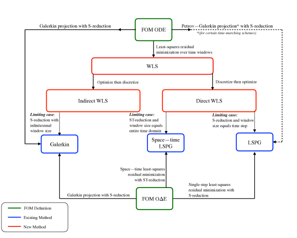
Figure 1: Relationship diagram for the WLS approach for model reduction.

In summary, specific contributions of this work include:

1. The windowed least-squares (WLS) approach for dynamical-system model reduction. The approach sequentially minimizes the time-continuous full-order-model residual over arbitrary time windows.

2. Support of two space–time trial subspaces: one that associates with spatial dimension reduction and one that associates with spatial and temporal dimension reduction. The former case is of particular interest in the WLS  context, as the stationary conditions are derived via the Euler–Lagrange equations and comprise a coupled two-point Hamiltonian boundary value problem containing a forward and backward system. The forward system, which is forced by an auxiliary costate, evolves the (spatial) generalized coordinates of the ROM in time. The backward system, which is forced by the time-continuous FOM residual evaluated about the ROM state, governs the dynamics of the costate.

3. Derivation of two solution techniques: discretize then optimize (i.e., direct) and optimize then discretize (i.e., indirect).

4. Remarks and derivations of conditions under which the WLS approach recovers Galerkin, LSPG, and space–time LSPG.

5. Error analysis of the WLS approach using trial subspaces associated with spatial dimension reduction. This analysis demonstrates that, over a given window, the WLS ROMs error is bounded a priori by a combination of the error at the start of the window and the integrated FOM ODE residual evaluated at the FOM state projected onto the trial subspace.

6. Numerical experiments for trial subspaces associated with spatial dimension reduction, which demonstrate two key findings:

   • Minimizing the residual over a larger time window leads to more stable solutions with lower space–time residuals norms.

   • Minimizing the residual over a larger time window does not necessarily lead to a more accurate trajectory (as measured in the space–time $\ell^{2}$-norm of the solution). Instead, minimizing the residual over an intermediate-sized time window leads to the smallest trajectory error.

The paper proceeds as follows: Section 2 outlines the mathematical setting for the full-order model, along with Galerkin, LSPG, and space–time LSPG projection. Section 3 outlines the proposed WLS approach. Section 4 outlines numerical techniques for solving WLS ROMs, including both direct and indirect methods. Section 5 provides equivalence conditions and error analysis for WLS ROMs. Section 6 presents numerical experiments. Section 7 provides conclusions and perspectives. We denote vector-valued functions with italicized bold symbols (e.g., $\boldsymbol{x}$), vectors with standard bold symbols (e.g., $\mathbf{x}$), matrices with capital bold symbols (e.g., $\mathbf{X}\equiv\begin{bmatrix}\mathbf{x}_{1}&\cdots&\mathbf{x}_{r}\end{bmatrix}$), and spaces with calligraphic symbols (e.g., $\mathcal{X}$). We additionally denote differentiation of a time-dependent function with respect to time with the $\dot{\ }$ operator.

2 Mathematical formulation

We begin by providing the formulation for the full-order model, followed by a description of standard model-reduction methods classified according to the type of trial subspace they employ.

2.1 Full-order model

We consider the full-order model to be a dynamical system expressed as a system of ordinary differential equations (ODEs)

$$\dot{{\boldsymbol{x}}}(t)=\boldsymbol{f}({\boldsymbol{x}}(t),t),\qquad{\boldsymbol{x}}(0)={{\mathbf{x}}_{0}},\qquad t\in[0,T],$$ (2.1)

where ${\boldsymbol{x}}:[0,T]\rightarrow\mathbb{R}^{N}$ with ${\boldsymbol{x}}:\tau\mapsto{\boldsymbol{x}}(\tau)$ and $\dot{{\boldsymbol{x}}}\equiv{d{\boldsymbol{x}}}/{d\tau}$ denotes the state implicitly defined as the solution to initial value problem (2.1), $T\in\mathbb{R}_{+}$ denotes the final time, ${{\mathbf{x}}_{0}}\in\mathbb{R}^{N}$ denotes the initial condition, and $\boldsymbol{f}:\mathbb{R}^{N}\times[0,T]\rightarrow\mathbb{R}^{N}$ with $(\mathbf{y},\tau)\mapsto\boldsymbol{f}(\mathbf{y},\tau)$ denotes the velocity, which is possibly nonlinear in its first argument. For subsequent exposition, we introduce $\mathcal{T}$ to denote the set of (sufficiently smooth) real-valued functions acting on the time domain (i.e., $\mathcal{T}=\{f\,|\,f:[0,T]\rightarrow\mathbb{R}\}$); the state can be expressed equivalently as ${\boldsymbol{x}}\in\mathbb{R}^{N}\otimes\mathcal{T}$. We refer to the initial value problem defined in Eq. (2.1) as the “full-order model” (FOM) ODE. We note that although the problem of interest described in the introduction corresponds to a parameterized dynamical system, we suppress dependence of the FOM ODE (2.1) on such parameters for notational convenience, as this work focuses on devising a model-reduction approach applicable to a specific parameter instance.

Directly solving the FOM ODE (2.1) is computationally expensive if either the state-space dimension $N$ is large, or if the time-interval length $T$ is large relative to the time step required to numerically integrate Eq. (2.1). For time-critical or many-query applications, it is essential to replace the FOM ODE (2.1) with a strategy that enables an approximate trajectory to be computed at lower computational cost. Projection-based ROMs constitute one such promising approach.

2.2 Reduced-order models

Projection-based ROMs generate approximate solutions to the FOM ODE (2.1) by approximating the state in a low-dimensional trial subspace. Two types of space–time trial subspaces are commonly used for this purpose:

1. Subspaces that reduce only the spatial dimension of the full-order model (S-reduction). These trial subspaces are characterized by a spatial projection operator, associate with a basis that represents the spatial dependence of the state, and are employed in classic model reduction approaches, e.g., Galerkin and LSPG.

2. Subspaces that reduce both the spatial and temporal dimensions of the full-order model (ST-reduction). These trial subspaces are characterized by a space–time projection operator, associate with a basis that represents the spatial and temporal dependence of the state, and are employed in space–time model reduction approaches (e.g., space–time Galerkin [5], space–time LSPG [25]).

We now describe these two types of space–time trial subspaces and their application to the Galerkin, LSPG, and space–time LSPG approaches.

2.3 S-reduction trial subspaces

At a given time instance $t\in[0,T]$, S-reduction trial subspaces approximate the FOM ODE solution as $\tilde{\boldsymbol{x}}(t)\approx{\boldsymbol{x}}(t)$, which is enforced to reside in an affine spatial trial subspace of dimension $K\ll N$ such that $\tilde{\boldsymbol{x}}(t)\in\mathbf{x}_{\text{ref}}+\mathcal{V}\subseteq\mathbb{R}^{N}$, where $\dim(\mathcal{V})=K$ and $\mathbf{x}_{\text{ref}}\in\mathbb{R}^{N}$ denotes the reference state, which is often taken to be the initial condition (i.e., $\mathbf{x}_{\text{ref}}={{\mathbf{x}}_{0}}$). Here, the trial subspace $\mathcal{V}$ is spanned by an orthogonal basis such that $\mathcal{V}=\mathrm{Ran}(\mathbf{V})$ with $\mathbf{V}\equiv\begin{bmatrix}\mathbf{v}_{1}&\cdots&\mathbf{v}_{K}\end{bmatrix}\in\mathbb{V}_{K}(\mathbb{R}^{N})$, where $\mathbb{V}_{K}(\mathbb{R}^{N})$ denotes the compact Stiefel manifold (i.e., $\mathbb{V}_{K}(\mathbb{R}^{N})\vcentcolon=\{\mathbf{X}\in\mathbb{R}^{N\times K}\,\big{|}\,\mathbf{X}^{T}\mathbf{X}=\mathbf{I}\}$). The basis vectors $\mathbf{v}_{i}$, $i=1,\ldots,K$ are typically constructed using state snapshots, e.g., via proper orthogonal decomposition (POD) [9], the reduced-basis method [52, 64, 63, 49, 56]. Thus, at any time instance $t\in[0,T]$, ROMs that employ the S-reduction trial subspace approximate the FOM ODE solution as

$${\boldsymbol{x}}(t)\approx\tilde{\boldsymbol{x}}(t)=\mathbf{V}\hat{\boldsymbol{x}}(t)+\mathbf{x}_{\text{ref}},$$ (2.2)

where $\hat{\boldsymbol{x}}\in\mathbb{R}^{K}\otimes\mathcal{T}$ with $\hat{\boldsymbol{x}}:\tau\mapsto\hat{\boldsymbol{x}}(\tau)$ denotes the generalized coordinates. From the space–time perspective, this is equivalent to approximating the FOM ODE solution trajectory ${\boldsymbol{x}}\in\mathbb{R}^{N}\otimes\mathcal{T}$ with $\tilde{\boldsymbol{x}}\in\mathcal{ST}_{\text{S}}$, where

$$\begin{split}&\mathcal{ST}_{\text{S}}\vcentcolon=\mathcal{V}\otimes\mathcal{T}+\mathbf{x}_{\text{ref}}\otimes\mathcal{O}\subseteq\mathbb{R}^{N}\otimes\mathcal{T},\end{split}$$ (2.3)

with $\mathcal{O}\in\mathcal{T}$ defined as $\mathcal{O}:\tau\mapsto 1$.

Substituting the approximation (2.2) into the FOM ODE (2.1) and performing orthogonal $\ell^{2}$-projection of the initial condition onto the trial subspace yields the overdetermined system of ODEs

$$\mathbf{V}\dot{\hat{\boldsymbol{x}}}(t)=\boldsymbol{f}(\mathbf{V}\hat{\boldsymbol{x}}(t)+\mathbf{x}_{\text{ref}},t),\qquad\hat{\boldsymbol{x}}(0)=[\mathbf{V}]^{T}({{\mathbf{x}}_{0}}-\mathbf{x}_{\text{ref}}),\qquad t\in[0,T],$$ (2.4)

where $\dot{\hat{\boldsymbol{x}}}\equiv{d\hat{\boldsymbol{x}}}/{d\tau}$. Because Eq. (2.4) is overdetermined, a solution may not exist. Typically, either Galerkin or least-squares Petrov–Galerkin projection is employed to reduce the number of equations such that a unique solution exists. We now describe these two methods.

2.3.1 Galerkin projection

The Galerkin approach reduces the number of equations in Eq. (2.4) by enforcing orthogonality of the residual to the spatial trial subspace in the (semi-)inner product induced by the positive (semi-)definite $N\times N$ matrix $\mathbf{A}\equiv[\mathbf{W}]^{T}\mathbf{W}$ (commonly set to $\mathbf{A}=\mathbf{I}$), i.e.,

$$\dot{\hat{\boldsymbol{x}}}_{\text{G}}(t)=\mathbf{M}^{-1}\mathbf{V}^{T}\mathbf{A}\boldsymbol{f}(\mathbf{V}\hat{\boldsymbol{x}}_{\text{G}}(t)+\mathbf{x}_{\text{ref}},t),\qquad\hat{\boldsymbol{x}}_{\text{G}}(0)=[\mathbf{V}]^{T}({{\mathbf{x}}_{0}}-\mathbf{x}_{\text{ref}}),\qquad t\in[0,T],$$ (2.5)

where $\mathbf{M}\equiv\mathbf{V}^{T}\mathbf{A}\mathbf{V}$ denotes the $K\times K$ positive definite mass matrix. As demonstrated in Ref. [18], the Galerkin approach can be viewed alternatively as a residual-minimization method, as the Galerkin ODE (2.5) is equivalent to

$$\dot{\hat{\boldsymbol{x}}}_{\text{G}}(t)=\underset{\hat{\mathbf{y}}\in\mathbb{R}^{K}}{\text{arg\,min}}\|\mathbf{V}\hat{\mathbf{y}}-\boldsymbol{f}(\mathbf{V}\hat{\boldsymbol{x}}_{\text{G}}(t)+\mathbf{x}_{\text{ref}},t)\|_{\mathbf{A}}^{2},\qquad\hat{\boldsymbol{x}}(0)=[\mathbf{V}]^{T}({{\mathbf{x}}_{0}}-\mathbf{x}_{\text{ref}}),\qquad t\in[0,T],$$ (2.6)

where $\|\mathbf{x}\|_{\mathbf{A}}\equiv\sqrt{\mathbf{x}^{T}\mathbf{A}\mathbf{x}}$. Thus, the computed velocity $\dot{\hat{\boldsymbol{x}}}_{\text{G}}(t)$ minimizes the FOM ODE residual evaluated at the state $\mathbf{V}\hat{\boldsymbol{x}}_{\text{G}}(t)+\mathbf{x}_{\text{ref}}$ and time instance $t$ over the spatial trial subspace $\mathcal{V}$.

2.3.2 Least-squares Petrov–Galerkin projection

Despite its time-instantaneous residual-minimization optimality property (2.6), the Galerkin approach can yield inaccurate solutions, particularly if the velocity is not self-adjoint or is nonlinear. Least-squares Petrov–Galerkin (LSPG)  [18, 16, 21, 14, 12] was developed as an alternative method that exhibits several advantages over the Galerkin approach. Rather than minimize the (time-continuous) FOM ODE residual at a time instance (as in Galerkin), LSPG minimizes the (time-discrete) FOM O$\Delta$E residual (i.e., the residual arising after applying time discretization to the FOM ODE) over a time step. We now describe the LSPG approach in the case of linear multistep methods; Ref. [18] also presents LSPG for Runge–Kutta schemes.

Without loss of generality, we introduce a uniform time grid characterized by time step $\Delta t$ and time instances $t^{n}=n\Delta t$, $n=0,\ldots,N_{t}$. Applying a linear multistep method to discretize the FOM ODE (2.1) with this time grid yields the FOM O$\Delta$E, which computes the sequence of discrete solutions ${\mathbf{x}}^{n}(\approx{\boldsymbol{x}}(t^{n}))$, $n=1,\ldots,N_{t}$ as the implicit solution to the system of algebraic equations

$$\boldsymbol{r}^{n}({\mathbf{x}}^{n};{\mathbf{x}}^{n-1},\ldots,{\mathbf{x}}^{n-k^{n}})=\boldsymbol{0},\qquad n=1,\ldots,N_{t},$$ (2.7)

with the initial condition ${\mathbf{x}}^{0}={{\mathbf{x}}_{0}}$. In the above, $k^{n}$ denotes the number of steps employed by the scheme at the $n$th time instance and $\boldsymbol{r}^{n}$ denotes the FOM O$\Delta$E residual defined as

$$\boldsymbol{r}^{n} :(\mathbf{y}^{n};\mathbf{y}^{n-1},\ldots,\mathbf{y}^{n-k^{n}})\mapsto\frac{1}{\Delta t}\sum_{j=0}^{k^{n}}\alpha^{n}_{j}\mathbf{y}^{n-j}-\sum_{j=0}^{k^{n}}\beta^{n}_{j}\boldsymbol{f}(\mathbf{y}^{n-j},t^{n-j}),$$

$$:\mathbb{R}^{N}\otimes\mathbb{R}^{k^{n}+1}\rightarrow\mathbb{R}^{N}.$$

Here, $\alpha^{n}_{j},\beta^{n}_{j}\in\mathbb{R}$, $j=0,\ldots,k^{n}$ are coefficients that define the linear multistep method at the $n$th time instance.

At each time instance on the time grid, LSPG substitutes the S-reduction trial subspace approximation (2.2) into the FOM O$\Delta$E (2.7) and minimizes the residual, i.e., LSPG sequentially computes the solutions $\tilde{\mathbf{x}}_{\text{L}}^{n}\approx{\mathbf{x}}^{n}$, $n=1,\ldots,N_{t}$ that satisfy

$$\tilde{\mathbf{x}}_{\text{L}}^{n}=\underset{\mathbf{y}\in\mathcal{V}+\mathbf{x}_{\text{ref}}}{\text{arg\,min}}||\mathbf{W}\boldsymbol{r}^{n}(\mathbf{y};\tilde{\mathbf{x}}_{\text{L}}^{n-1},\ldots,\tilde{\mathbf{x}}_{\text{L}}^{n-k^{n}})||_{2}^{2},\qquad n=1,\ldots,N_{t},$$

where $\mathbf{W}\in\mathbb{R}^{n_{s}\times N}$, with $K\leq n_{s}\leq N$, is a weighting matrix that can be used, e.g., to enable hyper-reduction by requiring it to have a small number of nonzero columns.

As described in the introduction, although numerical experiments have demonstrated that LSPG often yields more accurate and stable solutions than Galerkin [12, 18, 21, 16, 50], LSPG still suffers from several shortcomings. In particular, LSPG suffers from its complex dependence on the time discretization, exponentially growing error bounds, and lack of optimality for the trajectory defined over the entire time domain.

2.4 ST-reduction trial spaces and space–time ROMs

Space–time projection methods that employ ST-reduction trial spaces [25, 26, 62, 68, 5, 12] aim to overcome the latter two shortcomings of LSPG. Because these methods employ ST-reduction trial spaces, they reduce both the spatial and temporal dimensions of the full-order model; further, they yield error bounds that grow more slowly in time and their trajectories exhibit an optimality property over the entire time domain.

ST-reduction trial subspaces approximate the FOM ODE solution trajectory ${\boldsymbol{x}}\in\mathbb{R}^{N}\otimes\mathcal{T}$ with an approximation that resides in an affine space–time trial subspace of dimension $K_{\text{ST}}\ll N$, i.e., $\tilde{\boldsymbol{x}}\in\mathcal{ST}_{\text{ST}}$ with $\dim(\mathcal{ST}_{\text{ST}})=K_{\text{ST}}$, where

$$\mathcal{ST}_{\text{ST}}\vcentcolon=\mathrm{Ran}(\boldsymbol{\Pi})+{{\mathbf{x}}_{0}}\otimes\mathcal{O}\subseteq\mathbb{R}^{N}\otimes\mathcal{T}.$$ (2.8)

Here $\boldsymbol{\Pi}\in\mathbb{R}^{N\times K_{\text{ST}}}\otimes\mathcal{T}$, with $\boldsymbol{\Pi}:\tau\mapsto\boldsymbol{\Pi}(\tau)$ and $\boldsymbol{\Pi}(0)=\boldsymbol{0}$ denotes the space–time trial basis. Thus, at any time instance $t\in[0,T]$, ROMs that employ the ST-reduction trial subspace approximate the FOM ODE solution as

$${\boldsymbol{x}}(t)\approx\tilde{\boldsymbol{x}}(t)=\boldsymbol{\Pi}(t)\hat{\mathbf{\overline{x}}}+{{\mathbf{x}}_{0}},$$ (2.9)

where $\hat{\mathbf{\overline{x}}}\in\mathbb{R}^{K_{\text{ST}}}$ denotes the space–time generalized coordinates. Critically, comparing the approximations arising from S-reduction and ST-reduction trial subspaces in Eqs. (2.2) and (2.9), respectively, highlights that the former approximation associates with time-dependent generalized coordinates, while the latter approximation associates with a time-dependent basis matrix.

Substituting the approximation (2.9) into the FOM ODE (2.1) yields

$$\dot{\boldsymbol{\Pi}}(t)\hat{\mathbf{\overline{x}}}=\boldsymbol{f}(\boldsymbol{\Pi}(t)\hat{\mathbf{\overline{x}}}+{{\mathbf{x}}_{0}},t),\qquad t\in[0,T],$$ (2.10)

where $\dot{\boldsymbol{\Pi}}\equiv d\boldsymbol{\Pi}/d\tau$. We note that the initial conditions are automatically satisfied from the definition of the ST-reduction trial subspace.

Space–time methods reduce the number of equations in (2.10) to ensure a unique solution exists. We now outline one such method: space–time least-squares Petrov–Galerkin (ST-LSPG)  [25]. While the space–time Galerkin method [5] is another alternative, it does not associate with any residual-minimization principle, and thus we do not discuss it further.

2.4.1 Space–time LSPG projection

Analogously to LSPG, space–time LSPG [25] minimizes the (time-discrete) FOM O$\Delta$E residual, but does so using the ST-reduction subspace and simultaneously minimizes this residual over all $N_{t}$ time instances. We first introduce the full space–time FOM O$\Delta$E residual for linear multistep methods as

$$\overline{\boldsymbol{r}} \vcentcolon(\mathbf{y}^{1},\ldots,\mathbf{y}^{N_{t}};{{\mathbf{x}}_{0}})\mapsto\begin{bmatrix}\boldsymbol{r}^{1}(\mathbf{y}^{1};{{\mathbf{x}}_{0}})\\ \vdots\\ \boldsymbol{r}^{N_{t}}(\mathbf{y}^{N_{t}};\mathbf{y}^{N_{t}-1},\ldots,\mathbf{y}^{N_{t}-k^{N_{t}}})\end{bmatrix},$$

$$\vcentcolon\mathbb{R}^{N}\otimes\mathbb{R}^{N_{t}+1}\rightarrow\mathbb{R}^{NN_{t}},$$

and define the counterpart function acting on space–time generalized coordinates:

$$\hat{\overline{\boldsymbol{r}}}_{\text{}} \vcentcolon(\hat{\mathbf{\overline{y}}};{{\mathbf{x}}_{0}})\mapsto\begin{bmatrix}\boldsymbol{r}^{1}\bigg{(}\boldsymbol{\Pi}(t^{1})\hat{\mathbf{\overline{y}}}+\mathbf{x}_{\text{ref}};{{\mathbf{x}}_{0}}\bigg{)}\\ \vdots\\ \boldsymbol{r}^{N_{t}}\bigg{(}\boldsymbol{\Pi}(t^{N_{t}})\hat{\mathbf{\overline{y}}}+\mathbf{x}_{\text{ref}};\boldsymbol{\Pi}(t^{N_{t}-1})\hat{\mathbf{\overline{y}}}+\mathbf{x}_{\text{ref}},\ldots,\boldsymbol{\Pi}(t^{N_{t}-k^{N_{t}}})\hat{\mathbf{\overline{y}}}+\mathbf{x}_{\text{ref}}\bigg{)}\\ \end{bmatrix},$$

$$\vcentcolon\mathbb{R}^{K_{\text{ST}}}\times\mathbb{R}^{N}\rightarrow\mathbb{R}^{NN_{t}}.$$

ST-LSPG computes the space–time generalized coordinates that minimize the space–time FOM O$\Delta$E residual:

$$\hat{\mathbf{\overline{x}}}_{\text{ST-LSPG}}=\underset{\hat{\mathbf{\overline{y}}}\in\mathbb{R}^{K_{\text{ST}}}}{\text{arg\,min}}||\mathbf{W}_{\text{ST}}\hat{\overline{\boldsymbol{r}}}_{\text{}}(\hat{\mathbf{\overline{y}}};{{\mathbf{x}}_{0}})||_{2}^{2},$$ (2.11)

where $\mathbf{W}_{\text{ST}}\in\mathbb{R}^{n_{st}\times NN_{t}}$, with $K_{\text{ST}}\leq n_{st}\leq NN_{t}$, is a space–time weighting matrix that can be chosen, e.g., to enable hyper-reduction.

ST-LSPG overcomes two of the primary shortcomings of LSPG. In particular, it leads to error bounds that grow sub-quadratically in time rather than exponentially in time, and it generates entire trajectories that associate with an optimality property over the entire time domain [25]. However, it is subject to several challenges. First, the computational cost of solving Eq. (2.11) scales cubically with the number of space–time degrees of freedom $K_{\text{ST}}$. This cost is due to the fact that ST-LSPG yields dense systems that do not expose any natural mechanism for exploiting the sequential nature of time evolution. Second, it is unclear how these methods can be employed for future state prediction, as the space–time trial basis $\boldsymbol{\Pi}$ must be defined over the entire time interval of interest $[0,T]$. Third, ST-LSPG is still strongly tied to the time discretization employed for the full-order model, as it minimizes the (time-discrete) FOM O$\Delta$E residual over all time instances.

2.5 Outstanding challenges

This work seeks to overcome the limitations of existing residual-minimizing model-reduction methods, and to provide a unifying framework from which existing methods can be assessed. Specifically, we look to overcome the complex dependence of LSPG on the time discretization, exponential time growth of the error bounds for Galerkin and LSPG, the cubic dependence of the computational cost of ST-LSPG on the number of degrees of freedom, and the lack of ability for ST-LSPG to perform prediction in time. We now describe the proposed windowed least-squares approach for this purpose.

3 Windowed least-squares approach

This section outlines the proposed windowed least-squares (WLS) approach. In contrast to (1) Galerkin projection, which minimizes the (time-continuous) FOM ODE residual at a time instance, (2) LSPG projection, which minimizes the (time-discrete) FOM O$\Delta$E residual over a time step, and (3) ST-LSPG projection, which minimizes the FOM O$\Delta$E residual over the entire time interval, the proposed WLS approach sequentially minimizes the FOM ODE residual over arbitrarily defined time windows. The formulation is compatible with both S-reduction and ST-reduction trial subspaces. In this section, we start by outlining the WLS formulation for a general space–time trial subspace. We then examine the S-reduction trial subspace in this context, followed by the ST-reduction trial subspace. In each case, we derive the stationary conditions associated with the residual-minimization problems.

3.1 Windowed least-squares for general space–time trial subspaces

We begin by introducing a (potentially nonuniform) partition of the time domain $[0,T]$ into $N_{w}$ non-overlapping windows $[t_{s}^{n},t_{f}^{n}]\subseteq[0,T]$ of length $\Delta T^{n}\vcentcolon=t_{f}^{n}-t_{s}^{n}$, $n=1,\ldots,N_{w}$ such that $t_{s}^{1}=0$, $t_{f}^{N_{w}}=T$, and $t_{s}^{n+1}=t_{f}^{n}$, $n=1,\ldots,N_{w}-1$; Fig. 2 depicts such a partitioning.

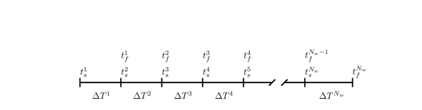
Figure 2: Partitioning of the time domain into time windows.

Over the $n$th time window, we approximate the FOM ODE solution as $\tilde{\boldsymbol{x}}^{n}(t)\approx{\boldsymbol{x}}(t)$, $t\in[t_{s}^{n},t_{f}^{n}]$, which is enforced to reside in the $n$th space–time trial subspace $\mathcal{ST}^{n}$ such that

$$\tilde{\boldsymbol{x}}^{n}\in\mathcal{ST}^{n}\subseteq\mathbb{R}^{N}\otimes\mathcal{T}^{n},\qquad n=1,\ldots,N_{w},$$ (3.1)

where $\mathcal{T}^{n}$ denotes the set of (sufficiently smooth) real-valued functions acting on $[t_{s}^{n},t_{f}^{n}]$ (i.e., $\mathcal{T}^{n}=\{f\,|\,f:[t_{s}^{n},t_{f}^{n}]\rightarrow\mathbb{R}\}$). For notational purposes, we additionally define the spatial trial subspaces at the start of each window as

$$\mathcal{B}^{n}\vcentcolon=\mathrm{span}(\{\boldsymbol{y}(t_{s}^{n})\,|\,\boldsymbol{y}\in\mathcal{ST}^{n}\})\subseteq\mathbb{R}^{N},\qquad n=1,\ldots,N_{w},$$ (3.2)

such that $\tilde{\boldsymbol{x}}^{n}(t_{s}^{n})\in\mathcal{B}^{n}$. To outline WLS, we now define the objective functional over the $n$th window as

$$\begin{split}\mathcal{J}^{n}&\vcentcolon\boldsymbol{y}\mapsto\frac{1}{2}\int_{t_{s}^{n}}^{t_{f}^{n}}\big{[}\dot{\boldsymbol{y}}(t)-\boldsymbol{f}(\boldsymbol{y}(t),t)\big{]}^{T}\mathbf{A}^{n}\big{[}\dot{\boldsymbol{y}}(t)-\boldsymbol{f}(\boldsymbol{y}(t),t)\big{]}dt,\\ &\vcentcolon\mathbb{R}^{N}\otimes\mathcal{T}^{n}\rightarrow\mathbb{R}_{+},\end{split}$$ (3.3)

where $\mathbf{A}^{n}\equiv[\mathbf{W}^{n}]^{T}\mathbf{W}^{n}\in\mathbb{R}^{N\times N}$ denotes a symmetric positive semi-definite matrix that can enable hyper-reduction, for example.

The WLS approach sequentially computes approximate solutions $\tilde{\boldsymbol{x}}^{n}\in\mathcal{ST}^{n}$, $n=1,\ldots,N_{w}$, where $\tilde{\boldsymbol{x}}^{n}$ is the solution to the minimization problem

$$\begin{split}&\underset{\boldsymbol{y}\in\mathcal{ST}^{n}}{\text{minimize}}\;\mathcal{J}^{n}(\boldsymbol{y}),\\ &\text{subject to }\;\boldsymbol{y}(t_{s}^{n})=\begin{cases}\mathbb{P}^{n}(\tilde{\boldsymbol{x}}^{n-1}(t_{f}^{n-1}))&n=2,\ldots,N_{w},\\ \mathbb{P}^{n}({{\mathbf{x}}_{0}})&n=1,\end{cases}\end{split}$$ (3.4)

where $\mathbb{P}^{n}:\mathbb{R}^{N}\rightarrow\mathcal{B}^{n}$ is a (spatial) projection operator onto the start of the $n$th trial space (e.g., $\ell^{2}$-orthogonal projection operator).

We now define the trial subspaces $\mathcal{ST}^{n}$ considered in this work. In particular, we introduce S-reduction trial subspaces and ST-reduction trial subspaces tailored for this context. We leave further investigation into other approaches, such as nonlinear trial manifolds [40], as a subject for future work.

3.2 S-reduction trial subspaces

In this context, the S-reduction trial subspace over the $n$th time window approximates the FOM ODE solution trajectory ${\boldsymbol{x}}(t)$, $t\in[t_{s}^{n},t_{f}^{n}]$ with $\tilde{\boldsymbol{x}}^{n}\in\mathcal{ST}_{\text{S}}^{n}$, where

$$\mathcal{ST}_{\text{S}}^{n}\vcentcolon=\mathcal{V}^{n}\otimes\mathcal{T}^{n}+\mathbf{x}_{\text{ref}}^{n}\otimes\mathcal{O}^{n}\subseteq\mathbb{R}^{N}\otimes\mathcal{T}^{n}.$$ (3.5)

Here, the spatial trial subspaces $\mathcal{V}^{n}\subseteq\mathbb{R}^{N}$, $n=1,\ldots,N_{w}$ satisfy $\mathcal{V}^{n}\vcentcolon=\mathrm{Ran}(\mathbf{V}^{n})$ with $\mathbf{V}^{n}\equiv[\mathbf{v}^{n}_{1}\ \cdots\ \mathbf{v}^{n}_{K^{n}}]\in\mathbb{V}_{K^{n}}(\mathbb{R}^{N})$, the reference states $\mathbf{x}_{\text{ref}}^{n}\in\mathbb{R}^{N}$, $n=1,\ldots,N_{w}$ provide the affine transformation, and $\mathcal{O}^{n}\in\mathcal{T}^{n}$ is defined as $\mathcal{O}^{n}:\tau\mapsto 1.$ Thus, at any time instance $t\in[t_{s}^{n},t_{f}^{n}]$, the S-reduction trial subspace approximates the FOM ODE solution as

$${\boldsymbol{x}}(t)\approx\tilde{\boldsymbol{x}}^{n}(t)=\mathbf{V}^{n}\hat{\boldsymbol{x}}^{n}(t)+\mathbf{x}_{\text{ref}}^{n},$$ (3.6)

where $\hat{\boldsymbol{x}}^{n}\in\mathbb{R}^{K^{n}}\otimes\mathcal{T}^{n}$ with $\hat{\boldsymbol{x}}^{n}:\tau\mapsto\hat{\boldsymbol{x}}^{n}(\tau)$ denotes the generalized coordinates over the $n$th time window.

Setting $\mathcal{ST}^{n}\leftarrow\mathcal{ST}_{\text{S}}^{n}$ in the WLS minimization problem (3.4) and setting $\mathbb{P}^{n}$ to the $\ell^{2}$-orthogonal projection operator implies that WLS with S-reduction space–time trial subspaces sequentially computes solutions $\hat{\boldsymbol{x}}^{n}$, $n=1,\ldots,N_{w}$ that satisfy

$$\begin{split}&\underset{\hat{\boldsymbol{y}}\in\mathbb{R}^{K^{n}}\otimes\mathcal{T}^{n}}{\text{minimize}}\;\mathcal{J}^{n}(\mathbf{V}^{n}\hat{\boldsymbol{y}}+\mathbf{x}_{\text{ref}}^{n}\otimes\mathcal{O}^{n}),\\ &\text{subject to }\;\hat{\boldsymbol{y}}(t_{s}^{n})=\begin{cases}[\mathbf{V}^{n}]^{T}(\mathbf{V}^{n-1}\hat{\boldsymbol{x}}^{n-1}(t_{f}^{n-1})+\mathbf{x}_{\text{ref}}^{n-1}-\mathbf{x}_{\text{ref}}^{n})&n=2,\ldots,N_{w},\\ [\mathbf{V}^{1}]^{T}({{\mathbf{x}}_{0}}-\mathbf{x}_{\text{ref}}^{1})&n=1.\end{cases}\end{split}$$ (3.7)

3.2.1 Stationary conditions and the Euler–Lagrange equations

We derive stationary conditions for optimization problem (3.7) via the Euler–Lagrange equations from the calculus of variations. To begin, we define the integrand appearing in the objective function $\mathcal{J}^{n}$ defined in Eq. (3.3) in terms of the generalized coordinates induced by the S-reduction subspace as

$$\begin{split}\mathcal{I}^{n}&\vcentcolon(\hat{\mathbf{y}},\hat{\mathbf{v}},\tau)\mapsto\frac{1}{2}\big{[}\mathbf{V}^{n}\hat{\mathbf{v}}-\boldsymbol{f}(\mathbf{V}^{n}\hat{\mathbf{y}}+\mathbf{x}_{\text{ref}}^{n},\tau)\big{]}^{T}\mathbf{A}^{n}\big{[}\mathbf{V}^{n}\hat{\mathbf{v}}-\boldsymbol{f}(\mathbf{V}^{n}\hat{\mathbf{y}}+\mathbf{x}_{\text{ref}}^{n},\tau)\big{]},\\ &\vcentcolon\mathbb{R}^{K^{n}}\times\mathbb{R}^{K^{n}}\times[t_{s}^{n},t_{f}^{n}]\rightarrow\mathbb{R}_{+}.\end{split}$$ (3.8)

We also define the quantities

$$\begin{split}\mathcal{I}_{\hat{\mathbf{v}}}^{n}&\vcentcolon(\hat{\boldsymbol{y}},\hat{\boldsymbol{v}},\tau)\mapsto\bigg{[}\frac{\partial\mathcal{I}^{n}}{\partial\hat{\mathbf{v}}}(\hat{\boldsymbol{y}}(\tau),\hat{\boldsymbol{v}}(\tau),\tau)\bigg{]}^{T},\\ &\vcentcolon\mathbb{R}^{K^{n}}\otimes\mathcal{T}^{n}\times\mathbb{R}^{K^{n}}\otimes\mathcal{T}^{n}\times[t_{s}^{n},t_{f}^{n}]\rightarrow\mathbb{R}^{K^{n}},\end{split}$$ (3.9)

$$\begin{split}\mathcal{I}_{\hat{\mathbf{y}}}^{n}&\vcentcolon(\hat{\boldsymbol{y}},\hat{\boldsymbol{v}},\tau)\mapsto\bigg{[}\frac{\partial\mathcal{I}^{n}}{\partial\hat{\mathbf{y}}}(\hat{\boldsymbol{y}}(\tau),\hat{\boldsymbol{v}}(\tau),\tau)\bigg{]}^{T},\\ &\vcentcolon\mathbb{R}^{K^{n}}\otimes\mathcal{T}^{n}\times\mathbb{R}^{K^{n}}\otimes\mathcal{T}^{n}\times[t_{s}^{n},t_{f}^{n}]\rightarrow\mathbb{R}^{K^{n}}.\end{split}$$ (3.10)

Using this notation, the Euler–Lagrange equations (see Appendix C for the derivation) over the $n$th time window for $t\in[t_{s}^{n},t_{f}^{n}]$ are given by

$$\begin{split}&\mathcal{I}_{\hat{\mathbf{y}}}^{n}(\hat{\boldsymbol{x}}^{n},\dot{\hat{\boldsymbol{x}}}^{n},t)-\dot{\mathcal{I}}_{\hat{\mathbf{v}}}^{n}(\hat{\boldsymbol{x}}^{n},\dot{\hat{\boldsymbol{x}}}^{n},t)=\boldsymbol{0},\\ &\hat{\boldsymbol{x}}^{n}(t_{s}^{n})=\begin{cases}[\mathbf{V}^{n}]^{T}(\mathbf{V}^{n-1}\hat{\boldsymbol{x}}^{n-1}(t_{f}^{n-1})+\mathbf{x}_{\text{ref}}^{n-1}-\mathbf{x}_{\text{ref}}^{n})&n=2,\ldots,N_{w},\\ [\mathbf{V}^{1}]^{T}({{\mathbf{x}}_{0}}-\mathbf{x}_{\text{ref}}^{1})&n=1,\end{cases}\\ &\mathcal{I}_{\hat{\mathbf{v}}}^{n}(\hat{\boldsymbol{x}}^{n},\dot{\hat{\boldsymbol{x}}}^{n},t_{f}^{n})=\boldsymbol{0}.\end{split}$$ (3.11)

Appendix D provides the steps required to evaluate the terms in system (3.11); the resulting system can be written as the following coupled forward–backward system for $t\in[t_{s}^{n},t_{f}^{n}]$:

$$\mathbf{M}^{n}\dot{\hat{\boldsymbol{x}}}^{n}(t)-[\mathbf{V}^{n}]^{T}\mathbf{A}^{n}\boldsymbol{f}(\mathbf{V}^{n}\hat{\boldsymbol{x}}^{n}(t)+\mathbf{x}_{\text{ref}}^{n},t)=\mathbf{M}^{n}\hat{\boldsymbol{\lambda}}^{n}(t),$$ (3.12)

$$\begin{split}&\mathbf{M}^{n}\dot{\hat{\boldsymbol{\lambda}}}^{n}(t)+[\mathbf{V}^{n}]^{T}\bigg{[}\frac{\partial\boldsymbol{f}}{\partial\mathbf{y}}(\mathbf{V}^{n}\hat{\boldsymbol{x}}^{n}(t)+\mathbf{x}_{\text{ref}}^{n},t)\bigg{]}^{T}\mathbf{A}^{n}\mathbf{V}^{n}\hat{\boldsymbol{\lambda}}^{n}(t)=-[\mathbf{V}^{n}]^{T}\big{[}\frac{\partial\boldsymbol{f}}{\partial\mathbf{y}}(\mathbf{V}^{n}\hat{\boldsymbol{x}}^{n}(t)+\mathbf{x}_{\text{ref}}^{n},t)\big{]}^{T}\\ &\hskip 122.85876pt\mathbf{A}^{n}\big{(}\mathbf{I}-\mathbf{V}^{n}[\mathbf{M}^{n}]^{-1}[\mathbf{V}^{n}]^{T}\mathbf{A}^{n}\big{)}\big{(}\mathbf{V}^{n}\dot{\hat{\boldsymbol{x}}}^{n}(t)-\boldsymbol{f}(\mathbf{V}^{n}\hat{\boldsymbol{x}}^{n}(t)+\mathbf{x}_{\text{ref}}^{n},t)\big{)},\end{split}$$ (3.13)

$$\hat{\boldsymbol{x}}^{n}(t_{s}^{n})=\begin{cases}[\mathbf{V}^{n}]^{T}(\mathbf{V}^{n-1}\hat{\boldsymbol{x}}^{n-1}(t_{f}^{n-1})+\mathbf{x}_{\text{ref}}^{n-1}-\mathbf{x}_{\text{ref}}^{n})&n=2,\ldots,N_{w},\\ [\mathbf{V}^{1}]^{T}({{\mathbf{x}}_{0}}-\mathbf{x}_{\text{ref}}^{1})&n=1,\end{cases}$$ (3.14)

$$\hat{\boldsymbol{\lambda}}^{n}(t_{f}^{n})=\boldsymbol{0},$$ (3.15)

where

$$\begin{split}\hat{\boldsymbol{\lambda}}^{n}&:\tau\mapsto\dot{\hat{\boldsymbol{x}}}^{n}(\tau)-[\mathbf{M}^{n}]^{-1}[\mathbf{V}^{n}]^{T}\mathbf{A}^{n}\boldsymbol{f}(\mathbf{V}^{n}\hat{\boldsymbol{x}}^{n}(\tau)+\mathbf{x}_{\text{ref}}^{n},\tau),\\ &:[t_{s}^{n},t_{f}^{n}]\rightarrow\mathbb{R}^{K^{n}},\end{split}$$ (3.16)

is the adjoint or “costate” variable with $\dot{\hat{\boldsymbol{\lambda}}}^{n}\equiv d\hat{\boldsymbol{\lambda}}^{n}/d\tau$, and $\mathbf{M}^{n}\equiv[\mathbf{V}^{n}]^{T}\mathbf{A}^{n}\mathbf{V}^{n}$ is a mass matrix. Eq. (3.12) is equivalent to a Galerkin reduced-order model forced by the costate variable $\hat{\boldsymbol{\lambda}}^{n}$. Eq. (3.13) is typically referred to as the adjoint equation, which is linear in the costate and is forced by the residual. We note that both ODEs (3.12) and (3.13) can be equipped with hyper-reduction, e.g., via collocation, (discrete) empirical interpolation, Gappy POD [30, 3, 28]. The state–costate coupled system (3.12)–(3.15) can be interpreted as an “optimally controlled” ROM, wherein the adjoint equation controls the forward model by enforcing the minimum residual condition over the time window.

We note that in the case $\mathbf{A}^{n}=\mathbf{I}$, the system simplifies to

$$\dot{\hat{\boldsymbol{x}}}^{n}(t)-[\mathbf{V}^{n}]^{T}\boldsymbol{f}(\mathbf{V}^{n}\hat{\boldsymbol{x}}^{n}(t)+\mathbf{x}_{\text{ref}}^{n},t)=\hat{\boldsymbol{\lambda}}^{n}(t),$$

$$\dot{\hat{\boldsymbol{\lambda}}}^{n}(t)+[\mathbf{V}^{n}]^{T}\bigg{[}\frac{\partial\boldsymbol{f}}{\partial\mathbf{y}}(\mathbf{V}^{n}\hat{\boldsymbol{x}}^{n}(t)+\mathbf{x}_{\text{ref}}^{n},t)\bigg{]}^{T}\mathbf{V}^{n}\hat{\boldsymbol{\lambda}}^{n}(t)=$$

$$\hskip 144.54pt[\mathbf{V}^{n}]^{T}\bigg{[}\frac{\partial\boldsymbol{f}}{\partial\mathbf{y}}(\mathbf{V}^{n}\hat{\boldsymbol{x}}^{n}(t)+\mathbf{x}_{\text{ref}}^{n},t)\bigg{]}^{T}\big{(}\mathbf{I}-\mathbf{V}^{n}[\mathbf{V}^{n}]^{T}\big{)}\boldsymbol{f}(\mathbf{V}^{n}\hat{\boldsymbol{x}}^{n}(t)+\mathbf{x}_{\text{ref}}^{n},t),$$

$$\hat{\boldsymbol{x}}^{n}(t_{s}^{n})=\begin{cases}[\mathbf{V}^{n}]^{T}(\mathbf{V}^{n-1}\hat{\boldsymbol{x}}^{n-1}(t_{f}^{n-1})-\mathbf{x}_{\text{ref}}^{n})&n=2,\ldots,N_{w},\\ [\mathbf{V}^{1}]^{T}({{\mathbf{x}}_{0}}-\mathbf{x}_{\text{ref}}^{1})&n=1,\end{cases}$$

$$\hat{\boldsymbol{\lambda}}^{n}(t_{f}^{n})=\boldsymbol{0}.$$

3.2.2 Formulation as an optimal-control problem of Lagrange type

The stationary conditions for WLS with S-reduction trial subspaces (3.12)–(3.15) can be alternatively formulated as a Lagrange problem from optimal control. To this end, recall the dynamics of the Galerkin ROM over $t\in[t_{s}^{n},t_{f}^{n}]$,

$$[\mathbf{V}]^{T}\mathbf{A}\mathbf{V}\dot{\hat{\boldsymbol{x}}}_{\text{G}}(t)-[\mathbf{V}]^{T}\mathbf{A}\boldsymbol{f}(\mathbf{V}\hat{\boldsymbol{x}}_{\text{G}}+\mathbf{x}_{\text{ref}},t)=\boldsymbol{0}.$$

We introduce now a controller ${\hat{\boldsymbol{u}}^{n}}\in\mathbb{R}^{K^{n}}\otimes\mathcal{T}^{n}$ and pose the problem of finding a controller that minimizes the residual over the time window and forces the dynamics as

$$[\mathbf{V}^{n}]^{T}\mathbf{A}^{n}\mathbf{V}^{n}\dot{\hat{\boldsymbol{x}}}^{n}(t)-[\mathbf{V}^{n}]^{T}\mathbf{A}^{n}\boldsymbol{f}(\mathbf{V}^{n}\hat{\boldsymbol{x}}^{n}(t)+\mathbf{x}_{\text{ref}}^{n},t)=\hat{\boldsymbol{u}}^{n}(t).$$ (3.17)

We now demonstrate how to compute this controller. Before doing so, we note that (3.17) displays commonalities with subgrid-scale methods [58, 35, 15, 50, 67, 65, 60], which add an additional term to the reduced-order model in order to account for truncated states.

We begin by defining a Lagrangian

$$\begin{split}\mathcal{L}^{n}&:(\hat{\mathbf{y}},\hat{\mathbf{v}},\tau)\mapsto\frac{1}{2}\bigg{[}\mathbf{V}^{n}\bigg{(}[\mathbf{M}^{n}]^{-1}[\mathbf{V}^{n}]^{T}\mathbf{A}^{n}\boldsymbol{f}(\mathbf{V}^{n}\hat{\mathbf{y}}+\mathbf{x}_{\text{ref}}^{n},\tau)+[\mathbf{M}^{n}]^{-1}\hat{\mathbf{v}}\bigg{)}-\boldsymbol{f}(\mathbf{V}^{n}\hat{\mathbf{y}}+\mathbf{x}_{\text{ref}}^{n},\tau)\bigg{]}^{T}\mathbf{A}^{n}\\ &\hskip 108.405pt\bigg{[}\mathbf{V}^{n}\bigg{(}[\mathbf{M}^{n}]^{-1}[\mathbf{V}^{n}]^{T}\mathbf{A}^{n}\boldsymbol{f}(\mathbf{V}^{n}\hat{\mathbf{y}}+\mathbf{x}_{\text{ref}}^{n},\tau)+[\mathbf{M}^{n}]^{-1}\hat{\mathbf{v}}\bigg{)}-\boldsymbol{f}(\mathbf{V}^{n}\hat{\mathbf{y}}+\mathbf{x}_{\text{ref}}^{n},\tau)\bigg{]},\\ &:\mathbb{R}^{K^{n}}\times\mathbb{R}^{K^{n}}\times[t_{s}^{n},t_{f}^{n}]\rightarrow\mathbb{R}_{+}{},\end{split}$$

where we have used $\dot{\hat{\boldsymbol{x}}}^{n}(t)=[\mathbf{M}^{n}]^{-1}[\mathbf{V}^{n}]^{T}\mathbf{A}^{n}\boldsymbol{f}(\mathbf{V}^{n}\hat{\boldsymbol{x}}^{n}(t)+\mathbf{x}_{\text{ref}}^{n},t)+[\mathbf{M}^{n}]^{-1}\hat{\boldsymbol{u}}^{n}(t)$ from Eq. (3.17). Note that this Lagrangian measures the same residual as Eq. (3.8). The WLS approach with S-reduction trial subspaces can be formulated as an optimal-control method that sequentially computes the controllers ${\hat{\boldsymbol{u}}^{n}}\in\mathbb{R}^{K^{n}}\otimes\mathcal{T}^{n}$, $n=1,\ldots,N_{w}$ that satisfy

$$\begin{split}&\underset{\hat{\boldsymbol{v}}\in\mathbb{R}^{K^{n}}\otimes\mathcal{T}^{n}}{\text{minimize }}\int_{t_{s}^{n}}^{t_{f}^{n}}\mathcal{L}^{n}(\hat{\boldsymbol{x}}^{n}(t),\hat{\boldsymbol{v}}(t),t)dt,\\ &\text{subject to }\;\left\{\begin{array}[]{l}[\mathbf{V}^{n}]^{T}\mathbf{A}^{n}\mathbf{V}^{n}\dot{\hat{\boldsymbol{x}}}^{n}(t)-[\mathbf{V}^{n}]^{T}\mathbf{A}^{n}\boldsymbol{f}(\mathbf{V}^{n}\hat{\boldsymbol{x}}^{n}(t)+\mathbf{x}_{\text{ref}}^{n},t)=\hat{\boldsymbol{v}}(t),\quad t\in[t_{s}^{n},t_{f}^{n}]\\ \hat{\boldsymbol{x}}^{n}(t_{s}^{n})=\begin{cases}[\mathbf{V}^{n}]^{T}(\mathbf{V}^{n-1}\hat{\boldsymbol{x}}^{n-1}(t_{f}^{n-1})+\mathbf{x}_{\text{ref}}^{n-1}-\mathbf{x}_{\text{ref}}^{n})&n=2,\ldots,N_{w},\\ [\mathbf{V}^{1}]^{T}({{\mathbf{x}}_{0}}-\mathbf{x}_{\text{ref}}^{1})&n=1.\end{cases}\end{array}\right.\end{split}$$ (3.18)

The solution to the system (3.18) is equivalent of that defined by (3.7). This can be demonstrated via the Pontryagin Maximum Principle (PMP) [37]. To this end, we introduce the Lagrange multiplier (costate) $\hat{\boldsymbol{\nu}}^{n}\in\mathbb{R}^{K^{n}}\otimes\mathcal{T}^{n}$ and define the Hamiltonian

$$\begin{split}\mathcal{H}^{n}\;&:\;(\hat{\mathbf{y}},\hat{\boldsymbol{\mu}},\hat{\mathbf{v}},\tau)\mapsto\hat{\boldsymbol{\mu}}^{T}\bigg{[}[\mathbf{M}^{n}]^{-1}[\mathbf{V}^{n}]^{T}\mathbf{A}^{n}\boldsymbol{f}(\mathbf{V}^{n}\hat{\mathbf{y}}+\mathbf{x}_{\text{ref}}^{n},\tau)+[\mathbf{M}^{n}]^{-1}\hat{\mathbf{v}}\bigg{]}+\mathcal{L}^{n}(\hat{\mathbf{y}},\hat{\mathbf{v}},\tau),\\ &:\;\mathbb{R}^{K^{n}}\times\mathbb{R}^{K^{n}}\times\mathbb{R}^{K^{n}}\times[t_{s}^{n},t_{f}^{n}]\rightarrow\mathbb{R}.\end{split}$$ (3.19)

The Pontryagin Maximum Principle states that solutions of the optimization problem (3.18) must satisfy the following conditions over the $n$th window,

$$\dot{\hat{\boldsymbol{x}}}^{n}(t)=\frac{\partial\mathcal{H}^{n}}{\partial\hat{\boldsymbol{\mu}}{}}(\hat{\boldsymbol{x}}^{n}(t),\hat{\boldsymbol{\nu}}^{n}(t),\hat{\boldsymbol{u}}^{n}(t),t),$$

$$\dot{\hat{\boldsymbol{\nu}}}^{n}(t)=-\frac{\partial\mathcal{H}^{n}}{\partial\hat{\mathbf{y}}{}}(\hat{\boldsymbol{x}}^{n}(t),\hat{\boldsymbol{\nu}}^{n}(t),\hat{\boldsymbol{u}}^{n}(t),t),$$

$$\frac{\partial\mathcal{H}^{n}}{\partial\hat{\mathbf{v}}{}}(\hat{\boldsymbol{x}}^{n}(t),\hat{\boldsymbol{\nu}}^{n}(t),\hat{\boldsymbol{u}}^{n}(t),t)=\boldsymbol{0},$$

$$\hat{\boldsymbol{x}}^{n}(t_{s}^{n})=\begin{cases}[\mathbf{V}^{n}]^{T}(\mathbf{V}^{n-1}\hat{\boldsymbol{x}}^{n-1}(t_{f}^{n-1})+\mathbf{x}_{\text{ref}}^{n-1}-\mathbf{x}_{\text{ref}}^{n})&n=2,\ldots,N_{w},\\ [\mathbf{V}^{1}]^{T}({{\mathbf{x}}_{0}}-\mathbf{x}_{\text{ref}}^{1})&n=1,\end{cases}$$

$$\hat{\boldsymbol{\nu}}^{n}(t_{f}^{n})=\boldsymbol{0}.$$

Evaluation of the required gradients (Appendix E) yields the system to be solved over the $n$th window for $t\in[t_{s}^{n},t_{f}^{n}]$,

$$\begin{split}&\mathbf{M}^{n}\dot{\hat{\boldsymbol{x}}}^{n}(t)-[\mathbf{V}^{n}]^{T}\mathbf{A}^{n}\boldsymbol{f}(\mathbf{V}^{n}\hat{\boldsymbol{x}}^{n}(t)+\mathbf{x}_{\text{ref}}^{n},t)=\hat{\boldsymbol{u}}^{n}(t),\\ &\dot{\hat{\boldsymbol{\nu}}}^{n}(t)+[\mathbf{V}^{n}]^{T}\bigg{[}\frac{\partial\boldsymbol{f}}{\partial\mathbf{y}}(\mathbf{V}^{n}\hat{\boldsymbol{x}}^{n}(t)+\mathbf{x}_{\text{ref}}^{n},t)\bigg{]}^{T}\mathbf{A}^{n}\mathbf{V}^{n}[\mathbf{M}^{n}]^{-1}\hat{\boldsymbol{\nu}}^{n}(t)=[\mathbf{V}^{n}]^{T}\big{[}\frac{\partial\boldsymbol{f}}{\partial\mathbf{y}}(\mathbf{V}^{n}\hat{\boldsymbol{x}}^{n}(t)+\mathbf{x}_{\text{ref}}^{n},t)\big{]}^{T}\\ &\hskip 130.08621pt\mathbf{A}^{n}\big{(}\mathbf{I}-\mathbf{V}^{n}[\mathbf{M}^{n}]^{-1}[\mathbf{V}^{n}]^{T}\mathbf{A}^{n}\big{)}\big{(}\mathbf{V}^{n}\dot{\hat{\boldsymbol{x}}}^{n}(t)-\boldsymbol{f}(\mathbf{V}^{n}\hat{\boldsymbol{x}}^{n}(t)+\mathbf{x}_{\text{ref}}^{n},t)\big{)},\\ &\hat{\boldsymbol{u}}^{n}(t)=-\hat{\boldsymbol{\nu}}^{n}(t),\\ &\hat{\boldsymbol{x}}^{n}(t_{s}^{n})=\begin{cases}[\mathbf{V}^{n}]^{T}(\mathbf{V}^{n-1}\hat{\boldsymbol{x}}^{n-1}(t_{f}^{n-1})+\mathbf{x}_{\text{ref}}^{n-1}-\mathbf{x}_{\text{ref}}^{n})&n=2,\ldots,N_{w},\\ [\mathbf{V}^{1}]^{T}({{\mathbf{x}}_{0}}-\mathbf{x}_{\text{ref}}^{1})&n=1,\end{cases}\\ &\hat{\boldsymbol{\nu}}^{n}(t_{f}^{n})=\boldsymbol{0}.\\ \end{split}$$ (3.20)

Setting ${\hat{\boldsymbol{u}}^{n}}=\mathbf{M}^{n}\hat{\boldsymbol{\lambda}}^{n}$ and $\hat{\boldsymbol{\nu}}^{n}=-\mathbf{M}^{n}\hat{\boldsymbol{\lambda}}^{n}$ results in equivalence between the system (3.20) and the system (3.12)–(3.15). Thus, WLS with S-reduction trial subspaces can be formulated as an optimal control problem: WLS computes a controller that modifies the Galerkin ROM to minimize the residual over the time window. The WLS method can additionally be interpreted as a subgrid-scale modeling technique that constructs a residual-minimizing subgrid-scale model.

Remark 3.1.

The Euler–Lagrange equations comprise a Hamiltonian system. This imbues WLS with S-reduction trial subspaces with certain properties; e.g., for autonomous systems the Hamiltonian (3.19) is conserved.

3.3 ST-reduction trial spaces

The ST-reduction trial subspace over the $n$th time window approximates the FOM ODE solution trajectory ${\boldsymbol{x}}\in\mathbb{R}^{N}\otimes\mathcal{T}$ with $\tilde{\boldsymbol{x}}^{n}\in\mathcal{ST}_{\text{ST}}^{n}$, where

$$\mathcal{ST}_{\text{ST}}^{n}\vcentcolon=\mathrm{Ran}(\boldsymbol{\Pi}^{n})+\mathbf{x}_{\text{st}}^{n}\otimes\mathcal{O}^{n}\subseteq\mathbb{R}^{N}\otimes\mathcal{T}^{n}.$$ (3.21)

Here $\boldsymbol{\Pi}^{n}\in\mathbb{R}^{N\times K_{\text{ST}}^{n}}\otimes\mathcal{T}^{n}$, $n=1,\ldots,N_{w}$, with $\boldsymbol{\Pi}^{n}:\tau\mapsto\boldsymbol{\Pi}^{n}(\tau)$ and $\boldsymbol{\Pi}^{n}(t_{s}^{n})=\boldsymbol{0}$ is the space–time trial basis matrix function and $\mathbf{x}_{\text{st}}^{n}\in\mathbb{R}^{N}$, $n=1,\ldots,N_{w}$ provides the affine transformation. To enforce the initial condition and ensure solution continuity across time windows, we set $\mathbf{x}_{\text{st}}^{1}={{\mathbf{x}}_{0}}$ and $\mathbf{x}_{\text{st}}^{n}=\tilde{\boldsymbol{x}}^{n-1}(t_{f}^{n-1})$ for $n=2,\ldots,N_{w}$. At any time instance $t\in[t_{s}^{n},t_{f}^{n}]$, the ST-reduction trial subspace approximates the FOM ODE solution as

$${\boldsymbol{x}}^{n}(t)\approx\tilde{\boldsymbol{x}}^{n}(t)=\boldsymbol{\Pi}^{n}(t)\hat{\mathbf{\overline{x}}}^{n}+\mathbf{x}_{\text{st}}^{n},$$ (3.22)

where $\hat{\mathbf{\overline{x}}}^{n}\in\mathbb{R}^{K_{\text{ST}}^{n}}$ are the space–time generalized coordinates over the $n$th window. Setting $\mathcal{ST}^{n}\leftarrow\mathcal{ST}_{\text{ST}}^{n}$ in the WLS minimization problem (3.4) implies that WLS with ST-reduction trial subspaces sequentially computes solutions $\hat{\mathbf{\overline{x}}}^{n}$, $n=1,\ldots,N_{w}$ that satisfy

$$\begin{split}&\underset{\hat{\mathbf{\overline{y}}}\in\mathbb{R}^{K_{\text{ST}}^{n}}}{\text{minimize}}\;\mathcal{J}^{n}(\boldsymbol{\Pi}^{n}\hat{\mathbf{\overline{y}}}+\mathbf{x}_{\text{st}}^{n}\otimes\mathcal{O}^{n}).\end{split}$$ (3.23)

3.3.1 Stationary conditions

The key difference between ST-reduction and S-reduction trial subspaces is as follows: generalized coordinates for ST-reduction trial subspaces comprise a vector in $\mathbb{R}^{K_{\text{ST}}^{n}}$, while generalized coordinates for the S-reduction trial subspaces comprise a time-dependent vector in $\mathbb{R}^{K^{n}}\otimes\mathcal{T}^{n}$. Thus, in the ST-reduction case, the optimization problem is no longer minimizing a functional with respect to a (time-dependent) function, but is minimizing a function with respect to a vector. As such, the first-order optimality conditions can be derived using standard calculus. Differentiating the objective function with respect to the generalized coordinates and setting the result equal to zero yields

$$\int_{t_{s}^{n}}^{t_{f}^{n}}\bigg{[}\dot{\boldsymbol{\Pi}}^{n}(t)^{T}-\boldsymbol{\Pi}^{n}(t)^{T}\bigg{[}\frac{\partial\boldsymbol{f}}{\partial\mathbf{y}}(\dot{\boldsymbol{\Pi}}^{n}(t)\hat{\mathbf{\overline{x}}}^{n}+\mathbf{x}_{\text{st}}^{n},t)\bigg{]}^{T}\bigg{]}\mathbf{A}^{n}\bigg{(}\dot{\boldsymbol{\Pi}}^{n}(t)\hat{\mathbf{\overline{x}}}^{n}-\boldsymbol{f}(\boldsymbol{\Pi}^{n}(t)\hat{\mathbf{\overline{x}}}^{n}+\mathbf{x}_{\text{st}}^{n},t)\bigg{)}dt=\boldsymbol{0}.$$ (3.24)

Thus, for ST-reduction trial subspaces, the stationary conditions comprise a system of algebraic equations, as opposed to a system of differential equations as with S-reduction trial subspaces.

3.4 WLS summary

This section outlined the WLS approach for model reduction. In summary, WLS sequentially minimizes the time continuous FOM ODE residual within the range of a space–time trial subspace over time windows; i.e., WLS sequentially computes approximate solutions $\tilde{\boldsymbol{x}}^{n}\in\mathcal{ST}^{n}$, $n=1,\ldots,N_{w}$ that comprise solutions to the optimization problem (3.4). For S-reduction trial subspaces, the stationary conditions for the residual minimization problem can be derived via the Euler–Lagrange equations and yield the system (3.12)–(3.15) over the $n$th window for $t\in[t_{s}^{n},t_{f}^{n}]$. WLS with S-reduction trial subspaces can be alternatively interpreted as a Lagrange problem from optimal control: the Galerkin method is forced by a controller that enforces the residual minimization property. Section 3.3 additionally considered ST-reduction trial subspaces. For ST-reduction trial subspaces, in where the generalized coordinates are no longer functions, the stationary conditions correspond to the system of algebraic equations (3.24).

4 Numerical solution techniques

We now consider numerical-solution techniques for the WLS approach. We focus primarily on direct (i.e., discretize-then-optimize) and indirect (i.e., optimize-then-discretize) methods for S-reduction trial subspaces, and then briefly outline direct and indirect methods for ST-reduction trial subspaces.

4.1 S-reduction: direct and indirect methods

WLS with S-reduction trial subspaces can be viewed as an optimal-control problem. Numerical solution techniques for optimal-control problems can be classified as either direct or indirect methods [27]. Rather than working with the first-order optimality conditions (3.12)–(3.15), direct methods “directly” solve the optimization problem (3.4) by first numerically discretizing the objective functional and “transcribing” the infinite-dimensional problem into a finite-dimensional problem. Direct approaches thus “discretize then optimize”. In contrast, indirect methods compute solutions to the Euler–Lagrange equations (3.12)–(3.15) (which comprise the first-order optimality conditions). Thus, indirect methods “optimize then discretize,” and solve the optimization problem “indirectly.” A variety of both discretization and solution techniques are possible for both direct and indirect methods. Collocation methods, finite-element methods, spectral methods, and shooting methods are all examples of possible solution techniques.

In the present context, we investigate both direct and indirect methods to solve WLS with S-reduction trial subspaces. In particular, we consider:

• Direct methods (discretize then optimize): A direct approach that leverages linear multistep methods to directly solve the optimization problem (3.7). Section 4.2 outlines this approach.

• Indirect methods (optimize then discretize): An indirect approach that leverages the forward–backward sweep algorithm to solve the Euler–Lagrange equations (3.12)–(3.15). Section 4.3 outlines this technique.

We note that a variety of other approaches exist, and their investigation comprises the subject of future work.

4.2 S-reduction trial subspaces: direct solution approach

Direct approaches solve optimization problem (3.4) by “transcribing” the infinite-dimensional optimization problem into a finite-dimensional one by discretizing the state and objective functional in time. The minimization problem is then reformulated as a (non)linear optimization problem. A variety of direct solution approaches exist, including collocation approaches, spectral methods, and genetic algorithms. In the context of S-reduction trial subspaces, the most straightforward direct solution approach consists of the following steps: (1) numerically discretize the FOM ODE (and hence the integrand of the objective function in problem (3.7)) and (2) select a numerical quadrature rule to evaluate the integral defining the objective function in (3.7). To this end, we define time grids $\{\tau^{n,i}\}_{i=0}^{N_{\tau}^{n}}\subset[t_{s}^{n},t_{f}^{n}]$, $n=1,\ldots,N_{w}$ that satisfy $t_{s}^{n}=\tau^{n,0}\leq\cdots\leq\tau^{n,N_{\tau}^{n}}=t_{f}^{n}$. Figure 3 depicts such a discretization. For the purposes of indexing between different windows, we additionally define a function:

$$\theta:(n,i)\mapsto\begin{cases}(n,i)&n=1,\;i=0,\\ (n,i)&n\geq 1,\;i>0,\\ \theta(n-1,N_{\tau}^{n-1}+i)&n>1,\;i\leq 0.\end{cases}$$

We now outline the direct solution approach for linear-multistep schemes; the formulation for other time-integration methods (e.g., Runge–Kutta) follows closely.

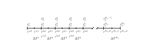
Figure 3: Depiction of the $N_{\tau}^{n}+1$ time instances over each window. In the figure, $N_{\tau}^{n}=2$ for all $n$.

4.2.1 Linear multistep schemes

Linear multistep schemes approximate the solution at time instance $\tau^{n,i}$ using the previous $k^{n,i}$ time instances, where $k^{n,i}$ denotes the number of time steps employed by the scheme at the $i$th time instance of the $n$th window. Employing such a method to discretize the FOM ODE yields the sequence of FOM O$\Delta$Es defined over the $n$th time window

$$\boldsymbol{r}^{n,i}({\mathbf{x}}^{n,i};{\mathbf{x}}^{\theta(n,i-1)},\ldots,{\mathbf{x}}^{\theta(n,i-k^{n,i})})=\boldsymbol{0},\qquad i=1,\ldots,N_{\tau}^{n}$$

along with the initial condition ${\mathbf{x}}^{1,0}={{\mathbf{x}}_{0}}$. Here, ${\mathbf{x}}^{n,i}(\approx{\boldsymbol{x}}(\tau^{n,i}))\in\mathbb{R}^{N}$ and $\boldsymbol{r}^{n,i}$ denotes the FOM O$\Delta$E residual over the $i$th time instance of the $n$th window defined as

$$\boldsymbol{r}^{n,i} :(\mathbf{y}^{i};\mathbf{y}^{i-1},\ldots,\mathbf{y}^{i-k^{n,i}})\mapsto\frac{1}{\Delta t^{n,i}}\sum_{j=0}^{k^{n,i}}\alpha^{n,i}_{j}\mathbf{y}^{i-j}-\sum_{j=0}^{k^{n,i}}\beta^{n,i}_{j}\boldsymbol{f}(\mathbf{y}^{i-j},\tau^{\theta(n,i-j)}),$$

$$:\mathbb{R}^{N}\otimes\mathbb{R}^{k^{n,i}+1}\rightarrow\mathbb{R}^{N}.$$

Here, $\Delta t^{n,i}\vcentcolon=\tau^{n,i}-\tau^{n,i-1}$ denotes the time step, and $\alpha^{n,i}_{j},\beta^{n,i}_{j}\in\mathbb{R}$ denote coefficients that define the specific type of multistep scheme at the $i$th time instance of the $n$th window. Employing a linear multistep method allows the objective functional (3.3) to be replaced with the objective function

$$\begin{split}J^{n}_{\text{D}}&\vcentcolon(\mathbf{y}^{1},\ldots,\mathbf{y}^{N_{\tau}^{n}};\mathbf{y}^{0},\ldots,\mathbf{y}^{-k^{n,1}+1})\mapsto\frac{1}{2}\sum_{i=1}^{N_{\tau}^{n}}\gamma^{n,i}[\boldsymbol{r}^{n,i}(\mathbf{y}^{i};\mathbf{y}^{i-1},\ldots,\mathbf{y}^{i-k^{n,i})})]^{T}\mathbf{A}^{n}\boldsymbol{r}^{n,i}(\mathbf{y}^{i};\mathbf{y}^{i-1},\ldots,\mathbf{y}^{i-k^{n,i}}),\\ &\vcentcolon\mathbb{R}^{N}\otimes\mathbb{R}^{N_{\tau}^{n}+k^{n,1}}\rightarrow\mathbb{R}_{+},\end{split}$$

where $\gamma^{n,i}\in\mathbb{R}_{+}$ are quadrature weights.

WLS with the direct approach and a linear multistep method sequentially computes the solutions $\tilde{\mathbf{x}}^{n,1},\ldots,\tilde{\mathbf{x}}^{n,N_{\tau}^{n}}$, $n=1,\ldots,N_{w}$ that satisfy

$$\underset{(\mathbf{y}^{1},\ldots,\mathbf{y}^{N_{\tau}^{n}})\in(\mathcal{V}+\mathbf{x}_{\text{ref}}^{n})\otimes\mathbb{R}^{N_{\tau}^{n}}}{\text{minimize }}J^{n}_{\text{D}}(\mathbf{y}^{1},\ldots,\mathbf{y}^{N_{\tau}^{n}};\tilde{\mathbf{x}}^{\theta(n,0)},\ldots,\tilde{\mathbf{x}}^{\theta(n,-k^{n,1}+1)}),$$

with the initial condition $\tilde{\mathbf{x}}^{1,0}=\mathbf{V}^{n}[\mathbf{V}^{n}]^{T}({{\mathbf{x}}_{0}}-\mathbf{x}_{\text{ref}}^{n})+\mathbf{x}_{\text{ref}}^{n}$.

Equivalently, WLS with the direct approach and a linear multistep method sequentially computes the generalized coordinates $\hat{\mathbf{x}}^{n,1},\ldots,\hat{\mathbf{x}}^{n,N_{\tau}^{n}}$, $n=1,\ldots,N_{w}$ with $\hat{\mathbf{x}}^{n,i}(\approx\hat{\boldsymbol{x}}^{n}(\tau^{n,i}))\in\mathbb{R}^{K^{n}}$ that satisfy

$$\begin{split}&\underset{(\hat{\mathbf{y}}^{1},\ldots,\hat{\mathbf{y}}^{N_{\tau}^{n}})\in\mathbb{R}^{K^{n}}\otimes\mathbb{R}^{N_{\tau}^{n}}}{\text{minimize }}J^{n}_{\text{D}}(\mathbf{V}^{n}\hat{\mathbf{y}}^{1}+\mathbf{x}_{\text{ref}}^{n},\ldots,\mathbf{V}^{n}\hat{\mathbf{y}}^{N_{\tau}^{n}}+\mathbf{x}_{\text{ref}}^{n};\tilde{\mathbf{x}}^{\theta(n,0)},\ldots,\tilde{\mathbf{x}}^{\theta(n,-k^{n,1}+1)}).\end{split}$$ (4.1)

The optimization problem takes the form of a weighted least-squares problem. We emphasize that optimization problem (4.1) associates with an S-reduction trial subspace characterized by a reduction in spatial complexity, but no reduction in temporal complexity.

The minimization problem (4.1) requires specification of the quadrature weights (and hence the integration scheme used to discretize the objective functional). Typically, the same integration scheme used to discretize the FOM ODE is employed for consistency [53]; e.g., if a backward Euler method is used to discretize the FOM ODE, then a backward Euler method is the used to numerically integrate the objective functional.

Remark 4.1.

For the limiting case where $N_{\tau}^{n}=1$, $n=1,\ldots,N_{w}$ such that the window size is equivalent to the time step (i.e., $\Delta T^{n}=\tau^{n,1}-\tau^{n,0}$), uniform quadrature weights are used, a uniform trial space is employed (i.e., $\mathcal{V}^{n}=\mathcal{V}$ and $\mathbf{x}_{\text{ref}}^{n}=\mathbf{x}_{\text{ref}},n=1,\ldots,N_{w}$), the weighting matrices are taken to be $\mathbf{W}^{n}=\mathbf{W},n=1,\ldots,N_{w}$, and the time instances satisfy $\tau^{n,1}=t^{n}$, $n=1,\ldots,N_{w}$, then $\tilde{\mathbf{x}}^{n,1}=\tilde{\mathbf{x}}_{\text{L}}^{n}$, $n=1,\ldots,N_{w}$ and WLS with S-reduction trial subspaces solved via the direct approach recovers the LSPG approach.

4.2.2 Solution to the least-squares problem through the Gauss–Newton method

Problem (4.1) corresponds to a discrete least-squares problem, which is nonlinear if the full-order-model velocity $\boldsymbol{f}$ is nonlinear in its first argument. A variety of algorithms exist for solving nonlinear least-squares problems, including the Gauss–Newton method, and the Levenberg–Marquardt method. The numerical experiments presented in this work consider nonlinear dynamical systems and are solved via the Gauss–Newton method; as such, we outline this approach here.

Defining a “vectorization” function

$$\boldsymbol{v} \vcentcolon(\mathbf{y}^{1},\ldots,\mathbf{y}^{m})\mapsto\begin{bmatrix}[\mathbf{y}^{1}]^{T}&\ldots&[\mathbf{y}^{m}]^{T}\end{bmatrix}^{T},$$

$$\vcentcolon\mathbb{R}^{p}\otimes\mathbb{R}^{m}\rightarrow\mathbb{R}^{pm},$$

the vectorized generalized coordinates over the $n$th time window are defined as

$$\hat{\overline{\overline{\mathbf{x}}}}^{n}\vcentcolon=\boldsymbol{v}(\hat{\mathbf{x}}^{n,1},\ldots,\hat{\mathbf{x}}^{n,N_{\tau}^{n}}).$$

We now define the weighted space–time residual over the entire window as

$$\overline{\overline{\boldsymbol{r}}}^{n}_{\text{}}:\hat{\overline{\overline{\mathbf{y}}}}\mapsto\begin{bmatrix}\sqrt{\frac{\gamma^{n,1}}{2}}\mathbf{W}^{n}\boldsymbol{r}^{n,1}(\mathbf{V}^{n}\hat{\mathbf{y}}^{1}+\mathbf{x}_{\text{ref}}^{n};\tilde{\mathbf{x}}^{\theta(n,0)},\ldots,\tilde{\mathbf{x}}^{\theta(n,1-k^{n,1})})\\ \vdots\\ \sqrt{\frac{\gamma^{n,N_{\tau}^{n}}}{2}}\mathbf{W}^{n}\boldsymbol{r}^{n,N_{\tau}^{n}}(\mathbf{V}^{n}\hat{\mathbf{y}}^{N_{\tau}^{n}}+\mathbf{x}_{\text{ref}}^{n};\mathbf{V}^{n}\hat{\mathbf{y}}^{N_{\tau}^{n}-1}+\mathbf{x}_{\text{ref}}^{n},\ldots,\mathbf{V}^{n}\hat{\mathbf{y}}^{N_{\tau}^{n}-k^{n,N_{\tau}^{n}}}+\mathbf{x}_{\text{ref}}^{n})\\ \end{bmatrix},$$

where $\hat{\overline{\overline{\mathbf{y}}}}\equiv\boldsymbol{v}(\hat{\mathbf{y}}^{1},\ldots,\hat{\mathbf{y}}^{N_{\tau}^{n}})$ and, for $i\leq 0$,

$$\hat{\mathbf{y}}^{n,i}\equiv\begin{cases}\hat{\mathbf{x}}^{\theta(n,i)}&n=2,\ldots,N_{w},\\ [\mathbf{V}^{1}]^{T}({{\mathbf{x}}_{0}}-\mathbf{x}_{\text{ref}}^{1})&n=1.\end{cases}$$ (4.2)

We note that

$$J^{n}_{\text{D}}\bigg{(}\tilde{\mathbf{x}}^{n,1},\ldots,\tilde{\mathbf{x}}^{n,N_{\tau}^{n}};\tilde{\mathbf{x}}^{\theta(n,0)},\ldots,\tilde{\mathbf{x}}^{\theta(n,-k^{n,1}+1)}\bigg{)}=\bigg{[}\overline{\overline{\boldsymbol{r}}}^{n}_{\text{}}(\hat{\overline{\overline{\mathbf{x}}}}^{n})\bigg{]}^{T}\bigg{[}\overline{\overline{\boldsymbol{r}}}^{n}_{\text{}}(\hat{\overline{\overline{\mathbf{x}}}}^{n})\bigg{]}.$$

Using these definitions, Algorithm 1 presents the standard Gauss–Newton method. Each Gauss–Newton iteration consists of three fundamental steps: (1) compute the FOM O$\Delta$E residual given the current guess, (2) compute the Jacobian of the residual over the time window, and (3) solve the linear least-squares problem and update the guess.

The practical implementation of the Gauss–Newton algorithm requires an efficient method for computing the Jacobian of the residual over the time window ${\partial\overline{\overline{\boldsymbol{r}}}^{n}_{\text{}}}/{\partial\hat{\overline{\overline{\mathbf{y}}}}}$. For this purpose, we can leverage the fact that this Jacobian is a block lower triangular matrix with the following sparsity pattern (for $k^{n,i}=1$, $i=1,\ldots,N_{\tau}^{n}$):

$$\begin{bmatrix}[l]\leavevmode\hbox to15.4pt{\vbox to25.4pt{\text{[drawing]}}}&\\ \leavevmode\hbox to15.4pt{\vbox to25.4pt{\text{[drawing]}}}&\leavevmode\hbox to15.4pt{\vbox to25.4pt{\text{[drawing]}}}&\\ &\leavevmode\hbox to15.4pt{\vbox to25.4pt{\text{[drawing]}}}&\leavevmode\hbox to15.4pt{\vbox to25.4pt{\text{[drawing]}}}&\\ &&\ddots&\\ &&&\leavevmode\hbox to15.4pt{\vbox to25.4pt{\text{[drawing]}}}&\leavevmode\hbox to15.4pt{\vbox to25.4pt{\text{[drawing]}}}\end{bmatrix},$$

where each block comprises an $N\times K^{n}$ dense matrix. In particular, solution techniques can leverage this structure, e.g., to efficiently compute Jacobian–vector products. Another consequence of this sparsity pattern is that the normal equations arising at each Gauss–Newton iteration comprise a banded block system that can also be exploited.

Remark 4.2.

(Acceleration of the Gauss–Newton Method)
The principal cost of a Gauss–Newton method is often the formation of the Jacobian matrix. A variety of techniques aimed at reducing this computational burden exist; Jacobian-free Newton–Krylov methods [38], Broyden’s method [11] (as explored in Ref. [16], Appendix A), and frozen Jacobian approximations are several such examples. Further, the space–time formulation introduces an extra dimension for parallelization that can be exploited to future reduce the wall time. The investigation of these additional, potentially more efficient, solution algorithms is a topic of future work.

Input : tolerance, $\epsilon$; initial guess, $\hat{\mathbf{x}}^{n,1}_{0},\ldots,\hat{\mathbf{x}}^{n,N_{\tau}^{n}}_{0}$

Output : Solution to least squares problem, $\hat{\overline{\overline{\mathbf{x}}}}^{n}$

Online Steps:

$\text{converged}\leftarrow\text{false}$ $\triangleright$ Set convergence checker

$\hat{\overline{\overline{\mathbf{x}}}}^{n}_{0}\leftarrow\boldsymbol{v}(\hat{\mathbf{x}}^{n,1}_{0},\ldots,\hat{\mathbf{x}}^{n,N_{\tau}^{n}}_{0})$ $\triangleright$ Assemble generalized coordinates over window

$k\leftarrow 0$ $\triangleright$ Set counter

while not converged do

       $\mathbf{r}\leftarrow\overline{\overline{\boldsymbol{r}}}^{n}_{\text{}}(\hat{\overline{\overline{\mathbf{x}}}}^{n}_{k})$ $\triangleright$ Compute weighted residual over window

       $\mathbf{J}\leftarrow\frac{\partial\overline{\overline{\boldsymbol{r}}}^{n}_{\text{}}}{\partial\hat{\overline{\overline{\mathbf{y}}}}}(\hat{\overline{\overline{\mathbf{x}}}}^{n}_{k})$ $\triangleright$ Compute weighted residual-Jacobian over window

       if  $\|\mathbf{J}^{T}\mathbf{r}\|_{2}\leq\epsilon$  then

             converged $\leftarrow$ true $\triangleright$ Check and set convergence based on gradient norm

             Return: $\hat{\overline{\overline{\mathbf{x}}}}^{n}=\hat{\overline{\overline{\mathbf{x}}}}^{n}_{k+1}$ $\triangleright$ Return converged solution

            

       else

             Compute $\Delta\hat{\overline{\overline{\mathbf{x}}}}^{n}$ that minimizes $\|\mathbf{J}\Delta\hat{\overline{\overline{\mathbf{x}}}}^{n}+\mathbf{r}\|_{2}^{2}$ $\triangleright$ Solve the linear least-squares problem

             $\alpha\leftarrow\text{linesearch}(\Delta\hat{\overline{\overline{\mathbf{x}}}}^{n},\hat{\overline{\overline{\mathbf{x}}}}^{n}_{k})$ $\triangleright$ Compute $\alpha$ based on a line search, or set to 1

             $\hat{\overline{\overline{\mathbf{x}}}}^{n}_{k+1}\leftarrow\hat{\overline{\overline{\mathbf{x}}}}^{n}_{k}+\alpha\Delta\hat{\overline{\overline{\mathbf{x}}}}^{n}$ $\triangleright$ Update guess to the state

            

       end if

      $k\leftarrow k+1$

end while

Algorithm 1 S-reduction trial subspace: algorithm for the direct solution technique with the Gauss–Newton method and a linear multistep method over the $n$th window

4.3 S-reduction trial subspaces: indirect solution approach

In contrast to the direct approach, indirect methods “indirectly” solve the minimization problem (3.4) by solving the Euler–Lagrange equations (3.12)–(3.13) associated with stationarity. This system comprises a coupled two-point boundary value problem. Several techniques have been devised to solve such problems, including shooting methods, multiple shooting methods [47], and the forward–backward sweep method [44] (FBSM). This work explores using the FBSM.

4.3.1 Forward–backward sweep method (FBSM)

Until convergence, the FBSM alternates between solving the system (3.12) forward in time given a fixed value of the costate, and solving the adjoint equation (3.13) backward in time given a fixed value for the generalized coordinates. Typically, the system (3.12) is solved first given an initial guess for the costate. Algorithm 2 outlines the algorithm, which contains three parameters: the relaxation factor $\rho\leq 1$, the growth factor $\psi_{1}\geq 1$, and the decay factor $\psi_{2}\geq 1$. The relaxation factor controls the rate at which the costate seen by (3.12) is updated. The closer $\rho$ is to unity, the faster the algorithm will converge. For large window sizes, however, a large a value of $\rho$ can lead to an unstable iterative process. In practice, a line search is used to compute an acceptable value for the relaxation factor $\rho$. The line search presented in Algorithm 2 adapts the relaxation factor according to the objective. Convergence properties of the FBSM method are presented in Ref. [45], which shows that the algorithm will converge for a sufficiently small value of $\rho$.

Input : tolerance, $\epsilon$; relaxation factor, $\rho\leq 1$; growth factor, $\psi_{1}\geq 1$; decay factor, $\psi_{2}\geq 1$; initial guess for state $\hat{\boldsymbol{x}}^{n}_{0}$; initial guess for costate ${\hat{\boldsymbol{u}}^{n}}$

Output : Stationary point, $\hat{\boldsymbol{x}}^{n}$

Online Steps:

$\text{Compute }\hat{\boldsymbol{x}}^{n}_{1}\text{ satisfying }\mathbf{M}^{n}\dot{\hat{\boldsymbol{x}}}^{n}_{1}(t)-[\mathbf{V}^{n}]^{T}\mathbf{A}^{n}\boldsymbol{f}(\mathbf{V}\hat{\boldsymbol{x}}^{n}_{1}(t)+\mathbf{x}_{\text{ref}}^{n},t)=\mathbf{M}^{n}\hat{\boldsymbol{u}}^{n}(t)$ $\triangleright$ Solve (3.12)

$i\leftarrow 1$ $\triangleright$ Set counter

while $\epsilon\leq\int_{t_{s}^{n}}^{t_{f}^{n}}\|\hat{\boldsymbol{x}}^{n}_{i}(t)-\hat{\boldsymbol{x}}^{n}_{i-1}(t)\|_{2}dt$ do

      

$$\text{ Compute }\hat{\boldsymbol{\lambda}}^{n}\text{ satisfying }\mathbf{M}^{n}\dot{\hat{\boldsymbol{\lambda}}}^{n}(t)+[\mathbf{V}^{n}]^{T}\bigg{[}\frac{\partial\boldsymbol{f}}{\partial\mathbf{y}}(\mathbf{V}^{n}\hat{\boldsymbol{x}}^{n}_{i}(t)+\mathbf{x}_{\text{ref}}^{n},t)\bigg{]}^{T}\mathbf{A}^{n}\mathbf{V}^{n}\hat{\boldsymbol{\lambda}}^{n}(t)=\\ -\bigg{[}[\mathbf{V}^{n}]^{T}\bigg{[}\frac{\partial\boldsymbol{f}}{\partial\mathbf{y}}(\mathbf{V}^{n}\hat{\boldsymbol{x}}^{n}_{i}(t)+\mathbf{x}_{\text{ref}}^{n},t)\bigg{]}^{T}\mathbf{A}^{n}\bigg{(}\mathbf{I}-\mathbf{V}^{n}[\mathbf{M}^{n}]^{-1}[\mathbf{V}^{n}]^{T}\mathbf{A}^{n}\bigg{)}\bigg{(}\mathbf{V}^{n}\dot{\hat{\boldsymbol{x}}}_{i}^{n}(t)-\boldsymbol{f}(\mathbf{V}^{n}\hat{\boldsymbol{x}}_{i}^{n}(t)+\mathbf{x}_{\text{ref}}^{n},t)\bigg{)}\bigg{]}$$

$\triangleright$ Solve (3.13) to obtain guess to costate

       ${\hat{\boldsymbol{u}}^{n}}\leftarrow\rho{\hat{\boldsymbol{u}}^{n}}+(1-\rho)\hat{\boldsymbol{\lambda}}^{n}$ $\triangleright$ Weighted update to costate

       $i\leftarrow i+1$ $\triangleright$ Update counter

       $\text{Compute }\hat{\boldsymbol{x}}^{n}_{i}\text{ satisfying }\mathbf{M}^{n}\dot{\hat{\boldsymbol{x}}}^{n}_{i}(t)-[\mathbf{V}^{n}]^{T}\mathbf{A}^{n}\boldsymbol{f}(\mathbf{V}^{n}\hat{\boldsymbol{x}}^{n}_{i}(t)+\mathbf{x}_{\text{ref}}^{n},t)=\mathbf{M}^{n}\hat{\boldsymbol{u}}^{n}(t)$ $\triangleright$ Solve (3.12)

       if  $\mathcal{J}^{n}({\mathbf{V}^{n}\hat{\boldsymbol{x}}_{i}^{n}+\mathbf{x}_{\text{ref}}^{n}\otimes\mathcal{O}^{n}})\leq\mathcal{J}^{n}({\mathbf{V}^{n}\hat{\boldsymbol{x}}_{i-1}^{n}+\mathbf{x}_{\text{ref}}^{n}\otimes\mathcal{O}^{n}})$ then

             $\rho\leftarrow\text{min}(\rho\psi_{1},1)$ $\triangleright$ Grow the relaxation factor

            

       else

             $\rho\leftarrow\frac{\rho}{\psi_{2}}$ $\triangleright$ Shrink the relaxation factor

             $\hat{\boldsymbol{x}}_{i}^{n}\leftarrow\hat{\boldsymbol{x}}_{i-1}^{n}$ $\triangleright$ Reset state to value at previous iteration

       end if

      

end while

Return converged solution, $\hat{\boldsymbol{x}}^{n}=\hat{\boldsymbol{x}}^{n}_{i}$

Algorithm 2 S-reduction trial subspace: algorithm for the FBSM over the $n$th window.

4.3.2 Considerations for the numerically solving the forward and backward systems

The FBSM requires solving the forward (3.12) and backward (3.13) systems, both of which are defined at the time-continuous level. The numerical implementation of the FBSM requires two main ingredients: (1) temporal discretization schemes for the forward and backward problems and (2) an efficient method for computing terms involving the transpose of the Jacobian of the velocity.

This work employs linear multistep schemes for time discretization of the forward and backward problems. As described in Section 4.2.1, temporal discretization is achieved by introducing $N_{\tau}^{n}+1$ time instances over each time window.

The second ingredient, namely devising an efficient method for computing terms involving the transpose of the Jacobian of the velocity, can be challenging if one does not have explicit access to this Jacobian or it is too costly to compute. We discuss two methods that can be used to evaluate such terms that appear in the forward system (3.13):

1. Jacobian-free approximation: A non-intrusive way to evaluate these terms is to recognize that all terms including the transpose of the Jacobian of the velocity are left multiplied by the transpose of the spatial trial basis; this can be manipulated as

   $$[\mathbf{V}^{n}]^{T}\bigg{[}\frac{\partial\boldsymbol{f}}{\partial\mathbf{y}}(\mathbf{V}^{n}\hat{\boldsymbol{x}}^{n}(t)+\mathbf{x}_{\text{ref}}^{n},t)\bigg{]}^{T}=\bigg{[}\frac{\partial\boldsymbol{f}}{\partial\mathbf{y}}(\mathbf{V}^{n}\hat{\boldsymbol{x}}^{n}(t)+\mathbf{x}_{\text{ref}}^{n},t)\mathbf{V}^{n}\bigg{]}^{T},$$

   which exposes the ability to approximate rows of this matrix via finite differences, e.g., via forward differences as

   $$\frac{\partial\boldsymbol{f}}{\partial\mathbf{y}}(\mathbf{V}^{n}\hat{\boldsymbol{x}}^{n}(t)+\mathbf{x}_{\text{ref}}^{n},t)\mathbf{v}_{i}^{n}\approx\frac{1}{\epsilon}\bigg{(}\boldsymbol{f}(\mathbf{V}^{n}\hat{\boldsymbol{x}}^{n}(t)+\mathbf{x}_{\text{ref}}^{n}+\epsilon\mathbf{v}_{i}^{n},t)-\boldsymbol{f}(\mathbf{V}^{n}\hat{\boldsymbol{x}}^{n}(t)+\mathbf{x}_{\text{ref}}^{n},t)\bigg{)},\quad i=1,\ldots,K^{n},$$

   which requires $K^{n}+1$ evaluations of the velocity.

2. Automatic differentiation: A more intrusive, but exact method for computing these terms is through automatic differentiation (AD), which evaluate derivatives of functions (e.g., Jacobians, vector-Jacobian products) in a numerically exact manner by recursively applying the chain rule. The numerical examples presented later in this work leverage AD. The principal drawback of this approach is its intrusiveness, which may prevent them from practical application, e.g., in legacy codes.

Remark 4.3.

(Acceleration of Indirect Methods) The FBSM is a simple iterative method for solving the coupled two-point boundary value problem. For large time windows, however, the FBSM may require many forward–backward iterations for convergence. More sophisticated solution techniques, such as a multiple FBSM method or multiple shooting methods, can reduce this cost in principle. Analyzing additional solution techniques is the subject of future work.

4.4 ST-reduction trial subspaces: direct and indirect methods

We now consider ST-reduction trial subspaces. Because the optimization variables (i.e., the generalized coordinates) in this case are already finite dimensional, solvers for this type of trial subspace need only develop a finite-dimensional representation of the objective functional in problem (3.23). We describe two techniques for this purpose: a direct method that operates on the FOM O$\Delta$E and an indirect method that operates on the FOM ODE.

4.5 ST-reduction trial subspaces: direct solution approach

The direct solution technique seeks to minimize the fully discrete objective function associated with the FOM O$\Delta$E. We consider linear multistep methods and leverage the discretization introduced in Section 4.2. For notational simplicity, we define an index-mapping function that is equivalent to the mapping function $\theta$, but outputs only the first argument:

$$\theta^{*}:(n,i)\mapsto\begin{cases}n&n=1,\;i=0,\\ n&n\geq 1,\;i>0,\\ \theta^{*}(n-1,N_{\tau}^{n-1}+i)&n>1,\;i\leq 0.\end{cases}$$

WLS with an ST-reduction trial subspace and the direct approach sequentially computes the generalized coordinates $\hat{\mathbf{\overline{x}}}^{n}$, $n=1,\ldots,N_{w}$ that satisfy

$$\begin{split}&\underset{\hat{\mathbf{\overline{y}}}\in\mathbb{R}^{K_{\text{ST}}^{n}}}{\text{minimize }}J^{n}_{\text{D}}(\boldsymbol{\Pi}^{n}(\tau^{n,1})\hat{\mathbf{\overline{y}}}+\mathbf{x}_{\text{st}}^{n},\ldots,\boldsymbol{\Pi}^{n}(\tau^{n,N_{\tau}^{n}})\hat{\mathbf{\overline{y}}}+\mathbf{x}_{\text{st}}^{n};\\ &\hskip 144.54pt\tilde{\boldsymbol{x}}^{\theta^{*}(n,0)}(\tau^{\theta(n,0)}),\ldots,\tilde{\boldsymbol{x}}^{\theta^{*}(n,-k^{n,1}+1)}(\tau^{\theta(n,-k^{n,1}+1)})).\end{split}$$ (4.3)

The boundary conditions are automatically satisfied through the definition of the ST-reduction trial subspace. Assuming $\text{Rank}(\mathbf{W}^{n})N_{\tau}^{n}\geq K_{\text{ST}}^{n}$, the minimization problem (4.3) again yields a least-squares problem.

Remark 4.4.

Comparing optimization problems (4.1) and (4.3) reveals that WLS with the direct solution approach minimizes the same objective function in the case of both ST-reduction and S-reduction trial subspaces.

Remark 4.5.

For the limiting case where one window comprises the entire domain (i.e., $\Delta T^{1}\equiv T$), uniform quadrature weights are used, the trial subspace is set to be $\mathcal{ST}_{\text{ST}}^{1}=\mathcal{ST}_{\text{ST}}$, the weighting matrix $\mathbf{W}_{\text{ST}}=\mathrm{diag}(\mathbf{W}^{1})$, and $N_{\tau}^{1}=N_{t}$ time instances are employed that satisfy $\tau^{1,i}=t^{i}$, $i=1,\ldots,N_{t}$, then $\hat{\mathbf{\overline{x}}}^{1}=\hat{\mathbf{\overline{x}}}_{\text{ST-LSPG}}$ and direct WLS with an ST-reduction trial subspace recovers ST-LSPG.

Remark 4.6.

To enable equivalence in the case for a general ST-LSPG weighting matrix $\mathbf{W}_{\text{ST}}$, the weighting matrix $\mathbf{A}^{1}$ must be time dependent matrix-valued, which associates the objective function (4.3) with a modified space–time norm. For notational simplicity, we do not consider this case in the current manuscript.

4.6 ST-reduction trial subspaces: indirect solution approach

As opposed to the direct approach, the indirect approach directly minimizes the continuous objective function (3.23) and sequentially computes solutions $\hat{\mathbf{\overline{x}}}^{n}$, $n=1,\ldots,N_{w}$ that satisfy

$$\begin{split}&\underset{\hat{\mathbf{\overline{y}}}\in\mathbb{R}^{K_{\text{ST}}^{n}}}{\text{minimize }}\mathcal{J}^{n}\bigg{(}\boldsymbol{\Pi}^{n}\hat{\mathbf{\overline{y}}}+\mathbf{x}_{\text{st}}^{n}\otimes\mathcal{O}^{n}\bigg{)}.\end{split}$$ (4.4)

Numerically solving the minimization problem requires the introduction of a quadrature rule for discretization of the integral. To this end, we introduce $N_{\text{ST}}^{n}\geq\text{ceil}(K_{\text{ST}}^{n}/\text{rank}(\mathbf{W}^{n}))$ quadrature points over the $n$th window, $\{\chi_{\text{ST}}^{n,i}\}_{i=1}^{N_{\text{ST}}^{n}}\subset[t_{s}^{n},t_{f}^{n}]$, $n=1,\ldots,N_{w}$. Leveraging these quadrature points, WLS with the indirect method and an ST-reduction trial subspace computes the generalized coordinates $\hat{\mathbf{\overline{x}}}^{n}$, $n=1,\ldots,N_{w}$ that satisfy

$$\begin{split}&\underset{\hat{\mathbf{\overline{y}}}\in\mathbb{R}^{K_{\text{ST}}^{n}}}{\text{minimize }}J_{\text{ST}}^{n}\bigg{(}\boldsymbol{\Pi}^{n}\hat{\mathbf{\overline{y}}}+\mathbf{x}_{\text{st}}^{n}\otimes\mathcal{O}^{n}\bigg{)},\end{split}$$ (4.5)

where the discrete objective function is given by

$$\begin{split}J_{\text{ST}}^{n}&\vcentcolon\boldsymbol{y}\mapsto\frac{1}{2}\sum_{i=1}^{N_{\text{ST}}^{n}}\zeta^{n,i}\bigg{[}\dot{\boldsymbol{y}}(\chi_{\text{ST}}^{n,i})-\boldsymbol{f}(\boldsymbol{y}(\chi_{\text{ST}}^{n,i}),\chi_{\text{ST}}^{n,i})\bigg{]}^{T}\mathbf{A}^{n}\bigg{[}\dot{\boldsymbol{y}}(\chi_{\text{ST}}^{n,i})-\boldsymbol{f}(\boldsymbol{y}(\chi_{\text{ST}}^{n,i}),\chi_{\text{ST}}^{n,i})\bigg{]},\\ &\vcentcolon\mathbb{R}^{N}\otimes\mathcal{T}^{n}\rightarrow\mathbb{R}_{+},\end{split}$$

and $\zeta^{n,i}\in\mathbb{R}_{+}$, $i=1,\ldots,N_{\text{ST}}^{n}$ are quadrature weights over the $n$th time window. The optimization problem (4.5) again comprises a least-squares problem.

Remark 4.7.

WLS with ST-reduction trial subspaces solved via the indirect approach naturally achieves “collocation” in time as the full-order model residual needs to be queried at only the quadrature points.

Remark 4.8.

For the limiting case where one window comprises the entire domain (i.e., $\Delta T^{1}\equiv T$), the trial subspace is set to the span of full solution trajectories, $\mathcal{ST}_{\text{ST}}^{1}=\text{span}\{{\boldsymbol{x}}_{i}\}_{i=1}^{K_{\text{ST}}^{1}}$ (where ${\boldsymbol{x}}_{i}$ are obtained, e.g., from training simulations at different parameter instances), and the weighting matrix is set to $\mathbf{A}^{1}=\mathbf{I}$, WLS with ST-reduction trial subspaces and the indirect approach closely resembles the model reduction procedure proposed in Ref. [26]; the approaches differ only in that Ref. [26] imposes the constraint $\sum_{i=1}^{K_{\text{ST}}^{1}}\hat{\mathbf{\overline{x}}}^{1}_{i}=1$ in the associated minimization problem.

4.7 ST-reduction trial subspaces: summary

ST-reduction trial subspaces yield a series of space–time systems of algebraic equations over each window. As a variety of work has examined space–time reduced-order models with ST-reduction trial subspaces, a detailed exposition of solution techniques for these systems is not pursued here. It is sufficient to say that WLS with ST-reduction trial subspaces yields a series of dense systems to be solved over each window.

5 Analysis

This section provides theoretical analyses of the WLS approach. First, we demonstrate equivalence conditions between WLS  with (uniform) S-reduction trial subspaces and the Galerkin ROM in the limit $\Delta T^{n}\rightarrow 0$. Next, we derive a priori error bounds for autonomous systems.

5.1 Equivalence conditions

Theorem 5.1.

(Galerkin equivalence) For sequential minimization over infinitesimal time windows and uniform S-reduction trial spaces, i.e., $\mathcal{V}^{n}=\mathcal{V}$ and $\mathbf{x}_{\text{ref}}^{n}=\mathbf{x}_{\text{ref}}$, $n=1,\ldots,N_{w}$, the WLS approach (weakly) recovers Galerkin projection.

Proof.

The WLS approach with uniform S-reduction subspaces comprises solving the following sequence of minimization problems for $\hat{\boldsymbol{x}}^{n}$, $n=1,\ldots,N_{w}$,

$$\begin{split}&\underset{\hat{\boldsymbol{y}}\in\mathbb{R}^{K}\otimes\mathcal{T}^{n}}{\text{minimize}}\;\mathcal{J}^{n}(\mathbf{V}\hat{\boldsymbol{y}}+\mathbf{x}_{\text{ref}}\otimes\mathcal{O}^{n}),\\ &\text{subject to }\;\hat{\boldsymbol{y}}(t_{s}^{n})=\begin{cases}\hat{\boldsymbol{x}}^{n-1}(t_{f}^{n-1})&n=2,\ldots,N_{w}\\ [\mathbf{V}]^{T}({{\mathbf{x}}_{0}}-\mathbf{x}_{\text{ref}})&n=1.\end{cases}\end{split}$$ (5.1)

Following the derivation of the Euler–Lagrange equations presented in Appendix C leads to Eq. (C.5). Setting $a=t_{s}^{n}$, $b=t_{f}^{n}$, and $\mathcal{I}=\mathcal{I}^{n}$ in Eq. (C.5) yields the sequence of systems to be solved for $\hat{\boldsymbol{x}}^{n}$ (and, implicitly, $\dot{\hat{\boldsymbol{x}}}^{n}$) over $t\in[t_{s}^{n},t_{f}^{n}]$:

$$\int_{t_{s}^{n}}^{t_{f}^{n}}\bigg{(}\frac{\partial\mathcal{I}^{n}}{\partial\hat{\mathbf{y}}}(\hat{\boldsymbol{x}}^{n}(t),\dot{\hat{\boldsymbol{x}}}^{n}(t),t)\boldsymbol{\eta}^{n}(t)-\frac{d}{dt}\bigg{(}\frac{\partial\mathcal{I}^{n}}{\partial\hat{\mathbf{v}}}(\hat{\boldsymbol{x}}^{n}(t),\dot{\hat{\boldsymbol{x}}}^{n}(t),t)\bigg{)}\boldsymbol{\eta}^{n}(t)\bigg{)}dt+\\ \bigg{(}\frac{\partial\mathcal{I}^{n}}{\partial\hat{\mathbf{v}}}(\hat{\boldsymbol{x}}^{n}(t_{f}^{n}),\dot{\hat{\boldsymbol{x}}}^{n}(t_{f}^{n}),t_{f}^{n})\bigg{)}\boldsymbol{\eta}^{n}(t_{f}^{n})=0,$$ (5.2)

for all functions $\boldsymbol{\eta}^{n}:[t_{s}^{n},t_{f}^{n}]\rightarrow\mathbb{R}^{K}$ that satisfy $\boldsymbol{\eta}^{n}(t_{s}^{n})=\boldsymbol{0}$, with the boundary conditions

$$\hat{\boldsymbol{x}}^{n}(t_{s}^{n})=\begin{cases}\hat{\boldsymbol{x}}^{n-1}(t_{f}^{n-1})&n=2,\ldots,N_{w},\\ [\mathbf{V}]^{T}({{\mathbf{x}}_{0}}-\mathbf{x}_{\text{ref}})&n=1.\end{cases}$$

To examine what happens for infinitesimal time windows, we take a uniform window size and let $t_{f}^{n}=t_{s}^{n}+\zeta$, $n=1,\ldots,N_{w}$ such that $t_{s}^{n}=\zeta(n-1)$ and $t_{f}^{n}=\zeta n$, $n=1,\ldots,N_{w}$. Taking the limit $\zeta\rightarrow 0^{+}$ and noting that $\boldsymbol{\eta}^{n}$ is an arbitrary function, we obtain the following sequence of problems for $n=1,\ldots,N_{w}$:

$$\hat{\boldsymbol{x}}^{n}(\zeta(n-1))=\begin{cases}\hat{\boldsymbol{x}}^{n-1}(\zeta(n-1))&n=2,\ldots,N_{w},\\ [\mathbf{V}]^{T}({{\mathbf{x}}_{0}}-\mathbf{x}_{\text{ref}})&n=1,\end{cases}\qquad\bigg{[}\frac{\partial\mathcal{I}^{n}}{\partial\hat{\mathbf{v}}}(\hat{\boldsymbol{x}}^{n}(\zeta n),\dot{\hat{\boldsymbol{x}}}^{n}(\zeta n),\zeta n)\bigg{]}^{T}=\boldsymbol{0},$$

where the first term in Eq. (5.2) has vanished, as $\lim_{\zeta\rightarrow 0^{+}}\int_{\zeta(n-1)}^{\zeta n}h(t)dt=0$ for any continuous function $h$. Noting that the derivative evaluates to

$$\bigg{[}\frac{\partial\mathcal{I}^{n}}{\partial\hat{\mathbf{v}}}(\hat{\boldsymbol{x}}^{n}(\zeta n),\dot{\hat{\boldsymbol{x}}}^{n}(\zeta n),\zeta n)\bigg{]}^{T}=\mathbf{V}^{T}\mathbf{A}\mathbf{V}\dot{\hat{\boldsymbol{x}}}^{n}(\zeta n)-\mathbf{V}^{T}\mathbf{A}\boldsymbol{f}(\mathbf{V}\hat{\boldsymbol{x}}^{n}(\zeta n)+\mathbf{x}_{\text{ref}},\zeta n),$$

we have

$$\mathbf{V}^{T}\mathbf{A}\mathbf{V}\dot{\hat{\boldsymbol{x}}}^{n}(\zeta n)-\mathbf{V}^{T}\mathbf{A}\boldsymbol{f}(\mathbf{V}\hat{\boldsymbol{x}}^{n}(\zeta n)+\mathbf{x}_{\text{ref}},\zeta n)=\boldsymbol{0},\qquad n=1,\ldots,N_{w},$$

with the boundary conditions $\hat{\boldsymbol{x}}^{n}(\zeta(n-1))=\hat{\boldsymbol{x}}^{n-1}(\zeta(n-1))$ for $n=2,\ldots,N_{w}$ and $\hat{\boldsymbol{x}}^{1}(0)=[\mathbf{V}]^{T}({{\mathbf{x}}_{0}}-\mathbf{x}_{\text{ref}})$. In the limit of $\zeta\rightarrow 0^{+}$ (and hence $N_{w}\rightarrow\infty$) this is a (weak) statement of the Galerkin ROM. ∎

5.2 A priori error bounds

We now derive a priori error bounds for S-reduction trial subspaces in the case that no weighting matrix is employed (i.e., $\mathbf{A}=\mathbf{I}$). We denote the error in the WLS ROM solution over the $n$th window as

$$\boldsymbol{e}^{n}\vcentcolon \tau\mapsto{\boldsymbol{x}}(\tau)-\tilde{\boldsymbol{x}}^{n}(\tau),$$

$$: [t_{s}^{n},t_{f}^{n}]\rightarrow\mathbb{R}^{N},$$

$n=1,\ldots,N_{w}$. Additionally, we denote $\tilde{\boldsymbol{x}}_{\ell^{2}}^{n}$, $n=1,\ldots,N_{w}$ to be the $\ell^{2}$-optimal solution over the $n$th window

$$\tilde{\boldsymbol{x}}_{\ell^{2}}^{n}=\underset{\boldsymbol{y}\in\mathcal{ST}^{n}}{\text{arg}\,\text{min }}\int_{t_{s}^{n}}^{t_{f}^{n}}\|\boldsymbol{y}(t)-{\boldsymbol{x}}(t)\|_{2}^{2}dt.$$

We employ the following assumptions.

• A1: The residual is Lipshitz continuous in the first argument, i.e., there exists $\kappa>0$ such that

  $$\|\boldsymbol{r}(\boldsymbol{w},\tau)-\boldsymbol{r}(\boldsymbol{y},\tau)\|_{2}\leq\kappa\|\boldsymbol{w}(\tau)-\boldsymbol{y}(\tau)\|_{2},\quad\forall\boldsymbol{w},\,\boldsymbol{y}\in\mathbb{R}^{N}\otimes\mathcal{T},\tau\in[0,T],$$

  where

  $$\boldsymbol{r} :\,(\boldsymbol{y},\tau)\mapsto\dot{\boldsymbol{y}}(\tau)-\boldsymbol{f}(\boldsymbol{y}(\tau),\tau),$$

  $$:\,\mathbb{R}^{N}\otimes\mathcal{T}\times[0,T]\mapsto\mathbb{R}^{N}.$$

• A2: The velocity is Lipshitz continuous in its first argument, i.e., there exists $\Gamma>0$ such that

  $$\|\boldsymbol{f}(\mathbf{w},\tau)-\boldsymbol{f}(\mathbf{y},\tau)\|_{2}\leq\Gamma\|\mathbf{w}-\mathbf{y}\|_{2},\quad\forall\mathbf{w},\,\mathbf{y}\in\mathbb{R}^{N},\tau\in[0,T].$$

• A3: The integrated residual is inverse Lipshitz continuous in its first argument over each time window, i.e., there exist $\alpha^{n}>0$, $n=1,\ldots,N_{w}$ such that

  $$\int_{t_{s}^{n}}^{t_{f}^{n}}\|\boldsymbol{w}(t)-\boldsymbol{y}(t)\|_{2}dt\leq\alpha^{n}\int_{t_{s}^{n}}^{t_{f}^{n}}\|\boldsymbol{r}(\boldsymbol{w},t)-\boldsymbol{r}(\boldsymbol{y},t)\|_{2}dt,\quad\forall\boldsymbol{w},\boldsymbol{y}\in\mathcal{ST}^{n}_{*},$$

  where $\mathcal{ST}^{n}_{*}=\{\boldsymbol{w}\in\mathbb{R}^{N}\otimes\mathcal{T}^{n}\,|\,\boldsymbol{w}(t_{s}^{n})={\boldsymbol{x}}(t_{s}^{n})\}$.

• A4: The FOM solution at the start of each time window lies within the range of the trial subspace, i.e.,

  $${\boldsymbol{x}}^{n}(t_{s}^{n})\in\mathcal{V}^{n}+\mathbf{x}_{\text{ref}}^{n},\quad n=1,\ldots,N_{w}.$$

Theorem 5.2.

(A priori error bounds) Under Assumptions A1–A4, the error in the solution computed by the WLS ROM approach with S-reduction trial subspaces over the $n$th window is bounded as

$$\int_{t_{s}^{n}}^{t_{f}^{n}}\|\boldsymbol{e}^{n}(t)\|_{2}dt\leq\|\boldsymbol{e}^{n}(t_{s}^{n})\|_{2}\bigg{(}\frac{e^{\Delta T^{n}(\kappa+\Gamma)}-1}{\kappa+\Gamma}\bigg{)}+\alpha^{n}\int_{t_{s}^{n}}^{t_{f}^{n}}\|\boldsymbol{r}(\tilde{\boldsymbol{x}}_{\ell^{2}}^{n},t)\|_{2}dt.$$ (5.3)

Proof.

To obtain an error bound over the $n$th window, we must account for the fact that the initial conditions into the $n$th window can be incorrect. To this end, we define new quantities $\tilde{\boldsymbol{x}}_{*}^{n}$, $n=1,\ldots,N_{w}$, where $\tilde{\boldsymbol{x}}_{*}^{n}$ is the solution to the minimization problem

$$\begin{split}&\underset{\boldsymbol{y}\in\mathcal{ST}^{n}}{\text{minimize }}\mathcal{J}^{n}(\boldsymbol{y}),\\ &\text{subject to }\boldsymbol{y}(t_{s}^{n})={\boldsymbol{x}}(t_{s}^{n}).\end{split}$$ (5.4)

Note that minimization problem (5.4) is equivalent to the WLS minimization problem (3.4), but uses the FOM solution for the initial conditions. Additionally, define $\hat{\boldsymbol{\lambda}}_{*}^{n}$, $n=1,\ldots,N_{w}$ to be the costate solution associated with optimization problem (5.4). The error in the solution obtained by the WLS ROM over the $n$th window at time $t\in[t_{s}^{n},t_{f}^{n}]$ can be written as

$$\|\tilde{\boldsymbol{x}}^{n}(t)-{\boldsymbol{x}}(t)\|_{2}=\|\tilde{\boldsymbol{x}}^{n}(t)-\tilde{\boldsymbol{x}}_{*}^{n}(t)+\tilde{\boldsymbol{x}}_{*}^{n}(t)-{\boldsymbol{x}}(t)\|_{2}.$$

Applying triangle inequality yields

$$\|\tilde{\boldsymbol{x}}^{n}(t)-{\boldsymbol{x}}(t)\|_{2}\leq\|\tilde{\boldsymbol{x}}^{n}(t)-\tilde{\boldsymbol{x}}_{*}^{n}(t)\|_{2}+\|\tilde{\boldsymbol{x}}_{*}^{n}(t)-{\boldsymbol{x}}(t)\|_{2}.$$

Integrating over the $n$th window and using the definition of the error yields

$$\int_{t_{s}^{n}}^{t_{f}^{n}}\|\boldsymbol{e}^{n}(t)\|_{2}dt\leq\int_{t_{s}^{n}}^{t_{f}^{n}}\|\tilde{\boldsymbol{x}}^{n}(t)-\tilde{\boldsymbol{x}}_{*}^{n}(t)\|_{2}dt+\int_{t_{s}^{n}}^{t_{f}^{n}}\|\tilde{\boldsymbol{x}}_{*}^{n}(t)-{\boldsymbol{x}}(t)\|_{2}dt.$$

Applying Assumption A3 and $\boldsymbol{r}({\boldsymbol{x}},t)=\boldsymbol{0}$, $\forall t\in[0,T]$ yields

$$\int_{t_{s}^{n}}^{t_{f}^{n}}\|\boldsymbol{e}^{n}(t)\|_{2}dt\leq\int_{t_{s}^{n}}^{t_{f}^{n}}\|\tilde{\boldsymbol{x}}^{n}(t)-\tilde{\boldsymbol{x}}_{*}^{n}(t)\|_{2}dt+\alpha^{n}\int_{t_{s}^{n}}^{t_{f}^{n}}\|\boldsymbol{r}(\tilde{\boldsymbol{x}}_{*}^{n},t)\|_{2}dt.$$

Leveraging the residual-minimization property of WLS and noting that $\tilde{\boldsymbol{x}}_{\ell^{2}}^{n}(t_{s}^{n})={\boldsymbol{x}}^{n}(t_{s}^{n})$ by Assumption A4, we have

$$\int_{t_{s}^{n}}^{t_{f}^{n}}\|\boldsymbol{r}(\tilde{\boldsymbol{x}}_{*}^{n},t)\|_{2}dt\leq\int_{t_{s}^{n}}^{t_{f}^{n}}\|\boldsymbol{r}(\tilde{\boldsymbol{x}}_{\ell^{2}}^{n},t)\|_{2}dt.$$

This leads to the following expression for the error over the $n$th window,

$$\int_{t_{s}^{n}}^{t_{f}^{n}}\|\boldsymbol{e}^{n}(t)\|_{2}dt\leq\int_{t_{s}^{n}}^{t_{f}^{n}}\|\tilde{\boldsymbol{x}}^{n}(t)-\tilde{\boldsymbol{x}}_{*}^{n}(t)\|_{2}dt+\alpha^{n}\int_{t_{s}^{n}}^{t_{f}^{n}}\|\boldsymbol{r}(\tilde{\boldsymbol{x}}_{\ell^{2}}^{n},t)\|_{2}dt.$$ (5.5)

We now derive an upper bound for $\int_{t_{s}^{n}}^{t_{f}^{n}}\|\tilde{\boldsymbol{x}}^{n}(t)-\tilde{\boldsymbol{x}}_{*}^{n}(t)\|_{2}dt$. Defining $\hat{\boldsymbol{e}}_{*}^{n}=\hat{\boldsymbol{x}}^{n}-\hat{\boldsymbol{x}}_{*}^{n}$, $n=1,\ldots,N_{w}$, where $\hat{\boldsymbol{x}}_{*}^{n}$ are the generalized coordinates of $\tilde{\boldsymbol{x}}_{*}^{n}$ (i.e., $\tilde{\boldsymbol{x}}_{*}^{n}(t)=\mathbf{V}^{n}\hat{\boldsymbol{x}}_{*}^{n}(t)+\mathbf{x}_{\text{ref}}^{n}$), the differential equation for $\hat{\boldsymbol{e}}_{*}^{n}$ is given by

$$\dot{\hat{\boldsymbol{e}}}_{*}^{n}(t)=[\mathbf{V}^{n}]^{T}[\boldsymbol{f}(\mathbf{V}^{n}\hat{\boldsymbol{x}}^{n}(t)+\mathbf{x}_{\text{ref}}^{n},t)-\boldsymbol{f}(\mathbf{V}^{n}\hat{\boldsymbol{x}}_{*}^{n}(t)+\mathbf{x}_{\text{ref}}^{n},t)]+\hat{\boldsymbol{\lambda}}^{n}(t)-\hat{\boldsymbol{\lambda}}_{*}^{n}(t),$$

for $t\in[t_{s}^{n},t_{f}^{n}]$ and with the initial condition $\hat{\boldsymbol{e}}_{*}^{n}(t_{s}^{n}).$ We have used the notation $\dot{\hat{\boldsymbol{e}}}_{*}^{n}\equiv d\hat{\boldsymbol{e}}_{*}^{n}/d\tau$. Taking the norm of both sides and applying triangle inequality yields

$$\|\dot{\hat{\boldsymbol{e}}}_{*}^{n}(t)\|_{2}\leq\|[\boldsymbol{f}(\mathbf{V}^{n}\hat{\boldsymbol{x}}^{n}(t)+\mathbf{x}_{\text{ref}}^{n},t)-\boldsymbol{f}(\mathbf{V}^{n}\hat{\boldsymbol{x}}_{*}^{n}(t)+\mathbf{x}_{\text{ref}}^{n},t)]\|_{2}+\|\hat{\boldsymbol{\lambda}}^{n}(t)-\hat{\boldsymbol{\lambda}}_{*}^{n}(t)\|_{2},$$

with the initial condition $\|\hat{\boldsymbol{e}}_{*}^{n}(t_{s}^{n})\|_{2}$. We note we have used $\|\mathbf{V}^{n}\|_{2}=1$. Using the definition of the costate (3.16) yields

$$\|\dot{\hat{\boldsymbol{e}}}_{*}^{n}(t)\|_{2}\leq\|[\boldsymbol{f}(\mathbf{V}^{n}\hat{\boldsymbol{x}}^{n}(t)+\mathbf{x}_{\text{ref}}^{n},t)-\boldsymbol{f}(\mathbf{V}^{n}\hat{\boldsymbol{x}}_{*}^{n}(t)+\mathbf{x}_{\text{ref}}^{n},t)]\|_{2}+\|[\mathbf{V}^{n}]^{T}\big{(}\boldsymbol{r}(\tilde{\boldsymbol{x}}^{n},t)-\boldsymbol{r}(\tilde{\boldsymbol{x}}_{*}^{n},t)\big{)}\|_{2}.$$

Employing assumptions A1-A2 yields the bound

$$\|\dot{\hat{\boldsymbol{e}}}_{*}^{n}(t)\|_{2}\leq(\Gamma+\kappa)\|\hat{\boldsymbol{e}}_{*}^{n}(t)\|_{2}.$$

We use the fact that $d\|\hat{\boldsymbol{e}}_{*}^{n}\|_{2}/d\tau\leq\|\dot{\hat{\boldsymbol{e}}}_{*}^{n}\|_{2}$ to get

$$\big{(}\frac{d\|\hat{\boldsymbol{e}}_{*}^{n}\|_{2}}{d\tau}\big{)}(t)\leq(\Gamma+\kappa)\|\hat{\boldsymbol{e}}_{*}^{n}(t)\|_{2}.$$

The above is a linear homogeneous equation for the bound of $\|\hat{\boldsymbol{e}}_{*}^{n}\|_{2}$ and has the solution for $t\in[t_{s}^{n},t_{f}^{n}]$

$$\|\hat{\boldsymbol{e}}_{*}^{n}(t)\|_{2}\leq\|\hat{\boldsymbol{e}}_{*}^{n}(t_{s}^{n})\|_{2}e^{(\kappa+\Gamma)(t-t_{s}^{n})}.$$

Noting that $\|\hat{\boldsymbol{e}}_{*}^{n}(t_{s}^{n})\|_{2}=\|\boldsymbol{e}^{n}(t_{s}^{n})\|_{2}$ we get the bound

$$\int_{t_{s}^{n}}^{t_{f}^{n}}\|\hat{\boldsymbol{e}}_{*}^{n}(t)\|_{2}dt\leq\|\boldsymbol{e}^{n}(t_{s}^{n})\|_{2}\bigg{(}\frac{e^{\Delta T^{n}(\kappa+\Gamma)}-1}{\kappa+\Gamma}\bigg{)}.$$ (5.6)

Substituting bound (5.6) into bound (5.5) and noting that $\|\tilde{\boldsymbol{x}}^{n}-\tilde{\boldsymbol{x}}_{*}^{n}\|_{2}=\|\hat{\boldsymbol{x}}^{n}-\hat{\boldsymbol{x}}_{*}^{n}\|_{2}$ gives the upper bound

$$\int_{t_{s}^{n}}^{t_{f}^{n}}\|\boldsymbol{e}^{n}(t)\|_{2}dt\leq\|\boldsymbol{e}^{n}(t_{s}^{n})\|_{2}\bigg{(}\frac{e^{\Delta T^{n}(\kappa+\Gamma)}-1}{\kappa+\Gamma}\bigg{)}+\alpha^{n}\int_{t_{s}^{n}}^{t_{f}^{n}}\|\boldsymbol{r}(\tilde{\boldsymbol{x}}_{\ell^{2}}^{n},t)\|_{2}dt.$$

∎

Corollary 5.2.1.

For the case of one time window $\Delta T^{1}=T$, then under Assumptions A3–A4 the error in the solution computed by the WLS ROM approach with S-reduction trial subspaces is bounded as

$$\int_{0}^{T}\|\boldsymbol{e}^{1}(t)\|_{2}dt\leq\alpha^{1}\int_{0}^{T}\|\boldsymbol{r}(\tilde{\boldsymbol{x}}_{\ell^{2}}^{1},t)\|_{2}dt.$$

Proof.

Setting $n=1$ in (5.3) with the time intervals $t_{s}^{1}=0$, $t_{f}^{1}=T$, noting that the initial conditions are known and employing Assumption A4 yields the desired result. ∎

5.3 Discussion

Theorem 5.2 provides a priori bounds on the integrated normed error for WLS employing S-reduction trial subspaces. We make several observations. First, it is observed WLS is subject to recursive error bounds (through the first term on the RHS in the upper bound (5.3)). As the number of time windows grows, so does the recursive growth of error. Second, we observe that when a single window spans the entire domain, the error in the WLS with S-reduction trial subspaces is bounded a priori by the residual of the $\ell^{2}$-orthogonal projection of the FOM solution.

6 Numerical experiments

We now analyze the performance of WLS ROMs leveraging S-reduction trial subspaces on two benchmark problems: the Sod shock tube and compressible flow in a cavity. In each experiment, we compare WLS ROMs to the Galerkin and LSPG ROMs. The purpose of the numerical experiments is to assess the impact of minimizing the residual over an arbitrarily sized time window on the solution accuracy. We additionally assess the impact of the time step and time scheme on WLS. In both experiments, the spatial basis is equivalent for each time window, e.g., $\mathbf{V}^{n}\equiv\mathbf{V}$, $n=1,\ldots,N_{w}$. We also note that both experiments are designed to test the reproductive ability of the ROMs. We do not consider future state prediction and prediction at new parameter instances as these problems introduce factors that confound the solution accuracy with the solution methodology (e.g., accuracy of the basis).

6.1 Sod shock tube

We first consider reduced-order models of the Sod shock tube problem, which is governed by the compressible Euler equations in one dimension,

$$\frac{\partial\boldsymbol{u}}{\partial t}+\frac{\partial\boldsymbol{F}}{\partial\mathsf{x}}=0,\quad\boldsymbol{u}=\begin{Bmatrix}\rho\\ \rho u\\ \rho E\end{Bmatrix},\quad\boldsymbol{F}=\begin{Bmatrix}\rho u\\ \rho u^{2}+p\\ u(\rho E+p)\end{Bmatrix},$$ (6.1)

where $\boldsymbol{u}:\Omega\times[0,T]\rightarrow\mathbb{R}^{3}$ comprise the density, $\mathsf{x}$-momentum, and total energy, $\mathsf{x}\in\Omega\vcentcolon=[0,1]$ is the spatial domain, and $T=1$ the final time. The problem setup is given by the initial conditions

$$\rho=\begin{cases}1&\mathsf{x}\leq 0.5\\ 0.125&\mathsf{x}>0.5\end{cases},\qquad p=\begin{cases}1&\mathsf{x}\leq 0.5\\ 0.1&\mathsf{x}>0.5\end{cases},\qquad u=\begin{cases}0&\mathsf{x}\leq 0.5\\ 0&\mathsf{x}>0.5\end{cases},$$

along with reflecting boundary conditions at $\mathsf{x}=0$ and $\mathsf{x}=1$.

6.1.1 Description of FOM and generation of S-reduction trial subspace

We solve the 1D compressible Euler equations with a finite volume method. We partition the domain into 500 cells of uniform width and employ the Rusanov flux [57] at the cell interfaces. We employ the Crank–Nicolson (CN) scheme, which is a linear multistep method defined by the coefficients $\alpha_{0}=1,\alpha_{1}=-1,\beta_{0}=\beta_{1}=1/2$, for temporal integration. We evolve the FOM for $t\in[0.0,1.0]$ at a time-step of $\Delta t=0.002$. We construct the S-reduction trial subspace by executing Algorithm 3 with inputs $N_{\text{skip}}=2,\mathbf{x}_{\text{ref}}=\boldsymbol{0},K=46$. The resulting trial subspace corresponds to an energy criterion of $99.99\%$.

6.1.2 Description of reduced-order models

We consider reduced-order models based on Galerkin projection, LSPG projection, and the WLS approach. No hyper-reduction is considered in this example, i.e., $\mathbf{A}^{n}=\mathbf{I}$, $n=1,\ldots,N_{w}$. Details on the implementation of the different reduced-order models is as follows:

• Galerkin ROM: We obtain the Galerkin ROM through Galerkin projection of the FOM and evolve the Galerkin ROM in time with the CN time scheme at a constant time step of $\Delta t=0.002$.

• LSPG ROM: We construct the LSPG ROM on top of the FOM discretization leveraging the CN time scheme as previously described. Unless noted otherwise, we employ a constant time step size of $\Delta t=0.002$ for the LSPG ROM. We solve the nonlinear least-squares problem arising at each time instance via the Gauss–Newton method, and solve the linear least-squares problems arising at each Gauss–Newton iteration via the normal equations. We deem the Gauss–Newton iteration converged when the gradient norm is less than $10^{-4}$. We compute all Jacobians via automatic differentiation [61].

• WLS ROM: We consider WLS ROMs solved via the direct and indirect methods with two different solution techniques:

  • Direct method: We consider WLS ROMs solved via the direct method for both the same CN discretization employed in the FOM and LSPG, as well as for the second-order explicit Adams Bashforth (AB2) discretization using a constant time step of $\Delta t=0.0005$. We solve the nonlinear least-squares problem arising over each window with the Gauss–Newton method, and solve the linear least-squares problems arising at each Gauss–Newton iteration via the normal equations. We again compute all Jacobians via automatic differentiation, and deem the Gauss–Newton algorithm converged when the gradient norm is less than $10^{-4}$ (i.e., we use the parameter $\epsilon=10^{-4}$ in Algorithm 1). Critically, we note that we assemble the (sparse) Jacobian matrix over a window by computing local (dense) Jacobians. We store the Jacobian matrix over a window in a compressed sparse row format. We employ uniform quadrature weights for evaluating the integral in (3.7).

  • Indirect method: We consider two WLS ROMs solved via the indirect method. The first uses the same CN discretization at at time step of $\Delta t=0.002$, while the second uses the AB2 discretization using a time step of $\Delta t=0.0005$. We solve the coupled two-point boundary problem via the forward–backward sweep method, and compute the action of the Jacobian transpose on vectors via automatic differentiation. We use parameters $\epsilon=10^{-6}$, $\psi_{1}=1.1$, and $\psi_{2}=2$ in Algorithm 2.

6.1.3 Numerical results

We first assess the impact of the window size on the performance of the WLS ROMs. We consider a set of WLS ROMs that minimize the residual over windows of constant size $\Delta T^{n}\equiv\Delta T=.002$, $0.004$ ,$0.008$, $0.02$, $0.04$, $0.10$, $0.20$, $1.0$. We additionally consider the standard Galerkin and LSPG ROMs. We first show results for WLS ROMs using the direct method with CN time discretization; a comparison of different time-marching methods and direct/indirect solution techniques will be provided later in this section. First, Figure 4 presents the density solutions produced by the various ROMs at $t=0.5$ and $1.0$. Figure 5 shows $\mathsf{x}-t$ diagrams for the same density solutions. From Figures 4 and 5, we observe that the LSPG and Galerkin ROMs accurately characterize the system: they correctly track the shock location, expansion waves, etc. We observe both predictions, however, to be highly oscillatory. These oscillations are not physical and can lead to numerical instabilities; e.g., due to negative pressure. We observe the WLS ROMs to produce less oscillatory solutions than both the Galerkin and LSPG ROMs. Critically, we see that the solution becomes less oscillatory as the window size over which the residual is minimized grows. The solution displays no oscillations when the residual is minimized over the entire space–time domain.

(a) $t=0.5$

(b) $t=1$

Figure 4: Density profiles at various time instances.

(a) Full-order model

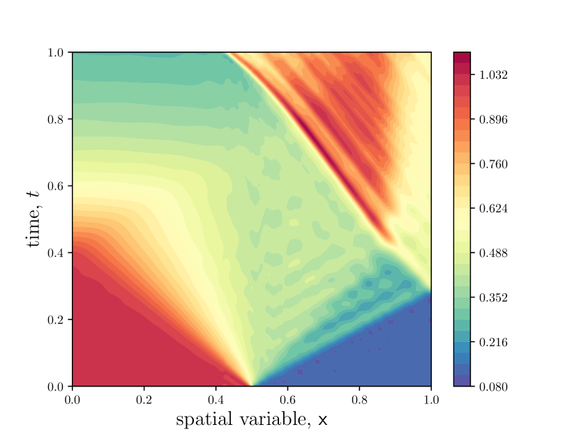
(b) G-ROM

(c) LSPG

(d) WLS: $\Delta T=0.002$

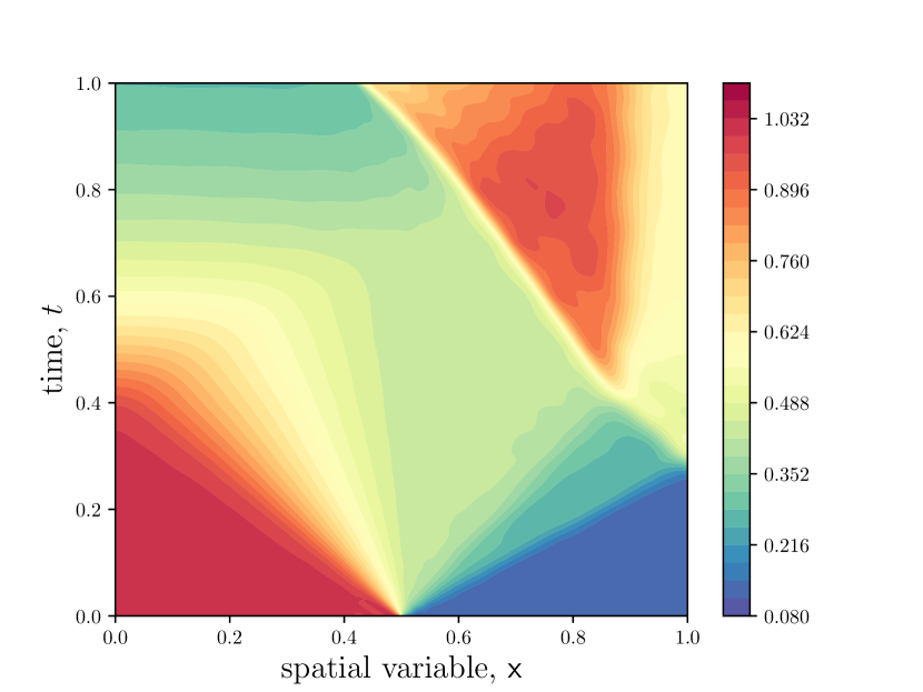
(e) WLS: $\Delta T=0.1$

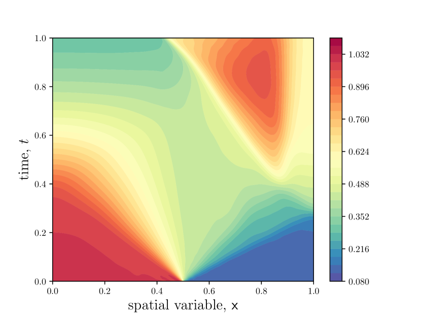
(f) WLS: $\Delta T=1.0$

Figure 5: $\mathsf{x}-t$ diagrams for the density fields as predicted by the FOM, G-ROM, LSPG-ROM, and WLS ROMs.

Next, Figure 6 shows space–time state errors and the objective function (3.3) (i.e., the space–time residual norm) over $t\in[0,1]$ for the various ROMs. Most notably, we observe that increasing the window size over which the residual is minimized does not lead to a monotonic decrease in the space–time error as measured in the $\ell^{2}$-norm (we refer to this as the $\ell^{2}$-error). As expected, increasing the window size does lead to a monotonic decrease in the space–time residual, however. We additionally note that, although the space–time $\ell^{2}$-error of the projected FOM solution is significantly lower than that of the various ROM solutions, the space–time residual norm of the projected FOM solution is higher than all ROMs. Thus, although the projected FOM solution is more accurate in the $\ell^{2}$-norm, it does not satisfy the governing equations as well the ROM solutions.

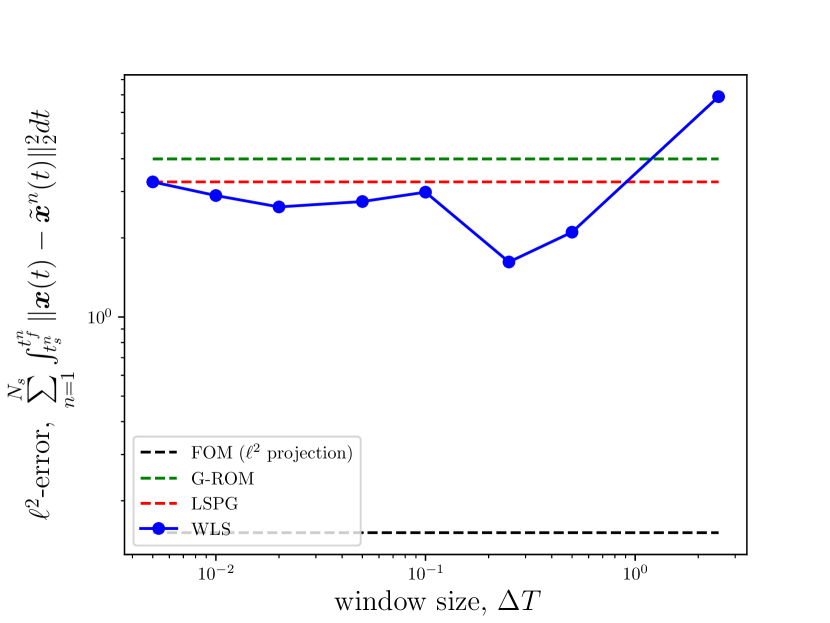
(a) Space–time $\ell^{2}$-error of various ROMs.

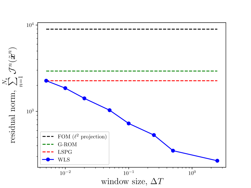
(b) Integrated residual norm of various ROMs.

Figure 6: Integrated performance metrics of the Galerkin, LSPG, and WLS ROMs. Note that the Galerkin and LSPG ROMs do not depend on the window size.

We now examine the comparative performance of the direct and indirect solution techniques for the WLS ROMs using various time discretization techniques. Figure 7 shows the same space–time $\ell^{2}$-errors and residual norms as in Figure 6, but this time results are shown for the various WLS ROMs. In both Figures 9(a) and 9(b), we observe that the WLS method is relatively insensitive to the solution technique (direct vs indirect) and underlying discretization scheme, although some minor differences are observed. In particular, ROMs using the second order explicit AB2 scheme with a time step of $\Delta t=0.0005$ provide similar results to the ROMs using the second-order CN scheme at a time step of $\Delta t=0.002$. All methods display similar dependence on the window size: the optimal $\ell^{2}$-error occurs when the window size is $\Delta T=0.1$, and the residual decreases monotonically as the window size grows.

(a) Integrated $\ell^{2}$-error of the WLS ROMs.

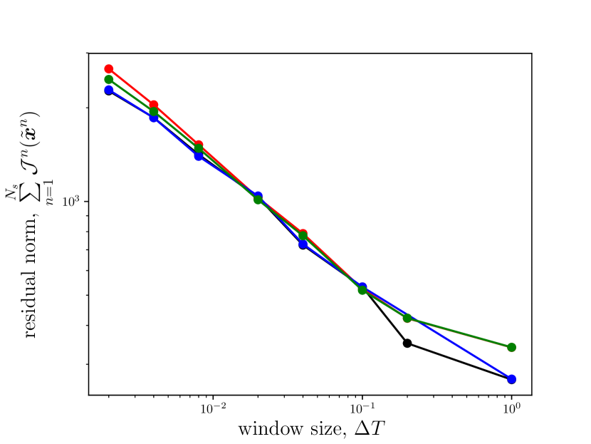
(b) Integrated residual norm of the WLS ROMs.

Figure 7: Integrated performance metrics of various WLS ROMs.

Next, Figure 8 provides the CPU wall-clock times for the various WLS ROMs. We observe that the computational cost of all methods grows as the window size is increased. For indirect methods, this increase in cost is due to the fact that, as the window size grows, more iterations of the FBSM are required for convergence. For direct methods, the increase in cost is due to (1) the cost associated with forming and solving the normal equations at each Gauss–Newton iteration and (2) the increased number of Gauss–Newton iterations required for convergence. We observe the cost of the FBSM method to increase more rapidly than the direct methods. Encouragingly, WLS ROMs based on the CN discretization minimizing the full space–time residual (comprising 500 time instances) only cost approximately one order of magnitude more than the case where the residual is minimized over a single time step (i.e., LSPG). Also of interest is the fact that the direct method utilizing the AB2 time-discretization scheme costs only slightly more per a given window size than the direct method utilizing the CN time discretization. This is despite the fact that AB2 is evolved at a time step of $\Delta t=0.0005$, while CN uses $\Delta t=0.002$; thus AB2 contains 4 times more temporal degrees of freedom than CN. Finally, we emphasize that the results presented here are for standard algorithms (e.g., Gauss–Newton and the FBSM). As mentioned in Remarks 4.2 and 4.3, we expect that the computational cost of both indirect and direct methods can be decreased through the use and/or development of algorithms tailored to the windowed minimization problem.

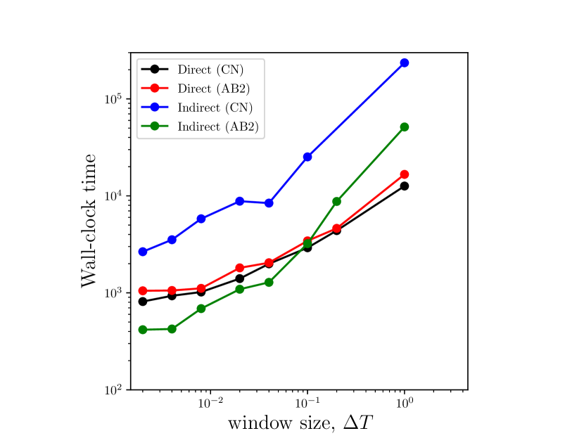
Figure 8: Comparison of wall-clock times of the direct and indirect WLS ROMs as a function of window size.

Finally, we study the impact of the time step on the WLS ROM results. We examine WLS ROMs that use a window size of $\Delta T=0.1$, with time steps $\Delta t=$ $0.001$, $0.002$, $0.005$, $0.01$, $0.05$, $0.1$ (i.e., $100$, $50$, $20$, $10$, $2$, and $1$ time instances per window). We additionally consider LSPG ROMs leveraging the same set of time steps. To assess time step convergence, we compare results to a new full-order model, which is as described in Section 6.1.1 but uses a fine time step of $\Delta t=10^{-4}$. Figure 9 shows the $\ell^{2}$-error and residual norm of the various ROMs. We observe that the $\ell^{2}$-error and residual norm of the WLS ROMs decrease and converge as the time step decreases. This is in direct contrast to the LSPG ROMs, in where the $\ell^{2}$-error and residual norm display a complex dependence on the time step. This result demonstrates that WLS overcomes the time-step dependence inherit to the LSPG approach. Lastly, Figure 10 shows the relative wall-clock times of the WLS ROMs with respect to the LSPG ROMs. It is seen that for all time steps considered, the WLS ROMs are less than 6x the cost of LSPG; this is despite the window sizes comprising up to 100 time instances.

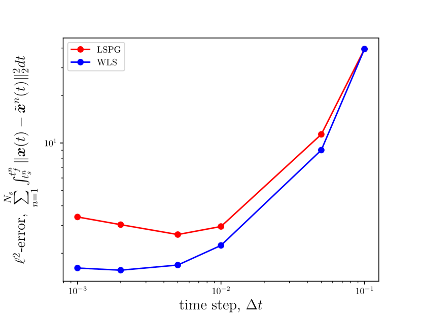
(a) Space–time $\ell^{2}$-error of the WLS ROM.

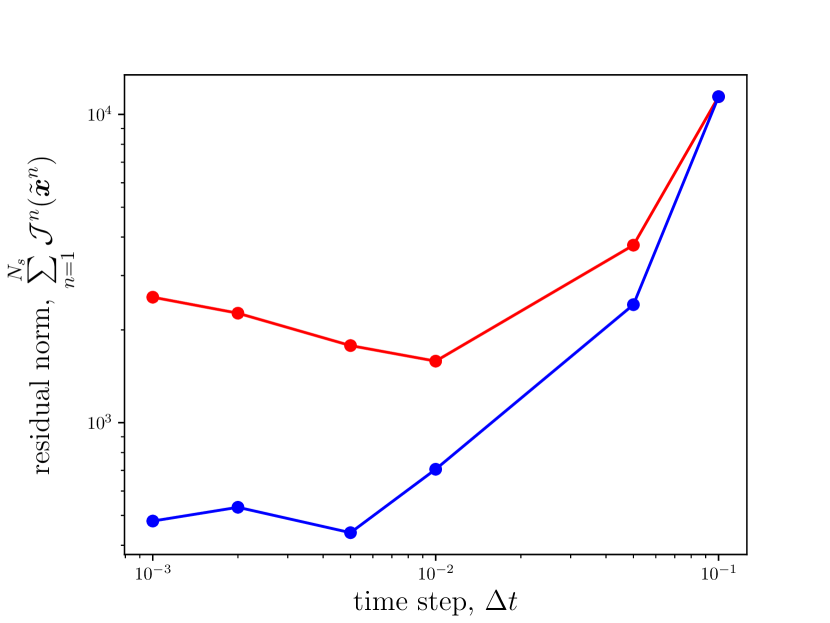
(b) Space–time residual norm of the WLS ROM.

Figure 9: Performance metrics of the Galerkin, LSPG, and WLS ROMs.

Figure 10: Comparison of wall-clock times of the WLS ROMs to LSPG ROMs as a function of the time step. WLS ROMs have a fixed window size of $\Delta T=0.1$.

6.1.4 Summary of numerical results for the Sod shock tube

The key observations from the results of the first numerical example are:

1. Increasing the window size over which the residual is minimized led to more physically relevant solutions. Specifically, we observed that as the window size over which the residual was minimized grew, WLS led to less oscillatory solutions.

2. Increasing the window size over which the residual is minimized does not necessary lead to a lower space–time error as measured by the $\ell^{2}$-norm. We observed that minimizing the residual over an intermediary window size led to the lowest space–time error in the $\ell^{2}$-norm.

3. WLS displays time-step convergence: both the $\ell^{2}$-error and residual norm decreased and displayed time-step convergence as the time step decreased. This is in contrast to LSPG.

4. For all examples considered, in where the windows comprised up to 2000 time instances, WLS with the direct method is between 1x and 10x the cost of the LSPG. The direct method was observed to be slightly more efficient and robust than the indirect method.

6.2 Cavity flow

The next numerical example considers collocated ROMs of a viscous, compressible flow in a two-dimensional cavity. The flow is described by the two-dimensional compressible Navier-Stokes equations,

$$\frac{\partial\mathbf{u}}{\partial t}+\nabla\cdot\big{(}\mathbf{F}(\mathbf{u})-\mathbf{F}_{v}(\mathbf{u},\nabla\mathbf{u})\big{)}=\boldsymbol{0},$$ (6.2)

where $\mathbf{u}:[0,T]\times\Omega\rightarrow\mathbb{R}^{4}$ comprise the density, $\mathsf{x}_{1}$ and $\mathsf{x}_{2}$ momentum, and total energy. The terms $\mathbf{F}$ and $\mathbf{F}_{v}$ are the inviscid and viscous fluxes, respectively. For a two-dimensional flow, the state vector and inviscid fluxes are

$$\mathbf{u}=\begin{Bmatrix}\rho\\ \rho u_{1}\\ \rho u_{2}\\ \rho E\end{Bmatrix},\qquad\mathbf{F}_{1}=\begin{Bmatrix}\rho u_{1}\\ \rho u_{1}^{2}+p\\ \rho u_{1}u_{2}\\ u_{1}(E+p)\end{Bmatrix},\qquad\mathbf{F}_{2}=\begin{Bmatrix}\rho u_{2}\\ \rho u_{1}u_{2}\\ \rho u_{2}^{2}+p\\ u_{2}(E+p)\end{Bmatrix}.$$

The viscous fluxes are given by

$$\qquad\mathbf{F}_{v_{1}}=\begin{Bmatrix}0\\ \tau_{11}\\ \tau_{12}\\ u_{j}\tau_{j1}+c_{p}\frac{\mu}{\text{Pr}}\frac{\partial T}{\partial x_{1}}\end{Bmatrix},\qquad\mathbf{F}_{v_{2}}=\begin{Bmatrix}0\\ \tau_{21}\\ \tau_{22}\\ u_{j}\tau_{j2}+c_{p}\frac{\mu}{\text{Pr}}\frac{\partial T}{\partial x_{2}}\end{Bmatrix},$$

where $\mu\in\mathbb{R}_{+}$ is the dynamic viscosity, $\text{Pr}=0.72$ is the Prandtl number, $T:\Omega\rightarrow\mathbb{R}_{+}$ the temperature, and $c_{p}\in\mathbb{R}_{+}$ the heat capacity ratio. We assume a Newtonian fluid, which leads to a viscous stress tensor of the form

$$\tau_{ij}=2\mu S_{ij},$$

where

$$S_{ij}=\frac{1}{2}\big{(}\frac{\partial u_{i}}{\partial\mathsf{x}_{j}}+\frac{\partial u_{j}}{\partial\mathsf{x}_{i}}\big{)}-\frac{1}{3}\frac{\partial u_{k}}{\partial\mathsf{x}_{i}}\delta_{ij}.$$

We close the Navier–Stokes equations with a constitutive relationship for a calorically perfect gas,

$$p=(\gamma-1)(\rho E-\frac{1}{2}\rho u_{1}^{2}-\frac{1}{2}\rho u_{2}^{2}\big{)},$$

where $\gamma=1.4$ is the heat-capacity ratio.

Figure 11 depicts the domain $\Omega$ and flow conditions. The Reynolds number is defined as $\text{Re}=\rho_{\infty}\|\mathbf{v}_{\infty}\|_{2}L/\mu$ with a characteristic length set at $L=1$ and $\mathbf{v}=[u_{1}\;\;u_{2}]^{T}$, the speed of sound is defined by $a_{\infty}=\sqrt{\gamma p_{\infty}/\rho_{\infty}}$, and $\infty$ subscripts refer to free-stream conditions. We employ free-stream boundary conditions at the inlet, outlet, and top wall of the cavity. We enforce no-slip boundary conditions on the bottom wall of the cavity.

6.2.1 Description of FOM and generation of S-reduction trial subspace

The full-order model comprises a discontinuous-Galerkin discretization. We obtain the discretization by partitioning the domain into $100$ elements in the flow direction and $40$ elements in the wall-normal direction. The discretization represents the solution to third order over each element using tensor product polynomials of order $p=2$, resulting in $36000$ unknowns for each conserved variable. Spatial discretization via the discontinuous Galerkin method yields a dynamical system of the form

$$\frac{d\boldsymbol{x}}{dt}=\mathbf{M}_{\text{DG}}^{-1}\boldsymbol{f}_{\text{DG}}(\boldsymbol{x}),$$

where $\mathbf{M}_{\text{DG}}\in\mathbb{R}^{N\times N}$ is the (block diagonal) DG mass matrix and $\boldsymbol{f}_{\text{DG}}:\mathbb{R}^{N}\rightarrow\mathbb{R}^{N}$ is the DG velocity operator containing surface and volume integrals. By the definition of the FOM (2.1), the dynamical system velocity is $\boldsymbol{f}=\mathbf{M}_{\text{DG}}^{-1}\boldsymbol{f}_{\text{DG}}$. Figure 12 shows the computational mesh. The DG method uses the Rusanov flux at the cell interfaces [57] and uses the first form of Bassi and Rebay [4] for the viscous fluxes. Time integration is performed via a third-order strong stability preserving Runge-Kutta method [32] with a time step of $\Delta t=0.001$.

The reduced-order models leverage POD to construct the S-reduction trial basis and use q-sampling [28] based on snapshots of the FOM velocity to select the sampling points (and as a result the weighting matrix $\mathbf{A}$); we use a constant weighting matrix across all windows, e.g., $\mathbf{A}^{n}\equiv\mathbf{A}$, $n=1,\ldots,N_{w}$. The process used to construct the initial conditions, trial subspaces, and weighting matrices for the ROMs is as follows:

1. Initialize the FOM with uniform free-stream conditions.

2. Evolve the FOM for $t\in[0,400]$.

3. Reset the time coordinate, $0\leftarrow t$, and execute Algorithm 3 with $\mathbf{x}_{\text{ref}}=\boldsymbol{0},N_{\text{skip}}=100$ and $K=\{136,193\}$ over $t\in[0,100]$ to construct two trial subspaces comprising $\approx 95\%$ and $\approx 97\%$ of the snapshot energy, respectively.

4. Execute Algorithm 4 with $N_{\text{skip}}=100$, $n_{s}=129$ to obtain the sampling point matrix of dimension $\mathbf{W}\in\{0,1\}^{1603\times N}$.

Figure 13 shows the resulting sample mesh used in the ROM simulations. To depict the nature of the flow, Figure 14 shows snapshots of the vorticity field generated by the FOM for several time instances used in training.

Basis #	Trial Basis Dimension ($K$)	Energy Criterion	Sample Points ($n_{S}$)
1	$136$	$95.0\%$	$1603$
2	$193$	$97.0\%$	$1603$

Table 1: Summary of the various basis sizes employed in the cavity flow example.

6.2.2 Description of reduced-order models

We consider collocated ROMs based on the Galerkin, least-squares Petrov–Galerkin, and WLS approaches. Details on the implementation of the methods is as follows:

• Galerkin ROM with collocation: We consider a Galerkin ROM with collocation and evolve the ROM in time with the CN time scheme at a time step of $\Delta t=0.1$.

• LSPG ROM with collocation: We consider a collocated LSPG ROM, which is built on top of the FOM discretization using the CN scheme for temporal discretization. We employ a time step of $\Delta t=0.1$. The implementation is the same as previously described.

• WLS ROMs with collocation: We consider WLS ROMs solved via the direct method. The ROMs use the CN time discretization with a time step of $\Delta t=0.1$. The implementation is the same as previously described.

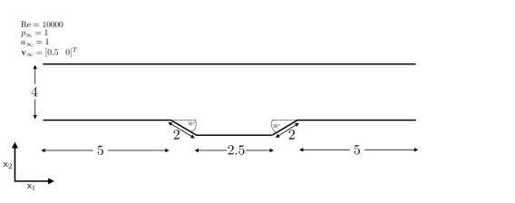
Figure 11: Figure depicting geometry and flow conditions of the cavity flow problem.

Figure 12: Computational mesh employed in cavity flow simulations.

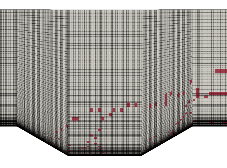
Figure 13: Close up of computational mesh with highlighted collocation cells.

(a) $t=0.0$

(b) $t=4.0$

(c) $t=8.0$

(d) $t=12.0$

(e) $t=16.0$

(f) $t=20.0$

Figure 14: Vorticity snapshots from the FOM simulation at various time instances.

6.2.3 Numerical results

We first assess the performance of WLS ROMs with varying window sizes. To this end, we consider WLS ROMs with uniform window sizes of $\Delta T^{n}\equiv\Delta T=0.2,0.5,1.0,$ and $2.0$, along with the Galerkin and LSPG ROMs. We first consider results for basis #1 as described in Table 1. For all ROMs, we evolve the solution for $t\in[0,100]$. This comprises the same time interval used to construct the trial subspace. First, Figure 15(a) depicts the evolution of the pressure at the bottom wall in the midpoint of the computational domain, while Figure 15(b) depicts the evolution of the normalized $\ell^{2}$-error of the various reduced-order models. Both the collocated Galerkin and LSPG ROMs blow up/fail to converge within the first several time units. The WLS ROM minimizing the residual over a window of size $\Delta T=0.2$ also fails to converge. The WLS ROMs that minimize the residual over window sizes of $\Delta T\geq 0.5$ are seen to all be stable and accurate; the pressure response is well characterized and the normalized state errors are less than $10\%$. The most notable discrepancy between the WLS ROM and FOM solutions is a phase difference.

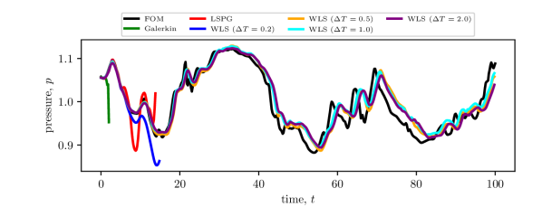
(a) Pressure

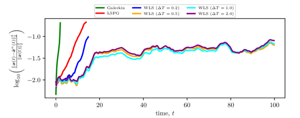
(b) Normalized $\ell^{2}$-error

Figure 15: Comparison of the pressure profiles obtained at the midpoint of the bottom wall (top) and normalized $\ell^{2}$-errors (bottom) of various collocated ROMs to the full-order model solution.

Figure 16 shows the space–time error and objective function of the stable WLS ROMs. We observe that growing the window size over which the residual is minimized leads to a lower space–time residual, but not necessarily a lower $\ell^{2}$-error. This result is consistent with the previous numerical example. Next, Figure 21 shows the wall-clock times of the WLS ROMs for $t\in[0,10]$ as compared to the LSPG ROM. As expected, increasing $\Delta T$ again leads to an increase in computational cost; minimizing the residual over a window comprising 20 time instances yields a 2.5x increase in cost over LSPG.

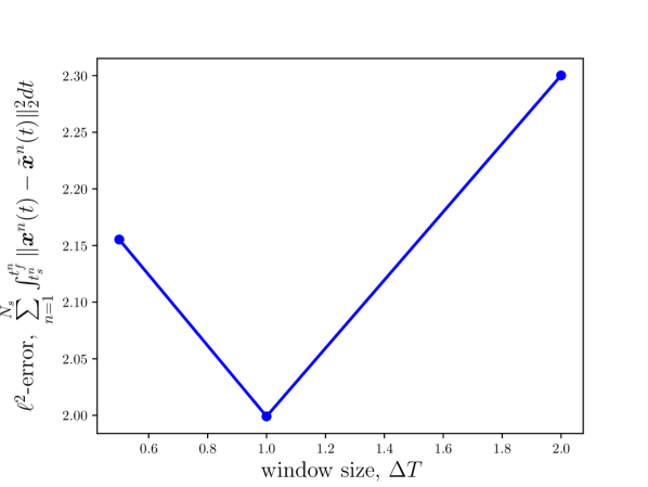
(a) Space–time $\ell^{2}$-error

(b) Objective function

Figure 16: Space–time error (left) and objective function (right) as a function of window size.

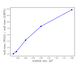
Figure 17: Wall-clock times of WLS ROMs with respect to the LSPG ROM.

Figure 18 shows vorticity fields for the FOM, LSPG ROM, and WLS ROMs with $\Delta T=0.5,1.0$ for the time instance $t=5.0$. LSPG is observed to exhibit artificial oscillations; the Gauss-Newton method fails to converge at $t\approx 16.0$. The WLS ROMs at $\Delta T=0.5,1.0$ are able to capture the important features of the flow, including the points of flow separation at the start and end of the ramp, and remain stable for the entire time interval.

(a) FOM

(b) LSPG

(c) WLS, $\Delta T=0.5$

(d) WLS, $\Delta T=1.0$

Figure 18: Vorticity snapshots from the FOM and ROM simulations at $t=5.0$.

Next, we assess the performance of the various ROMs for basis #2 as described in Table 1, which comprises a richer spatial basis. Figure 19 shows the same pressure and error profiles as Figure 15, but for the enriched basis. The LSPG and Galerkin ROMs blow up faster as compared to Figure 15; LSPG fails to converge around $t\approx 8$ (opposed to $t\approx 16$), while Galerkin blows up almost immediately. The WLS ROMs again yield improved performance: WLS ROMs minimizing the residual over window sizes of $\Delta T\geq 0.5$ are seen to all be stable and accurate; the pressure response is well characterized and the normalized state errors are less than $5\%$. The WLS ROMs employing basis #2 yield more accurate results than WLS ROMs employing basis #1.

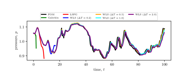
(a) Pressure

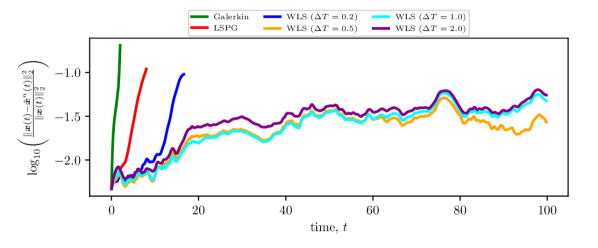
(b) Normalized $\ell^{2}$-error

Figure 19: Comparison of the pressure profiles obtained at the midpoint of the bottom wall (top) and normalized $\ell^{2}$-errors (bottom) of various collocated ROMs to the full-order model solution.

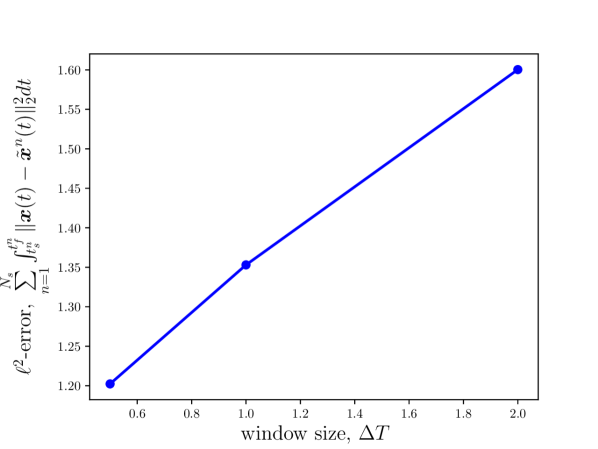
(a) Integrated $\ell^{2}$-error

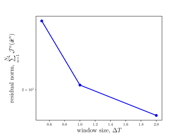
(b) Objective function

Figure 20: Integrated error (left) and objective function (right) as a function of window size.

Finally, Figure 21 shows the wall-clock times for $t\in[0,4]$ of the WLS ROMs as compared to the LSPG ROMs for basis #2. Increasing the window size again leads to an increase in computational cost. Minimizing the residual over a window comprising 20 time instances yields a 3x increase in cost over LSPG.

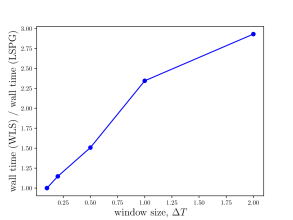
Figure 21: Wall-clock times of WLS ROMs with respect to the LSPG ROM.

7 Conclusions

This paper proposed the windowed least-squares (WLS) approach for model reduction of dynamical systems. The approach sequentially minimizes the time-continuous full-order-model residual within a low-dimensional space–time trial subspace over time windows. The approach was formulated for two types of trial subspaces: one that reduces only the spatial dimension of the full-order model, and one that reduces both the spatial and temporal dimensions of the full-order model. For each type of trial subspace, we outlined two different solution techniques: direct (i.e., discretize then optimize) and indirect (i.e., optimize then discretize). We showed that particular instances of the approach recover Galerkin, least-squares Petrov–Galerkin (LSPG), and space–time LSPG projection. The case of S-reduction trial subspaces is of particular interest in the WLS context: it was shown that indirect methods comprise solving a coupled two-point Hamiltonian boundary value problem. The forward system, which is forced by an auxiliary costate, evolves the (spatial) generalized coordinates of the ROM in time. The backward system, which is forced by the time-continuous FOM residual evaluated about the ROM state, governs the dynamics of the costate.

Numerical experiments of the compressible Euler and Navier–Stokes equations demonstrated the utility in the proposed approach. The first numerical experiment, in where the Sod shock tube was examined, demonstrated that WLS ROMs minimizing the residual over larger time windows yielded solutions with lower space–time residuals. Increasing the window size over which the residual was minimized, however, did not necessarily decrease the solution error in the $\ell^{2}$-norm; we observed this to occur over an intermediary window size. We additionally observed that the WLS approach overcomes the time-discretization sensitivity that LSPG is subject to. The second numerical experiment, which examined collocated ROMs of a compressible cavity flow, demonstrated the utility of the WLS formulation on a more complex flow. In this experiment, WLS ROMs yielded predictions with relative errors less than $5-10\%$, while the Galerkin and LSPG ROMs failed to converge/blew up. Increasing the window size over which the residual was minimized again led to a lower space–time residual, but not necessarily a lower error in the $\ell^{2}$-norm.

The principal challenge encountered in the WLS formulation is the computational cost: increasing the window size over which the residual is minimized leads to a higher computational cost. In the context of the direct solution approach, this increased cost is due to the increased expense of forming and solving the least-squares problem associated with larger window sizes. In the context of indirect methods, this increased cost is a result of the increased number of iterations of the forward backward sweep method. While numerical experiments demonstrated that the increase in computational cost is mild, future work will target the development of new solution techniques tailored for the WLS approach.

8 Acknowledgments

The authors thank Yukiko Shimizu and Patrick Blonigan for numerous conversations from which this work benefited. E. Parish acknowledges an appointment to the Sandia National Laboratories’ John von Neumann Postdoctoral Research Fellowship in Computational Science. This work was partially sponsored by Sandia’s Advanced Simulation and Computing (ASC) Verification and Validation (V&V) Project/Task #103723/05.30.02. This paper describes objective technical results and analysis. Any subjective views or opinions that might be expressed in the paper do not necessarily represent the views of the U.S. Department of Energy or the United States Government. Sandia National Laboratories is a multimission laboratory managed and operated by National Technology and Engineering Solutions of Sandia, LLC., a wholly owned subsidiary of Honeywell International, Inc., for the U.S.  Department of Energy’s National Nuclear Security Administration under contract DE-NA-0003525.

Appendix A Proper orthogonal decomposition

Algorithm 3 presents the algorithm for computing the trial basis via proper orthogonal decomposition.

Input: Number of time-steps between snapshots $N_{\text{skip}}$; intercept $\mathbf{x}_{\text{ref}}$; basis dimension $K$ ;

Output: POD Basis $\mathbf{V}\in\mathbb{V}_{K}(\mathbb{R}^{N})$ ;

Steps:

1. Solve FOM O$\Delta$E and collect solutions into snapshot matrix

   $$\mathbf{S}(N_{\text{skip}})\vcentcolon=\begin{bmatrix}{\mathbf{x}}^{0}-\mathbf{x}_{\text{ref}}^{n}&{\mathbf{x}}^{N_{\text{skip}}}-\mathbf{x}_{\text{ref}}^{n}&\cdots&{\mathbf{x}}^{\text{floor}(N_{t}/N_{\text{skip}})N_{\text{skip}}}-\mathbf{x}_{\text{ref}}^{n}\end{bmatrix}$$

2. Compute the thin singular value decomposition,

   $$\mathbf{S}(N_{\text{skip}})=\mathbf{U\Sigma Z}^{T},$$

   where $\mathbf{U}\equiv\begin{bmatrix}\mathbf{u}_{1}&\cdots&\mathbf{u}_{\text{floor}(N_{t}/N_{\text{skip}})}\end{bmatrix}$

3. Truncate left singular vectors and to form the basis, $\mathbf{V}\equiv\begin{bmatrix}\mathbf{u}_{1}&\cdots&\mathbf{u}_{K}\end{bmatrix}$

Algorithm 3 Algorithm for generating POD Basis.

Appendix B Selection of sampling points

To construct the sampling point matrix used for hyper-reduction in the second numerical experiment, we employ q-sampling [28] and the sample mesh concept [21]. Algorithm 4 outlines the steps used in the second numerical experiment to compute the sampling points.

Input: Number of time-steps between snapshots $N_{\text{skip}}$, number of primal sampling points, $n_{s}$ ;

Output: Weighting matrix $\mathbf{A}\equiv[\mathbf{W}]^{T}\mathbf{W}\in\{0,1\}^{N\times N}$ ;

Steps:

1. Solve FOM O$\Delta$E and collect velocity snapshots

   $$\mathbf{F}(N_{\text{skip}})\vcentcolon=\begin{bmatrix}\boldsymbol{f}({\mathbf{x}}^{0})&\boldsymbol{f}({\mathbf{x}}^{N_{\text{skip}}})&\cdots&\boldsymbol{f}({\mathbf{x}}^{\text{floor}(N_{t}/N_{\text{skip}})N_{\text{skip}}})\end{bmatrix}$$

2. Compute the thin singular value decomposition,

   $$\mathbf{F}(N_{\text{skip}})=\mathbf{U\Sigma Z}^{T},$$

   where $\mathbf{U}\equiv\begin{bmatrix}\mathbf{u}_{1}&\cdots&\mathbf{u}_{\text{floor}(N_{t}/N_{\text{skip}})}\end{bmatrix}$

3. Compute the QR factorization of $\mathbf{U}^{T}$ with column pivoting,

   $$\mathbf{U}^{T}\mathbf{P}^{*}=\mathbf{QR}$$

   with $\mathbf{P}^{*}\equiv\begin{bmatrix}\mathbf{p}_{1}&\cdots&\mathbf{p}_{\text{floor}(N_{t}/N_{\text{skip}})}\end{bmatrix}$, $\mathbf{p}_{i}\in\{0,1\}^{N}$.

4. Select the first $n_{s}$ columns of $\mathbf{P}^{*}$ to form the sampling point matrix $[\mathbf{W}]^{T}\in\{0,1\}^{N\times n_{s}}$.

5. Augment the sampling point matrix, $\mathbf{W}$, with additional columns such that all unknowns are computed at the mesh cells selected by Step 3. For the second numerical experiment, these additional unknowns correspond to each conserved variable and quadrature point in the selected cells.

Algorithm 4 Algorithm for generating the sampling matrix through q-sampling.

Appendix C Derivation of the Euler–Lagrange equations

This section details the derivation of the Euler–Lagrange equations. To this end, we consider the generic functional of the form,

$$\mathcal{J}:(\boldsymbol{y},{\boldsymbol{v}})\mapsto\int_{a}^{b}\mathcal{I}(\boldsymbol{y}(t),{\boldsymbol{v}}(t),t)dt,$$ (C.1)

where $\mathcal{I}:\mathbb{R}^{M}\times\mathbb{R}^{M}\times[a,b]\rightarrow\mathbb{R}_{+}$ (for arbitrary $M$) with $\mathcal{I}:(\mathbf{y},\mathbf{{v}},\tau)\mapsto\mathcal{I}(\mathbf{y},\mathbf{{v}},\tau)$. We now introduce the function $\boldsymbol{z}:[a,b]\rightarrow\mathbb{R}^{M}$ with $\boldsymbol{z}:\tau\mapsto\boldsymbol{z}(\tau)$ along with $\dot{\boldsymbol{z}}\equiv d\boldsymbol{z}/d\tau$. We define this function to be a stationary point of (C.1) (with $\boldsymbol{z}$ being the first argument and $\dot{\boldsymbol{z}}$ being the second argument) subject to the boundary condition $\boldsymbol{z}(a)=\boldsymbol{z}_{a}$. We additionally introduce an arbitrary function $\boldsymbol{\eta}:[a,b]\rightarrow\mathbb{R}^{M}$ with the boundary condition $\boldsymbol{\eta}(a)=\boldsymbol{0}$ and define a variation from the stationary point by

$$\overline{\boldsymbol{z}} :(\tau,\delta)\mapsto\boldsymbol{z}(\tau)+\delta\boldsymbol{\eta}(\tau),$$

$$:[a,b]\times\mathbb{R}\rightarrow\mathbb{R}^{M}.$$

We note that $\overline{\boldsymbol{z}}$ satisfies the same boundary condition $\boldsymbol{z}$ since $\boldsymbol{\eta}(a)=\boldsymbol{0}$. We define a new function that is equivalent to the function (C.1) evaluated at $\overline{\boldsymbol{z}}$ in the first argument and $\dot{\overline{\boldsymbol{z}}}\equiv d\overline{\boldsymbol{z}}/d\tau$ in the second argument,

$$\mathcal{J}_{\delta}:\delta\mapsto\int_{a}^{b}\mathcal{I}(\overline{\boldsymbol{z}}(t,\delta),\dot{\overline{\boldsymbol{z}}}(t,\delta),t)dt.$$

The objective is to now find $\overline{\boldsymbol{z}}$ that makes $\mathcal{J}_{\delta}$ stationary. This can be done by differentiating with respect to $\delta$ and setting the result to zero, i.e.,

$$\frac{d}{d\delta}\big{(}\mathcal{J}_{\delta}\big{)}=0.$$ (C.2)

Using the chain rule,

$$\frac{d}{d\delta}\big{(}\mathcal{J}_{\delta}\big{)}(\epsilon)=\int_{a}^{b}\bigg{[}\frac{\partial\mathcal{I}}{\partial\mathbf{y}}\big{(}\overline{\boldsymbol{z}}(t,\epsilon),\dot{\overline{\boldsymbol{z}}}(t,\epsilon),t\big{)}\frac{\partial\overline{\boldsymbol{z}}}{\partial\delta}(t,\epsilon)+\frac{\partial\mathcal{I}}{\partial\mathbf{{v}}}\big{(}\overline{\boldsymbol{z}}(t,\epsilon),\dot{\overline{\boldsymbol{z}}}(t,\epsilon),t\big{)}\frac{\partial\dot{\overline{\boldsymbol{z}}}}{\partial\delta}(t,\epsilon)\bigg{]}dt.$$

Noting that

$$\frac{\partial\overline{\boldsymbol{z}}}{\partial\delta}(t,\cdot)=\boldsymbol{\eta}(t),\qquad\frac{\partial\dot{\overline{\boldsymbol{z}}}}{\partial\delta}(t,\cdot)=\dot{\boldsymbol{\eta}}(t),$$

where $\dot{\boldsymbol{\eta}}\equiv d\boldsymbol{\eta}/d\tau$, we have

$$\frac{d}{d\delta}\big{(}\mathcal{J}_{\delta}\big{)}(\epsilon)=\int_{a}^{b}\bigg{[}\frac{\partial\mathcal{I}}{\partial\mathbf{y}}\big{(}\overline{\boldsymbol{z}}(t,\epsilon),\dot{\overline{\boldsymbol{z}}}(t,\epsilon),t\big{)}\boldsymbol{\eta}(t)+\frac{\partial\mathcal{I}}{\partial\mathbf{{v}}}\big{(}\overline{\boldsymbol{z}}(t,\epsilon),\dot{\overline{\boldsymbol{z}}}(t,\epsilon),t\big{)}\dot{\boldsymbol{\eta}}(t)\bigg{]}dt.$$

We integrate the second term by parts,

$$\frac{d}{d\delta}\big{(}\mathcal{J}_{\delta}\big{)}(\epsilon)=\int_{a}^{b}\bigg{[}\frac{\partial\mathcal{I}}{\partial\mathbf{y}}\big{(}\overline{\boldsymbol{z}}(t,\epsilon),\dot{\overline{\boldsymbol{z}}}(t,\epsilon),t\big{)}\boldsymbol{\eta}(t)-\frac{d}{dt}\bigg{(}\frac{\partial\mathcal{I}}{\partial\mathbf{{v}}}\big{(}\overline{\boldsymbol{z}}(t,\epsilon),\dot{\overline{\boldsymbol{z}}}(t,\epsilon),t\big{)}\bigg{)}\boldsymbol{\eta}(t)\bigg{]}dt+\\ \frac{\partial\mathcal{I}}{\partial\mathbf{{v}}}\big{(}\overline{\boldsymbol{z}}(b,\epsilon),\dot{\overline{\boldsymbol{z}}}(b,\epsilon),b\big{)}\boldsymbol{\eta}(b),$$ (C.3)

where we have used $\boldsymbol{\eta}(a)=\boldsymbol{0}$. Substituting Eq. (C.3) in the stationarity condition (C.2) yields

$$\int_{a}^{b}\bigg{[}\frac{\partial\mathcal{I}}{\partial\mathbf{y}}\big{(}\overline{\boldsymbol{z}}(t,\epsilon),\dot{\overline{\boldsymbol{z}}}(t,\epsilon),t\big{)}\boldsymbol{\eta}(t)-\frac{d}{dt}\bigg{(}\frac{\partial\mathcal{I}}{\partial\mathbf{{v}}}\big{(}\overline{\boldsymbol{z}}(t,\epsilon),\dot{\overline{\boldsymbol{z}}}(t,\epsilon),t\big{)}\bigg{)}\boldsymbol{\eta}(t)\bigg{]}dt+\frac{\partial\mathcal{I}}{\partial\mathbf{{v}}}\big{(}\overline{\boldsymbol{z}}(b,\epsilon),\dot{\overline{\boldsymbol{z}}}(b,\epsilon),b\big{)}\boldsymbol{\eta}(b)=0.$$ (C.4)

By construction, $\boldsymbol{z}(\cdot)\equiv\overline{\boldsymbol{z}}(\cdot;0)$ and $\dot{\boldsymbol{z}}(\cdot)\equiv\dot{\overline{\boldsymbol{z}}}(\cdot;0)$, comprise a stationary point; thus, setting $\epsilon=0$ in Eq. (C.4) yields

$$\int_{a}^{b}\bigg{[}\frac{\partial\mathcal{I}}{\partial\mathbf{y}}\big{(}\boldsymbol{z}(t),\dot{\boldsymbol{z}}(t),t\big{)}\boldsymbol{\eta}(t)-\frac{d}{dt}\bigg{(}\frac{\partial\mathcal{I}}{\partial\mathbf{{v}}}\big{(}\boldsymbol{z}(t),\dot{\boldsymbol{z}}(t),t\big{)}\bigg{)}\boldsymbol{\eta}(t)\bigg{]}dt+\frac{\partial\mathcal{I}}{\partial\mathbf{{v}}}\big{(}\boldsymbol{z}(b),\dot{\boldsymbol{z}}(b),b\big{)}\boldsymbol{\eta}(b)=0.$$ (C.5)

As $\boldsymbol{\eta}$ is an arbitrary function, this equality requires

$$\begin{split}\bigg{[}&\frac{\partial\mathcal{I}}{\partial\mathbf{y}}\big{(}\boldsymbol{z}(t),\dot{\boldsymbol{z}}(t),t\big{)}\bigg{]}^{T}-\bigg{[}\frac{d}{dt}\bigg{(}\frac{\partial\mathcal{I}}{\partial\mathbf{{v}}}\big{(}\boldsymbol{z}(t),\dot{\boldsymbol{z}}(t),t\big{)}\bigg{)}\bigg{]}^{T}=\boldsymbol{0},\\ &\boldsymbol{z}(a)=\boldsymbol{z}_{a},\hskip 46.97505pt\bigg{[}\frac{\partial\mathcal{I}}{\partial\mathbf{{v}}}\big{(}\boldsymbol{z}(b),\dot{\boldsymbol{z}}(b),b\big{)}\bigg{]}^{T}=\boldsymbol{0}.\end{split}$$ (C.6)

Equation (C.6) is known as the Euler–Lagrange equation. It states that, for ($\boldsymbol{z}$,$\dot{\boldsymbol{z}}$) to define a stationary point of $\mathcal{J}$, then they must satisfy (C.6). It is emphasized that (C.6) is a necessary condition on ($\boldsymbol{z},\dot{\boldsymbol{z}}$) to make $\mathcal{J}$ stationary, but it is not a sufficient condition. It is additionally noted that (C.6) provides a stationary point of $\mathcal{J}$, but the resulting stationary point could be a local minima, local maxima, or saddle point.

Appendix D Evaluation of gradients in the Euler–Lagrange equations for WLS with S-reduction trial subspaces

We now derive the specific form of the Euler–Lagrange equations for the WLS formulation with S-reduction trial subspaces. Without loss of generality, we present the derivation for a single window $t\in[0,T]$ with a constant basis $\mathbf{V}$ and weighting matrix $\mathbf{A}$. To obtain the specific form of the Euler–Lagrange equations for the WLS formulation, we need to evaluate the gradients in (C.6) for the integrand

$$\mathcal{I} \vcentcolon(\hat{\mathbf{y}},\hat{\mathbf{v}},\tau)\mapsto\frac{1}{2}\big{[}\mathbf{V}\hat{\mathbf{v}}-\boldsymbol{f}(\mathbf{V}\hat{\mathbf{y}}+\mathbf{x}_{\text{ref}},\tau)\big{]}^{T}\mathbf{A}\big{[}\mathbf{V}\hat{\mathbf{v}}-\boldsymbol{f}(\mathbf{V}\hat{\mathbf{y}}+\mathbf{x}_{\text{ref}},\tau)\big{]},$$

$$\vcentcolon\mathbb{R}^{K}\times\mathbb{R}^{K}\times[0,T]\rightarrow\mathbb{R}.$$

To evaluate the gradients, we first expand $\mathcal{I}$:

$$\mathcal{I}(\hat{\mathbf{y}},\hat{\mathbf{v}},\tau) =\frac{1}{2}\big{[}\mathbf{V}\hat{\mathbf{v}}-\boldsymbol{f}(\mathbf{V}\hat{\mathbf{y}}+\mathbf{x}_{\text{ref}},\tau)\big{]}^{T}\mathbf{A}\big{[}\mathbf{V}\hat{\mathbf{v}}-\boldsymbol{f}(\mathbf{V}\hat{\mathbf{y}}+\mathbf{x}_{\text{ref}},\tau)\big{]}$$

$$=\frac{1}{2}\big{[}\mathbf{V}\hat{\mathbf{v}}\big{]}^{T}\mathbf{A}\big{[}\mathbf{V}\hat{\mathbf{v}}\big{]}-\frac{1}{2}\big{[}\boldsymbol{f}(\mathbf{V}\hat{\mathbf{y}}+\mathbf{x}_{\text{ref}},\tau)\big{]}^{T}\mathbf{A}\big{[}\mathbf{V}\hat{\mathbf{v}}\big{]}-\frac{1}{2}\big{[}\mathbf{V}\hat{\mathbf{v}}\big{]}^{T}\mathbf{A}\big{[}\boldsymbol{f}(\mathbf{V}\hat{\mathbf{y}}+\mathbf{x}_{\text{ref}},\tau)\big{]}$$

$$+\frac{1}{2}\big{[}\boldsymbol{f}(\mathbf{V}\hat{\mathbf{y}}+\mathbf{x}_{\text{ref}},\tau)\big{]}^{T}\mathbf{A}\big{[}\boldsymbol{f}(\mathbf{V}\hat{\mathbf{y}}+\mathbf{x}_{\text{ref}},\tau)\big{]}.$$

Since $\mathbf{A}$ is symmetric,

$$\mathcal{I}(\hat{\mathbf{y}},\hat{\mathbf{v}},\tau)=\frac{1}{2}\big{[}\mathbf{V}\hat{\mathbf{v}}\big{]}^{T}\mathbf{A}\big{[}\mathbf{V}\hat{\mathbf{v}}\big{]}-\big{[}\mathbf{V}\hat{\mathbf{v}}\big{]}^{T}\mathbf{A}\big{[}\boldsymbol{f}(\mathbf{V}\hat{\mathbf{y}}+\mathbf{x}_{\text{ref}},\tau)\big{]}+\frac{1}{2}\big{[}\boldsymbol{f}(\mathbf{V}\hat{\mathbf{y}}+\mathbf{x}_{\text{ref}},\tau)\big{]}^{T}\mathbf{A}\big{[}\boldsymbol{f}(\mathbf{V}\hat{\mathbf{y}}+\mathbf{x}_{\text{ref}},\tau)\big{]}.$$ (D.1)

For notational purposes, we write the above as,

$$\mathcal{I}(\hat{\mathbf{y}},\hat{\mathbf{v}},\tau)=\mathcal{I}_{1}(\hat{\mathbf{y}},\hat{\mathbf{v}},\tau)+\mathcal{I}_{2}(\hat{\mathbf{y}},\hat{\mathbf{v}},\tau)+\mathcal{I}_{3}(\hat{\mathbf{y}},\hat{\mathbf{v}},\tau),$$

where

$$\mathcal{I}_{1}(\hat{\mathbf{y}},\hat{\mathbf{v}},\tau)=\frac{1}{2}\big{[}\mathbf{V}\hat{\mathbf{v}}\big{]}^{T}\mathbf{A}\big{[}\mathbf{V}\hat{\mathbf{v}}\big{]},$$

$$\mathcal{I}_{2}(\hat{\mathbf{y}},\hat{\mathbf{v}},\tau)=-\big{[}\mathbf{V}\hat{\mathbf{v}}\big{]}^{T}\mathbf{A}\big{[}\boldsymbol{f}(\mathbf{V}\hat{\mathbf{y}}+\mathbf{x}_{\text{ref}},\tau)\big{]},$$

$$\mathcal{I}_{3}(\hat{\mathbf{y}},\hat{\mathbf{v}},\tau)=\frac{1}{2}\big{[}\boldsymbol{f}(\mathbf{V}\hat{\mathbf{y}}+\mathbf{x}_{\text{ref}},\tau)\big{]}^{T}\mathbf{A}\big{[}\boldsymbol{f}(\mathbf{V}\hat{\mathbf{y}}+\mathbf{x}_{\text{ref}},\tau)\big{]}.$$

Constructing the Euler–Lagrange equations for this functional $\mathcal{I}$ requires evaluating the derivatives $\frac{\partial\mathcal{I}}{\partial\hat{\mathbf{y}}}$ and $\frac{\partial\mathcal{I}}{\partial\hat{\mathbf{v}}}$. We start by evaluating $\frac{\partial\mathcal{I}}{\partial\hat{\mathbf{y}}}$ and go term by term.

Starting with $\mathcal{I}_{1}(\hat{\mathbf{y}},\hat{\mathbf{v}})$, we see,

$$\frac{\partial\mathcal{I}_{1}}{\partial\hat{\mathbf{y}}}=\boldsymbol{0},$$

where it is noted that $\mathcal{I}_{1}$ only depends on $\hat{\mathbf{v}}$. Working with the second term:

$$\frac{\partial\mathcal{I}_{2}}{\partial\hat{\mathbf{y}}} =-\frac{\partial}{\partial\hat{\mathbf{y}}}\bigg{(}\big{[}\mathbf{V}\hat{\mathbf{v}}\big{]}^{T}\mathbf{A}\big{[}\boldsymbol{f}(\mathbf{V}\hat{\mathbf{y}}+\mathbf{x}_{\text{ref}},\tau)\big{]}\bigg{)}$$

$$=-\big{[}\mathbf{V}\hat{\mathbf{v}}\big{]}^{T}\mathbf{A}\frac{\partial}{\partial\hat{\mathbf{y}}}\bigg{(}\big{[}\boldsymbol{f}(\mathbf{V}\hat{\mathbf{y}}+\mathbf{x}_{\text{ref}},\tau)\big{]}\bigg{)}$$

$$=-\big{[}\mathbf{V}\hat{\mathbf{v}}\big{]}^{T}\mathbf{A}\frac{\partial\boldsymbol{f}}{\partial\mathbf{y}}\frac{\partial\mathbf{y}}{\partial\hat{\mathbf{y}}}$$

$$=-\big{[}\mathbf{V}\hat{\mathbf{v}}\big{]}^{T}\mathbf{A}\frac{\partial\boldsymbol{f}}{\partial\mathbf{y}}\mathbf{V}$$

$$=-[\hat{\mathbf{v}}]^{T}\mathbf{V}^{T}\mathbf{A}\frac{\partial\boldsymbol{f}}{\partial\mathbf{y}}\mathbf{V},$$

where we have suppressed the arguments of the Jacobian for simplicity; e.g., formally

$$\frac{\partial\boldsymbol{f}}{\partial\mathbf{y}}:(\mathbf{w},\tau)\mapsto\frac{\partial\boldsymbol{f}}{\partial\mathbf{y}}(\mathbf{w},\tau).$$

For $\mathcal{I}_{3}$,

$$\frac{\partial\mathcal{I}_{3}}{\partial\hat{\mathbf{y}}} =\frac{1}{2}\frac{\partial}{\partial\hat{\mathbf{y}}}\bigg{(}\big{[}\boldsymbol{f}(\mathbf{V}\hat{\mathbf{y}}+\mathbf{x}_{\text{ref}},\tau)\big{]}^{T}\mathbf{A}\big{[}\boldsymbol{f}(\mathbf{V}\hat{\mathbf{y}}+\mathbf{x}_{\text{ref}},\tau)\big{]}\bigg{)}$$ (D.2)

$$=[\boldsymbol{f}(\mathbf{V}\hat{\mathbf{y}}+\mathbf{x}_{\text{ref}},\tau)]^{T}\mathbf{A}\frac{\partial\boldsymbol{f}}{\partial\mathbf{y}}\frac{\partial\mathbf{y}}{\partial\hat{\mathbf{y}}}$$ (D.3)

$$=[\boldsymbol{f}(\mathbf{V}\hat{\mathbf{y}}+\mathbf{x}_{\text{ref}},\tau)]^{T}\mathbf{A}\frac{\partial\boldsymbol{f}}{\partial\mathbf{y}}\mathbf{V}.$$ (D.4)

This gives the final expression,

$$\frac{\partial\mathcal{I}}{\partial\boldsymbol{\hat{\mathbf{y}}}}=-\big{[}\mathbf{V}\hat{\mathbf{v}}\big{]}^{T}\mathbf{A}\frac{\partial\boldsymbol{f}}{\partial\mathbf{y}}\mathbf{V}+[\boldsymbol{f}(\mathbf{V}\hat{\mathbf{y}}+\mathbf{x}_{\text{ref}},\tau)]^{T}\mathbf{A}\frac{\partial\boldsymbol{f}}{\partial\mathbf{y}}\mathbf{V}.$$

We now evaluate $\frac{\partial\mathcal{I}}{\partial\hat{\mathbf{v}}}$ and again go term by term. Starting with $\mathcal{I}_{1}$,

$$\frac{\partial\mathcal{I}_{1}}{\partial\hat{\mathbf{v}}} =\frac{1}{2}\frac{\partial}{\partial\hat{\mathbf{v}}}\bigg{(}\big{[}\mathbf{V}\hat{\mathbf{v}}\big{]}\mathbf{A}\big{[}\mathbf{V}\hat{\mathbf{v}}\big{]}\bigg{)}$$

$$=[\hat{\mathbf{v}}]^{T}\mathbf{V}^{T}\mathbf{A}\mathbf{V}.$$

Now working with the second term:

$$\frac{\partial\mathcal{I}_{2}}{\partial\hat{\mathbf{v}}} =\frac{\partial}{\partial\hat{\mathbf{v}}}\bigg{(}\big{[}\mathbf{V}\hat{\mathbf{v}}\big{]}^{T}\mathbf{A}\big{[}\boldsymbol{f}(\mathbf{V}\hat{\mathbf{y}}+\mathbf{x}_{\text{ref}},\tau)\big{]}\bigg{)}$$

$$=\frac{\partial}{\partial\hat{\mathbf{v}}}\bigg{(}[\hat{\mathbf{v}}]^{T}\bigg{)}\mathbf{V}^{T}\mathbf{A}\big{[}\boldsymbol{f}(\mathbf{V}\hat{\mathbf{y}}+\mathbf{x}_{\text{ref}},\tau)\big{]}$$

$$=\bigg{[}\mathbf{V}^{T}\mathbf{A}\boldsymbol{f}(\mathbf{V}\hat{\mathbf{y}}+\mathbf{x}_{\text{ref}},\tau)\bigg{]}^{T}$$

$$=[\boldsymbol{f}(\mathbf{V}\hat{\mathbf{y}}+\mathbf{x}_{\text{ref}},\tau)]^{T}\mathbf{A}\mathbf{V}.$$

Finally, for the last term,

$$\frac{\partial\mathcal{I}_{3}}{\partial\hat{\mathbf{v}}} =\boldsymbol{0},$$

where it is noted that $\mathcal{I}_{3}$ only depends on $\hat{\mathbf{y}}$. We thus have,

$$\frac{\partial\mathcal{I}}{\partial\hat{\mathbf{v}}}=[\hat{\mathbf{v}}]^{T}\mathbf{V}^{T}\mathbf{A}\mathbf{V}-[\boldsymbol{f}(\mathbf{V}\hat{\mathbf{y}}+\mathbf{x}_{\text{ref}},\tau)]^{T}\mathbf{A}\mathbf{V}.$$

Combining all terms and evaluating at $(\hat{\boldsymbol{x}}(t),\dot{\hat{\boldsymbol{x}}}(t),t)$,

$$\frac{\partial\mathcal{I}}{\partial\hat{\mathbf{y}}}(\hat{\boldsymbol{x}}(t),\dot{\hat{\boldsymbol{x}}}(t),t)-\frac{d}{dt}\bigg{[}\frac{\partial\mathcal{I}}{\partial\hat{\mathbf{v}}}(\hat{\boldsymbol{x}}(t),\dot{\hat{\boldsymbol{x}}}(t),t)\bigg{]}=-\big{[}\mathbf{V}\dot{\hat{\boldsymbol{x}}}(t)\big{]}^{T}\mathbf{A}\big{[}\frac{\partial\boldsymbol{f}}{\partial\mathbf{y}}(\mathbf{V}\hat{\boldsymbol{x}}(t)+\mathbf{x}_{\text{ref}},t)\big{]}\mathbf{V}+\\ [\boldsymbol{f}(\mathbf{V}\hat{\boldsymbol{x}}(t)+\mathbf{x}_{\text{ref}},t)]^{T}\mathbf{A}\big{[}\frac{\partial\boldsymbol{f}}{\partial\mathbf{y}}(\mathbf{V}\hat{\boldsymbol{x}}(t)+\mathbf{x}_{\text{ref}},t)\big{]}\mathbf{V}-\frac{d}{dt}\bigg{[}[\dot{\hat{\boldsymbol{x}}}(t)]^{T}\mathbf{V}^{T}\mathbf{A}\mathbf{V}-[\boldsymbol{f}(\mathbf{V}\hat{\boldsymbol{x}}(t)+\mathbf{x}_{\text{ref}},t)]^{T}\mathbf{A}\mathbf{V}\bigg{]}=\boldsymbol{0}.$$

To put this in a more recognizable form, we can pull out the common factor in the first two terms,

$$-\bigg{(}\big{[}\mathbf{V}\dot{\hat{\boldsymbol{x}}}(t)\big{]}^{T}-[\boldsymbol{f}(\mathbf{V}\hat{\boldsymbol{x}}(t)+\mathbf{x}_{\text{ref}},t)]^{T}\bigg{)}\mathbf{A}\frac{\partial\boldsymbol{f}}{\partial\mathbf{y}}(\mathbf{V}\hat{\boldsymbol{x}}(t)+\mathbf{x}_{\text{ref}},t)\mathbf{V}-\\ \frac{d}{dt}\bigg{[}[\dot{\hat{\boldsymbol{x}}}(t)]^{T}\mathbf{V}^{T}\mathbf{A}\mathbf{V}-[\boldsymbol{f}(\mathbf{V}\hat{\boldsymbol{x}}(t)+\mathbf{x}_{\text{ref}},t)]^{T}\mathbf{A}\mathbf{V}\bigg{]}=\boldsymbol{0}.$$

Taking the transpose to put into the common column major format,

$$-\mathbf{V}^{T}\big{[}\frac{\partial\boldsymbol{f}}{\partial\mathbf{y}}(\mathbf{V}\hat{\boldsymbol{x}}(t)+\mathbf{x}_{\text{ref}},t)\big{]}^{T}\mathbf{A}\bigg{(}\big{[}\mathbf{V}\dot{\hat{\boldsymbol{x}}}(t)\big{]}-\boldsymbol{f}(\mathbf{V}\hat{\boldsymbol{x}}(t)+\mathbf{x}_{\text{ref}},t)\bigg{)}-\frac{d}{dt}\bigg{[}\mathbf{V}^{T}\mathbf{A}\mathbf{V}\dot{\hat{\boldsymbol{x}}}(t)-\mathbf{V}^{T}\mathbf{A}\boldsymbol{f}(\mathbf{V}\hat{\boldsymbol{x}}(t)+\mathbf{x}_{\text{ref}},t)\bigg{]}=\boldsymbol{0}.$$

We now factor the second term,

$$-\mathbf{V}^{T}\big{[}\frac{\partial\boldsymbol{f}}{\partial\mathbf{y}}(\mathbf{V}\hat{\boldsymbol{x}}(t)+\mathbf{x}_{\text{ref}},t)\big{]}^{T}\mathbf{A}\bigg{(}\mathbf{V}\dot{\hat{\boldsymbol{x}}}(t)-\boldsymbol{f}(\mathbf{V}\hat{\boldsymbol{x}}(t)+\mathbf{x}_{\text{ref}},t)\bigg{)}-\mathbf{V}^{T}\mathbf{A}\frac{d}{dt}\bigg{[}\mathbf{V}\dot{\hat{\boldsymbol{x}}}(t)-\boldsymbol{f}(\mathbf{V}\hat{\boldsymbol{x}}(t)+\mathbf{x}_{\text{ref}},t)\bigg{]}=\boldsymbol{0}.$$

Gathering terms and multiplying by negative one, the final form of the Euler–Lagrange equations are obtained,

$$\bigg{[}\mathbf{V}^{T}\big{[}\frac{\partial\boldsymbol{f}}{\partial\mathbf{y}}(\mathbf{V}\hat{\boldsymbol{x}}(t)+\mathbf{x}_{\text{ref}},t)\big{]}^{T}\mathbf{A}+\mathbf{V}^{T}\mathbf{A}\frac{d}{dt}\bigg{]}\bigg{(}\mathbf{V}\dot{\hat{\boldsymbol{x}}}(t)-\boldsymbol{f}(\mathbf{V}\hat{\boldsymbol{x}}(t)+\mathbf{x}_{\text{ref}},t)\bigg{)}=\boldsymbol{0}.$$ (D.5)

This is the WLS-ROM. Note that this is a second order equation and can be written as two separate first order equations. Defining the “costate” as,

$$\hat{\boldsymbol{\lambda}}:\tau\mapsto\dot{\hat{\boldsymbol{x}}}(\tau)-\mathbf{M}^{-1}\mathbf{V}^{T}\mathbf{A}\boldsymbol{f}(\mathbf{V}\hat{\boldsymbol{x}}(t)+\mathbf{x}_{\text{ref}},\tau),$$

we can manipulate Eq. (D.5) as follows: First, we add and subtract the first term multiplied by $\mathbf{V}[\mathbf{M}]^{-1}\mathbf{V}^{T}\mathbf{A}$,

$$\bigg{[}\mathbf{V}^{T}\bigg{[}\frac{\partial\boldsymbol{f}}{\partial\mathbf{y}}(\mathbf{V}\hat{\boldsymbol{x}}(t)+\mathbf{x}_{\text{ref}},t)\bigg{]}^{T}\mathbf{A}\bigg{(}\mathbf{I}-\mathbf{V}[\mathbf{M}]^{-1}\mathbf{V}^{T}\mathbf{A}+\mathbf{V}[\mathbf{M}]^{-1}\mathbf{V}^{T}\mathbf{A}\bigg{)}+\mathbf{V}^{T}\mathbf{A}\frac{d}{dt}\bigg{]}\\ \bigg{(}\mathbf{V}\dot{\hat{\boldsymbol{x}}}(t)-\boldsymbol{f}(\mathbf{V}\hat{\boldsymbol{x}}(t)+\mathbf{x}_{\text{ref}},t)\bigg{)}=\boldsymbol{0}.$$

Pulling out the term multiplied by the positive portion of $\mathbf{V}[\mathbf{M}]^{-1}\mathbf{V}^{T}\mathbf{A}$,

$$\bigg{[}\mathbf{V}^{T}\bigg{[}\frac{\partial\boldsymbol{f}}{\partial\mathbf{y}}(\mathbf{V}\hat{\boldsymbol{x}}(t)+\mathbf{x}_{\text{ref}},t)\bigg{]}^{T}\mathbf{A}\bigg{(}\mathbf{I}-\mathbf{V}[\mathbf{M}]^{-1}\mathbf{V}^{T}\mathbf{A}\bigg{)}+\\ \mathbf{V}^{T}\bigg{[}\frac{\partial\boldsymbol{f}}{\partial\mathbf{y}}(\mathbf{V}\hat{\boldsymbol{x}}(t)+\mathbf{x}_{\text{ref}},t)\bigg{]}^{T}\mathbf{A}\mathbf{V}[\mathbf{M}]^{-1}\mathbf{V}^{T}\mathbf{A}+\mathbf{V}^{T}\mathbf{A}\frac{d}{dt}\bigg{]}\bigg{(}\mathbf{V}\dot{\hat{\boldsymbol{x}}}(t)-\boldsymbol{f}(\mathbf{V}\hat{\boldsymbol{x}}(t)+\mathbf{x}_{\text{ref}},t)\bigg{)}=\boldsymbol{0}.$$

Splitting into two separate terms,

$$\mathbf{V}^{T}\bigg{[}\frac{\partial\boldsymbol{f}}{\partial\mathbf{y}}(\mathbf{V}\hat{\boldsymbol{x}}(t)+\mathbf{x}_{\text{ref}},t)\bigg{]}^{T}\mathbf{A}\bigg{(}\mathbf{I}-\mathbf{V}[\mathbf{M}]^{-1}\mathbf{V}^{T}\mathbf{A}\bigg{)}\bigg{(}\mathbf{V}\dot{\hat{\boldsymbol{x}}}(t)-\boldsymbol{f}(\mathbf{V}\hat{\boldsymbol{x}}(t)+\mathbf{x}_{\text{ref}},t)\bigg{)}+\\ \bigg{[}\mathbf{V}^{T}\bigg{[}\frac{\partial\boldsymbol{f}}{\partial\mathbf{y}}(\mathbf{V}\hat{\boldsymbol{x}}(t)+\mathbf{x}_{\text{ref}},t)\bigg{]}^{T}\mathbf{A}\mathbf{V}[\mathbf{M}]^{-1}\mathbf{V}^{T}\mathbf{A}+\mathbf{V}^{T}\mathbf{A}\frac{d}{dt}\bigg{]}\bigg{(}\mathbf{V}\dot{\hat{\boldsymbol{x}}}(t)-\boldsymbol{f}(\mathbf{V}\hat{\boldsymbol{x}}(t)+\mathbf{x}_{\text{ref}},t)\bigg{)}=\boldsymbol{0}.$$

Pulling $\mathbf{M}^{-1}\mathbf{V}^{T}\mathbf{A}$ inside the parenthesis on the second term,

$$\mathbf{V}^{T}\bigg{[}\frac{\partial\boldsymbol{f}}{\partial\boldsymbol{x}^{n}}(\mathbf{V}\hat{\boldsymbol{x}}(t)+\mathbf{x}_{\text{ref}},t)\bigg{]}^{T}\mathbf{A}\bigg{(}\mathbf{I}-\mathbf{V}[\mathbf{M}]^{-1}\mathbf{V}^{T}\mathbf{A}\bigg{)}\bigg{(}\mathbf{V}\dot{\hat{\boldsymbol{x}}}(t)-\boldsymbol{f}(\mathbf{V}\hat{\boldsymbol{x}}(t)+\mathbf{x}_{\text{ref}},t)\bigg{)}+\\ \bigg{[}\mathbf{V}^{T}\bigg{[}\frac{\partial\boldsymbol{f}}{\partial\mathbf{y}}(\mathbf{V}\hat{\boldsymbol{x}}(t)+\mathbf{x}_{\text{ref}},t)\bigg{]}^{T}\mathbf{A}\mathbf{V}+\mathbf{M}\frac{d}{dt}\bigg{]}\bigg{(}\dot{\hat{\boldsymbol{x}}}(t)-\mathbf{M}^{-1}\mathbf{V}^{T}\mathbf{A}\boldsymbol{f}(\mathbf{V}\hat{\boldsymbol{x}}(t)+\mathbf{x}_{\text{ref}},t)\bigg{)}=\boldsymbol{0}.$$

By definition, the term inside the parenthesis of the second term is $\hat{\boldsymbol{\lambda}}(t)$,

$$\mathbf{V}^{T}\bigg{[}\frac{\partial\boldsymbol{f}}{\partial\mathbf{y}}(\mathbf{V}\hat{\boldsymbol{x}}(t)+\mathbf{x}_{\text{ref}},t)\bigg{]}^{T}\mathbf{A}\bigg{(}\mathbf{I}-\mathbf{V}[\mathbf{M}]^{-1}\mathbf{V}^{T}\mathbf{A}\bigg{)}\bigg{(}\mathbf{V}\dot{\hat{\boldsymbol{x}}}(t)-\boldsymbol{f}(\mathbf{V}\hat{\boldsymbol{x}}(t)+\mathbf{x}_{\text{ref}},t)\bigg{)}+\\ \mathbf{V}^{T}\bigg{[}\frac{\partial\boldsymbol{f}}{\partial\mathbf{y}}(\mathbf{V}\hat{\boldsymbol{x}}(t)+\mathbf{x}_{\text{ref}},t)\bigg{]}^{T}\mathbf{A}\mathbf{V}\hat{\boldsymbol{\lambda}}(t)+\mathbf{M}\frac{d}{dt}\hat{\boldsymbol{\lambda}}(t)=\boldsymbol{0}.$$

Re-arranging,

$$\mathbf{M}\frac{d}{dt}\hat{\boldsymbol{\lambda}}(t)+\mathbf{V}^{T}\bigg{[}\frac{\partial\boldsymbol{f}}{\partial\mathbf{y}}(\mathbf{V}\hat{\boldsymbol{x}}(t)+\mathbf{x}_{\text{ref}},t)\bigg{]}^{T}\mathbf{A}\mathbf{V}\hat{\boldsymbol{\lambda}}(t)\\ =-\mathbf{V}^{T}\bigg{[}\frac{\partial\boldsymbol{f}}{\partial\mathbf{y}}(\mathbf{V}\hat{\boldsymbol{x}}(t)+\mathbf{x}_{\text{ref}},t)\bigg{]}^{T}\mathbf{A}\bigg{(}\mathbf{I}-\mathbf{V}[\mathbf{M}]^{-1}\mathbf{V}^{T}\mathbf{A}\bigg{)}\bigg{(}\mathbf{V}\dot{\hat{\boldsymbol{x}}}(t)-\boldsymbol{f}(\mathbf{V}\hat{\boldsymbol{x}}(t)+\mathbf{x}_{\text{ref}},t)\bigg{)}.$$

We thus get the splitting

$$\mathbf{M}\frac{d}{dt}\hat{\boldsymbol{x}}(t)-\mathbf{V}^{T}\mathbf{A}\boldsymbol{f}(\mathbf{V}\hat{\boldsymbol{x}}(t)+\mathbf{x}_{\text{ref}},t)=\mathbf{M}\hat{\boldsymbol{\lambda}}(t),$$

$$\mathbf{M}\frac{d}{dt}\hat{\boldsymbol{\lambda}}(t)+\mathbf{V}^{T}\bigg{[}\frac{\partial\boldsymbol{f}}{\partial\mathbf{y}}(\mathbf{V}\hat{\boldsymbol{x}}(t)+\mathbf{x}_{\text{ref}},t)\bigg{]}^{T}\mathbf{A}\mathbf{V}\hat{\boldsymbol{\lambda}}(t)=$$

$$-\mathbf{V}^{T}\big{[}\frac{\partial\boldsymbol{f}}{\partial\mathbf{y}}(\mathbf{V}\hat{\boldsymbol{x}}(t)+\mathbf{x}_{\text{ref}},t)\big{]}^{T}\mathbf{A}\bigg{(}\mathbf{I}-\mathbf{V}[\mathbf{M}]^{-1}\mathbf{V}^{T}\mathbf{A}\bigg{)}\bigg{(}\mathbf{V}\dot{\hat{\boldsymbol{x}}}(t)-\boldsymbol{f}(\mathbf{V}\hat{\boldsymbol{x}}(t)+\mathbf{x}_{\text{ref}},t)\bigg{)}.$$

Appendix E Evaluation of gradients for optimal control formulation

When formulated as an optimal control problem of Lagrange type, the gradients of the Hamiltonian with respect to the state, controller, and costate need to be evaluated. This section details this evaluation. The case derivation is presented for the case with one window, for notational simplicity.

The Pontryagin Maximum Principle leverages the following Hamiltonian,

$$\mathcal{H}\; :\;(\hat{\mathbf{y}},\hat{\boldsymbol{\mu}},\hat{\mathbf{v}},\tau)\mapsto\hat{\boldsymbol{\mu}}^{T}\bigg{[}[\mathbf{M}]^{-1}\mathbf{V}^{T}\mathbf{A}\boldsymbol{f}(\mathbf{V}\hat{\mathbf{y}}+\mathbf{x}_{\text{ref}},\tau)+[\mathbf{M}]^{-1}\hat{\mathbf{v}}\bigg{]}+\mathcal{L}(\hat{\mathbf{y}},\hat{\mathbf{v}},\tau)$$

$$:\;\mathbb{R}^{K}\times\mathbb{R}^{K}\times\mathbb{R}^{K}\times[0,T]\rightarrow\mathbb{R},$$

where,

$$\mathcal{L} :(\hat{\mathbf{y}},\hat{\mathbf{v}},\tau)\mapsto\frac{1}{2}\bigg{[}\mathbf{V}\bigg{(}[\mathbf{M}]^{-1}\mathbf{V}^{T}\mathbf{A}\boldsymbol{f}(\mathbf{V}\hat{\mathbf{y}}+\mathbf{x}_{\text{ref}},\tau)+[\mathbf{M}]^{-1}\hat{\mathbf{v}}\bigg{)}-\boldsymbol{f}(\mathbf{V}\hat{\mathbf{y}}+\mathbf{x}_{\text{ref}},\tau)\bigg{]}^{T}\mathbf{A}$$

$$\hskip 108.405pt\bigg{[}\mathbf{V}\bigg{(}[\mathbf{M}]^{-1}\mathbf{V}^{T}\mathbf{A}\boldsymbol{f}(\mathbf{V}\hat{\mathbf{y}}+\mathbf{x}_{\text{ref}},\tau)+[\mathbf{M}]^{-1}\hat{\mathbf{v}}\bigg{)}-\boldsymbol{f}(\mathbf{V}\hat{\mathbf{y}}+\mathbf{x}_{\text{ref}},\tau)\bigg{]},$$

$$:\mathbb{R}^{K}\times\mathbb{R}^{K}\times[0,T]\rightarrow\mathbb{R}.$$

As described in Section 3.2.2, to derive the stationary conditions of the WLS objective function, we require evaluating the following gradients, $\frac{\partial\mathcal{H}}{\partial\hat{\boldsymbol{\mu}}{}},\;\frac{\partial\mathcal{H}}{\partial\hat{\mathbf{y}}{}}$, and $\frac{\partial\mathcal{H}}{\partial\hat{\mathbf{v}}{}}.$ Starting with $\frac{\partial\mathcal{H}}{\partial\hat{\boldsymbol{\mu}}{}}$, we have,

$$\bigg{[}\frac{\partial\mathcal{H}}{\partial\hat{\boldsymbol{\mu}}{}}\bigg{]}^{T}=[\mathbf{M}]^{-1}\mathbf{V}^{T}\mathbf{A}\boldsymbol{f}(\mathbf{V}\hat{\mathbf{y}}+\mathbf{x}_{\text{ref}},\tau)+[\mathbf{M}]^{-1}\hat{\mathbf{v}}.$$

Next, we address $\frac{\partial\mathcal{H}}{\partial\hat{\boldsymbol{y}}{}}$.

$$\frac{\partial\mathcal{H}}{\partial\hat{\mathbf{y}}{}} =\frac{\partial}{\partial\hat{\mathbf{y}}{}}\bigg{[}\hat{\boldsymbol{\mu}}^{T}\big{[}[\mathbf{M}]^{-1}\mathbf{V}^{T}\mathbf{A}\boldsymbol{f}(\mathbf{V}\hat{\mathbf{y}}+\mathbf{x}_{\text{ref}},\tau)+[\mathbf{M}]^{-1}\hat{\mathbf{v}}\big{]}+\mathcal{L}(\hat{\mathbf{y}},\hat{\mathbf{v}},\tau)\bigg{]}$$

$$=\frac{\partial}{\partial\hat{\mathbf{y}}{}}\bigg{[}\hat{\boldsymbol{\mu}}^{T}\big{[}[\mathbf{M}]^{-1}\mathbf{V}^{T}\mathbf{A}\boldsymbol{f}(\mathbf{V}\hat{\mathbf{y}}+\mathbf{x}_{\text{ref}},\tau)+[\mathbf{M}]^{-1}\hat{\mathbf{v}}\big{]}\bigg{]}+\frac{\partial}{\partial\hat{\mathbf{y}}{}}\bigg{[}\mathcal{L}(\hat{\mathbf{y}},\hat{\mathbf{v}},\tau)\bigg{]}$$

$$=\hat{\boldsymbol{\mu}}^{T}\big{[}[\mathbf{M}]^{-1}\mathbf{V}^{T}\mathbf{A}\frac{\partial}{\partial\hat{\mathbf{y}}{}}\bigg{(}\boldsymbol{f}(\mathbf{V}\hat{\mathbf{y}}+\mathbf{x}_{\text{ref}},\tau)\bigg{)}\big{]}+\frac{\partial}{\partial\hat{\mathbf{y}}{}}\bigg{[}\mathcal{L}(\hat{\mathbf{y}},\hat{\mathbf{v}},\tau)\bigg{]}$$

$$=\hat{\boldsymbol{\mu}}^{T}\big{[}[\mathbf{M}]^{-1}\mathbf{V}^{T}\mathbf{A}\frac{\partial\boldsymbol{f}}{\partial\mathbf{y}}\frac{\partial\mathbf{y}{}}{\partial\hat{\mathbf{y}}{}}\big{]}+\frac{\partial}{\partial\hat{\mathbf{y}}{}}\bigg{[}\mathcal{L}(\hat{\mathbf{y}},\hat{\mathbf{v}},\tau)\bigg{]}$$

$$=\hat{\boldsymbol{\mu}}^{T}\big{[}[\mathbf{M}]^{-1}\mathbf{V}^{T}\mathbf{A}\frac{\partial\boldsymbol{f}}{\partial\mathbf{y}}\mathbf{V}\big{]}+\frac{\partial}{\partial\hat{\mathbf{y}}{}}\bigg{[}\mathcal{L}(\hat{\mathbf{y}},\hat{\mathbf{v}},\tau)\bigg{]}.$$

To evaluate $\frac{\partial}{\partial\hat{\mathbf{y}}{}}\bigg{[}\mathcal{L}(\hat{\mathbf{y}},\hat{\mathbf{v}},\tau)\bigg{]}$, we leverage the previous result (D.1) and insert $\hat{\mathbf{v}}=[\mathbf{M}]^{-1}\mathbf{V}^{T}\mathbf{A}\boldsymbol{f}(\mathbf{V}\hat{\mathbf{y}}+\mathbf{x}_{\text{ref}},\tau)+[\mathbf{M}]^{-1}\hat{\mathbf{v}}(t).$ This leads to the expression for the expanded Lagrangian,

$$\mathcal{L}(\hat{\mathbf{y}},\hat{\mathbf{v}},\tau)=\frac{1}{2}\big{[}\mathbf{V}[\mathbf{M}]^{-1}\mathbf{V}^{T}\mathbf{A}\boldsymbol{f}(\mathbf{V}\hat{\mathbf{y}}+\mathbf{x}_{\text{ref}},\tau)+\mathbf{V}[\mathbf{M}]^{-1}\hat{\mathbf{v}}(t)\big{]}^{T}\mathbf{A}\big{[}\mathbf{V}[\mathbf{M}]^{-1}\mathbf{V}^{T}\mathbf{A}\boldsymbol{f}(\mathbf{V}\hat{\mathbf{y}}+\mathbf{x}_{\text{ref}},\tau)+\mathbf{V}[\mathbf{M}]^{-1}\hat{\mathbf{v}}(t)\big{]}\\ -\big{[}\mathbf{V}[\mathbf{M}]^{-1}\mathbf{V}^{T}\mathbf{A}\boldsymbol{f}(\mathbf{V}\hat{\mathbf{y}}+\mathbf{x}_{\text{ref}},\tau)+\mathbf{V}[\mathbf{M}]^{-1}\hat{\mathbf{v}}(t)\big{]}^{T}\mathbf{A}\big{[}\boldsymbol{f}(\mathbf{V}\hat{\mathbf{y}}+\mathbf{x}_{\text{ref}},\tau)\big{]}+\frac{1}{2}\big{[}\boldsymbol{f}(\mathbf{V}\hat{\mathbf{y}}+\mathbf{x}_{\text{ref}},\tau)\big{]}^{T}\mathbf{A}\big{[}\boldsymbol{f}(\mathbf{V}\hat{\mathbf{y}}+\mathbf{x}_{\text{ref}},\tau)\big{]}.$$

Again for notational purposes, we split this into three terms,

$$\mathcal{L}(\hat{\mathbf{y}},\hat{\mathbf{v}},\tau)=\mathcal{L}_{1}(\hat{\mathbf{y}},\hat{\mathbf{v}},\tau)+\mathcal{L}_{2}(\hat{\mathbf{y}},\hat{\mathbf{v}},\tau)+\mathcal{L}_{3}(\hat{\mathbf{y}},\hat{\mathbf{v}},\tau),$$

where

$$\mathcal{L}_{1}(\hat{\mathbf{y}},\hat{\mathbf{v}},\tau)=\frac{1}{2}\big{[}\mathbf{V}[\mathbf{M}]^{-1}\mathbf{V}^{T}\mathbf{A}\boldsymbol{f}(\mathbf{V}\hat{\mathbf{y}}+\mathbf{x}_{\text{ref}},\tau)+\mathbf{V}[\mathbf{M}]^{-1}\hat{\mathbf{v}}{}\big{]}^{T}\mathbf{A}\big{[}\mathbf{V}[\mathbf{M}]^{-1}\mathbf{V}^{T}\mathbf{A}\boldsymbol{f}(\mathbf{V}\hat{\mathbf{y}}+\mathbf{x}_{\text{ref}},\tau)+\mathbf{V}[\mathbf{M}]^{-1}\hat{\mathbf{v}}{}\big{]},$$

$$\mathcal{L}_{2}(\hat{\mathbf{y}},\hat{\mathbf{v}},\tau)=-\big{[}\mathbf{V}[\mathbf{M}]^{-1}\mathbf{V}^{T}\mathbf{A}\boldsymbol{f}(\mathbf{V}\hat{\mathbf{y}}+\mathbf{x}_{\text{ref}},\tau)+\mathbf{V}[\mathbf{M}]^{-1}\hat{\mathbf{v}}\big{]}^{T}\mathbf{A}\big{[}\boldsymbol{f}(\mathbf{V}\hat{\mathbf{y}}+\mathbf{x}_{\text{ref}},\tau)\big{]},$$

$$\mathcal{L}_{3}(\hat{\mathbf{y}},\hat{\mathbf{v}},\tau)=\frac{1}{2}\big{[}\boldsymbol{f}(\mathbf{V}\hat{\mathbf{y}}+\mathbf{x}_{\text{ref}},\tau)\big{]}^{T}\mathbf{A}\big{[}\boldsymbol{f}(\mathbf{V}\hat{\mathbf{y}}+\mathbf{x}_{\text{ref}},\tau)\big{]}.$$

Evaluating the first term,

$$\frac{\partial\mathcal{L}_{1}}{\partial\hat{\mathbf{y}}{}} =\frac{1}{2}\frac{\partial}{\partial\hat{\mathbf{y}}{}}\bigg{(}[\boldsymbol{f}(\mathbf{V}\hat{\mathbf{y}}+\mathbf{x}_{\text{ref}},\tau)]^{T}\mathbf{A}\mathbf{V}[\mathbf{M}]^{-1}\mathbf{V}^{T}\mathbf{A}\big{[}\mathbf{V}[\mathbf{M}]^{-1}\mathbf{V}^{T}\mathbf{A}\boldsymbol{f}(\mathbf{V}\hat{\mathbf{y}}+\mathbf{x}_{\text{ref}},\tau)\big{]}\bigg{)}+$$

$$\qquad\frac{\partial}{\partial\hat{\mathbf{y}}{}}\bigg{(}[\hat{\mathbf{v}}]^{T}[\mathbf{M}]^{-1}\mathbf{V}^{T}\mathbf{A}\big{[}\mathbf{V}[\mathbf{M}]^{-1}\mathbf{V}^{T}\mathbf{A}\boldsymbol{f}(\mathbf{V}\hat{\mathbf{y}}+\mathbf{x}_{\text{ref}},\tau)\big{]}\bigg{)}+$$

$$\qquad\frac{1}{2}\frac{\partial}{\partial\hat{\mathbf{y}}{}}\bigg{(}[\hat{\mathbf{v}}]^{T}[\mathbf{M}]^{-1}\mathbf{V}^{T}\mathbf{A}\mathbf{V}[\mathbf{M}]^{-1}\hat{\mathbf{v}}\bigg{)},$$

$$=[\boldsymbol{f}(\mathbf{V}\hat{\mathbf{y}}+\mathbf{x}_{\text{ref}},\tau)]^{T}\mathbf{A}\mathbf{V}[\mathbf{M}]^{-1}\mathbf{V}^{T}\mathbf{A}\mathbf{V}[\mathbf{M}]^{-1}\mathbf{V}^{T}\mathbf{A}\frac{\partial\boldsymbol{f}}{\partial\mathbf{y}}\mathbf{V}+[\hat{\boldsymbol{v}}]^{T}[\mathbf{M}]^{-1}\mathbf{V}^{T}\mathbf{A}\mathbf{V}[\mathbf{M}]^{-1}\mathbf{V}^{T}\mathbf{A}\frac{\partial\boldsymbol{f}}{\partial\boldsymbol{y}}\mathbf{V},$$

$$=\bigg{(}[\boldsymbol{f}(\mathbf{V}\hat{\mathbf{y}}+\mathbf{x}_{\text{ref}},\tau)]^{T}\mathbf{A}\mathbf{V}[\mathbf{M}]^{-1}+[\hat{\mathbf{v}}]^{T}[\mathbf{M}]^{-1}\bigg{)}\mathbf{V}^{T}\mathbf{A}\mathbf{V}[\mathbf{M}]^{-1}\mathbf{V}^{T}\mathbf{A}\frac{\partial\boldsymbol{f}}{\partial\mathbf{y}}\mathbf{V},$$

$$=[\hat{\mathbf{v}}]^{T}\mathbf{V}^{T}\mathbf{A}\mathbf{V}[\mathbf{M}]^{-1}\mathbf{V}^{T}\mathbf{A}\frac{\partial\boldsymbol{f}}{\partial\mathbf{y}}\mathbf{V},$$

$$=[\mathbf{V}\hat{\mathbf{v}}]^{T}\mathbf{A}\mathbf{V}[\mathbf{M}]^{-1}\mathbf{V}^{T}\mathbf{A}\frac{\partial\boldsymbol{f}}{\partial\mathbf{y}}\mathbf{V}.$$

Now evaluating the second term,

$$\frac{\partial\mathcal{L}_{2}}{\partial\hat{\mathbf{y}}{}} =-\frac{\partial}{\partial\hat{\mathbf{y}}{}}\big{[}\mathbf{V}[\mathbf{M}]^{-1}\mathbf{V}^{T}\mathbf{A}\boldsymbol{f}(\mathbf{V}\hat{\mathbf{y}}+\mathbf{x}_{\text{ref}},\tau)\big{]}^{T}\mathbf{A}\big{[}\boldsymbol{f}(\mathbf{V}\hat{\mathbf{y}}+\mathbf{x}_{\text{ref}},\tau)\big{]}-\frac{\partial}{\partial\hat{\mathbf{y}}{}}\bigg{(}[\hat{\mathbf{v}}]^{T}[\mathbf{M}]^{-1}\mathbf{V}^{T}\mathbf{A}\big{[}\boldsymbol{f}(\mathbf{V}\hat{\mathbf{y}}+\mathbf{x}_{\text{ref}},\tau)\big{]}\bigg{)}$$

$$=-\frac{\partial}{\partial\hat{\mathbf{y}}{}}[\boldsymbol{f}(\mathbf{V}\hat{\mathbf{y}}+\mathbf{x}_{\text{ref}},\tau)]^{T}\mathbf{A}\mathbf{V}[\mathbf{M}]^{-1}\mathbf{V}^{T}\mathbf{A}\big{[}\boldsymbol{f}(\mathbf{V}\hat{\mathbf{y}}+\mathbf{x}_{\text{ref}},\tau)\big{]}-[\hat{\mathbf{v}}]^{T}[\mathbf{M}]^{-1}\mathbf{V}^{T}\mathbf{A}\frac{\partial\boldsymbol{f}}{\partial\mathbf{y}}\mathbf{V}$$

$$=-2[\boldsymbol{f}(\mathbf{V}\hat{\mathbf{y}}+\mathbf{x}_{\text{ref}},\tau)]^{T}\mathbf{A}\mathbf{V}[\mathbf{M}]^{-1}\mathbf{V}^{T}\mathbf{A}\frac{\partial\boldsymbol{f}}{\partial\mathbf{y}}\mathbf{V}-[\hat{\mathbf{v}}]^{T}[\mathbf{M}]^{-1}\mathbf{V}^{T}\mathbf{A}\frac{\partial\boldsymbol{f}}{\partial\mathbf{y}}\mathbf{V},$$

$$=-\bigg{[}2[\boldsymbol{f}(\mathbf{V}\hat{\mathbf{y}}+\mathbf{x}_{\text{ref}},\tau)]^{T}\mathbf{A}\mathbf{V}[\mathbf{M}]^{-1}+[\hat{\mathbf{v}}]^{T}[\mathbf{M}]^{-1}\bigg{]}\mathbf{V}^{T}\mathbf{A}\frac{\partial\boldsymbol{f}}{\partial\mathbf{y}}\mathbf{V},$$

$$=-\bigg{(}\big{[}\mathbf{V}\hat{\mathbf{v}}]^{T}+\boldsymbol{f}(\mathbf{V}\hat{\mathbf{y}}+\mathbf{x}_{\text{ref}},\tau)^{T}\mathbf{A}\mathbf{V}[\mathbf{M}]^{-1}\mathbf{V}^{T}\bigg{)}\mathbf{A}\frac{\partial\boldsymbol{f}}{\partial\mathbf{y}}\mathbf{V}.$$

Next, we can use the result (D.2) to have,

$$\frac{\partial\mathcal{L}_{3}}{\partial\hat{\mathbf{y}}{}}=[\boldsymbol{f}(\mathbf{V}\hat{\mathbf{y}}+\mathbf{x}_{\text{ref}},\tau)]^{T}\mathbf{A}\frac{\partial\boldsymbol{f}}{\partial\mathbf{y}}\mathbf{V}.$$

Thus we have

$$\frac{\partial\mathcal{L}}{\partial\hat{\mathbf{y}}} =[\mathbf{V}\hat{\mathbf{v}}]^{T}\mathbf{A}\mathbf{V}[\mathbf{M}]^{-1}\mathbf{V}^{T}\mathbf{A}\frac{\partial\boldsymbol{f}}{\partial\mathbf{y}}\mathbf{V}-\bigg{(}\big{[}\mathbf{V}\hat{\mathbf{v}}]^{T}+\boldsymbol{f}(\mathbf{V}\hat{\mathbf{y}}+\mathbf{x}_{\text{ref}},\tau)]^{T}\mathbf{A}\mathbf{V}[\mathbf{M}]^{-1}\mathbf{V}^{T}\bigg{)}\mathbf{A}\frac{\partial\boldsymbol{f}}{\partial\mathbf{y}}\mathbf{V}+[\boldsymbol{f}(\mathbf{V}\hat{\mathbf{y}}+\mathbf{x}_{\text{ref}},\tau)]^{T}\mathbf{A}\frac{\partial\boldsymbol{f}}{\partial\mathbf{y}}\mathbf{V},$$

$$=\bigg{(}[\mathbf{V}\hat{\mathbf{v}}]^{T}-\boldsymbol{f}(\mathbf{V}\hat{\mathbf{y}}+\mathbf{x}_{\text{ref}},\tau)^{T}\bigg{)}\mathbf{A}\mathbf{V}[\mathbf{M}]^{-1}\mathbf{V}^{T}\mathbf{A}\frac{\partial\boldsymbol{f}}{\partial\mathbf{y}}\mathbf{V}-\bigg{(}[\mathbf{V}\hat{\mathbf{v}}]^{T}-\boldsymbol{f}(\mathbf{V}\hat{\mathbf{y}}+\mathbf{x}_{\text{ref}},\tau)^{T}\bigg{)}\mathbf{A}\frac{\partial\boldsymbol{f}}{\partial\mathbf{y}}\mathbf{V},$$

$$=\bigg{(}[\mathbf{V}\hat{\mathbf{v}}]^{T}-\boldsymbol{f}(\mathbf{V}\hat{\mathbf{y}}+\mathbf{x}_{\text{ref}},\tau)^{T}\bigg{)}\bigg{(}\mathbf{A}\mathbf{V}[\mathbf{M}]^{-1}\mathbf{V}^{T}-\mathbf{I}\bigg{)}\mathbf{A}\frac{\partial\boldsymbol{f}}{\partial\mathbf{y}}\mathbf{V},$$

such that,

$$\frac{\partial\mathcal{H}}{\partial\hat{\mathbf{y}}{}}=\hat{\boldsymbol{\mu}}^{T}\big{[}[\mathbf{M}]^{-1}\mathbf{V}^{T}\mathbf{A}\frac{\partial\boldsymbol{f}}{\partial\mathbf{y}}\mathbf{V}\big{]}+\bigg{(}[\mathbf{V}\hat{\mathbf{v}}]^{T}-\boldsymbol{f}(\mathbf{V}\hat{\mathbf{y}}+\mathbf{x}_{\text{ref}},\tau)^{T}\bigg{)}\bigg{(}\mathbf{A}\mathbf{V}[\mathbf{M}]^{-1}\mathbf{V}^{T}-\mathbf{I}\bigg{)}\mathbf{A}\frac{\partial\boldsymbol{f}}{\partial\mathbf{y}}\mathbf{V}.$$

Equivalently we write

$$\bigg{[}\frac{\partial\mathcal{H}}{\partial\hat{\mathbf{y}}{}}\bigg{]}^{T}=\mathbf{V}^{T}\big{[}\frac{\partial\boldsymbol{f}}{\partial\mathbf{y}}\big{]}^{T}\mathbf{A}\mathbf{V}[\mathbf{M}]^{-1}\hat{\boldsymbol{\mu}}+\mathbf{V}^{T}\big{[}\frac{\partial\boldsymbol{f}}{\partial\mathbf{y}}\big{]}^{T}\mathbf{A}\bigg{(}\mathbf{V}[\mathbf{M}]^{-1}\mathbf{V}^{T}\mathbf{A}-\mathbf{I}\bigg{)}\bigg{(}\mathbf{V}\hat{\mathbf{v}}-\boldsymbol{f}(\mathbf{V}\hat{\mathbf{y}}+\mathbf{x}_{\text{ref}},\tau)\bigg{)}.$$

Next, we evaluate $\frac{\partial\mathcal{H}}{\partial\hat{\boldsymbol{v}}}$:

$$\frac{\partial\mathcal{H}}{\partial\hat{\boldsymbol{v}}{}} =\frac{\partial}{\partial\hat{\boldsymbol{v}}{}}\bigg{[}\hat{\boldsymbol{\mu}}^{T}\big{[}[\mathbf{M}]^{-1}\mathbf{V}^{T}\mathbf{A}\boldsymbol{f}(\mathbf{V}\hat{\mathbf{y}}+\mathbf{x}_{\text{ref}},\tau)+[\mathbf{M}]^{-1}\hat{\boldsymbol{v}}\big{]}+\mathcal{L}(\hat{\mathbf{y}},\hat{\mathbf{v}},\tau)\bigg{]}$$

$$=\frac{\partial}{\partial\hat{\mathbf{v}}{}}\bigg{[}\hat{\boldsymbol{\mu}}^{T}\big{[}[\mathbf{M}]^{-1}\mathbf{V}^{T}\mathbf{A}\boldsymbol{f}(\mathbf{V}\hat{\mathbf{y}}+\mathbf{x}_{\text{ref}},\tau)+[\mathbf{M}]^{-1}\hat{\mathbf{v}}\big{]}\bigg{]}+\frac{\partial}{\partial\hat{\mathbf{v}}{}}\bigg{[}\mathcal{L}(\hat{\mathbf{y}},\hat{\mathbf{v}},\tau)\bigg{]}$$

$$=[\hat{\boldsymbol{\mu}}]^{T}[\mathbf{M}]^{-1}+\frac{\partial}{\partial\hat{\mathbf{v}}{}}\bigg{[}\mathcal{L}(\hat{\mathbf{y}},\hat{\mathbf{v}},\tau)\bigg{]}.$$

To evaluate $\frac{\partial}{\partial\hat{\mathbf{v}}{}}\bigg{[}\mathcal{L}(\hat{\mathbf{y}},\hat{\mathbf{v}},\tau)\bigg{]}$, we again go term by term. Starting with the first term,

$$\frac{\partial\mathcal{L}_{1}}{\partial\hat{\mathbf{y}}{}} =\frac{1}{2}\frac{\partial}{\partial\hat{\mathbf{v}}}\bigg{(}[\boldsymbol{f}(\mathbf{V}\hat{\mathbf{y}}+\mathbf{x}_{\text{ref}},\tau)]^{T}\mathbf{A}\mathbf{V}[\mathbf{M}]^{-1}\mathbf{V}^{T}\mathbf{A}\big{[}\mathbf{V}[\mathbf{M}]^{-1}\mathbf{V}^{T}\mathbf{A}\boldsymbol{f}(\mathbf{V}\hat{\mathbf{y}}+\mathbf{x}_{\text{ref}},\tau)\big{]}\bigg{)}+$$

$$\qquad\frac{\partial}{\partial\hat{\mathbf{v}}{}}\bigg{(}[\hat{\mathbf{v}}]^{T}[\mathbf{M}]^{-1}\mathbf{V}^{T}\mathbf{A}\big{[}\mathbf{V}[\mathbf{M}]^{-1}\mathbf{V}^{T}\mathbf{A}\boldsymbol{f}(\mathbf{V}\hat{\mathbf{y}}+\mathbf{x}_{\text{ref}},\tau)\big{]}\bigg{)}+$$

$$\qquad\frac{1}{2}\frac{\partial}{\partial\hat{\mathbf{v}}{}}\bigg{(}[\hat{\mathbf{v}}]^{T}[\mathbf{M}]^{-1}\mathbf{V}^{T}\mathbf{A}\mathbf{V}[\mathbf{M}]^{-1}\hat{\mathbf{v}}\bigg{)}$$

$$=\bigg{(}[\mathbf{M}]^{-1}\mathbf{V}^{T}\mathbf{A}\big{[}\mathbf{V}[\mathbf{M}]^{-1}\mathbf{V}^{T}\mathbf{A}\boldsymbol{f}(\mathbf{V}\hat{\mathbf{y}}+\mathbf{x}_{\text{ref}},\tau)\big{]}\bigg{)}^{T}+[\hat{\mathbf{v}}]^{T}[\mathbf{M}]^{-1}\mathbf{V}^{T}\mathbf{A}\mathbf{V}[\mathbf{M}]^{-1}$$

$$=\big{[}\boldsymbol{f}(\mathbf{V}\hat{\mathbf{y}}+\mathbf{x}_{\text{ref}},\tau)\big{]}^{T}\mathbf{A}\mathbf{V}[\mathbf{M}]^{-1}\mathbf{V}^{T}\mathbf{A}\mathbf{V}[\mathbf{M}]^{-1}+[\hat{\mathbf{v}}]^{T}[\mathbf{M}]^{-1}\mathbf{V}^{T}\mathbf{A}\mathbf{V}[\mathbf{M}]^{-1}.$$

Moving on to the second term,

$$\frac{\partial\mathcal{L}_{2}}{\partial\hat{\mathbf{v}}{}} =-\frac{\partial}{\partial\hat{\mathbf{v}}{}}\big{[}\mathbf{V}[\mathbf{M}]^{-1}\mathbf{V}^{T}\mathbf{A}\boldsymbol{f}(\mathbf{V}\hat{\mathbf{y}}+\mathbf{x}_{\text{ref}},\tau)\big{]}^{T}\mathbf{A}\big{[}\boldsymbol{f}(\mathbf{V}\hat{\mathbf{y}}+\mathbf{x}_{\text{ref}},\tau)\big{]}-\frac{\partial}{\partial\hat{\mathbf{v}}{}}\bigg{(}[\hat{\mathbf{v}}]^{T}[\mathbf{M}]^{-1}\mathbf{V}^{T}\mathbf{A}\big{[}\boldsymbol{f}(\mathbf{V}\hat{\mathbf{y}}+\mathbf{x}_{\text{ref}},\tau)\big{]}\bigg{)}$$

$$=-\bigg{[}[\mathbf{M}]^{-1}\mathbf{V}^{T}\mathbf{A}\boldsymbol{f}(\mathbf{V}\hat{\mathbf{y}}+\mathbf{x}_{\text{ref}})\bigg{]}^{T}$$

$$=-[\boldsymbol{f}(\mathbf{V}\hat{\mathbf{y}}+\mathbf{x}_{\text{ref}},\tau)]^{T}\mathbf{A}\mathbf{V}[\mathbf{M}]^{-1}.$$

For the third term we have simply,

$$\frac{\partial\mathcal{L}_{3}}{\partial\hat{\mathbf{v}}{}}=\boldsymbol{0}.$$

Thus,

$$\frac{\partial\mathcal{H}}{\partial\hat{\mathbf{v}}} =[\hat{\boldsymbol{\mu}}]^{T}[\mathbf{M}]^{-1}+\big{[}\boldsymbol{f}(\mathbf{V}\hat{\mathbf{y}}+\mathbf{x}_{\text{ref}},\tau)\big{]}^{T}\mathbf{A}\mathbf{V}[\mathbf{M}]^{-1}\mathbf{V}^{T}\mathbf{A}\mathbf{V}[\mathbf{M}]^{-1}+$$

$$\qquad[\hat{\mathbf{v}}]^{T}[\mathbf{M}]^{-1}\mathbf{V}^{T}\mathbf{A}\mathbf{V}[\mathbf{M}]^{-1}-[\boldsymbol{f}(\mathbf{V}\hat{\mathbf{y}}+\mathbf{x}_{\text{ref}},\tau)]^{T}\mathbf{A}\mathbf{V}[\mathbf{M}]^{-1},$$

$$=\bigg{(}[\hat{\boldsymbol{\mu}}]^{T}-[\boldsymbol{f}(\mathbf{V}\hat{\mathbf{y}}+\mathbf{x}_{\text{ref}},\tau)]^{T}\mathbf{A}\mathbf{V}\bigg{)}[\mathbf{M}]^{-1}+\bigg{(}\big{[}\boldsymbol{f}(\mathbf{V}\hat{\mathbf{y}}+\mathbf{x}_{\text{ref}},\tau)\big{]}^{T}\mathbf{A}\mathbf{V}+[\hat{\mathbf{v}}]^{T}\bigg{)}[\mathbf{M}]^{-1}\mathbf{V}^{T}\mathbf{A}\mathbf{V}[\mathbf{M}]^{-1}$$

$$=\bigg{(}[\hat{\boldsymbol{\mu}}]^{T}-[\boldsymbol{f}(\mathbf{V}\hat{\mathbf{y}}+\mathbf{x}_{\text{ref}},\tau)]^{T}\mathbf{A}\mathbf{V}\bigg{)}[\mathbf{M}]^{-1}+\bigg{(}\big{[}\boldsymbol{f}(\mathbf{V}\hat{\mathbf{y}}+\mathbf{x}_{\text{ref}},\tau)\big{]}^{T}\mathbf{A}\mathbf{V}+[\hat{\mathbf{v}}]^{T}\bigg{)}[\mathbf{M}]^{-1}$$

$$=[\hat{\boldsymbol{\mu}}]^{T}[\mathbf{M}]^{-1}+[\hat{\mathbf{v}}]^{T}[\mathbf{M}]^{-1}$$

Or, equivalently,

$$\frac{\partial\mathcal{H}}{\partial\hat{\mathbf{v}}}=[\mathbf{M}]^{-1}[\hat{\boldsymbol{\mu}}+\hat{\mathbf{v}}].$$

Evaluating at $(\hat{\boldsymbol{x}}(t),\dot{\hat{\boldsymbol{x}}}(t),t$), the gradients in the Pontryagin Maximum Principle yield

$$\frac{d}{dt}\hat{\boldsymbol{x}}(t)=[\mathbf{M}]^{-1}\mathbf{V}^{T}\mathbf{A}\boldsymbol{f}(\mathbf{V}\hat{\boldsymbol{x}}(t)+\mathbf{x}_{\text{ref}},t)+[\mathbf{M}]^{-1}\hat{\boldsymbol{u}}(t)$$

$$\frac{d}{dt}\hat{\boldsymbol{\lambda}}(t)+\mathbf{V}^{T}\big{[}\frac{\partial\boldsymbol{f}}{\partial\boldsymbol{y}}\big{]}^{T}\mathbf{A}\mathbf{V}[\mathbf{M}]^{-1}\hat{\boldsymbol{\lambda}}(t)=-\mathbf{V}^{T}\big{[}\frac{\partial\boldsymbol{f}}{\partial\boldsymbol{y}}\big{]}^{T}\mathbf{A}\bigg{(}\mathbf{V}[\mathbf{M}]^{-1}\mathbf{V}^{T}\mathbf{A}-\mathbf{I}\bigg{)}\bigg{(}\mathbf{V}\dot{\hat{\boldsymbol{x}}}(t)-\boldsymbol{f}(\mathbf{V}\hat{\boldsymbol{x}}(t)+\mathbf{x}_{\text{ref}})\bigg{)}$$

$$\hat{\boldsymbol{\lambda}}(t)=-\hat{\boldsymbol{u}}(t).$$

This can be written equivalently as

$$\frac{d}{dt}\hat{\boldsymbol{x}}(t)=[\mathbf{M}]^{-1}\mathbf{V}^{T}\mathbf{A}\boldsymbol{f}(\mathbf{V}\hat{\boldsymbol{x}}(t)+\mathbf{x}_{\text{ref}})+[\mathbf{M}]^{-1}\hat{\boldsymbol{u}}(t)$$

$$\frac{d}{dt}\hat{\boldsymbol{u}}(t)+\mathbf{V}^{T}\big{[}\frac{\partial\boldsymbol{f}}{\partial\boldsymbol{y}}\big{]}^{T}\mathbf{A}\mathbf{V}[\mathbf{M}]^{-1}\hat{\boldsymbol{u}}(t)=-\mathbf{V}^{T}\big{[}\frac{\partial\boldsymbol{f}}{\partial\boldsymbol{y}}\big{]}^{T}\mathbf{A}\bigg{(}\mathbf{I}-\mathbf{V}[\mathbf{M}]^{-1}\mathbf{V}^{T}\bigg{)}\mathbf{A}\bigg{(}\mathbf{V}\dot{\hat{\boldsymbol{x}}}(t)-\boldsymbol{f}(\mathbf{V}\hat{\boldsymbol{x}}(t)+\mathbf{x}_{\text{ref}})\bigg{)}.$$

References

- [1] R. Abgrall and R. Crisovan, Model reduction using L1-norm minimization as an application to nonlinear hyperbolic problems, International Journal for Numerical Methods in Fluids, 87 (2018), pp. 628–651.
- [2] M. Balajewicz, I. Tezaur, and E. Dowell, Minimal subspace rotation on the Stiefel manifold for stabilization and enhancement of projection-based reduced order models for the compressible Navier–Stokes equations, Journal of Computational Physics, 321 (2016), pp. 224–241.
- [3] M. Barrault, Y. Maday, N. C. Nguyen, and A. T. Patera, An ‘empirical interpolation’ method: application to efficient reduced-basis discretization of partial differential equations, C. R. Acad. Sci. Paris, 339 (2004), pp. 667–672.
- [4] F. Bassi and S. Rebay, A high-order accurate discontinuous finite element method for the numerical solution of the compressible Navier–Stokes equations, Journal of Computational Physics, 131 (1997), pp. 267 – 279.
- [5] M. Baumann, P. Benner, and J. Heiland, Space-time Galerkin POD with application in optimal control of semilinear partial differential equations, SIAM Journal on Scientific Computing, 40 (2018), pp. A1611–A1641.
- [6] C. Beattie and S. Gugercin, Structure-preserving model reduction for nonlinear port-Hamiltonian systems, in Decision and Control and European Control Conference (CDC-ECC), 2011 50th IEEE Conference on, IEEE, 2011, pp. 6564–6569.
- [7] P. Benner, S. Gugercin, and K. Willcox, A survey of projection-based model reduction methods for parametric dynamical systems, SIAM Review, 57 (2015), pp. 483–531.
- [8] M. Bergmann, C. Bruneaua, and A. Iollo, Enablers for robust POD models, Journal of Computational Physics, 228 (2009), pp. 516–538.
- [9] G. Berkooz, P. Holmes, and J. L. Lumley, The proper orthogonal decomposition in the analysis of turbulent flows, Annu. Rev. Fluid Mech., 25 (1993), pp. 539–575.
- [10] P. Bochev and M. Gunzburger, Finite element methods of least-squares type, SIAM Review, 40 (1998), pp. 789–837.
- [11] C. G. Broyden, A class of methods for solving nonlinear simultaneous equations, 1965.
- [12] T. Bui-Thanh, Model-constrained optimization methods for reduction of parameterized large-scale systems, PhD thesis, Massachusetts Institute of Technology, 2007.
- [13] T. Bui-Thanh, K. Willcox, and O. Ghattas, Model reduction for large-scale systems with high-dimensional parametric input space, SIAM Journal on Scientific Computing, 30 (2008), pp. 3270–3288.
- [14] , Parametric reduced-order models for probabilistic analysis of unsteady aerodynamic applications, AIAA Journal, 46 (2008), pp. 2520–2529.
- [15] A. Caiazzo, T. Iliescu, V. John, and S. Schyschlowa, A numerical investigation of velocity–pressure reduced order models for incompressible flows, Journal of Computational Physics, 259 (2014), pp. 598 – 616.
- [16] K. Carlberg, Model reduction of nonlinear mechanical systems via optimal projection and tensor approximation, PhD thesis, Stanford University, 2011.
- [17] K. Carlberg, Adaptive -refinement for reduced-order models, International Journal for Numerical Methods in Engineering, 102 (2015), pp. 1192–1210.
- [18] K. Carlberg, M. Barone, and H. Antil, Galerkin v. least-squares Petrov-Galerkin projection in nonlinear model reduction, Journal of Computational Physics, 330 (2017), pp. 693–734.
- [19] K. Carlberg, C. Bou-Mosleh, and C. Farhat, Efficient non-linear model reduction via a least-squares Petrov–Galerkin projection and compressive tensor approximations, Int. J. Numer. Methods Eng., 86 (2011), pp. 155–181.
- [20] K. Carlberg, Y. Choi, and S. Sargsyan, Conservative model reduction for finite-volume models, Journal of Computational Physics, 371 (2018), pp. 280–314.
- [21] K. Carlberg, C. Farhat, J. Cortial, and D. Amsallem, The GNAT method for nonlinear model reduction: Effective implementation and application to computational fluid dynamics and turbulent flows, Journal of Computational Physics, 242 (2013), pp. 623–647.
- [22] K. Carlberg, R. Tuminaro, and P. Boggs, Preserving Lagrangian structure in nonlinear model reduction with application to structural dynamics, SIAM J. Sci. Comput., 37 (2015), pp. B153—B184.
- [23] J. Chan, Entropy stable reduced order modeling of nonlinear conservation laws, arXiv e-print, (2019).
- [24] S. Chaturantabut, C. Beattie, and S. Gugercin, Structure-preserving model reduction for nonlinear port-Hamiltonian systems, SIAM Journal on Scientific Computing, 38 (2016), pp. B837–B865.
- [25] Y. Choi and K. Carlberg, Space–time least-squares Petrov–Galerkin projection for nonlinear model reduction, SIAM Journal on Scientific Computing, 41 (2019), pp. A26–A58.
- [26] P. G. Constantine and Q. Wang, Residual minimizing model interpolation for parameterized nonlinear dynamical systems, SIAM J. Sci. Comput., (2012).
- [27] B. A. Conway, A survey of methods available for the numerical optimization of continuous dynamic systems, J. Optim. Theory Appl., 152 (2012), pp. 271–306.
- [28] Z. Drmac and S. Gugercin, A new selection operator for the discrete empirical interpolation method—improved a priori error bound and extensions, J. Sci. Comput., 38 (2016), pp. A631–A648.
- [29] P. Etter and K. Carlberg, Online adaptive basis refinement and compression for reduced-order models via vector-space sieving, arXiv e-print, (2019).
- [30] R. Everson and L. Sirovich, Karhunen-Loève procedure for gappy data, Journal of the Optical Society of America A, 12 (1995), pp. 1657–1644.
- [31] C. Farhat, P. Avery, T. Chapman, and J. Cortial, Dimensional reduction of nonlinear finite element dynamic models with finite rotations and energy-based mesh sampling and weighting for computational efficiency, International Journal for Numerical Methods in Engineering, 98 (2014), pp. 625–662.
- [32] S. Gottlieb, C.-W. Shu, and E. Tadmor, Strong stability-preserving high-order time discretization methods, SIAM Review, 43 (2001), pp. 89–112.
- [33] S. Gugercin, A. Antoulas, and C. Beattie, model reduction for large-scale linear dynamical systems, SIAM Journal on Matrix Analysis and Applications, 30 (2008), pp. 609–638.
- [34] M. D. Gunzburger and P. B. Bochev, Least-Squares Finite Element Methods, Springer, New York, NY, 2009.
- [35] T. Iliescu and Z. Wang, Variational multiscale proper orthogonal decomposition: Navier–Stokes equations, Numerical Methods for Partial Differential Equations, 30 (2014), pp. 641–663.
- [36] I. Kalashnikova, S. Arunajatesan, M. F. Barone, B. G. van Bloemen Waanders, and J. A. Fike, Reduced order modeling for prediction and control of large-scale systems, Report SAND2014-4693, Sandia, May 2014.
- [37] D. E. Kirk, Optimal Control Theory: An Introduction, Prentice Hall, 2007.
- [38] D. Knoll and D. Keyes, Jacobian-free Newton—Krylov methods: a survey of approaches and applications, Journal of Computational Physics, 193 (2004), pp. 357 – 397.
- [39] S. Lall, P. Krysl, and J. E. Marsden, Structure-preserving model reduction for mechanical systems, Physica D: Nonlinear Phenomena, 184 (2003), pp. 304 – 318. Complexity and Nonlinearity in Physical Systems – A Special Issue to Honor Alan Newell.
- [40] K. Lee and K. Carlberg, Model reduction of dynamical systems on nonlinear manifolds using deep convolutional autoencoders, arXiv e-print, (2018).
- [41] P. LeGresley and J. Alonso, Airfoil design optimization using reduced order models based on proper orthogonal decomposition.
- [42] , Dynamic domain decomposition and error correction for reduced order models.
- [43] , Investigation of non-linear projection for POD based reduced order models for Aerodynamics.
- [44] S. Lenhart and J. Workman, Optimal Control Applied to Biological Models, Chpman & Hall/CRC Press, 2007.
- [45] M. McAsey, L. Mou, and W. Han, Convergence of the forward-backward sweep method in optimal control, Comp. Opt. and Appl., 53 (2012), pp. 207–226.
- [46] B. Moore, Principal component analysis in linear systems: Controllability, observability, and model reduction, IEEE Transactions on Automatic Control, 26 (1981), pp. 17–32.
- [47] D. Morrison, J. Riley, and J. Zancanaro, Multiple shooting method for two-point boundary value problems, Communications of the ACM, 5 (1962), pp. 613–614.
- [48] C. T. Mullis and R. A. Roberts, Synthesis of minimum roundoff noise fixed point digital filters, IEEE Transactions on Circuits and Systems, 23 (1976), pp. 551–562.
- [49] N. Ngoc Cuong, K. Veroy, and A. T. Patera, Certified real-time solution of parametrized partial differential equations, Springer Netherlands, Dordrecht, 2005, pp. 1529–1564.
- [50] E. Parish, C. Wentland, and K. Duraisamy, The Adjoint Petrov–Galerkin method for non-linear model reduction, CMAME (Submitted), (2018), p. 50.
- [51] B. Peherstorfer and K. Willcox, Online adaptive model reduction for nonlinear systems via low-rank updates, J. Sci. Comput., 37 (2015), pp. A2123–A2150.
- [52] C. Prud’homme, D. V. Rovas, K. Veroy, L. Machiels, Y. Maday, A. T. Patera, and G. Turinici, Reliable real-time solution of parametrized partial differential equations: Reduced-basis output bound methods, Journal of Fluids Engineering, 124 (2001), pp. 70–80.
- [53] A. Rac, A survey of numerical methods for optimal control, Advances in the Astronautical Sciences, 135 (2010).
- [54] D. V. Rovas, Reduced-basis output bound methods for parametrized partial differential equations, PhD thesis, Massachusetts Institute of Technology, 2003.
- [55] C. W. Rowley, T. Colonius, and R. M. Murray, Model reduction for compressible flows using POD and Galerkin projection, Physica D: Nonlinear Phenomena, 189 (2004), pp. 115–129.
- [56] G. Rozza, D. B. P. Huynh, and A. T. Patera, Reduced basis approximation and a posteriori error estimation for affinely parametrized elliptic coercive partial differential equations, Archives of Computational Methods in Engineering, 15 (2008), p. 229.
- [57] V. Rusanov, On difference schemes of third order accuracy for nonlinear hyperbolic systems, Journal of Computational Physics, 5 (1970), pp. 507–516.
- [58] O. San and T. Iliescu, Proper orthogonal decomposition closure models for fluid flows: Burgers equation, Comput. Methods Appl. Mech. Engrg, 5 (2014), pp. 217–237.
- [59] O. San and T. Iliescu, A stabilized proper orthogonal decomposition reduced-order model for large scale quasigeostrophic ocean circulation, Adv Comput Math, 41 (2015), pp. 1289–1319.
- [60] O. San and R. Maulik, Neural network closures for nonlinear model order reduction, Advances in Computational Mathematics, 44 (2018), pp. 1717–1750.
- [61] A. W. und A. Griewank, Getting started with ADOL-C. In Combinatorial Scientific Computing., Chapman-Hall CRC Computational Science, 2012.
- [62] K. Urban and A. T. Patera, A new error bound for reduced basis approximation of parabolic partial differential equations, Comptes Rendus Mathematique, 350 (2012), pp. 203 – 207.
- [63] K. Veroy and A. T. Patera, Certified real-time solution of the parametrized steady incompressible Navier-Stokes equations: Rigorous reduced-basis a posteriori error bounds, International Journal for Numerical Methods in Fluids, 47 (2005), pp. 773–788.
- [64] K. Veroy, C. Prud’homme, D. Rovas, and A. Patera, A posteriori error bounds for reduced-basis approximation of parametrized noncoercive and nonlinear elliptic partial differential equations.
- [65] Q. Wang, N. Ripamonti, and J. S. Hesthaven, Recurrent neural network closure of parametric POD-Galerkin reduced-order models based on the Mori-Zwanzig formalism, Journal of Computational Physics, (2019).
- [66] Z. Wang, Reduced-Order Modeling of Complex Engineering and Geophysical Flows: Analysis and Computations, PhD thesis, Virginia Polytechnic Institute and State University, 2012.
- [67] C. R. Wentland, C. Huang, and K. Duraisamy, Closure of reacting flow reduced-order models via the Adjoint Petrov-Galerkin Method.
- [68] M. Yano, A. T. Patera, and K. Urban, A space-time hp-interpolation-based certified reduced basis method for Burgers equation, Mathematical Models and Methods in Applied Sciences, 24 (2014), pp. 1903–1935.