The Origin of Binary Black Holes Mergers

Abstract

Recently Venumadhav et al. (2019b) proposed a new pipeline to analyze LIGO-Virgo’s O1-O2 data and discovered eight new binary black hole (BBH) mergers, including one with a high effective spin, $\chi_{\rm eff}$. This discovery sheds new light on the origin of the observed BBHs and the dynamical capture vs. field binaries debate. Using a tide-wind model, that characterizes the late phases of binary evolution and captures the essence of field binary spin evolution, we show that the observed $\chi_{\rm eff}$ distribution favors this model over capture. However, given the current limited sample size, capture scenarios (isotropic models) cannot be ruled out. Observations of roughly a hundred merges will enable us to distinguish between the different formation scenarios. However, if as expected, both formation channels operate it may be difficult to resolve their exact fraction.

1 Introduction

The Ligo-Virgo Collaboration (LVC) discovery (The LIGO Scientific Collaboration et al., 2018c, a) of merging binary black holes (BBH) immediately posed a puzzle - what is the origin of these binaries? The numerous models that have been suggested can be divided to two main groups: “field evolution” models and dynamical capture models. In the former the BBHs arose from binary massive stellar progenitor (e.g. Phinney, 1991; Tutukov & Yungelson, 1993; Belczynski et al., 2016; Mandel & de Mink, 2016; Marchant et al., 2016; Belczynski et al., 2017; Stevenson et al., 2017; O’Shaughnessy et al., 2017; Belczynski et al., 2017; Qin et al., 2018; Postnov & Mitichkin, 2019; Bavera et al., 2019). In the latter each one of the black holes formed on its own and the binary was assembled via a dynamical capture. These latter scenarios are further divided into two physically different subgroups. In the first, the BBHs are primordial (e.g. Ioka et al., 1998; Bird et al., 2016; Sasaki et al., 2016; Blinnikov et al., 2016; Kashlinsky, 2016). In the second they formed from regular massive stars in various dense stellar environments in which the interaction with other stars led to the formation of the binary (Sigurdsson & Hernquist, 1993; Portegies Zwart & McMillan, 2000; Miller & Lauburg, 2009; O’Leary et al., 2009; Kocsis & Levin, 2012; Rodriguez et al., 2016, 2018; O’Leary et al., 2016; Antonini & Rasio, 2016; Stone et al., 2017; Bartos et al., 2017; Fragione & Kocsis, 2018; Hoang et al., 2018; McKernan et al., 2018; Fragione et al., 2019; Secunda et al., 2019).

It has been long realized (Mandel & O’Shaughnessy, 2010) that among the different parameters of a merging black hole binary, that can be easily recovered from the GW data, the effective spin, $-1\leq\chi_{\rm eff}\leq 1$ (the normalized component of the sum of the two black holes spins projected in the direction of the orbital spin), is the most informative parameter for studying the BBH origin (see also Blinnikov et al., 2016; Kushnir et al., 2016; Hotokezaka & Piran, 2017). The normalized spin of each black hole is defined as $\chi\equiv{c{\bf S}}\cdot\hat{{\bf L}}/Gm^{2}$, where $m$ is the black hole’s mass, ${\bf S}$ its spin vector, $\hat{\bf L}$ is the direction of the orbital spin and $c$ and $G$ are the speed of light and Newton’s constant. The binary’s effective spin is $\chi_{\rm eff}\equiv(\chi_{{}_{BH,1}}+q\chi_{{}_{BH,2}})/(1+q)$ with $q\equiv{m_{2}}/{m_{1}}$.

Capture scenarios don’t provide a physical mechanism that links the directions of spins of the individual black holes to the orbital angular momentum. The former depends on the evolution of the individual black holes’ progenitors while the latter depends on their relative motion and the capture dynamics. This results in what we denote as “isotropic” $\chi_{\rm eff}$ distribution (Rodriguez et al., 2016). In this case the spins are randomly oriented relative to each other and to the orbital spin. Thus, we expect both positive and negative $\chi_{\rm eff}$ values. As triple alignments are rare we don’t expect large $|\chi_{\rm eff}|$ values, and in any case we expect equal number of positive and negative ones. In the following we will consider, following (Farr et al., 2017), three isotropic distributions, low, flat and high, according to the distribution of the spins’ magnitudes (see Fig. 2).

On the other hand, various processes during the evolution of “field binaries” align the stellar spins with the orbit. Among those are: (i) The binary formation process, if the progenitor stars formed from a rotating cloud; (ii) Mass transfer that spins the recipient along the direction of the orbital motion; (iii) Tidal locking at various stages and especially at the late phases of the binary. Some mechanisms, in particular winds, reduce the progenitors spins. Others, such as kicks during the collapse (Tauris et al., 2017; Mandel, 2016; Wysocki et al., 2018), randomize it, changing its direction and possibly magnitude. However, no known mechanism preferably rotates the stellar spins into a direction opposite to the orbital angular momentum. Hence we expect a positive correlation between individual spins and the orbit’s angular momentum leading to a preference of positive $\chi_{\rm eff}$ values over what is expected in an isotropic distribution (see Fig. 4).

Numerous attempts to model the expected distributions of BBH mergers parameters (masses, mass ratios, spins etc..) within the “field binaries” scenario have been carried out using a detailed population synthesis approach (see e.g. Belczynski et al., 2016; Belczynski et al., 2017; Wiktorowicz et al., 2019; Bavera et al., 2019). These models follow all stages of stellar evolution from birth to death using the best current understanding of each phase and construct expected distributions of all observed parameters. However, various unknown factors concerning critical phases during the binary evolution (see e.g. Ivanova et al., 2013, for a review concerning the common envelope phase) exist. Instead, following (Kushnir et al., 2016; Hotokezaka & Piran, 2017; Piran & Hotokezaka, 2018), we consider here a minimal model that identifies tidal locking and winds that operate at the latest stages of the stellar evolution as the dominant mechanisms that determine the black hole’s spins and the system’s $\chi_{\rm eff}$. We take into account all earlier effects by varying the initial conditions of this final stage. The virtue of this model is its simplicity. It includes only two free parameters which are sufficient to capture the essence of the observed $\chi_{\rm eff}$ distribution. The simplicity of the model implies that it cannot capture some of the rich features of this last phase (see Qin et al., 2018; Bavera et al., 2019, for a detailed discussion). These are particularly important concerning the impact of winds that we discuss below. However, this approach is justified given the relatively small size of the current observed data-set that provides us limited statistical knowledge about the population.

This model (as we elaborate in §3 and Appendix B) considers only the last phase of the binary after one of the stars, the primary, has already collapsed to a black hole and it exerts a tidal force on its companion. At the same time strong winds reduce the companion’s spin. The competition between tides and winds determines the final progenitor’s spin. To account for the uncertainty in the earlier phases of the stellar evolution we consider two drastically different initial conditions at the beginning of this phase: The secondary star is either non-rotating or it is fully synchronized with the orbital motion. As for the primary, we consider it to either follow a similar evolution as the secondary (namely spins and tides) or to be randomly oriented.

LVC’s O1-O2 events distribution is approximately symmetric around $0$ with a rather low $\chi_{\rm eff}$ values. Such a distribution favors a low isotropic model (Farr et al., 2017; Wysocki et al., 2018). However, this sample didn’t provide enough events to rule out “field binary” scenarios (Piran & Hotokezaka, 2018; Wysocki et al., 2018). The recent re-analysis of LVC’s O1-O2 data recovered the ten binary black hole (BBH) mergers detected by LVC and revealed eight new events (Venumadhav et al., 2019b; Zackay et al., 2019b; Venumadhav et al., 2019a; Zackay et al., 2019a). We denote the combined set of observation as the LVC-IAS data-set. Here we consider the question whether the newly identified mergers shed new light on the origin of these BBHs.

This work extends the analysis carried out by Piran & Hotokezaka (2018) for the LVC data to the larger LVC-IAS data-set. In addition to a modified “field binary” model, we use a novel way to account for errors in the estimated $\chi_{\rm eff}$ values and we evaluate the quality of the fits using the Anderson-Darling statistic. The LVC-IAS data-set is still rather small, thus one cannot expect that it will conclusively rule out or confirm any one of the models. Furthermore, it is possible that some BBH merges form via field evolution while others are captured. Hence we also ask the question how many mergers should be detected in order to enable us to distinguish between “isotropic” models and “field binary” models and how many will be needed to distinguish between a pure “isotropic” or “field binary” model and a mixed one.

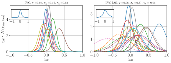
Figure 1: The distribution of the observed $\chi_{\rm eff}$ in the LVC (Left) and IAS (right) data. We have approximated each observation as a Gaussian whose mean value and $90\%$ credible interval are the values given in (The LIGO Scientific Collaboration et al., 2018a) and (Zackay et al., 2019b) respectively. The inserts show the average distribution. The title indicates the mean $\overline{\chi}$, the standard deviation $\sigma_{\chi}$ and the skewness $\gamma_{\chi}$.

We describe the data-sets in §2. We briefly discuss the models in §3 (leaving some details to a more technical Appendix B) and describe the data analysis in §4. The results are presented in 5, discussing first the results concerning the current data §5.1 and then in §5.2 we explore the question how many events are needed to distinguish between different models. We summarize our findings in §6

2 The Data

The LVC analysis of the O1-O2 runs revealed ten BBH mergers (The LIGO Scientific Collaboration et al., 2018a). Recently Venumadhav et al. (2019b) proposed a novel pipeline for the analysis of GW data. Estimated parameters of mergers identified by both pipelines are within the errors of each other (see Table A1 and Fig. 1). However, the new re-analysis of the O1 (Zackay et al., 2019b) and O2 data (Venumadhav et al., 2019a; Zackay et al., 2019a) revealed eight new BBH mergers.

In the following analysis we neglect possible mass/spin correlations. We evaluate the models over a fixed mass and compare them to the unweighted observed distribution. This is natural in the isotropic scenario and valid for field binary scenarios if tidal locking and winds operate in the same manner across the progenitors mass range. Further, given the small size of the sample, such an assumption is essential. For the same reason we neglect (see e.g. The LIGO Scientific Collaboration et al., 2018b) bias that may arise from the dependence of the GW horizon on the spin (Campanelli et al., 2006a; Roulet & Zaldarriaga, 2019).

3 The Models

3.1 Isotropic Models

The $\chi_{\rm eff}$ distribution is given by a weighted sum of two randomly oriented (isotropic) normalized spin vectors ${\bf s}_{i}$:

$$\chi_{\rm{eff-iso}}=\frac{{\bf s}_{1}\cdot\hat{\bf L}+q{\bf s}_{2}\cdot\hat{\bf L}}{1+q}\ .$$ (1)

Following Farr et al. (2017) we consider three distributions defined by the distribution of $|{\bf s_{i}}|$: flat, or dominated by either low or high spins. The probability for a given ${\bf s}$ value is:

$$p(|{\bf s_{i}}|)=\begin{cases}2(1-|{\bf s_{i}}|)&{\it low};\\ 1&{\it flat};\\ 2|{\bf s_{i}}|&{\it high}.\end{cases}$$ (2)

We use $q=1$ (varying $q$ has a minor effect, see Fig. B1 in Appendix C).

3.2 Field Binaries:

Given the complexity of binary evolution (see e.g. Qin et al., 2018; Bavera et al., 2019) we consider here a minimal model (Kushnir et al., 2016; Hotokezaka & Piran, 2017; Piran & Hotokezaka, 2018) that captures the critical ingredients during the last phase of the binary: the interplay between tidal locking, that increases and aligns the spin, and winds, that diminish it. We assume that the two processes (tidal locking and winds) are decoupled and we neglect the possible interplay between the two due to the fact that winds increase the orbital separation and this weakens the tidal force.

To account for the uncertainty in earlier phases of the evolution we consider different initial conditions for the beginning of this last phase. We briefly outline here the essential ingredients, focusing in particular on revisions that we have introduced to the model used by Piran & Hotokezaka (2018)). We consider Wolf-Rayet progenitors, as those are massive enough and have small enough radii allowing the binaries to merge within a Hubble time. However, the considerations are not limited to those and would be relevant to final stages of most field binaries, provided that their radii are small enough to fit within an orbit that can merge in a Hubble time. Numerical factors concerning the stellar model that we use in Eqs. 3-3.2 below may be different in such cases but the basic result holds.

Coalescence: We assume that at the time that the second BH forms the orbit is circular (see e.g. Hotokezaka & Piran, 2017; Mirabel, 2017) with a radius $a$. The corresponding coalescence time is:

$$t_{c}\approx 10\textrm{Gyr}~{}\brk*{\frac{2q^{2}}{1+q}}\brk*{\frac{a}{44R_{\odot}}}^{4}\brk*{\frac{m_{2}}{30M_{\odot}}}^{-3}\ .$$ (3)

We use this equation to express the orbital separation in terms of $t_{c}$. Consequently the $t_{c}$ distribution, discussed below, determines the orbital separation distribution and vice versa.

Synchronization: The synchronization of the spin of a massive star due to the tidal force exerted by the companion has been studied in different contexts by numerous authors (Brown et al., 2000; Izzard et al., 2004; Petrovic et al., 2005; Cantiello et al., 2007; van den Heuvel, 2007; Detmers et al., 2008; Eldridge et al., 2008) and more recently by Qin et al. (2018) within the context of BBH mergers. Here we characterize the effects by the time scale, $t_{syn}$, to synchronize the star spin with the orbit (Kushnir et al., 2016):

$$t_{syn}\approx 10~{}\textrm{Myr}~{}q^{-{1}/{8}}\brk*{\frac{1+q}{2q}}^{{31}/{24}}\brk*{\frac{t_{c}}{1\textrm{Gyr}}}^{{17}/{8}}\ .$$ (4)

If fully synchronized with the orbit the spin of the star is aligned and its normalized value is:

$$\chi_{syn}\approx ~{}0.5~{}q^{{1}/{4}} \brk*{\frac{1+q}{2}}^{{1}/{8}}\brk*{\frac{\epsilon}{0.075}}\brk*{\frac{R_{2}}{2R_{\odot}}}^{2}$$

$$\brk*{\frac{m_{2}}{30M_{\odot}}}^{-{13}/{8}}\brk*{\frac{t_{c}}{1\textrm{Gyr}}}^{-{3}/{8}}\ ,$$ (5)

where $\epsilon\equiv{I_{2}}/{m_{2}R^{2}_{2}}$ relates the star’s moment of inertia, $I_{2}$, to its mass and radius, $m_{2}$ and $R_{2}$.

Winds: Strong winds that operate at late phases of the stellar evolution lead to angular momentum loss, characterized by $t_{w}\equiv\chi_{*}/\dot{\chi}_{*}$, where $\chi_{*}$ is the star’s normalized aligned spin and $\dot{\chi}_{*}$ its angular momentum weighted loss rate. As mentioned earlier, we neglect the winds’ impact on the orbital separation and with this the coupling between winds and tidal locking (Qin et al., 2018). Additionally, the larger metallicity of BBHs that form recently (and hence merge with smaller $t_{c}$ values reflecting smaller initial separations) increases the effects of winds relative to BBHs that formed earlier at larger initial separations. Both effects enhance the winds’ impact. These effects will be incorporated within our model by shorter $t_{w}$ values that will indicate stronger winds.

Initial values: We consider initially synchronized stars $\chi_{*}(0)=\chi_{syn}$ or non-rotating stars $\chi_{*}(0)=0$, denoted by a subscript _syn,0 respectively. These two extreme initial conditions reflect the large uncertainty in the earlier evolution of the stars.

Evolution: The combined effects of tidal forces and winds on the stellar spin yield (Kushnir et al., 2016; Hotokezaka & Piran, 2017):

$$\frac{\textrm{d}{\chi_{*}}}{\textrm{d}{t}}=\frac{({\chi_{syn}}-\chi_{*})^{{8}/{3}}}{{t}_{syn}(t_{c})}-\frac{{\chi}_{*}}{{t_{w}}}\ .$$ (6)

We evolve $\chi_{*}$ over the lifetime of the star $t_{*}$ to obtain the final spin $\chi_{*}(t_{*})$ (see Fig.A1 in Appendix B). We fix the stellar life time at $t_{*}=0.3\textrm{Myr}$. Changing this value will merely amount to re-scaling the other time scales $t_{syn}$ and $t_{w}$. The ratio $\chi_{*}(t_{*})/{\chi_{syn}}$ depends on ${t_{w}}/{t_{syn}(t_{c})}$ and ${t_{w}}/{t_{*}}$. While the latter is of order unity, the former varies over a large range, due to the strong dependence of $t_{syn}$ on $t_{c}$ (see Eq. 4).

Collapse: If $\chi_{*}(t_{*})\leq 1$, the entire star implodes to a BH with $\chi_{{}_{BH}}=\chi_{*}(t_{*})$. If $\chi_{*}(t_{*})>1$, a fraction of the matter must be ejected carrying the excess angular momentum and $\chi_{{}_{BH}}\lesssim 1$ (Stark & Piran, 1985). Observations of massive ($>10M_{\odot}$) Galactic BHs X-ray binaries indicate that massive BHs form in situ in a direct implosion and without a kick (Mirabel, 2017). Therefore, we disregard here possible natal kicks (see e.g. Tauris et al., 2017; Mandel, 2016; Wysocki et al., 2018) that may tilt the spin and randomize it.

Single/double synchronization: In the Single Aligned (SA) scenario tidal locking and winds operate only on the secondary (the lighter) star and the resulting effective spin, $\chi_{{}_{BH,2}}$, is calculated as outlined above (see Appendix B for details). We take $\chi_{{}_{BH,1}}$ to be distributed as flat isotropic. We also consider a Double Aligned (DA) scenario in which tidal locking and winds operate on both stars in a similar manner.

Rates and delay distribution: We assume that the BBHs formation rate follows the star formation rate (SFR) (Madau & Dickinson, 2014): $R_{SFR}\brk*{z}\propto{\brk*{1+z}^{2.7}}/\{{1+[({1+z})/{2.9}]^{5.6}}\}$. This is uncertain as the progenitors are very massive stars, but we have verified (see Appendix C Fig. B2) that our predictions don’t depend strongly on the details of the BBH formation rate. In particular we also consider a formation rate that follows LGRBs that in turn follow a low metallicity population.

The mergers’ rate follows the formation rate with a time delay $t_{c}$ whose probability is assumed to be distributed as $p_{\textrm{obs}}\brk*{t_{c}}\propto t_{c}^{-1}$ for $t_{c}>t_{c,min}$. This last parameter, $t_{c,min}$ is one of the critical parameters of the model as $t_{c}$ determines the separation between the two progenitors just before the second collapse. $t_{c,min}$ corresponds, therefore to the minimal separation. The separations above this minimal one are equally distributed in the logarithm.

A detailed description of the implementation of the model and the calculation of the resulting probability distribution is given in Appendix B.

4 Data Analysis:

To estimate the validity of each model we use the Anderson & Darling (1952) test. The Anderson-Darling (AD) statistic is model dependent. To allow for a proper comparison we obtain the significance level, given in Table 1, of each model independently. For a given model, described by a distribution $p(\chi_{\rm eff})$, the significance test is performed as follows: $(i)$ We sample $\mathcal{N}=18$ noiseless data points from $p(\chi_{\rm eff})$. $(ii)$ We add an error sampled from a centered Gaussian with a standard deviation, $\overline{\sigma}_{\chi_{\rm eff}}=0.15$ (the average standard deviation in the observed $\chi_{\rm eff}$ estimates, see Table A1) to each data point. $(iii)$ We evaluate the $A^{2}$ statistic of the obtained data-set. $(iv)$ Repeating this process $10^{6}$ times gives an empirical distribution of ${A^{2}}$ from which we obtain the acceptance values (see Table 1).

	$99\%$	$90\%$	$80\%$	$70\%$	$60\%$	$50\%$	$40\%$	$30\%$	$20\%$	$10\%$	$5\%$	$4\%$	$3\%$	$2\%$	$1\%$
$\rm{SA}_{0},\rm{SA}_{syn}$	$0.18$	$0.33$	$0.44$	$0.55$	$0.66$	$0.8$	$0.96$	$1.18$	$1.49$	$2.06$	$2.69$	$2.88$	$3.15$	$3.53$	$4.19$
$\rm{DA}_{0},\rm{DA}_{syn}$	$0.18$	$0.33$	$0.45$	$0.55$	$0.67$	$0.8$	$0.96$	$1.18$	$1.5$	$2.09$	$2.71$	$2.91$	$3.18$	$3.55$	$4.24$
$(\rm{SA}_{0,syn}+\rm{DA}_{0,syn})/2$	$0.18$	$0.33$	$0.44$	$0.55$	$0.67$	$0.8$	$0.96$	$1.18$	$1.5$	$2.08$	$2.7$	$2.9$	$3.17$	$3.55$	$4.16$
$\rm{ISO}_{\rm{low}},\rm{ISO}_{\rm{flat}},\rm{ISO}_{\rm{high}}$	$0.18$	$0.33$	$0.44$	$0.55$	$0.66$	$0.79$	$0.95$	$1.16$	$1.47$	$2.05$	$2.64$	$2.85$	$3.11$	$3.49$	$4.12$

Table 1: Acceptance values of Anderson-Darling test statistic $A^{2}$ for the different models.

To test how many events are required to distinguish between two models we carry out the following procedure. We choose one distributions, denoted $p_{ref}(\chi_{\rm eff})$, as describing the “real world” and compare it to a test distribution, denoted $p_{cmp}(\chi_{\rm eff})$. To do so we obtain a data-set by sampling $\mathcal{N}$ events from $p_{ref}(\chi_{\rm eff})$. We consider those as our “observed” events and we carry out the same analysis as described earlier to test the compared model against this data-set using the AD test. We perform this over a range of sample sizes, $\mathcal{N}$.

Before comparing any model distribution to the data we must take into account the errors in the estimated $\chi_{\rm eff}$ values. To do so, for each model described by a parameter set $\lambda$, we evaluate the theoretical probability, $p_{\rm{th}}(\chi_{\rm eff};\lambda)$ (see Appendix B for details). We then account for the errors by convolving $p_{\rm{th}}(\chi_{\rm eff};\lambda)$ with a Gaussian characterized by $\bar{\sigma}_{\chi_{\rm eff}}=0.15$. The final model prediction is given by:

$$p(\chi_{\rm eff};\lambda)=\int_{-1}^{1}p_{\rm{th}}(\chi_{\rm eff}^{\prime};\lambda)\frac{e^{-\brk*{\chi_{\rm eff}-\chi_{\rm eff}^{\prime}}^{2}/2\bar{\sigma}_{\chi_{\rm eff}}^{2}}}{\sqrt{2\pi\bar{\sigma}_{\chi_{\rm eff}}}}\textrm{d}\chi_{\rm eff}^{\prime}\ .$$ (7)

As some of the events have a lower $p_{astro}$ values we have also analyzed the data taking this probability into account. Each one of the events was given a weight that is proportional to its $p_{astro}$. This has a minimal effect on the results (see Fig. 2 in Appendix C).

5 Results

We compare the current data to different models in §5.1. Given the best model in each category we then address in 5.2 the question: how many events are required to obtain a statistically significant result that will distinguish between the two categories?

5.1 Current Data

We compare the observed LVC-IAS $\chi_{\rm eff}$ distribution to the expected ones for three isotropic distributions: low, flat and high, (as defined in Farr et al., 2017) and the four field binary models: $\textrm{SA}_{0,syn}$ and $\textrm{DA}_{0,syn}$, described above. We optimize the parameters of the field binary models by performing a Maximum-Likelihood test (see Fig. 3).

Isotropic Models: Fig. 2 depicts a comparison of the distributions of the three isotropic models to the LVC-IAS data. All three isotropic models are acceptable. However, the high model is favored whereas the low model was the most favorable with the LVC data (Farr et al., 2017).

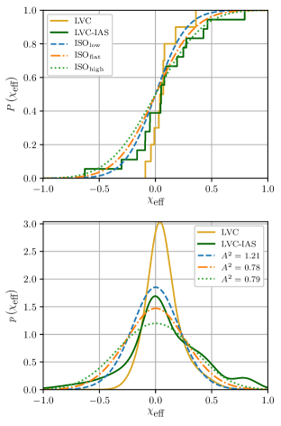
Figure 2: A comparison of the cumulative distribution, $P(\chi_{\rm eff})$, (top) and the probability density function, $p(\chi_{\rm eff})$, (bottom) of the low, flat and high isotropic models (with observation errors added) with the LVC-IAS data. The AD statistic, $A^{2}$, is marked for each model.

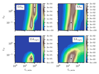
Figure 3: The likelihood $\mathcal{L}$ of the four different field binary models over a range of time-parameters, $t_{w}\in\brk[s]*{0.03,5}\textrm{Myr}$ and $t_{c,\min}\in\brk[s]*{1,1000}\textrm{Myr}$. The Maximum-Likelihood values are marked with a $*$.

Field Binaries: The models depend on three time-parameters, $t_{*},t_{c,\min}$ and $t_{w}$. We take $t_{*}=0.3\textrm{Myr}$ as the typical lifetime and use Maximum-Likelihood (see Fig. 3) to determine the best $t_{c,\min},t_{w}$ values. We find good fits (see Fig. 4) for all models. The two SA models, initially unsynchronized and synchronized, result in almost identical distributions (using different parameters). Similarly, the two DA models give identical distributions.

$\textrm{SA}_{0}$ stands out as the preferred model with the highest Maximum-Likelihood and the most reasonable physical parameters (see Piran & Hotokezaka, 2018): $t_{c,\min}=\brk[c]*{10-100~{}\textrm{Myr}}$ (corresponding, for $m_{i}\approx 30M_{\odot},\ q=1$, to $a=4-7\cdot 10^{11}~{}\textrm{cm}$) and $t_{w}=0.1-5~{}\textrm{Myr}$, reflecting a wide range of wind time scales. These values, that are on the lower side and correspond to a rather strong winds reflect probably the fact that our model underestimates somewhat the effect of winds. The Maximum-Likelihood of $\textrm{SA}_{syn}$ is comparable to the one of $\textrm{SA}_{0}$ but the former requires somewhat stronger winds ($t_{w}<0.1\textrm{Myr}$) and is valid at a more confined range. $\textrm{SA}_{0}$ and $\textrm{DA}_{0}$ have a comparable broad range of allowed physically acceptable parameters but the latter has a smaller maximal likelihood. The $\textrm{DA}_{syn}$ model has the smallest feasible parameter phase space and seems least likely. We also consider, as an example, a model that combines the two with $0.5(\textrm{SA}_{0}+\textrm{DA}_{0}$) using the best fit parameters of the $\textrm{SA}_{0}$ model. Even without optimizing the relative ratio of the two cases and the model parameters, this model fits the data slightly better than all others. When considering different stellar models the numerical factors that appear in Eqs. 4,3.2 as well as the typical stellar life time, $t_{*}$, vary. However variations in these factors will only amount to a variations in the best fit parameters and not to the quality or the overall behavior of the different scenarios.

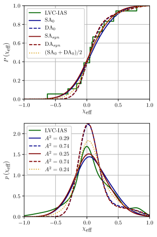
Figure 4: The cumulative distribution, $P(\chi_{\rm eff})$, (top) and the probability density function, $p(\chi_{\rm eff})$, (bottom) for the LVC-IAS data and different field binary models (using the best fitted parameters $(t_{c,\min},t_{w})\textrm{Myr}$: ${\rm{SA}}_{0}:(20,0.1)$, ${\rm{DA}}_{0}:(100,1)$, ${\rm{SA}}_{syn}:(20,0.05)$, ${\rm{DA}}_{syn}:(50,0.05)$, and a mixed model, $({\rm{SA}}_{0}+{\rm{DA}}_{0})/2$, taken with $\rm{SA}_{0}$ parameters). Note the excess of intermediate and high positive $\chi_{\rm eff}$ in these models.

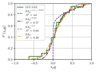
Figure 5: Same as Fig. 4 comparing between different $\textrm{SA}_{0}$ models. The curve -err,-ISO corresponds to one of the models in Piran & Hotokezaka (2018) that arise when measurements errors and an isotropic spin component for the primary BH are not taken into account. Clearly such model has no negative $\chi_{\rm eff}$ values.

Fig. 5 depicts different $\textrm{SA}_{0}$ models demonstrating the effect of the errors on the model as well as the contribution of the addition of an isotropic spin $\chi_{1}$ into the SA scenario. Both influence the resulting $\chi_{\rm eff}$ distributions giving a non-zero probability to $\chi_{\rm eff}>0.5$ and to $\chi_{\rm eff}<0$ events.

5.2 Future Estimates

As stated earlier, the current data-set is insufficient. Even the least preferred model, the low-isotropic, is consistent at $\sim 20\%$ with the data. We turn now to address the following question: Assuming that one of the models is the correct one how many mergers are needed to rule out the others? To do so we choose one of the models as the fiducial one, characterized by a distribution $p_{ref}(\chi_{\rm eff})$. We can now test any model, denoting it’s probability density as $p_{cmp}(\chi_{\rm eff})$, against the reference model. To do so we carry out the following procedure: (i) For each sample size, $\mathcal{N}$, We create an AD acceptance table for $p_{cmp}(\chi_{\rm eff})$. (ii) We sample $10^{5}$ different data-sets (numerical tests reveal that this number is sufficient) of size $\mathcal{N}$ from $p_{ref}(\chi_{\rm eff})$. (iii) We compute the average acceptance percentage of these data-sets. We repeat this procedure for $\mathcal{N}$ values ranging from $20$ to a few hundred choosing different models as the fiducial one and as the tested ones.

Within the “field evolution” models we consider the ${\rm SA}_{0}$ model and the ${\rm DA}_{0}$ with the best fit parameters over the current data-set. We compare those to the three isotropic models, low, flat and high. We also consider a mixed model in which $50\%$ of the event are ${\rm SA}_{0}$ field evolution binaries while the other $50\%$ are flat isotropic.

Fig. 6 (top) depicts the resulting acceptance (1-rejection) probability of different tested models. It appears that $50-100$ ($150-250$) mergers are require to distinguish the ${\rm SA}_{0}$ model from the isotropic ones at the $5\%$ ($1\%$) confidence level. The ${\rm DA}_{0}$ model includes more positive high spin events and fewer negative spin ones. Hence, as expected, it is easier to distinguish it from the isotropic models. As shown in Fig. 6 (bottom) $30-60$ ($50-120$) mergers are sufficient to distinguish between the ${\rm DA}_{0}$ model and the different isotropic models at the $5\%$ ($1\%$) confidence level. A caveat in the above estimate is that it cannot account for possible variations in the best fit parameters of the field binaries models ${\rm SA}_{0}$, ${\rm DA}_{0}$ that may arise in a large data-set. The situation is more complicated when we consider mixed models that combine both field binaries and capture. A few hundred mergers are needed to distinguish between these models and “pure” field binaries or “pure” capture models.

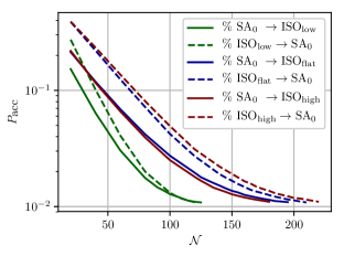
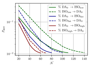
Figure 6: Probability of acceptance, $P_{acc}$, (or rejection that is $1-P_{acc}$) level of different models as a function of the number $\mathcal{N}$ of events detected. We compare the field evolution models, $\rm{SA}_{0}$ (top) and $\rm{DA}_{0}$ (bottom), with the three isotropic models low flat and high. Solid curves assume that the field evolution model describes the ”real world” and depict the acceptance significance of the isotropic models. Dashed curves assume that the isotropic models are the correct one and estimate the acceptance level for the respective field model. As expected it is easier to distinguish between the low isotropic and the $\rm{SA}_{0}$ model than to distinguish between the flat and high isotropic models and $\rm{SA}_{0}$. Further, a fewer events are needed (as compared to $\rm{SA}_{0}$) to distinguish between the $\rm{DA}_{0}$ field evolution model and the isotropic models

One may wonder whether a few strong events whose $\chi_{\rm eff}$ can be determined at a higher accuracy can change these conclusions. To check this we carried out the same test using now different values of $\bar{\sigma}_{\chi_{\rm eff}}$, the standard deviation in the estimation of $\chi_{\rm eff}$ (see Fig. 7). As expected fewer events would suffice with a lower $\bar{\sigma}_{\chi_{\rm eff}}$. If $\bar{\sigma}_{\chi_{\rm eff}}$ is a quarter of its current value $25-50$ ($80-120$) events are needed to distinguish at the $5\%$ ($1\%$) confidence level between the ${\rm SA}_{0}$ model and the isotropic ones.

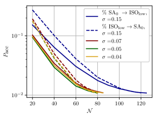
Figure 7: The acceptance probability as a function of the number of mergers (same as Fig. 6) between the $\rm{SA}_{0}$ and the low isotropic models. Solid lines test the acceptance of a low isotropic model assuming that the correct model is $\rm{SA}_{0}$. Dashed lines consider the opposite. The standard deviation in measuring $\chi_{\rm eff}$ varies from 0.15 as in the current observed sample to 0.04.

6 Conclusions

The observed low effective spins, that were centered around $0$, in the LVC O1-O2 sample favored low spin isotropic distributions (Farr et al., 2017) and hence capture scenarios. We have shown here that while the combined LVC-IAS data-set that includes a high $\chi_{\rm eff}$ binary, cannot rule out any model it favors field binaries over capture.

Within the field binary models the high $\chi_{\rm eff}$ merger implies a significant fraction of short ($t_{c}\sim 20\textrm{Myr}$) mergers, namely BBHs that at formation had small, but reasonable ($4-7\times 10^{11}\textrm{cm}$), separations. Overall the LVC-IAS sample brackets nicely the phase space of the field binary model with $10\textrm{Myr}\lesssim t_{c,min}\lesssim 100\textrm{Myr}$, $0.05\textrm{Myr}\lesssim t_{w}\lesssim 5\textrm{Myr}$.

While the isotropic scenario is disfavored it is not ruled out. Among those models the high variant becomes the most favorable and the low the least. It is interesting to note that recently Romero-Shaw et al. (2019) have shown that the eccentricity of all the events in the LVC sample are smaller than $0.02$ to $0.05$, whereas a capture scenario suggests that $5\%$ of the events should have larger eccentricity. Again, while this result doesn’t rule out the capture scenarios they support our findings. Clearly, a mixture of field binaries and capture is possible. In this case we expect that the former will be dominant. However, given the limited data we didn’t explore this possibility here. Considering future observations we note that the hallmark of the field binaries scenario is a preferably positive $\chi_{\rm eff}$ distribution with a few large positive $\chi_{\rm eff}$ mergers. At the same time, unless kicks are very significant and dominate the BHs spin distribution, large negative $\chi_{\rm eff}$ will pose a problem for the field binary model. We have shown that for the models considered here we will need $30-250$ events, depending on the details of the model and the level of confidence required to distinguish between the two scenarios. Higher S/N data that has a better determined $\chi_{\rm eff}$ value would require a fewer events. Hundreds of events will be needed to determine the ratio of capture to field evolution events in mixed model that includes both capture and field binaries, or to distinguish those from pure capture or pure field evolution models.

Appendix A Data

Event	${m_{1}}/{M_{\odot}}$		${m_{2}}/{M_{\odot}}$		$\chi_{\rm eff}$		$p_{\mathrm{astro}}$
	LVC	IAS	LVC	IAS	LVC	IAS	IAS
GW150914	$35.6^{+4.8}_{-3.0}$	$35.9^{+4.47}_{-4.45}$	$30.6^{+3.0}_{-4.4}$	$29.6^{+3.5}_{-3.6}$	$-0.01^{+0.12}_{-0.13}$	$-0.05^{+0.11}_{-0.11}$	$*$
GW151012	$23.3^{+14.0}_{-5.5}$	$27.3^{+12.03}_{-11.89}$	$13.6^{+4.1}_{-4.8}$	$12.11^{+4.25}_{-4.2}$	$0.04^{+0.28}_{-0.19}$	$0.05^{+0.23}_{-0.23}$	$>0.99$
GW151226	$13.7^{+8.8}_{-3.2}$	$16.4^{+7.53}_{-7.5}$	$7.7^{+2.2}_{-2.6}$	$7.53^{+2.45}_{-2.47}$	$0.18^{+0.20}_{-0.12}$	$0.27^{+0.19}_{-0.19}$	$*$
GW170104	$31.0^{+7.2}_{-5.6}$	$30.17^{+5.95}_{-5.96}$	$20.1^{+4.9}_{-4.5}$	$19.6^{+3.89}_{-3.85}$	$-0.04^{+0.17}_{-0.20}$	$-0.09^{+0.16}_{-0.16}$	$>0.99$
GW170608	$10.9^{+5.3}_{-1.7}$	$17.4^{+11.43}_{-11.45}$	$7.6^{+1.3}_{-2.1}$	$5.8^{+2.66}_{-2.66}$	$0.03^{+0.19}_{-0.07}$	$0.25^{+0.3}_{-0.31}$	$>0.99$
GW170729	$50.6^{+16.6}_{-10.2}$	$50.3^{+12.42}_{-11.5}$	$34.3^{+9.1}_{-10.1}$	$34.6^{+9.05}_{-9.03}$	$0.36^{+0.21}_{-0.25}$	$0.43^{+0.21}_{-0.21}$	$>0.99$
GW170809	$35.2^{+8.3}_{-6.0}$	$36.1^{+7.8}_{-7.76}$	$23.8^{+5.2}_{-5.1}$	$23.6^{+4.95}_{-4.94}$	$0.07^{+0.16}_{-0.16}$	$0.08^{+0.19}_{-0.19}$	$>0.99$
GW170814	$30.7^{+5.7}_{-3.0}$	$31.0^{+4.53}_{-4.53}$	$25.3^{+2.9}_{-4.1}$	$24.98^{+3.29}_{-3.29}$	$0.07^{+0.12}_{-0.11}$	$0.05^{+0.11}_{-0.11}$	$>0.99$
GW170818	$35.5^{+7.5}_{-4.7}$	$35.4^{+5.92}_{-5.91}$	$26.8^{+4.3}_{-5.2}$	$26.87^{+4.59}_{-4.6}$	$-0.09^{+0.18}_{-0.21}$	$0.05^{+0.2}_{-0.2}$	$>0.99$
GW170823	$39.6^{+10.0}_{-6.6}$	$39.5^{+7.34}_{-7.43}$	$29.4^{+6.3}_{-7.1}$	$28.5^{+5.91}_{-5.91}$	$0.08^{+0.20}_{-0.22}$	$0.09^{+0.22}_{-0.22}$	$>0.99$
GW170121	$-$	$31.8^{+6.56}_{-6.58}$	$-$	$23.9^{+5.07}_{-5.05}$	$-$	$-0.3^{+0.29}_{-0.29}$	$>0.99$
GW170727	$-$	$40.1^{+8.34}_{-8.35}$	$-$	$29.1^{+6.6}_{-6.63}$	$-$	$-0.09^{+0.32}_{-0.33}$	$0.98$
GW170304	$-$	$42.9^{+9.79}_{-9.73}$	$-$	$31.6^{+7.5}_{-7.5}$	$-$	$0.19^{+0.31}_{-0.31}$	$0.985$
GW170817A	$-$	$56^{+16}_{-10}$	$-$	$40^{+10}_{-11}$	$-$	$0.5^{+0.2}_{-0.2}$	$0.86$
GW170425	$-$	$46.7^{+14.9}_{-14.92}$	$-$	$29.9^{+9.87}_{-9.91}$	$-$	$0.05^{+0.42}_{-0.42}$	$0.77$
GW151216	$-$	$32.3^{+9.7}_{-9.7}$	$-$	$20.47^{+5.76}_{-5.76}$	$-$	$0.8^{+0.18}_{-0.18}$	$0.71$
GW170202	$-$	$29.87^{+11.46}_{-11.45}$	$-$	$14.32^{+4.48}_{-4.48}$	$-$	$-0.16^{+0.34}_{-0.34}$	$0.68$
GW170403	$-$	$45.5^{+10.25}_{-10.25}$	$-$	$32.7^{+8.29}_{-8.25}$	$-$	$-0.63^{+0.39}_{-0.38}$	$0.56$

Table A1: Parameters of the BBH mergers detected during LVC’s O1 and O2 by LVC (left columns, The LIGO Scientific Collaboration et al. (2018a)) and IAS (right columns, Venumadhav et al. (2019a); Zackay et al. (2019a)). The parameters are median values with $90\%$ credible intervals.

Appendix B The Model Distribution for Field Binaries

The model distribution, $p_{th}\brk*{\chi_{\rm eff};\lambda}$,

$\lambda=\brk[c]*{{\rm{SA}_{0,syn}/\rm{DA}_{0,syn}},m_{1},m_{2},t_{c,\min},t_{w},t_{*}}$, is derived under the assumptions given in the main text.

We take the BBH formation rate per volume element per unit comoving time, $R\brk*{z}$, to follow the star formation rate (we also consider other rates, see Appendix C).

The mergers’ rate follows the formation rate with a delay $t_{c}$ whose probability is assumed to be $p_{obs}\brk*{t_{c}}\propto t_{c}^{-1}$ for $t_{c}>t_{c,\min}$. This allows us to define the probability that the merger occurred at redshift $z_{c}$ as:

$$p\brk*{z_{c}}=\frac{1}{t_{c}\brk*{z_{c}}}\frac{R\brk*{z_{c}}}{1+z_{c}}\frac{\rm{d}t_{c}}{\rm{d}z_{c}}\ .$$ (B1)

We approximate, implicitly, that all mergers take place now (relaxing this assumption and assuming that the mergers take place between $z=0$ and $z=0.5$ doesn’t change our results).

For a given $t_{c}$ and fixed $t_{w},t_{*}$ we compute the final stellar spin, $\chi_{*}(t_{*})$ by integrating (Eq. 5 of the main text):

$$\frac{\textrm{d}{\chi_{*}}}{\textrm{d}{t}}=\frac{({\chi_{syn}}-\chi_{*})^{{8}/{3}}}{{t}_{syn}(t_{c})}-\frac{{\chi}_{*}}{{t_{w}}}\ ,$$ (B2)

from 0 to $t_{*}$. As initial conditions we take

$$\chi_{*}(0)=\begin{cases}0&\mbox{unsynchronized }\ ,\\ \chi_{syn}&\mbox{synchronized }\ .\end{cases}$$ (B3)

Fig. A1 depicts the results of this integration in terms of $\chi_{*}/\chi_{syn}$, as a function of $t/t_{w}$ for different ratios of $\tilde{t}_{syn}\equiv\chi_{syn}^{-5/3}(t_{syn}/t_{w}$).

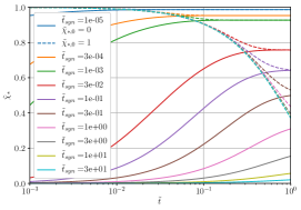
Figure A1: $\tilde{\chi}\equiv\chi_{*}/\chi{syn}$ as a function of $\tilde{t}\equiv t/t_{w}$ for different values of $\tilde{t}_{syn}\equiv\chi_{syn}^{-5/3}(t_{syn}/t_{w})$.

The BH spin after the collapse is then given by:

$$\chi_{{}_{BH}}=\min\brk[c]*{\chi_{*}(t_{*}),1}\ .$$ (B4)

Under the assumption that $\chi_{{}_{BH}}$ is deterministic w.r.t it’s parameters, we may write it’s distribution using the chain rule:

$$p\brk*{\chi_{{}_{BH}};\lambda}=\frac{1}{t_{c}\brk*{z_{c}}}\frac{R\brk*{z_{c}}}{1+z_{c}}\frac{\rm{d}\chi_{{}_{BH}}}{\rm{d}t_{c}}\frac{\rm{d}t_{c}}{\rm{d}z_{c}},$$ (B5)

where we calculate numerically the derivative ${\rm{d}\chi_{{}_{BH}}}/{\rm{d}t_{c}}$, following the integration of Eq. 6 above.

To obtain the final $\chi_{\rm eff}$ distribution:

$$\chi_{\rm eff}=\frac{\chi_{{}_{BH,1}}+q\chi_{{}_{BH,2}}}{\brk*{1+q}}\ ,$$ (B6)

we consider the different scenarios separately.

• SA: $\chi_{{}_{BH,1}}$ is distributed as flat isotropic and $\chi_{{}_{BH,2}}$ is given by equation (B5). To find the resulting distribution of $\chi_{\rm eff}$ we sample each (from the respective distribution) and calculate the empirical distribution of their weighted sum.

• DA: Using the above procedure, for a given $t_{c}$ ,we calculate $\chi_{{}_{BH,1}}$ and $\chi_{{}_{BH,2}}$. Using the numerical values of the derivative, ${\rm{d}\chi_{eff}}/{\rm{d}t_{c}}$, we obtain the distribution:

  $$p\brk*{\chi_{eff};\lambda}=\frac{1}{t_{c}\brk*{z_{c}}}\frac{R\brk*{z_{c}}}{1+z_{c}}\frac{\rm{d}\chi_{eff}}{\rm{d}t_{c}}\frac{\rm{d}t_{c}}{\rm{d}z_{c}}\ .$$ (B7)

Appendix C Additional Tests

The Mass Distribution: The masses used in the estimates are the average values of the sample: $\overline{m}_{1}=38M_{\odot}$ and $\overline{m}_{2}=24M_{\odot}$. To explore the effect of the different masses, we also use the masses of the observed events and sample over the mass distribution. The results are shown in Fig. B1 for the SA distribution and for the isotropic models whose $\chi_{\rm eff}$ distribution is affected (becomes broader) when mass ratio is taken into account. We find that the results are almost the same as those obtained using the average mass and mass ratio.

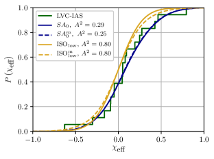
Figure B1: The models evaluated using a mixture of mass ratios, $m_{1},m_{2}$. That is for each model we find it’s prediction to each of the $N=18$ observed masses and consider the average of this predictions as the final probability of the model. We denote the mixture probabilities a superscript $m$.

The Event Rate: We use the star formation rate as the event rate for the formation of BBH. We also consider the possibility that BBH follow the long GRB (LGRB) rate, as it was suggested that long GRBs indicate the formation of a BBH (Piran & Hotokezaka, 2018), and a (ad hoc) constant formation rate. Fig. B2 demonstrates that the resulting distribution is practically independent of the assumption on the SFR.

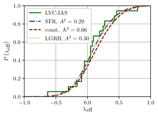
Figure B2: The effect of the rate function, $R\brk*{z}$ on the model prediction. All rates are evaluated under the $\rm{SA}_{0}$ scenario.

$p_{astro}$ weight: The observed events are given a probability that the event is of astrophysical, $p_{astro}$. Weighting the events using this value to obtain the observed distribution does not affect the goodness of fit ($A^{2}$ score) of our models, see Fig. B3.

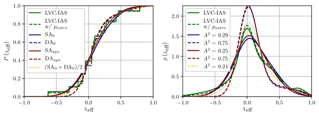
Figure B3: The effect of weighting the observed events by $p_{astro}$ on the obtained observed distribution and goodness of fit to the models (calculated with the same parameters).

References

- Anderson & Darling (1952) Anderson T. W., Darling D. A., 1952, Ann. Math. Statist., 23, 193
- Antonini & Rasio (2016) Antonini F., Rasio F. A., 2016, ApJ, 831, 187
- Bartos et al. (2017) Bartos I., Kocsis B., Haiman Z., Márka S., 2017, ApJ, 835, 165
- Bavera et al. (2019) Bavera S. S., et al., 2019, arXiv e-prints, p. arXiv:1906.12257
- Belczynski et al. (2016) Belczynski K., Holz D. E., Bulik T., O’Shaughnessy R., 2016, Nature, 534, 512
- Belczynski et al. (2017) Belczynski K., et al., 2017, preprint, (arXiv:1706.07053)
- Bird et al. (2016) Bird S., Cholis I., Muñoz J. B., Ali-Haïmoud Y., Kamionkowski M., Kovetz E. D., Raccanelli A., Riess A. G., 2016, Physical Review Letters, 116, 201301
- Blinnikov et al. (2016) Blinnikov S., Dolgov A., Porayko N. K., Postnov K., 2016, J. Cosmology Astropart. Phys, 11, 036
- Brown et al. (2000) Brown G. E., Lee C. H., Wijers R. A. M. J., Lee H. K., Israelian G., Bethe H. A., 2000, New A, 5, 191
- Campanelli et al. (2006a) Campanelli M., Lousto C. O., Zlochower Y., 2006a, Phys. Rev. D, 74, 041501
- Campanelli et al. (2006b) Campanelli M., Lousto C. O., Marronetti P., Zlochower Y., 2006b, Physical Review Letters, 96, 111101
- Cantiello et al. (2007) Cantiello M., Yoon S. C., Langer N., Livio M., 2007, A&A, 465, L29
- Detmers et al. (2008) Detmers R. G., Langer N., Podsiadlowski P., Izzard R. G., 2008, A&A, 484, 831
- Eldridge et al. (2008) Eldridge J. J., Izzard R. G., Tout C. A., 2008, MNRAS, 384, 1109
- Farr et al. (2017) Farr W. M., Stevenson S., Miller M. C., Mandel I., Farr B., Vecchio A., 2017, Nature, 548, 426 EP
- Fragione & Kocsis (2018) Fragione G., Kocsis B., 2018, Phys. Rev. Lett., 121, 161103
- Fragione et al. (2019) Fragione G., Grishin E., Leigh N. W. C., Perets H. B., Perna R., 2019, MNRAS, 488, 47
- Hoang et al. (2018) Hoang B.-M., Naoz S., Kocsis B., Rasio F. A., Dosopoulou F., 2018, ApJ, 856, 140
- Hotokezaka & Piran (2017) Hotokezaka K., Piran T., 2017, ApJ, 842, 111
- Ioka et al. (1998) Ioka K., Chiba T., Tanaka T., Nakamura T., 1998, Phys. Rev. D, 58, 063003
- Ivanova et al. (2013) Ivanova N., et al., 2013, A&A Rev., 21, 59
- Izzard et al. (2004) Izzard R. G., Ramirez-Ruiz E., Tout C. A., 2004, MNRAS, 348, 1215
- Kashlinsky (2016) Kashlinsky A., 2016, ApJ, 823, L25
- Kocsis & Levin (2012) Kocsis B., Levin J., 2012, Phys. Rev. D, 85, 123005
- Kushnir et al. (2016) Kushnir D., Zaldarriaga M., Kollmeier J. A., Waldman R., 2016, Monthly Notices of the Royal Astronomical Society, 462, 844
- Madau & Dickinson (2014) Madau P., Dickinson M., 2014, Annual Review of Astronomy and Astrophysics, 52, 415
- Mandel (2016) Mandel I., 2016, MNRAS, 456, 578
- Mandel & O’Shaughnessy (2010) Mandel I., O’Shaughnessy R., 2010, Classical and Quantum Gravity, 27, 114007
- Mandel & de Mink (2016) Mandel I., de Mink S. E., 2016, MNRAS, 458, 2634
- Marchant et al. (2016) Marchant P., Langer N., Podsiadlowski P., Tauris T. M., Moriya T. J., 2016, A&A, 588, A50
- McKernan et al. (2018) McKernan B., et al., 2018, ApJ, 866, 66
- Miller & Lauburg (2009) Miller M. C., Lauburg V. M., 2009, ApJ, 692, 917
- Mirabel (2017) Mirabel I. F., 2017, in Gomboc A., ed., IAU Symposium Vol. 324, New Frontiers in Black Hole Astrophysics. pp 303–306 (arXiv:1611.09266), doi:10.1017/S1743921316012904
- O’Leary et al. (2009) O’Leary R. M., Kocsis B., Loeb A., 2009, MNRAS, 395, 2127
- O’Leary et al. (2016) O’Leary R. M., Meiron Y., Kocsis B., 2016, The Astrophysical Journal Letters, 824, l12
- O’Shaughnessy et al. (2017) O’Shaughnessy R., Gerosa D., Wysocki D., 2017, Physical Review Letters, 119, 011101
- Petrovic et al. (2005) Petrovic J., Langer N., van der Hucht K. A., 2005, A&A, 435, 1013
- Phinney (1991) Phinney E. S., 1991, ApJ, 380, L17
- Piran & Hotokezaka (2018) Piran T., Hotokezaka K., 2018, arXiv e-prints, p. arXiv:1807.01336
- Portegies Zwart & McMillan (2000) Portegies Zwart S. F., McMillan S. L. W., 2000, ApJ, 528, L17
- Postnov & Mitichkin (2019) Postnov K. A., Mitichkin N. A., 2019, J. Cosmology Astropart. Phys, 2019, 044
- Qin et al. (2018) Qin Y., Fragos T., Meynet G., Andrews J., Sørensen M., Song H. F., 2018, A&A, 616, A28
- Rodriguez et al. (2016) Rodriguez C. L., Zevin M., Pankow C., Kalogera V., Rasio F. A., 2016, The Astrophysical Journal, 832, L2
- Rodriguez et al. (2018) Rodriguez C. L., Amaro-Seoane P., Chatterjee S., Kremer K., Rasio F. A., Samsing J., Ye C. S., Zevin M., 2018, Phys. Rev. D, 98, 123005
- Romero-Shaw et al. (2019) Romero-Shaw I. M., Lasky P. D., Thrane E., 2019, arXiv e-prints, p. arXiv:1909.05466
- Roulet & Zaldarriaga (2019) Roulet J., Zaldarriaga M., 2019, Monthly Notices of the Royal Astronomical Society, 484, 4216
- Sasaki et al. (2016) Sasaki M., Suyama T., Tanaka T., Yokoyama S., 2016, Physical Review Letters, 117, 061101
- Secunda et al. (2019) Secunda A., Bellovary J., Mac Low M.-M., Ford K. E. S., McKernan B., Leigh N. W. C., Lyra W., Sándor Z., 2019, ApJ, 878, 85
- Sigurdsson & Hernquist (1993) Sigurdsson S., Hernquist L., 1993, Nature, 364, 423
- Stark & Piran (1985) Stark R. F., Piran T., 1985, Physical Review Letters, 55, 891
- Stevenson et al. (2017) Stevenson S., Vigna-Gómez A., Mandel I., Barrett J. W., Neijssel C. J., Perkins D., de Mink S. E., 2017, Nature Communications, 8, 14906
- Stone et al. (2017) Stone N. C., Metzger B. D., Haiman Z., 2017, MNRAS, 464, 946
- Tauris et al. (2017) Tauris T. M., et al., 2017, ApJ, 846, 170
- The LIGO Scientific Collaboration et al. (2018b) The LIGO Scientific Collaboration et al., 2018b, arXiv e-prints,
- The LIGO Scientific Collaboration et al. (2018a) The LIGO Scientific Collaboration et al., 2018a, arXiv e-prints,
- The LIGO Scientific Collaboration et al. (2018c) The LIGO Scientific Collaboration et al., 2018c, arXiv e-prints, p. arXiv:1811.12940
- Tutukov & Yungelson (1993) Tutukov A. V., Yungelson L. R., 1993, MNRAS, 260, 675
- Venumadhav et al. (2019a) Venumadhav T., Zackay B., Roulet J., Dai L., Zaldarriaga M., 2019a, arXiv e-prints, p. arXiv:1904.07214
- Venumadhav et al. (2019b) Venumadhav T., Zackay B., Roulet J., Dai L., Zaldarriaga M., 2019b, Phys. Rev. D, 100, 023011
- Wiktorowicz et al. (2019) Wiktorowicz G., Wyrzykowski Ł., Chruslinska M., Klencki J., Rybicki K. A., Belczynski K., 2019, ApJ, 885, 1
- Wysocki et al. (2018) Wysocki D., Gerosa D., O’Shaughnessy R., Belczynski K., Gladysz W., Berti E., Kesden M., Holz D. E., 2018, Phys. Rev. D, 97, 043014
- Zackay et al. (2019a) Zackay B., Dai L., Venumadhav T., Roulet J., Zaldarriaga M., 2019a, arXiv e-prints, p. arXiv:1910.09528
- Zackay et al. (2019b) Zackay B., Venumadhav T., Dai L., Roulet J., Zaldarriaga M., 2019b, Phys. Rev. D, 100, 023007
- van den Heuvel (2007) van den Heuvel E. P. J., 2007, in di Salvo T., Israel G. L., Piersant L., Burderi L., Matt G., Tornambe A., Menna M. T., eds, American Institute of Physics Conference Series Vol. 924, The Multicolored Landscape of Compact Objects and Their Explosive Origins. pp 598–606 (arXiv:0704.1215), doi:10.1063/1.2774916