An optical search for transients lasting a few seconds

Abstract

Using a prototype of the Tomo-e Gozen wide-field CMOS mosaic camera, we acquire wide-field optical images at a cadence of 2 Hz and search them for transient sources of duration 1.5 to 11.5 seconds. Over the course of eight nights, our survey encompasses the equivalent of roughly two days on one square degree, to a fluence equivalent to a limiting magnitude about $V=15.6$ in a 1-second exposure. After examining by eye the candidates identified by a software pipeline, we find no sources which meet all our criteria. We compute upper limits to the rate of optical transients consistent with our survey, and compare those to the rates expected and observed for representative sources of ephemeral optical light.

1 Introduction

The sky is filled with objects which appear eternal to the average human eye. True, the position and brightness of the planets change from week to week, and that of the Moon from night to night, but every generation of humans has seen the same Moon. To ancient skywatchers, the fixed stars seemed even more constant. On the rare occasions when a comet might appear for a few months, its ephemeral nature was held as a reason that it must be an atmospheric phenomenon and not a true member of the celestial sphere.

Over the past few centuries, astronomers have recognized that some stars do vary appreciably in brightness, and all drift across the sky, albeit slowly. Systematic surveys starting in the nineteenth century found evidence for stellar variation on timescales of years, days, and even hours. In recent decades, improving technology in detectors, telescope control systems, and data analysis has led to the creation of larger and larger catalogs of variable stars. Astronomers have also detected many transient objects: novae, supernovae, gamma-ray bursts (GRBs), fast radio bursts, and tidal disruption events, to name just a few.

Despite these efforts, some regions of parameter space remain largely unexplored. In particular, objects which appear only once for durations of just a few seconds – in a word, “flashes” – have escaped serious study. The compilation of studies presented by [Berger et al. (2013)], for example, includes no projects sensitive to flashes shorter than 20 minutes. There are at least three factors which make it difficult to look for sources which emit for only a few minutes, let alone a few seconds. First, some detectors are not designed to operate at high cadence; large format CCDs require long readout times to produce images with low noise. Second, in order to eliminate false positives, it is beneficial to acquire at least two, if not three, measurements of a single event before it disappears; yet it is difficult to accumulate a reasonable signal-to-noise ratio in such short exposures. Finally, long stretches of high-cadence measurements will produce a very large dataset, increasing the time and effort required to identify and confirm real transients.

Our effort was inspired by the development of large CMOS detectors which yield low noise even when read out several times per second. Placing a mosaic of such devices onto the focal plane of a Schmidt telescope creates an instrument which can sample large areas of the sky with high cadence, and designing a pipeline to analyze the large volume of data carefully reduces the amount of human oversight required to detect transient sources reliably. In section 2, we describe our equipment and the methods used to acquire images. The processing of those images into calibrated lists of stars is explained in section 3. We discuss the criteria by which transient objects are chosen from the star lists in Section 4, and conclude that no objects satisfy all our conditions. In section 5, we use our null result to compute upper limits on the rates of transient sources per square degree. We explain how to convert the rates into volumetric units in section 6, and briefly compare them to observed and expected rates from the literature for two types of source. We compare our survey to three others which sample timescales of a few seconds in section 7.

We assume throughout this work a cosmology with $H_{0}=69.6$ km/s/Mpc, $\Omega_{M}=0.286$ and $\Omega_{\Lambda}=0.714$.

2 Observations

All images were acquired with the 105-cm Schmidt Telescope at Kiso Observatory, at $35^{\circ}47{{}^{\prime}}50{\hbox to0.0pt{.\hss}}{{}^{\prime\prime}}0$ North, $137^{\circ}37^{\prime}31{\hbox to0.0pt{.\hss}}{{}^{\prime\prime}}5$ East in the WGS84 system, and an altitude of 1132 m. Light was focused on an early version of the Tomo-e Gozen camera (Sako et al., 2016, 2018), referred to hereafter as Tomo-e PM (for “Prototype Model”). This prototype had 8 CMOS sensors installed on the focal plane, each with $2000\times 1128$ pixels of size $19\ \mu$m on a side. The plate scale was approximately $1{\hbox to0.0pt{.\hss}}{{}^{\prime\prime}}19$ arcseconds per pixel. Each chip subtended an area of approximately $39.7\times 22.4$ arcminutes, and the set of eight covered a total of about 1.9 square degrees, aligned in a row running east to west. Image frames were obtained by a rolling read operation at two frames per second; since the pixel reset time is only 0.1 milliseconds, the exposure time of each frame was approximately 0.5 seconds. No filters were placed between the sensors and the sky, so the detectors measured light over the range $370$ to $730$ nm, with a peak quantum efficiency of $0.68$ at $\lambda=500$ nm.

The data analyzed herein were gathered during eight nights in March and April of 2016; see Table 1 for a list of the nights. In order to minimize the number of artificial satellites and space debris in our images, we aimed the telescope in the direction of the the Earth’s shadow. During each night, the pointing of the telescope gradually moved west to follow the shadow; figure 1 shows the area covered during each night. The center of this region is approximately at ${\rm RA}=190^{\circ}$, ${\rm Dec}=-8^{\circ}$, which corresponds to galactic coordinates ${\rm\ell}=298^{\circ}$, ${b}=+55^{\circ}$ and ecliptic ${\rm long}=192^{\circ}$, ${\rm lat}=-3^{\circ}$. It is far from the plane of the Milky Way, but close to the plane of the ecliptic.

Table 1: Nights of observation

Date	hours	FWHM (arcsec)	weather
2016 March 15	8.4	$4-5$	good
2016 March 16	6.7	$3-5$	brief clouds
2016 March 17	7.9	$3-4$	mediocre
2016 March 30	5.0	$4-7$	mediocre
2016 April 08	6.5	$4-6$	good
2016 April 09	5.3	$3-4$	light clouds
2016 April 11	6.5	$5-8$	good
2016 April 14	6.2	$5-8$	light clouds

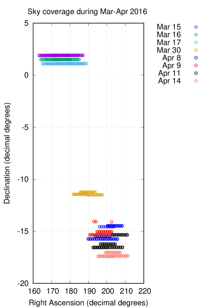
Figure 1: Sky coverage during eight nights in March-April, 2016. A different color is used for each night. Each symbol shows the center of a field, but the size of the symbols is not equal to the area of each field.

3 Processing the images

The real-time electronics collect the information from each sensor and package it into units we call “chunks,” which consist of 360 individual images (180 seconds of data at 2 Hz). As described below, we sometimes treat the information from a single chunk as a unit for calibration.

We list below the steps involved in converting each raw image from a single sensor into a list of astrometrically and photometrically calibrated objects.

1. Following the method described in Ohsawa et al. (2016), we create a simple model of the bias for each image; it has a structure which repeats every four rows. We subtract this bias from the raw image pixels.

2. We do not perform any flatfielding.

3. Using the stars and phot routines of the XVista package (Treffers & Richmond, 1989; Richmond, 2017), we identify objects with peaks significantly above the sky level and perform aperture photometry. Objects with sizes much smaller or larger than the typical stellar FWHM are excluded. We measure the flux of each object within circular apertures of two sizes: one fixed at 10 pixels ($11{\hbox to0.0pt{.\hss}}{{}^{\prime\prime}}8$) and one which varied from image to image, equal to $1.5$ times the FWHM of the image. The result of this stage is one list of stars per image, with (row, col) positions and instrumental magnitudes on an arbitrary scale.

4. Objects detected at least twice in the images of a single chunk are combined into an ensemble. These objects are subjected to inhomogeneous ensemble photometry (Honeycutt, 1992), bringing them to a single photometric zeropoint. This procedure creates a set of robust statistics, such as the photometric uncertainty as a function of instrumental magnitude.

5. We calibrate the ensemble averages of each object astrometrically against the UCAC4 (Zacharias et al., 2013), and photometrically against the UCAC4’s $V-$band magnitudes; recall that our measurements are unfiltered. This provides accurate measurements for stars which appear in most of the images of the chunk; in other words, for ordinary stars which do not vary on short timescales.

6. The objects detected in each individual image are also calibrated against the UCAC4, astrometrically and photometrically, in a similar manner. These results will be less accurate, but provide measurements for transient objects which might not be included in the ensembles.

7. We create a set of diagnostic graphs and tables, summarizing the properties of objects in each chunk.

We employed a simple first-order model to match the (x, y) positions of stars on each sensor to the (RA, Dec) positions from the UCAC4 catalog. The typical solution involved 30 to 50 stars and yielded residuals of size $\sim 0{\hbox to0.0pt{.\hss}}{{}^{\prime\prime}}5$, adequate for our purposes. See Figure 2 for details.

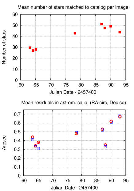
Figure 2: Properties of astrometric solutions in March and April, 2016. In the lower panel, mean residuals in RA are shown as red circles, in Dec by blue squares.

We found that using photometric apertures which varied with the seeing produced better results than using fixed apertures, not surprising given the considerable variations in FWHM over the course of some of our nights. Depending on the conditions, bright stars ($V\sim 11$) showed scatter of 0.02 to 0.03 mag, while measurements of faint stars ($V\sim 16$) varied by 0.08 to 0.12 mag from image to image. Figure 3 shows examples under good and adverse conditions. Note that our very short exposures mean that scintillation noise can contribute significantly to the noise floor at moderate airmass.

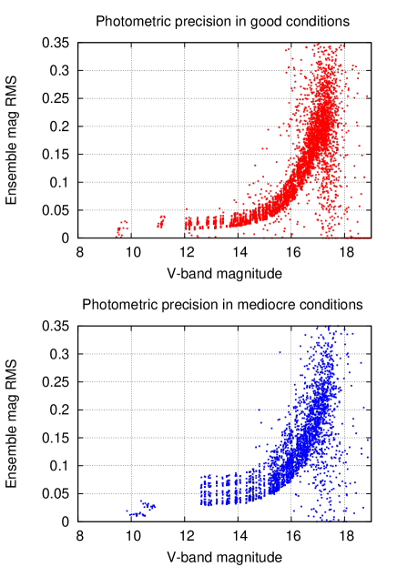
Figure 3: Scatter in repeated measurements as a function of magnitude. Top panel: good conditions, 2016 Mar 15 around JD 2457463.06; bottom panel: poor conditions, 2016 Mar 17 around JD 2457465.06

The pipeline produces two lists of stars as its main output. One is based on the ensemble of stars within each chunk of images; the other is a list of every object detected in each individual image. Each list is calibrated in position and magnitude against the UCAC4 catalog. The pipeline also produces a set of diagnostic graphs to help us determine the quality of each night.

4 Search for transients

Running the pipeline takes a significant amount of computing power and time. We designed our algorithm which searches for transient objects to operate on the star lists created by the pipeline. Since the data volume is much smaller (by factors of $\sim 100$), the time to search, check, and if necessary re-search is much smaller.

Our method is based on measurements made within a single chunk of data: 360 consecutive images spanning 180 seconds. As described below, this can cause the method to miss a very small fraction of very brief transients; however, we accept this small drawback in return for a significant simplication in the bookkeeping.

We scan through all objects detected within the chunk and subject them to a series of tests. An object which fails any test is discarded. In order to pass these tests,

1. an object must be detected between 3 and 20 times within a single chunk of 360 images.

2. all detections must appear within a window of $(N+3)$ consecutive images, where $N$ is the number of detections. In other words, we look only for objects which brighten once, then fade away; we discard objects which appear repeatedly at regular or irregular intervals. We add $3$ extra images to our window of acceptance to accomodate objects close to the limiting magnitude; small random variations in transparency or seeing may cause them to fall just below the detection threshold in, say, one of six images. Figure 4 shows example sequences of detections and non-detections, and our decision in each case. In the terms used by Andreoni et al. (2019), our criteria are min=3, max=20, holes=3, empty=0.

   

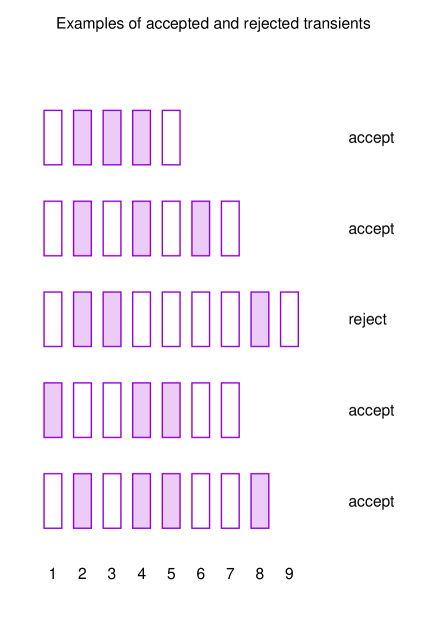
   Figure 4: Examples of sequences of images with detections (filled rectangles) and non-detections (empty rectangles), and our algorithm’s decision at right.

3. the magnitude of a candidate must be less than $(m+1)$, where $m$ is the limiting magnitude of the chunk (which we will discuss below). In other words, the object may be slightly fainter, on average, than the limiting magnitude.

4. the object must be at least 7 pixels ($8\hbox to0.0pt{.\hss}{{}^{\prime\prime}}3$) from its nearest neighbor in the ensemble. This rule rejects many bogus candidates in the outer regions of bright stars.

5. the object must be at least 10 pixels ($11\hbox to0.0pt{.\hss}{{}^{\prime\prime}}8$) from the edges of the image. Our routines for measuring accurately the properties of an object set this limit.

Conditions 1 and 2 can cause a real, very brief transient to be missed. If an object appears for exactly 3 images (1.5 seconds), and one of those images happens to be either the first or last frame in a chunk, or if it appears for exactly 4 images (2 seconds), and two of those happen to be the first two or last two of a chunk, then it will not pass the tests. Since this applies only to a very small fraction of all possible transients (about $0.6\%$ of those lasting with exactly 3 or 4 detections), we accept the losses.

Condition 5 causes us to ignore a thin strip around the edges of each image, amounting to $2.7\%$ of the area of the survey. We will account for this small inefficiency in our calculations of the control time and transient rates later in this paper.

Describing the “limiting magnitude” for an instrument can be approached in several ways. For example, under optimal conditions, a star of magnitude $V=18.5$ produces a signal-to-noise ratio of 5 in 1-second exposure with Tomo-e (Sako et al., 2018); so one might say that the 0.5-second exposures we studied ought to have a limiting magnitude of $V=17.7$ However, since our search was often conducted in less than optimal conditions, we take a more conservative approach in this paper. In order to calculate the limiting magnitude for a chunk, we begin by counting the number $N$ of “good” images with in the chunk. This is normally close to 360, but may be smaller if some frames are rendered unusable by clouds, bad seeing, passing airplanes, or other problems. We then compare the number of images in which each star is detected to $N$. Bright stars will appear in nearly all of them, but very faint stars may rise above the noise threshold only in a few images. We define the “limiting magnitude” of a chunk to be the magnitude at which the average number of detections falls to $N/2$. We record this limiting magnitude for each chunk, and use it not only to test possible transients, but also to compute control times (see section 5).

After running all the star lists through these tests, we found a total of 57 candidate transient objects. We examined each candidate in detail, scrutinizing the images before, during, and after its detections. We discovered that most of these candidates were simply ordinary stars, somewhat fainter than the limiting magnitude of our observations. Due to fortuitous moments of good seeing, they would sometimes pop up above the detection limit for a few consecutive frames before disappearing below the sky noise again. Although our software failed to notice them most of the time, a human eye could often detect them, once their positions were known. We examined 2MASS and Digitized Sky Survey images at the positions of all candidates to look for faint stars, and rejected all candidates with counterparts in these surveys. One example of this sort of object is shown in Figure 5.

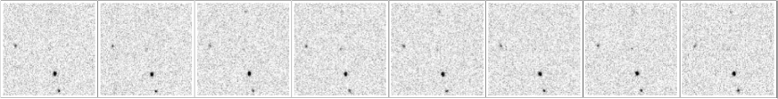
Figure 5: Cutouts centered on a candidate of March 30, 2016. The object was detected in the second, fourth, and seventh images in this sequence, but is present in all of them. Each cutout is 130 arcseconds on a side, with North up, East left. Time runs from left to right.

A few of the candidates were bright stars, far above the detection limit, which appeared offset from their usual positions due to particularly bad seeing. Short-term atmospheric fluctuations can lead to unusually distorted point spread functions when one integrates for very short durations. An example of this type of candidate is shown in Figure 6.

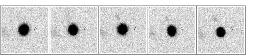
Figure 6: Cutouts centered on a candidate of Apr 11, 2016, during conditions of poor seeing. The software determined a position for this object in the central 3 images which was sufficiently offset from the usual position that it appeared as a new object. The red circle indicates the size of matching radius. Each cutout is 130 arcseconds on a side, with North up, East left. Time runs from left to right.

The most promising candidates appeared on the night of 2016 March 17, near RA $=169.24$ and Dec $=0.97$. Two of the seven candidates for this night turned out to be the same object, which was moving at a rate of about $5^{{}^{\prime\prime}}$ per second to the East. It was below the threshold of detection for most of the observations, but rose above the threshold for a few seconds and was detected twice, separated by a few seconds. Figure 7 shows subframes of consecutive images, centered on the candidate. The top row shows the first detection, and the lower row the second detection.

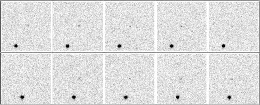
Figure 7: Cutouts centered on the moving candidate from March 17, 2016. Each cutout is 130 arcseconds on a side, with North up, East left. Time runs from left to right in each row.

Using tools provided by the Minor Planet Center, we found no known asteroids at this position. The motion is consistent with that of an artificial satellite in high-Earth orbit. When we examined the intervening images, we were able to detect it in most of them – but at a significance level below that required to trigger our star-finding routines.

In summary, we found zero stationary objects which appeared, and then disappeared, over a span of time between 1.5 and 11.5 seconds. However, the fact that our procedure did uncover a very faint, moving satellite, at two locations along its orbit, gives us some confidence that it would have flagged a real transient source as well.

What can we learn from this null result?

5 The rate of transient events

Following methods used by supernova researchers starting with Zwicky (1938), we introduce the concept of control time: the time during which a transient event would have been detected by our system, should it have occurred. In the case of supernovae, which remain bright for many weeks, one must take into account the possibility of an explosion happening some time before the start of an observation. Since we are interested in objects which fade only a few seconds after their rise, however, an interval much shorter than the duration of our measurements each night, our control time is simply the sum of our exposure times (after removing periods ruined by clouds, bad seeing, and other problems).

In the decades following Zwicky (1938), survey images typically covered the entire extent of some particular galaxy (and of many galaxies, in fact). Any supernova in that galaxy would appear in each survey image, and so the control time for that galaxy would be simply a function of the duration of the survey and the intervals between images. In most modern searches, including ours, which are not confined to some known and finite source, the control time must include a factor in addition to time: the area over which new objects could be detected. Clearly, for example, an eight-hour sequence of images covering ten square degrees provides more information than an eight-hour sequence of images reaching the same depth, but covering only one square degree. This example makes clear that another variable we must consider is the depth of the survey: an eight-hour sequence of images reaching $V=15$ provides more information than a similar sequence of images which reaches only $V=10$.

In order to characterize our survey for transients, therefore, we must describe

• the area of the sky covered; we will use square degrees

• the time span of the observations; we choose seconds

• the depth of the survey; see discussion below

In most circumstances, astronomers would describe the depth of a survey by its limiting magnitude, or limiting flux; these are appropriate choices to describe sources which are constant in brightness. Since we are searching for objects which might change in brightness considerably from one image to the next, however, or even during the exposure of a single image, it makes more sense to consider the concept of fluence. Fluence is the integral of flux over time; it might be the number of photons collected during one exposure, for example, or summed over several exposures.

Since our search criteria require that an object be detected in a series of (nearly) consecutive images, we can compute a rough lower limit on the fluence of an object that our algorithm would find:

$${\rm Fluence\ limit\ F\ }=10^{-0.4m}\thinspace ftN$$

where $m$ is the ordinary limiting magnitude of a single image, $f$ is the flux density corresponding to an object of magnitude zero, $t=0.5$ seconds is the exposure time of one of our images, and $N=3$ is the minimum number of consecutive images in which an object must appear. We adopt a value of $f=3.16\times 10^{-6}\thinspace{\rm erg/cm^{2}s}$, corresponding to the $V$-band zeropoint.

As described in the previous section, our pipeline computes a limiting magnitude $m$ for each chunk of images. We apply that value to all the images in a chunk in order to compute control times. Thus, we can not account properly for any changes in sky conditions on timescales shorter than the duration of a chunk (180 seconds).

Even though fluence is a better choice when describing the behavior of very brief transients, most of the literature on surveys for supernova, gamma-ray bursts, and other variable objects characterizes their measurements in terms of a limiting magnitude. In order to compare our results more easily with others, we will convert our results into those terms. Since we are looking for objects with lifetimes of just a few seconds, it is convenient to describe our results in terms of the fluence over a period of one second, or, equivalently, the limiting magnitude in a 1-second exposure. Since the conditions changed significantly within some nights, as well as from night to night, and since the properties of the sources which might appear in our data have very broad ranges, we have chosen to compute control times for a range of observed fluences, rather than a single value. We compute control times for four choices of this parameter, corresponding to limiting magnitudes of $V=12.6,\ 13.6,\ 14.6,{\rm\ and\ }15.6$, in a one-second exposure.‘ The results are presented in Table 2. The small value in the final entry for 2016 Apr 14 is due to a combination of bad seeing and clouds.

Table 2: Control time (sq.deg.*sec) for several thresholds

Date	$V=12.6$	$V=13.6$	$V=14.6$	$V=15.6$
2016 March 15	49,357	49,357	49,357	43,685
2016 March 16	40,520	40,520	38,834	33,083
2016 March 17	43,984	43,741	41,077	32,671
2016 March 30	30,133	29,292	25,108	19,253
2016 Apr 08	33,068	31,919	28,311	23,028
2016 Apr 09	30,015	29,298	25,848	10,807
2016 Apr 11	36,771	34,252	28,888	14,843
2016 Apr 14	28,216	25,715	20,015	128
total	292,069	284,100	257,441	177,502

Our goal is to use this information to determine the rate at which transients appear, in units of objects per square degree per second. Since we detected no events, however, we cannot perform this calculation in the simple way. Instead, we will use our measurements to place an upper limit on the rate at which transients appear. We will begin by making two assumptions:

1. transient events are independent of each other

2. the rate of events, $\lambda$, is constant during the course of our survey

With these assumptions, we can model the occurence of events as a Poisson distribution, so that the probability $p$ of $N$ events during some period $t$ is

$$p={{(\lambda t)^{N}\thinspace e^{-\lambda t}}\over{N!}}$$

We observed $N=0$ events. In order to place limits on the rate $\lambda$, we must choose some small probability $p_{0}$ that this lack of detections is due purely to chance. We make the arbitrary choice of $p_{0}=0.05$, and then reject any rate $\lambda$ which would yield a probability $p<p_{0}$ of observing zero events. This technique yields upper limits on the rate of transient events meeting our criteria, which we quote in units of events per square degree per day. These values are listed in Table 3 for the four choices of limiting fluence, and shown in Figure 8.

Table 3: Upper limit (95% confidence level) on rate (events per sq.deg. per day) for several thresholds

Fluence	$V=12.6$	$V=13.6$	$V=14.6$	$V=15.6$
Rate	$0.89$	$0.91$	$1.00$	$1.46$

Equivalent limiting mag in 1-sec exposure.

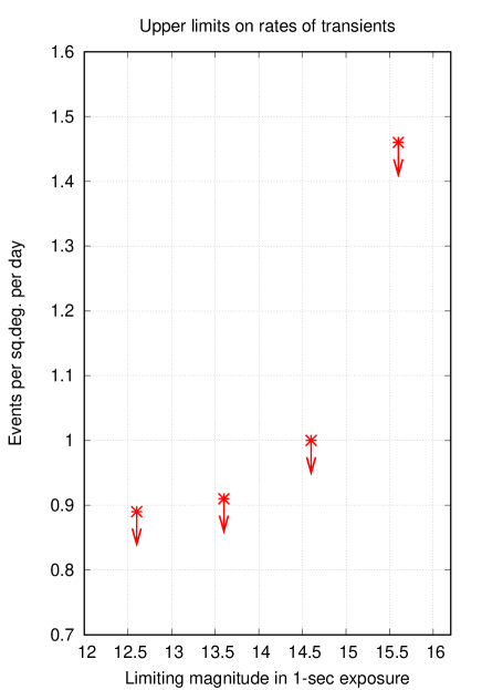
Figure 8: Upper limits to the areal rates of optical flashes

6 The volumetric rate of specific sources

If we know the properties of some specific type of brief-lived source, we can convert our limits from area-based (per square degree per second) to volume-based (per cubic pc per second). Let us assume that an explosion of some type produces a total energy $E$ in optical light over some short duration $\Delta t$ which lies within the range of our transient search. Assuming that the brightness of the source is roughly constant over this period, its flux $f$ will be

$$f={{E}\over{4\pi d^{2}}\thinspace\Delta t}$$

For any one of our chosen flux limits $f_{\rm lim}$ in Table 3, we can compute the maximum distance out to which such a source would be detected by our survey:

$$d_{\rm max}=\sqrt{{{E}\over{4\pi f_{\rm lim}\thinspace\Delta t}}}$$

To illustrate the method, we choose two representive sources: a “nearby” type, the impact of a small body onto a white dwarf, and a “distant” variety, the prompt optical flash of a gamma-ray burst. Our goal in the following discussion is to show the steps one can follow to compute volumetric rates from our survey’s data.

6.1 Asteroids and comets falling onto white dwarfs

The collision of small bodies onto the surface of a white dwarf is discussed in Di Stefano et al. (2015), and one sees evidence for it in the abundance of some heavy elements in the spectra of certain white dwarfs. The energy produced in the collision is released over a period which increases with the mass of the impactor. For objects of mass $m\sim 10^{14}$ g, Di Stefano et al. (2015) estimate that the optical flash might last for $\Delta t\sim 1$ second, and contain roughly $E\sim 10^{31}$ ergs. Using these values, we compute distances out to which such collisions would be detected, and list them in Table 4.

Table 4: Detection limit $d_{\rm max}$ for $10^{31}$ erg/s comet-WD collision

source	$V=12.6$	$V=13.6$	$V=14.6$	$V=15.6$
comet-WD	54 pc	86 pc	136 pc	215 pc

Once we know the distance $d_{\rm max}$ out to which a source could be detected, we can compute the effective volume for that type of source covered by of our survey. Let us perform one such calculation here as an example. For a fluence limit of $V=13.6$ mag in a 1-second exposure, we could detect a comet-WD collision out to a distance of $d_{\rm max}=86$ pc. Since our rates listed in Table 3 have units of “per square degree,” the effective volume of our search will be that of a narrow spherical sector with radius $d_{\rm max}$. The ratio of the volume of this sector to the volume of a full sphere will be the ratio of the area of one square degree to the area of a full sphere; thus,

$${\rm effective\ volume\ }V_{\rm eff}\quad=\quad{{4\pi}\over{3}}(d_{\rm max})^{3}\thinspace\left({{1{\rm\ sq.\ deg.}}\over{4\pi\ {\rm ster}}}\right)\quad=\quad 2.42\times 10^{-5}\thinspace{{4\pi}\over{3}}(d_{\rm max})^{3}$$

In our example, since $d_{\rm max}=86$ pc, the effective volume is $V_{\rm eff}=64.6$ cubic pc. Multiplying this volume by the duration portion of the control time will yield a “control volume:” in this case, 64.6 (cubic pc $\times$ day). In a similar way, we can convert our upper limit on the rate of transients from areal to volumetric by dividing the rate in Table 3 by this effective volume. For our example,

$${\rm volumetric\ rate\ }r_{\rm vol}\quad\leq\quad{{0.91\thinspace{\rm events/sq.deg.\cdot day}}\over{64.6\thinspace{\rm pc}^{-3}/{\rm sq.deg.}}}\quad=\quad 1.4\times 10^{-2}\thinspace{\rm events}/{\rm pc^{-3}\cdot day}$$

Di Stefano et al. (2015) estimate that the number of comet-WD collisions in a typical galaxy is $8\times 10^{6}$ per year. If we model the disk of the Milky Way as a thin disk of radius $10$ kpc and height $1$ kpc, its volume is $3\times 10^{11}\ {\rm pc^{3}}$; our upper limit to the rate (for a fluence equivalent to $V=15.6$ in a 1-second exposure) would imply that no more than $\sim 1.6\times 10^{11}$ events should occur within the entire galaxy each year. While this is certainly consistent with the expections of Di Stefano et al. (2015), it is far from being a strict constraint.

6.2 Prompt optical flashes of gamma-ray bursts

In many cases, optical emission has been detected hours to days after a GRB, as part of the physical process called the afterglow. In a very few cases, optical telescopes have seen flashes at the same time as the initial burst of gamma rays. We will take as models three events in which the optical flash was particular bright: GRBs 080319B (Racusin et al., 2008; Covino et al., 2008; Woźniak et al., 2009), 130427A (Tanvir et al., 2013; Vestrand et al., 2014), and 160625B (Batsch et al., 2016; Troja et al., 2017; Karpov et al., 2017). All three are classified as “long” GRBs, as instruments detected gamma rays from them for durations longer than two seconds (see Berger (2014) and Pe’er (2015) for reviews of GRB properties). In each of these cases, the GRB seems to have been caused by the collapse of a massive star.

The calculations of $d_{\rm max}$ and volumetric rate for these very luminous and distant events are more complicated than those for “nearby” objects for two reasons. First, the relationship between distance and apparent brightness is not the simple Euclidean $1/r^{2}$, due to the curvature of space-time and relativistic effects. Second, when determining the observed properties of objects at redshifts $z>0.5$, one must account for the difference between the spectral region in which light was emitted in the rest frame, and the spectral region in which the light is detected by the observer; in other words, one must know the shape of the source’s spectral energy distribution.

Based on the optical and gamma-ray observations of the 3 model GRBs in our comparison set, we have constructed a “toy model” of the prompt emission from such an event: a simple power-law spectrum with a cutoff at $h\nu_{0}=2000$ keV.

$${\rm flux\ density\ }f_{\nu}=\left\{\begin{array}[]{ll}A\thinspace{\left({{\nu}\over{\nu_{0}}}\right)}^{-0.5}&\nu\leq\nu_{0}\\ 0&\nu>\nu_{0}\\ \end{array}\right.$$

The amplitude $A$ is proportional to the overall luminosity of prompt emission. We choose to describe it by computing an “overall gamma-ray peak luminosity,” $L_{\gamma}$, for the flash, which we calculate using rest-frame emission in the range $10-2000$ keV. For a wide range of such luminosities, we then determine the redshifts at which our model’s observed optical brightness would fall below our four limiting magnitudes; the results are shown in Figure 9. Note that the intergalactic medium is likely to be ionized at $z\gtrsim 5.5$ (Songaila, 2004), and hence opaque to the (at that time) ultraviolet photons flying toward us. However, it is possible that some windows of low opacity might allow the detection of a small fraction of sources beyond this redshift.

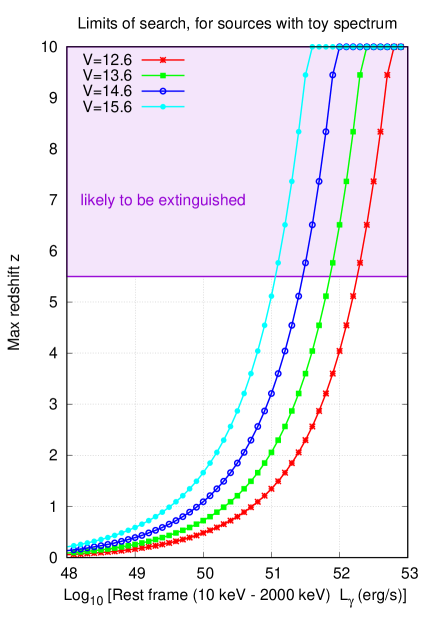
Figure 9: Upper limits to the redshifts at which our survey could detect prompt optical flashes from GRBs.

When we set the value of $A$ so that the model optimally matches the gamma-ray and optical observations of the three comparison events (to within an order of magnitude in all cases), we derive a value of $L_{\gamma}=6\times 10^{52}$ erg/s. This implies that events similar to those in the comparison set would be detected to redshifts $z>9$ even for our brightest choice of magnitude limit.

Given a redshift, one can compute the comoving volume within a spherical region and convert the areal rates listed in Table 3 into volumetric form. These rates, in units of events per cubic Gpc per year, are displayed in Figure 10. We arbitrarily set an upper limit of $z=10$ for the explosion of GRBs, causing the rates to reach fixed values at high luminosities, when the flashes can be seen throughout the entire volume. We list those fixed rates in Table 5. Note that when the search can detect events anywhere in the volume, the rate for particular limiting magnitude depends solely on the control time; thus, the case of $V=15.6$ ceases to provide the most stringent upper limit because its control time was smaller than that of $V=14.6$ or $V=13.6$.

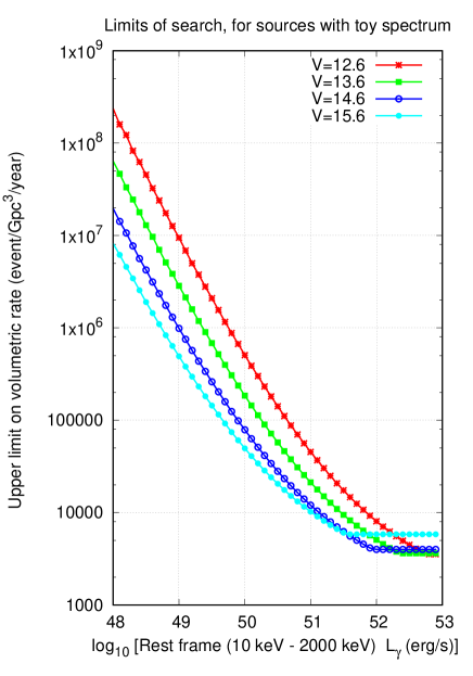
Figure 10: Upper limits to the volumetric rates of GRBs with bright prompt optical flashes.

Table 5: Upper limits (95% confidence level) for rates of very luminous sources

	$V=12.6$	$V=13.6$	$V=14.6$	$V=15.6$
if $L_{\gamma}$ (erg/s) is greater than	$6.3\times 10^{52}$	$2.5\times 10^{52}$	$1.0\times 10^{52}$	$4.0\times 10^{51}$
then rate (${\rm Gpc^{-3}\thinspace yr^{-1}}$) is less than	$3600$	$3700$	$4000$	$5800$

Let us briefly consider one implication of these calculations. While the particular GRBs upon which our model was created are due to events within the core of a massive star, the separate class of short GRBs is thought to be due, in part at least, to the mergers of binary neutron stars (NS). The rate of NS-NS mergers has become a hot topic of late, thanks to the success of LIGO and Virgo. Chruslinska (2018) provides a nice summary of both observational measurements of the rate, and theoretical expectations based on population synthesis and binary evolution. The observations suggest somewhat higher rates than the models, with some estimates reaching a few thousand per ${\rm Gpc^{3}}$ per year. If (and we stress that this is a big qualification) the NS-NS merger mechanism should produce a prompt spectrum similar to that of the long GRBs in our comparison set, then continuing a search like ours for several months or years could place meaningful constraints on the rates of such mergers.

7 Comparison with other transient searches

Many groups have examined the sky for ephemeral sources over the past century, but the great majority considered timescales much longer than the range of 1.5 - 11.5 seconds that we explore in this work. For example, the Deep Lens Survey Transient Search (Becker et al., 2004), and efforts using data from ROTSE-III (Rykoff et al., 2005), MASTER (Lipunov et al., 2007), DECam (Andreoni et al., 2019), and PanSTARRS (Berger et al., 2013) all required a source to remain bright for long enough to appear in at least two images of moderate to long exposure time, leading to minimum durations of hundreds or thousands of seconds. Because all these projects could detect sources much fainter than Tomo-e PM, the control volumes they examined were three to five orders of magnitude greater than that described in this work. However, since the transients we seek herein would appear in only a single exposure of all those projects, and so be discarded, there seems little reason to consider them further.

Instead, let us compare our survey briefly with three other projects which are sensitive to transients within our chosen timescale and appear to be ongoing: Pi of the Sky, Mini-Mega-TORTORA, and Gaia.

Pi of the Sky (Sokolowski, 2008; Obara et al., 2014) consists of one system in Atacama, Chile, with two cameras, and three systems in INTA, Spain, with four cameras each. Each camera consists of a 85-mm f/1.2 camera lens which focuses light onto a CCD, yielding a field of $20^{\circ}\times 20^{\circ}$ with pixels subtending $36^{{}^{\prime\prime}}$ on a side. Exposures of length 10 seconds detect objects down to $V\sim 12$; this corresponds to a limit of about $V\sim 9.5$ in a 1-second exposure. The weather at all sites is very good, providing images of very large areas of the sky on many nights per year.

Mini-Mega-TORTORA, hereafter denoted MMT-9 (Karpov et al., 2016), is based at the Special Astrophysical Observatory in the Caucasus, where the sky is somewhat cloudy. Nine independent units, each built around an 85-mm f/1.2 camera lens and Andor Neo CMOS detector, provide images covering $9^{\circ}\times 11^{\circ}$ with pixels subtending $16^{{}^{\prime\prime}}$ on a side. Images with exposure times of 0.128 seconds are taken 7.5 times per second, providing very high time resolution. The limiting magnitude in a single exposure is $V\sim 11$, corresponding to a 1-second limit of $V\sim 13.3$.

The Gaia spacecraft rotates on its axis with a period 108 minutes, causing objects to drift across its focal plane. (Wevers et al., 2018) describe a technique for examining the measurements from individual chips, yielding sets of 11 exposures, each 4.5 seconds in length, covering a span of 45 - 50 seconds. Stars to $G\sim 20.5$ can be detected in each chip, equivalent to $V\sim 19.0$ in a 1-second exposure. Over the course of one day, the spacecraft will scan roughly 1000 square degrees of the sky. Due to the way in which objects are detected and followed across the Gaia focal plane, transients with the very short durations (1.5 - 11.5 seconds) we consider in this paper will be detected with a low efficiency ($\sim 0.1$) and appear in at most two of the nine Astrometric Field chips. Transients of this sort were not included in the analysis of Wevers et al. (2018), nor do they appear in Gaia DR2, but it is possible that researchers might make special efforts to identify them in the low-level data products.

How do these projects compare to Tomo-e for finding transients with durations of order one second? We will compute a statistic, “relative control volume (RCV),” which accounts for the properties of each survey, yielding a relative measure of the volume monitored per day; larger values of RCV correspond to more frequent observations of transient objects, and thus more stringent limits on their rates. We use a simple Euclidean model in these calculations.

$${\rm RCV}=\left({{\rm hours\ active}\over{\rm day}}\right)\left({{\rm sq.deg.}\over{\rm hour}}\right)\left(d_{\rm max}^{\thinspace 3}\right)$$

The depth $d_{\rm max}$ of each survey is measured relative to that of Tomo-e PM, based on the limiting magnitude for an equivalent 1-second exposure. We have estimated an average duration of 8 hours per night for the ground-based instruments, and have assumed that both Pi of the Sky and MMT-9 are configured for maximum sky coverage. We have multiplied the “area scanned per hour” entry for Gaia by $0.1$ to account for its low efficiency of detecting very brief transients.

Table 6: Comparison of some active survey instruments

	${\rm Tomo-ePM}$	${\rm Tomo-e}$	${\rm PiSky}$	${\rm MMT-9}$	${\rm Gaia}$
Hours per day	$8$	$8$	$8$	$8$	$24$
Area per hour (sq.deg)	$1.9$	$20.4$	$6400$	$6900$	$3.9$
Pixel size (arcsec)	$1.2$	$1.2$	$36$	$16$	$0.18$
Lim. mag in image	$17.8/14.9$	$17.8/14.9$	$12$	$11$	$20.6$
Time resolution (s)	$0.5$	$0.5$	$10$	$0.12$	$4.5$
Lim. mag in 1-sec	$18.5/15.6$	$18.5/15.6$	$9.5$	$13.3$	$19.0$
Normalized $d_{\rm max}$	$1.0$	$1.0$	$0.060$	$0.42$	$4.8$
RCV	$15.2$	$163$	$11$	$2300$	$10,000$

For Tomo-e, first value under optimal conditions; second value faintest limit used in control time calculations

The Tomo-e PM system appears comparable to the Pi of the Sky by this metric, and far below the MMT-9 and Gaia instruments. Observations by the full Tomo-e system, which have recently started at the time of writing (June 2019), will increase its RCV by roughly a factor of ten, simply by increasing the number of CMOS sensors from 8 to 84; this increase places Tomo-e roughly halfway between Pi of the Sky and MMT-9, in a logarithmic sense.

Of course, this metric is not the only way to evaluate the performance of any of these surveys. Each has its own strengths and weaknesses, and each can and does provide valuable information to those interested in transient events. One of Tomo-e’s strengths is its relatively high angular resolution and uniform PSF across the field of view: it suffers less from crowding and image distortions than Pi of the Sky and MMT-9, which may allow it to make more accurate measurements of some events, or even to detect some marginal events which might appear blended in other systems. On the other hand, its location in the mountains of central Japan, while providing a dark sky, also delivers cloudy weather more frequently than the sites of Pi of the Sky and Gaia.

8 Funding

Our studies are supported in part by the Japan Society for the Promotion of Science (JSPS) Grants-in-Aid for Scientific Research (KAKENHI) Grant Number JP25103502, JP26247074, JP24103001, JP16H02158, JP16H06341, JP2905, 18H04575, JP18H01272, JP18H01261, and JP18K13599. This research is also supported in part by the Japan Science and Technology (JST) Agency’s Precursory Research for Embryonic Science and Technology (PRESTO), the Research Center for the Early Universe (RESCEU), of the School of Science at the University of Tokyo, and the Optical and Near-infrared Astronomy Inter-University Cooperation Program.

This research has made use of NASA’s Astrophysics Data System. We thank the Minor Planet Center for providing the Minor Planet Checker and NEO Checker services to the community. Ned Wright’s cosmological calculator (Wright, 2006) was a great aid in our work.

References

- Abbott et al. (2017) Abbott, B. P., Abbott, R., Abbott, T. D., et al. 2017, Physical Review Letters, 119, 161101
- Andreoni et al. (2019) Andreoni, I., Cooke, J., Webb, S., et al. 2019, arXiv:1903.11083
- Becker et al. (2004) Becker, A. C., Wittman, D. M., Boeshaar, P. C., et al. 2004, ApJ, 611, 418
- Berger et al. (2013) Berger, E., Leibler, C. N., Chornock, R., et al. 2013, ApJ, 779, 18
- Berger (2014) Berger, E. 2014, ARA&A, 52, 43
- Batsch et al. (2016) Batsch, T., Castro-Tirado, A. J., Czyrkowski, H., et al. 2016, GRB Coordinates Network, Circular Service, No. 19615, #1 (2016), 19615, 1
- Chruslinska (2018) Chruslinska, M. 2018, arXiv e-prints , arXiv:1811.09296.
- Covino et al. (2008) Covino, S., Guidorzi, C., Margutti, R., et al. 2008, American Institute of Physics Conference Series, 1059, 59
- Di Stefano et al. (2015) Di Stefano, R., Fisher, R., Guillochon, J., & Steiner, J. F. 2015, arXiv:1501.07837
- Honeycutt (1992) Honeycutt, R. K. 1992, PASP, 104, 435
- Karpov et al. (2016) Karpov, S., Beskin, G., Biryukov, A., et al. 2016, Revista Mexicana de Astronomia y Astrofisica Conference Series, 48, 91
- Karpov et al. (2017) Karpov, S., Beskin, G., Biryukov, A., et al. 2017, Stars: From Collapse to Collapse, 510, 309
- Lipunov et al. (2007) Lipunov, V. M., Kornilov, V. G., Krylov, A. V., et al. 2007, Astronomy Reports, 51, 1004
- Obara et al. (2014) Obara, L., Cwiek, A., Cwiok, M., et al. 2014, Revista Mexicana de Astronomia y Astrofisica Conference Series, 45, 118
- Ohsawa et al. (2016) Ohsawa, R., Sako, S., Takahashi, H., et al. 2016, Software and Cyberinfrastructure for Astronomy IV, 991339
- Pe’er (2015) Pe’er, A. 2015, Advances in Astronomy, 2015, 907321
- Racusin et al. (2008) Racusin, J. L., Karpov, S. V., Sokolowski, M., et al. 2008, Nature, 455, 183
- Richmond (2017) Richmond, M. W. 2017, http://spiff.rit.edu/tass/xvista
- Rykoff et al. (2005) Rykoff, E. S., Aharonian, F., Akerlof, C. W., et al. 2005, ApJ, 631, 1032
- Sako et al. (2016) Sako, S., Osawa, R., Takahashi, H., et al. 2016, Proc. SPIE, 9908, 99083P
- Sako et al. (2018) Sako, S., Ohsawa, R., Takahashi, H., et al. 2018, Ground-based and Airborne Instrumentation for Astronomy VII, 10702, 107020J
- Siellez et al. (2016) Siellez, K., Boer, M., Gendre, B., & Regimbau, T. 2016, arXiv:1606.03043
- Sokolowski (2008) Sokolowski, M. 2008, Ph.D. Thesis
- Songaila (2004) Songaila, A. 2004, AJ, 127, 2598
- Tanvir et al. (2013) Tanvir, N. R., Levan, A. J., Fruchter, A. S., et al. 2013, Nature, 500, 547
- Troja et al. (2017) Troja, E., Lipunov, V. M., Mundell, C. G., et al. 2017, Nature, 547, 425
- Treffers & Richmond (1989) Treffers, R. R., & Richmond, M. W. 1989, PASP, 101, 725
- Vestrand et al. (2014) Vestrand, W. T., Wren, J. A., Panaitescu, A., et al. 2014, Science, 343, 38
- Wevers et al. (2018) Wevers, T., Jonker, P. G., Hodgkin, S. T., et al. 2018, MNRAS, 473, 3854
- Woźniak et al. (2009) Woźniak, P. R., Vestrand, W. T., Panaitescu, A. D., et al. 2009, ApJ, 691, 495
- Wright (2006) Wright, E. L. 2006, PASP, 118, 1711
- Zacharias et al. (2013) Zacharias, N., Finch, C. T., Girard, T. M., et al. 2013, AJ, 145, 44
- Zwicky (1938) Zwicky, F. 1938, ApJ, 88, 529