Case Study: Verifying the Safety of an Autonomous Racing Car with a Neural Network Controller

Abstract.

This paper describes a verification case study on an autonomous racing car with a neural network (NN) controller. Although several verification approaches have been proposed over the last year, they have only been evaluated on low-dimensional systems or systems with constrained environments. To explore the limits of existing approaches, we present a challenging benchmark in which the NN takes raw LiDAR measurements as input and outputs steering for the car. We train a dozen NNs using two reinforcement learning algorithms and show that the state of the art in verification can handle systems with around 40 LiDAR rays, well short of a typical LiDAR scan with 1081 rays. Furthermore, we perform real experiments to investigate the benefits and limitations of verification with respect to the sim2real gap, i.e., the difference between a system’s modeled and real performance. We identify cases, similar to the modeled environment, in which verification is strongly correlated with safe behavior. Finally, we illustrate LiDAR fault patterns that can be used to develop robust and safe reinforcement learning algorithms.

1. Introduction

Neural networks (NNs) have shown great promise in multiple application domains, including safety-critical systems such as autonomous driving (Bojarski et al., 2016) and air traffic collision avoidance systems (Julian et al., 2016). At the same time, widespread adoption of NN-based autonomous systems is hindered by the fact that NNs often fail in seemingly unpredictable ways: slight perturbations in their inputs can result in drastically different outputs, as is the case with adversarial examples (Szegedy et al., 2013). Such issues might lead to fatal outcomes in safety-critical systems (Board, [n.d.]) and thus underscore the need to assure the safety of NN-based systems before they can be deployed at scale.

One way to reason about the safety of such systems is to formally verify safety properties of a NN’s outputs for certain sensitive inputs, as proposed in several NN verification and robustness works (Dutta et al., 2018; Ehlers, 2017; Katz et al., 2017; Wang et al., 2018; Weng et al., 2018). However, safety of the NN does not immediately imply safety of the entire autonomous system. A more exhaustive approach is to consider the interaction between the NN and the physical plant (e.g., a car), trace the evolution of the plant’s states (e.g., position, velocity) over time and ensure all reachable states are safe. A few such methods were recently developed to verify safety of autonomous systems with NN controllers (Dutta et al., 2019; Ivanov et al., 2019; Sun et al., 2019; Tran et al., 2019). These techniques combine ideas from classical dynamical system reachability (Chen et al., 2013; Kong et al., 2015; Tran et al., 2019) (e.g., view the NN as a hybrid system) with NN verification approaches (e.g., cast NN verification as a mixed integer linear program). However, these approaches have so far been evaluated on fairly simple systems: either systems with low-dimensional NN inputs (the inputs are the plant states, e.g., position and velocity (Dutta et al., 2019; Ivanov et al., 2019; Tran et al., 2019)) or with constrained environments (e.g., LiDAR orientation does not change over time (Sun et al., 2019)).

Two main challenges remain in applying verification techniques to realistic systems. The first one is scalability. There are (at least) two aspects to this challenge: 1) scalability with respect to (w.r.t) the plant dynamics and 2) and scalability w.r.t. the NN complexity. The reachability problem is undecidable for general hybrid systems (Alur et al., 1995), which means existing approaches can only approximate the reachable sets. The NN adds additional complexity both due to size and due to the number of inputs to the NN – it is much more challenging to compute reachable sets for multivariate functions, even for small NNs. At the same time, having the capability to verify systems with high-dimensional measurements is crucial, since NNs are most useful exactly in such settings.

The second verification challenge is the sim2real gap, i.e., the difference between a system’s modeled and real performance (Chebotar et al., 2019). Analyzing the sim2real gap is essential as it allows us to explore the benefit of verification with the respect to the real system. Overcoming this challenge would enable developers to design and test approaches in simulation with the assurance that safety properties that hold in simulation would carry over to the real world.

In order to illustrate these difficulties and to provide a challenging benchmark for future work, this paper presents a verification case study on a realistic NN-controlled autonomous system. In particular, we focus on the F1/10 autonomous racing car (f1t, [n.d.]), which needs to navigate a structured environment using high-dimensional LiDAR measurements. This case study has two goals: 1) assess the capabilities of existing verification approaches and highlight aspects that require future work; 2) investigate conditions under which the verification translates to safe performance in the real world.

To perform the verification, we first identify a dynamics (bicycle) model of the F1/10 car, as well as an observation model mapping the vehicle state to the LiDAR measurements. To obtain the observation model, we assume the car operates in a structured environment (i.e., a sequence of hallways) such that each LiDAR ray can be calculated based on the car’s state and the surrounding walls. Given these models, we train an end-to-end NN controller using reinforcement learning (Lillicrap et al., 2015). The controller takes LiDAR measurements as input and produces steering commands as output (assuming constant throttle). Once the NN is trained, we aim to verify that the car does not crash in the hallway walls.

We evaluate the scalability of existing verification approaches by varying the NN size, the number of LiDAR rays as well as the training algorithm. Note that the complexity of the verification task grows exponentially with the number of rays since, depending on the uncertainty, a given ray could reach different walls, which triggers multiple paths in the hybrid observation model that need to be verified simultaneously. We use the state-of-the-art tool Verisig (Ivanov et al., 2019) to verify the dozen setups that were trained; we could not encode the hybrid LiDAR model in the other existing tools. In our evaluation, Verisig could handle NNs of roughly 250 neurons (containing two layers with 128 neurons each) and LiDAR scans with around 40 rays. This highlights the challenge of this verification task: verifying the entire LiDAR scan containing 1081 rays, together with a corresponding NN that can effectively process such a scan, remains well beyond the capabilities of existing tools.

Finally, we perform experiments, using the verified controllers, to evaluate the system’s sim2real gap. This gap is especially pronounced with LiDAR measurements, since rays can get reflected depending on the reached surface, thereby providing an erroneous distance. We first evaluate the benefit of verification in an ideal setting by performing experiments with all reflective surfaces covered – all NNs performed similarly in this setup, resulting in safe behavior roughly 90% of the time; even in these cases crashes were caused by LiDAR faults that could not be completely eliminated. However, more crashes were observed in the unmodified environment, as caused by consistently bad LiDAR data. Upon closer investigation, we identified patterns of LiDAR faults that reproduce the unsafe behavior in simulations as well – however, we could not train a robust controller using the state-of-the-art reinforcement learning algorithms. Thus, it remains an open problem to train (and verify) a NN that provides safe performance in the presence of LiDAR errors.

In summary, this paper has three contributions: 1) a challenging benchmark for verification and reinforcement learning in neural-network-controlled autonomous systems with high-dimensional measurements; 2) an exhaustive evaluation of a state-of-the-art verification tool on this benchmark; 3) real experiments that illustrate the benefits and limitations of verification w.r.t. the sim2real gap.

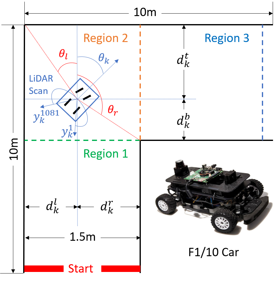
Figure 1. Navigation scenario. There are three different regions depending on how many walls can be reached using LiDAR.

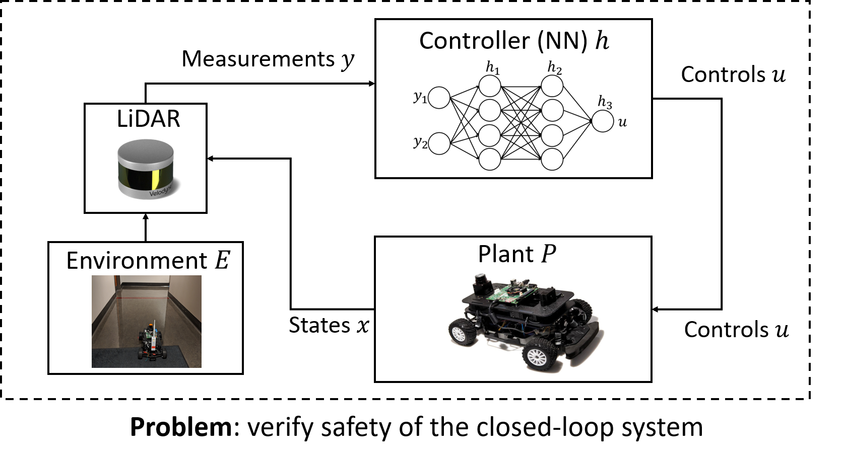
Figure 2. Overview of the closed-loop system and the problem considered in this paper.

2. System Overview

This section summarizes the different parts of the case study considered in the paper. We first describe the F1/10 platform, followed by a high-level introduction to reinforcement learning and hybrid system verification.

2.1. The F1/10 Autonomous Racing Car

The case study considered in this paper is inspired by the F1/10 Autonomous Racing Competition (f1t, [n.d.]), where an autonomous car must navigate a structured environment (i.e., the track) as fast as possible. The F1/10 car is shown in Figure 2. It is built for racing purposes and can reach up to 40mph. The car is controlled by an onboard chip such as the NVIDIA Jetson TX2 module.

A diagram of the closed-loop system is shown in Figure 2. The car operates in a hallway environment; without loss of generality, we assume that all turns are 90-degree right turns such that the “track” is effectively a square. Although in the competition the car has access to a number of sensors, in this case study we assume the controller only has access to LiDAR measurements. The measurements are sent to a NN controller that outputs a steering command to the vehicle. We assume that the car operates at constant throttle, in order to keep the dynamics model and the verification task manageable. The car’s dynamic and observation models used in the case study are described in Section 3.

2.2. Reinforcement Learning

Overall, developing a robust controller for the F1/10 car is a challenging task, both due to the difficulty of analyzing LiDAR measurements and to the speed and agility of the car. Thus, this is a good application for reinforcement learning (Lillicrap et al., 2015), where no knowledge of the car dynamics or the observation model is required. In reinforcement learning, the controller starts by applying a control action and observing a reward. As training proceeds, the learning problem is to maximize the reward by exploring the state space and trying different controls. In recent years, deep reinforcement learning (where controllers are neural networks) has shown great promise in a number of traditionally challenging problems, such as playing Atari games (Mnih et al., 2015), controlling autonomous cars (Bojarski et al., 2016) and playing board games (Silver et al., 2016). Hence, reinforcement learning is a natural choice for learning a controller for the F1/10 car as well; the specific training approach is described in Section 4.

2.3. Hybrid System and NN Verification

The hybrid system verification problem can be stated at a high level as follows: given a hybrid model of the plant dynamics and observations, the problem is to trace the evolution of the plant states over time (for a set of initial conditions) and verify that no unsafe states can be reached. Although hybrid system reachability is undecidable except for special cases such as linear systems (Alur et al., 1995; Lafferriere et al., 1999) (see (Alur, 2011; Doyen et al., 2018) for an exhaustive discussion), several approaches work well for specific non-linear systems. In particular, reachability is $\delta$-decidable for Type 2 computable functions (Kong et al., 2015), which has led to the development of the tool dReach. Alternatively, Flow* (Chen et al., 2013) constructs Taylor model (TM) approximations of the system’s reachable set. While Flow* provides no decidability claims, it can verify interesting properties for multiple non-linear systems classes and scales well when using TMs with interval analysis.

Recently, several approaches were developed for verification of hybrid systems with NNs controllers (Dutta et al., 2019; Ivanov et al., 2019; Sun et al., 2019; Tran et al., 2019). As described in Section 1, the NN introduces new challenges both due to its size and complexity. To address this issue, the proposed approaches borrow ideas from classical hybrid system reachability, e.g., by transforming the NN into a mixed-integer linear program (MILP) (Dutta et al., 2019), a satisfiability modulo theory (SMT) formula (Sun et al., 2019) or an equivalent hybrid system (Ivanov et al., 2019). Although existing tools have shown promising scalability in terms of the size of the NN, they have only been evaluated on low-dimensional systems or systems with constrained environments. In this paper, we provide a much more challenging scenario, with a high-dimensional hybrid observation model, in order to test the limits of these tools and to highlight avenues for future work.

2.4. System Design and Development

In order to build and verify the system, we perform the following steps: 1) build a model of the car dynamics and observations; 2) train a NN on the model using reinforcement learning; 3) verify that the NN-controlled car is safe with respect to the model; 4) perform real experiments to analyze the sim2real gap. The following sections describe each of these steps in more detail.

3. Plant Model

This section describes the F1/10 car’s dynamical and observation models. These models are used to train the NN controller (Section 4) and to perform the closed-loop system verification (Section 5).

3.1. Dynamics model

We use a bicycle model (Polack et al., 2017; Rajamani, 2011) to model the car’s dynamics, which is a standard model for cars with front steering. Specifically, we use a kinematic bicycle model since it has few parameters (that are easy to identify) and tracks reasonably well at low speeds, i.e., under 5 m/s (Rajamani, 2011). In the kinematic bicycle model, the car has four states: position in two dimensions, linear velocity and heading. The continuous-time dynamics are given by the following equations:

(1) $$\begin{split}\dot{x}&=vcos(\theta+\beta)\\ \dot{y}&=vsin(\theta+\beta)\\ \dot{v}&=-c_{a}v+c_{a}c_{m}(u-c_{h})\\ \dot{\theta}&=\frac{Vcos(\beta)}{l_{f}+l_{r}}tan(\delta)\\ \beta&=tan^{-1}\left(\frac{l_{r}tan(\delta)}{l_{f}+l_{r}}\right),\\ \end{split}$$

where $v$ is the car’s linear velocity, $\theta$ is the car’s orientation, $\beta$ is the car’s slip angle and $x$ and $y$ are the car’s position; $u$ is the throttle input, and $\delta$ is the heading input; $c_{a}$ is an acceleration constant, $c_{m}$ is a car motor constant, $c_{h}$ is a hysteresis constant, and $l_{f}$ and $l_{r}$ are the distances from the car’s center of mass to the front and rear, respectively. Since $tan^{-1}$ is not supported by most hybrid system verification tools, we assume that $\beta=0$; this is not a limiting assumption in the considered case study as the slip angle is typically fairly small at low speeds; we did not observe significant differences in the model’s predictive power due to this assumption. After performing system identification, we obtained the following parameter values: ${c_{a}=1.633},{c_{m}=0.2},{c_{h}=4},{l_{f}=0.225m},{l_{r}=0.225m}$. Finally, we assume a constant throttle $u=16$ (resulting in a top speed of roughly 2.4 m/s), i.e., the controller only controls heading. We emphasize that the plant model is fairly non-linear, thus making it difficult to compute reachable sets for the car’s states.

3.2. Observation model

The F1/10 car has access to LiDAR measurements only. As shown in Figure 2, a typical LiDAR scan consists of a number of rays emanating from -135 to 135 degrees relative to the car’s heading. For each ray, the car receives the distance to the first obstacle the ray hits; if there are no obstacles within the LiDAR range, the car receives the maximum range. In this case study, we consider a LiDAR scan with a maximum of 1081 rays and a range of 5 meters.

As shown in Figure 2, there are three possible regions the car can be in, depending on how many walls can be reached using LiDAR. The worst case is Region 2, in which there are four walls to consider. We present the measurement model for Region 2 only since the other regions are special cases of Region 2. Let $\alpha_{1},\dots,\alpha_{1081}$ denote the relative angles for each ray with respect to the car’s heading, i.e., $\alpha_{1}=-135,\alpha_{2}=-134.75,\dots,\alpha_{1081}=135$. One can determine which wall each LiDAR ray hits by comparing the $\alpha_{i}$ for that ray with the relative angles to the two corners of that turn, $\theta_{l}$ and $\theta_{r}$ in Figure 2. The measurement model for Region 2 (for a right turn) is presented below, for $i\in\{1,\dots,1081\}$:

(2) $$\begin{split}y_{k}^{i}=\left\{\begin{array}[]{lll}d^{r}_{k}/cos(90+\theta_{k}+\alpha_{i})&&\text{if }\theta_{k}+\alpha_{i}\leq\theta_{r}\\ d^{b}_{k}/cos(180+\theta_{k}+\alpha_{i})&&\text{if }\theta_{r}<\theta_{k}+\alpha_{i}\leq-90\\ d^{t}_{k}/cos(\theta_{k}+\alpha_{i})&&\text{if }-90<\theta_{k}+\alpha_{i}\leq\theta_{l}\\ d^{l}_{k}/cos(90-\theta_{k}-\alpha_{i})&&\text{if }\theta_{l}<\theta_{k}+\alpha_{i},\end{array}\right.\end{split}$$

where $k$ is the sampling step (the sampling rate is assumed to be 10Hz), $d^{t}_{k},d^{b}_{k},d^{l}_{k},d^{r}_{k}$ are distances to the four walls, as illustrated in Figure 2, and can be derived from the car’s position $(x,y)$. Similar to the dynamics model, the measurement model is non-linear. Furthermore, keeping the approximation error small during the reachability analysis is challenging since if a ray is almost parallel to a wall, small uncertainty in the car’s heading results in large uncertainty in the measured distance for that ray, which is evident in the division by cosine in the measurement model.

DRL algorithm	NN setup	# LiDAR rays	Controller index	Initial interval size	NN ver. time (s)	Total ver. time (s)	# paths
DDPG	$64\times 64$	21	1	0.2cm	355	4126	1.32
DDPG	$64\times 64$	21	2	0.2cm	347	4122	1.15
DDPG	$64\times 64$	21	3	DNF
DDPG	$128\times 128$	21	1	DNF
DDPG	$128\times 128$	21	2	DNF
DDPG	$128\times 128$	21	3	DNF
TD3	$64\times 64$	21	1	0.5cm	553	4731	2.2
TD3	$64\times 64$	21	2	0.5cm	853	8094	2.825
TD3	$64\times 64$	21	3	0.5cm	724	8641	2.725
TD3	$128\times 128$	21	1	0.5cm	197	3760	1.6
TD3	$128\times 128$	21	2	0.5cm	355	5954	1.775
TD3	$128\times 128$	21	3	Verisig/Flow* crash
TD3	$64\times 64$	41	1	0.2cm*	634	11915	2.194
TD3	$128\times 128$	41	1	DNF
TD3	$64\times 64$	61	1	DNF
TD3	$128\times 128$	61	1	DNF

Table 1. Verification evaluation for various setups in terms of NN architectures and number of LiDAR rays. The verification times and the number of paths are averaged over all subsets for each setup. Subset sizes are decreased from 0.5cm to 0.2cm and to 0.1cm, if verification fails. DNF setups were terminated after 10 hours on 0.1cm subsets. The notation $n\times n$ means that this is a NN with two hidden layers and $n$ neurons per layer. Note that 2 out of 100 instances of the 41-ray setup did not terminate within 24 hours (and were killed), which highlights the complexity of the larger setup.

4. Controller Training

As mentioned in Section 2, the F1/10 case study is a good application domain for deep reinforcement learning (DRL) due to the high-dimensional measurements as well as the non-trivial control policy that is required. This section discusses the DRL algorithms used in the case study as well as the choice of reward function.

Multiple DRL algorithms have been proposed in the past few years, depending on the learning setup. In settings with a discrete number of control actions, the standard approach is to use a deep Q-network (Mnih et al., 2015), as inspired by the idea of Q learning, i.e., learning the (Q) function that maps a state and an action to the maximum expected reward that can be achieved by taking that action. In the case of continuous actions, a deep deterministic policy gradient (DDPG) approach (Lillicrap et al., 2015) was developed that approximates the Q function using a Bellman equation. Notably, DDPG uses two NNs while training, a critic that learns the Q function and an actor that applies the controls. Once training is finished, only the actor is used as the actual controller. Multiple approaches have been proposed to improve upon DDPG, especially in terms of training stability, e.g., using normalized advanced functions (NAFs) (Gu et al., 2016), which are a continuous version of Q functions, or using a twin delayed deep deterministic policy gradient (TD3) algorithm (Fujimoto et al., 2018) that employs two critics for greater stability. Finally, model-based DRL algorithms have also been proposed where the NN architecture is designed to implicitly learn the plant model in order to improve training (Finn and Levine, 2017).

In this paper, we focus on the continuous-action-space algorithms as they fit better the F1/10 car control task. For better evaluation, we train controllers using two different algorithms, namely DDPG and TD3 (we could not train good controllers using the authors’ implementation of the NAF-based approach).

An important consideration in any DRL problem is the choice of reward function. In particular, we are interested in a reward function that not only results in better training but also in “smooth” control policies that are easier to verify. Thus, the reward function consists of two parts: 1) a positive gain for every step that does not result in a crash (to enforce safe control) and 2) a negative gain penalizing higher control inputs (to enforce smooth control):

(3) $$r_{k}=g_{p}-g_{n}\delta_{k}^{2},$$

where $g_{p}=10$, $g_{n}=0.05$. A large negative reward of -100 is received if the car crashes. Note that the negative input gain is not applied in turns in order to avoid a local optimum while training.

Another hyper parameter in the training setup is the NN architecture. Although convolutional NNs are easier to train with high-dimensional inputs, they are harder to verify by existing tools since each convolutional layer needs to be unrolled in a fully connected layer with a large number of neurons. Thus, we only consider fully connected architectures in this case study. Scaling to convolutional NNs is thus an important avenue for future work in NN verification.

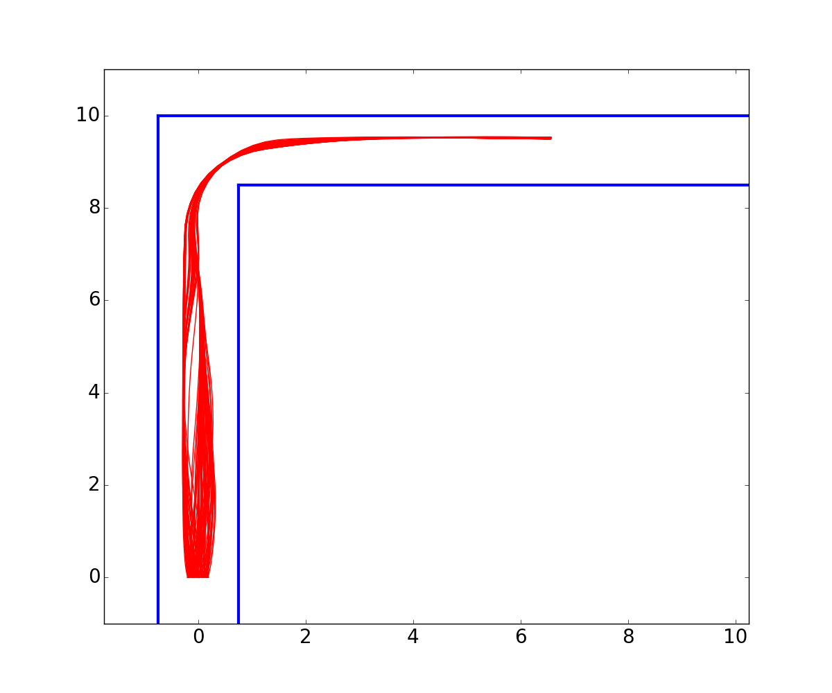
(a) DDPG, $64\times 64$, controller 1.

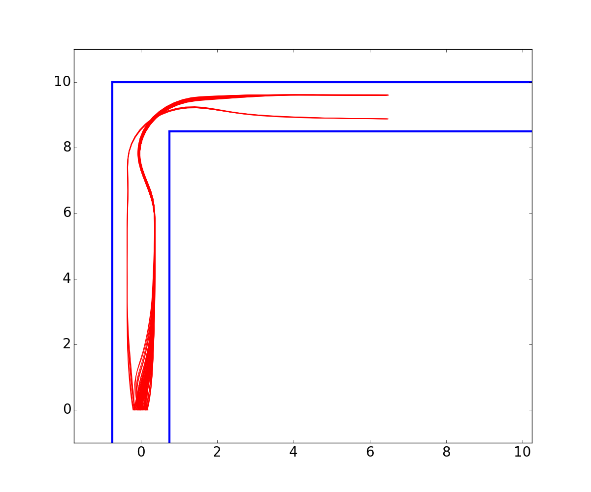
(b) DDPG, $128\times 128$, controller 2.

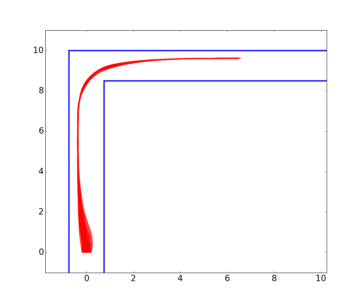
(c) TD3, $64\times 64$, controller 1.

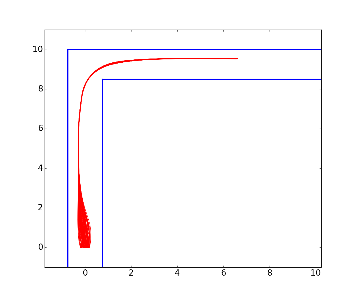
(d) TD3, $128\times 128$, controller 1.

Figure 3. Simulation traces for different NN controllers from Table 1.

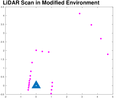
(a) Modified environment.

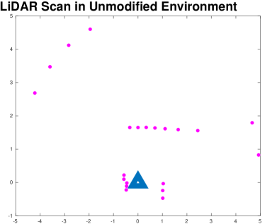
(b) Unmodified environment.

Figure 4. LiDAR scans that led to crashes in experiments.

5. Verification Evaluation

Having described the NN controller training process, we now evaluate the scalability of a state-of-the-art verification tool, Verisig (Ivanov et al., 2019). As mentioned in Section 1, the other existing tools cannot currently handle the hybrid observation model. In the considered scenario, the car starts from a 20cm-wide range in the middle of the hallway (as illustrated in Figure 2) and runs for 7s. This is enough time for the car to reach top speed before the first turn and to get roughly to the middle of the next hallway. The safety property to be verified is that car is never within 0.3m of either wall.

Verisig can only handle NNs with smooth activation functions (i.e., sigmoid and hyperbolic tangent) and works by transforming the NN into an equivalent hybrid system. The NN’s hybrid system is then composed with the plant’s hybrid system, thereby casting the problem as a hybrid system verification problem that is solved by Flow*. In Verisig’s original evaluation (Ivanov et al., 2019), the tool scales to NNs with about 100 neurons per layer and a dozen layers. The high-dimensional input space considered in this case study, however, presents a greater challenge which might also affect the tool’s scalability in terms of the NN size.

Since Verisig only accepts NNs with smooth activations, all NNs in this case study have hyperbolic tangent (tanh) activations. The output layer also has a tanh activation, which is scaled by 15 so that the control input ranges from -15 to 15 degrees. As described in Section 4, we use both the DDPG and TD3 algorithms to explore different aspects of the verification process. All NNs have two hidden fully connected layers; the number of neurons per layer is increased from 64 to 128. We also vary the number of LiDAR rays from 21 to 41 and finally to 61 in order to evaluate the scalability in terms of the input dimension as well. For repeatability purposes, we train three controllers for each setup in the 21-ray case.

The verification times for all the setups are presented in Table 1, together with other verification artifacts. Note that the initial interval is split in smaller subsets in order to maintain the approximation error small – the verification is performed separately for each subset. For each setup, only average statistics over all subsets are presented. As can be seen in the table, the biggest setup that Verisig can handle has roughly 40 LiDAR rays. The verification complexity in terms of the number of LiDAR rays is reflected in the number-of-paths column in the table, which indicates the average number of paths in the hybrid observation model caused by the fact that a LiDAR ray could potentially reach different walls – note that smaller-NN setups can take longer to verify simply due to a higher number of paths since each path needs to be verified separately.

DRL algorithm	NN architecture	# LiDAR rays	Controller Index	Safe outcomes in $Env_{M}$	Safe outcomes in $Env_{U}$
DDPG	$64\times 64$	21	1	9/10	0/10
DDPG	$64\times 64$	21	2	9/10	2/10
DDPG	$64\times 64$	21	3	10/10	8/10
DDPG	$128\times 128$	21	1	10/10	8/10
DDPG	$128\times 128$	21	2	7/10	4/10
DDPG	$128\times 128$	21	3	9/10	0/10
TD3	$64\times 64$	21	1	8/10	9/10
TD3	$64\times 64$	21	2	10/10	9/10
TD3	$64\times 64$	21	3	10/10	9/10
TD3	$128\times 128$	21	1	9/10	9/10
TD3	$128\times 128$	21	2	9/10	9/10
TD3	$128\times 128$	21	3	9/10	9/10

Table 2. Sim2real gap for the 21-ray setups from Table 1. Ten 7s runs were performed for each setup in each environment, where $Env_{M}$ and $Env_{U}$ refer to the modified and unmodified environments, respectively. A safe outcome is recorded if the car does not hit a wall during a run.

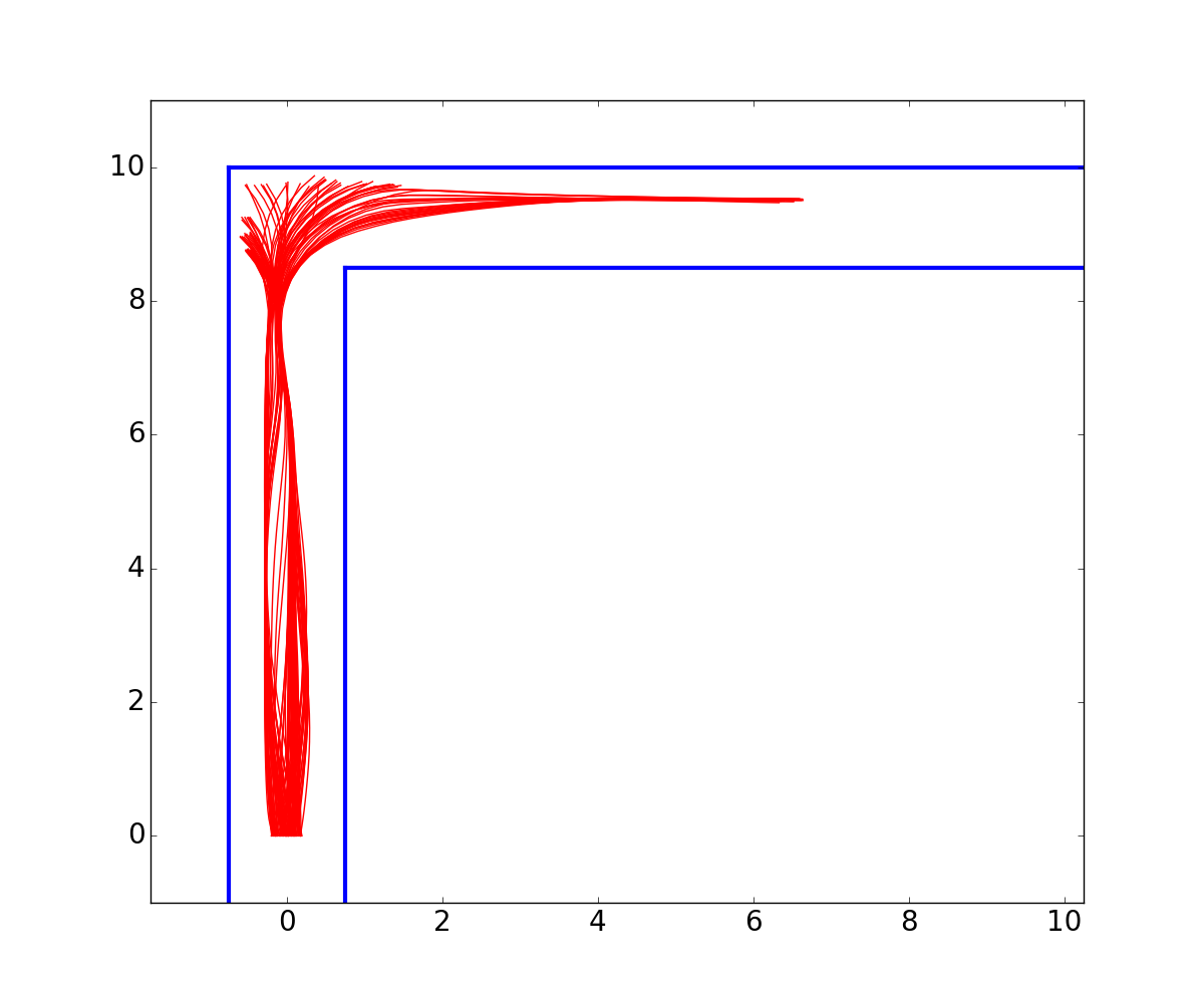
(a) DDPG, $64\times 64$, controller 1: 24 % safe.

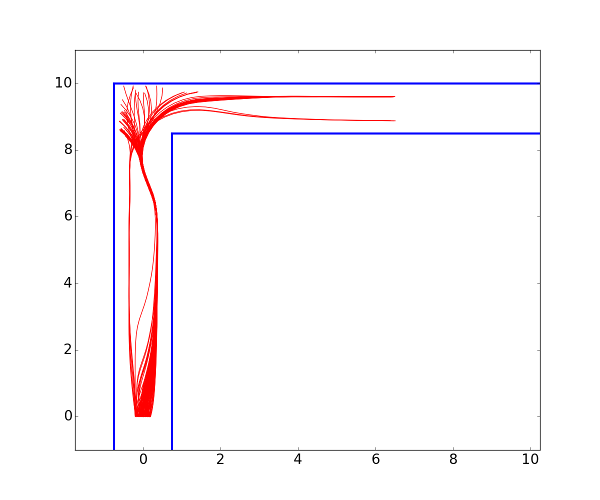
(b) DDPG, $128\times 128$, controller 2: 51 % safe.

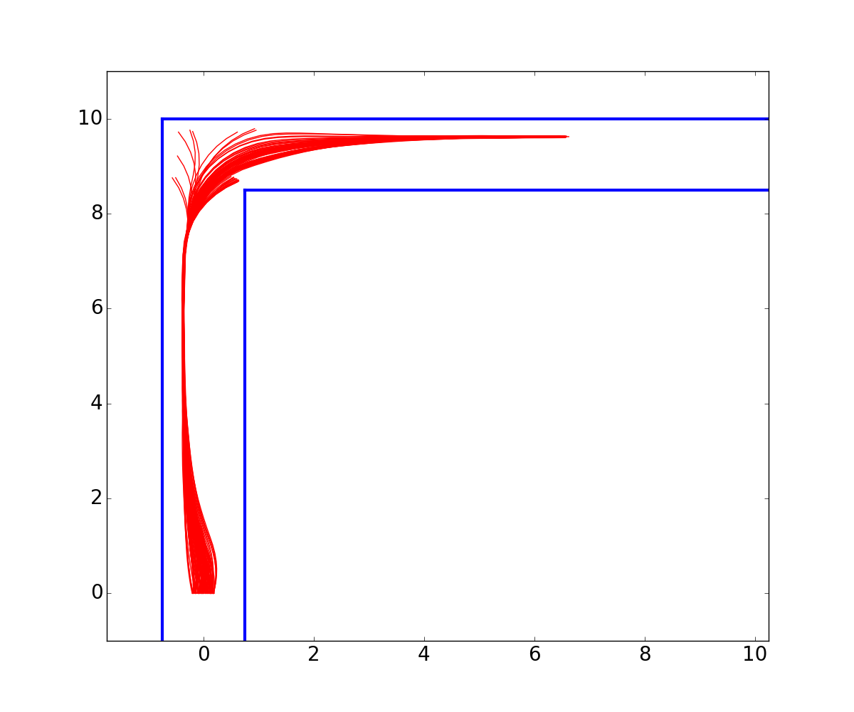
(c) TD3, $64\times 64$, controller 1: 75 % safe.

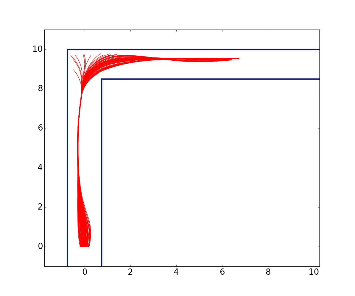
(d) TD3, $128\times 128$, controller 1: 83 % safe.

Figure 5. Simulation traces for the NN controllers from Figure 3, with LiDAR faults added around the corner.

A second important observation is that the NN verification time is roughly 10% of the total verification time. This suggests that plant verification, especially the observation model, is much more challenging than NN verification. Thus, the scalability of verification needs to be greatly improved not only in terms of the NN size but also in terms of the plant complexity.

Finally, we note that the subset size is an indication of the difficulty of verifying a given NN. The subset was decreased when the uncertainty was so high that the safety property could not be verified (some NNs could not be verified even for the smallest subset size tried in our evaluation). Thus, a smaller subset size means that a NN is potentially less robust to input perturbations. To illustrate this point, we plot simulation traces for two NNs that either required reducing the subset size or could not be verified at all and for two NNs that were verified with the original subset size of 0.5cm. The traces are shown in Figure 3. As can be seen, the first two NNs are very sensitive to their inputs and produce drastically different traces depending on the initial condition. As shown in Section 6, these NNs also result in unsafe behavior in the real world.

6. Exploring the sim2real Gap

Having evaluated the scalability of current verification tools, we now investigate the benefits and limitations of verification w.r.t the real system. We perform experiments in an environment that is identical to the verified one in terms of hallway dimensions, the main difference being that the real environment contains reflective surfaces that sometimes greatly affect LiDAR measurements. Specifically, we note that the LiDAR model presented in Section 3 is fairly accurate when no reflections occur; however, when a ray is reflected, it appears as if no obstacle exists in that direction.

In order to assess the benefit of verification in an ideal environment, we first cover most reflective surfaces and perform 10 runs per NN setup. All outcomes are reported in Table 2. As can be seen in the table, roughly 10% of runs in the modified environment were unsafe, uniformly spread across different NNs, thus indicating that the LiDAR model is fairly accurate when no reflections occur and that the verification result is strongly correlated with safe performance. We emphasize that LiDAR faults occurred even in this environment – Figure 4a shows a LiDAR scan that caused a crash.

Table 2 also shows that more crashes were observed in the unmodified environment, due to multiple failing LiDAR rays (one scan that led to a crash is shown in Figure 4b). Interestingly, it is possible to produce similar behavior in simulations as well – Figure 5 shows the same runs as those in Figure 3, but with five LiDAR rays randomly missing around the area of the turn, similar to the pattern observed in Figure 4b. The behavior illustrated in Figure 5 is very similar to the real outcomes reported in Table 2, e.g., we observe multiple crashes for setups DDPG $64\times 64$, controller 1, and DDPG $128\times 128$, controller 2, while the TD3 NNs are more robust to missing rays. However, although we can reproduce the LiDAR fault model fairly well, training a NN that is robust to such faults is challenging and was not possible with the DRL algorithms used in the case study. Thus, it remains an open problem to train and verify a robust NN for the problem considered in this paper.

7. Discussion and Future Work

This paper presented a challenging verification case study in which an autonomous racing car with a NN controller navigates a structured environment using LiDAR measurements only. We evaluated a state-of-the-art verification tool, Verisig, on this benchmark and illustrated that current tools can handle only a small fraction of the rays in a typical LiDAR scan. Furthermore, we performed real experiments to assess the benefits of verification in terms of the sim2real gap. Our findings suggest that numerous improvements are necessary in order to address all issues raised by this case study.

Verification scalability in terms of the plant model

As illustrated in the verification results in Section 5, the verification complexity scales exponentially with the number of LiDAR rays. Thus, it is necessary to develop a scalable approach that addresses this issue. For example, one could use the structure of the environment in order to develop an assume-guarantee approach such that verifying long traces may not be required.

Verification scalability in terms of the NN

Quantifying scalability in terms of the NN is not straightforward since a large, but smooth, NN may be easier to verify than a small, but sensitive, one, as indicated in Table 1. Yet, it is clear that existing tools need to scale beyond a few hundred neurons in order to handle convolutional NNs, which are much more effective in high-dimensional settings such as the one described in this paper. While there exist tools that can verify properties about convolutional NNs in isolation (Wang et al., 2018), achieving such scalability in closed-loop systems remains an open problem, partly due to the complexity of the plant model as well.

Robustness of DRL

Although DRL has seen great successes in the last few years, it is still a challenge to train safe and robust controllers, especially in high-dimensional problems. As shown in Section 6, LiDAR faults can be reproduced fairly reliably in simulation; yet, we could not train a robust controller using state-of-the-art learning techniques. Thus, it is essential to develop methods that focus on robustness and repeatability, with the final goal of being able to verify the robustness of the resulting controllers.

References

- (1)
- f1t ([n.d.]) [n.d.]. F1/10 Autonomous Racing Competition. http://f1tenth.org.
- Alur (2011) Rajeev Alur. 2011. Formal verification of hybrid systems. In Embedded Software (EMSOFT), 2011 Proceedings of the International Conference on. IEEE, 273–278.
- Alur et al. (1995) R. Alur, C. Courcoubetis, N. Halbwachs, T. A. Henzinger, P. H. Ho, X. Nicollin, A. Olivero, J. Sifakis, and S. Yovine. 1995. The algorithmic analysis of hybrid systems. Theoretical computer science 138, 1 (1995), 3–34.
- Board ([n.d.]) US National Transportation Safety Board. [n.d.]. Preliminary Report Highway HWY18MH010. https://www. ntsb.gov/investigations/AccidentReports/Reports/HWY18MH010-prelim.pdf.
- Bojarski et al. (2016) Mariusz Bojarski, Davide Del Testa, Daniel Dworakowski, Bernhard Firner, Beat Flepp, Prasoon Goyal, Lawrence D Jackel, Mathew Monfort, Urs Muller, Jiakai Zhang, et al. 2016. End to end learning for self-driving cars. arXiv preprint arXiv:1604.07316 (2016).
- Chebotar et al. (2019) Yevgen Chebotar, Ankur Handa, Viktor Makoviychuk, Miles Macklin, Jan Issac, Nathan Ratliff, and Dieter Fox. 2019. Closing the sim-to-real loop: Adapting simulation randomization with real world experience. In 2019 International Conference on Robotics and Automation (ICRA). IEEE, 8973–8979.
- Chen et al. (2013) X. Chen, E. Ábrahám, and S. Sankaranarayanan. 2013. Flow*: An analyzer for non-linear hybrid systems. In International Conference on Computer Aided Verification. Springer, 258–263.
- Doyen et al. (2018) Laurent Doyen, Goran Frehse, George J Pappas, and André Platzer. 2018. Verification of hybrid systems. In Handbook of Model Checking. Springer, 1047–1110.
- Dutta et al. (2019) Souradeep Dutta, Xin Chen, and Sriram Sankaranarayanan. 2019. Reachability analysis for neural feedback systems using regressive polynomial rule inference. In Proceedings of the 22nd ACM International Conference on Hybrid Systems: Computation and Control. ACM, 157–168.
- Dutta et al. (2018) S. Dutta, S. Jha, S. Sankaranarayanan, and A. Tiwari. 2018. Output Range Analysis for Deep Feedforward Neural Networks. In NASA Formal Methods Symposium. Springer, 121–138.
- Ehlers (2017) R. Ehlers. 2017. Formal verification of piece-wise linear feed-forward neural networks. In International Symposium on Automated Technology for Verification and Analysis. Springer, 269–286.
- Finn and Levine (2017) Chelsea Finn and Sergey Levine. 2017. Deep visual foresight for planning robot motion. In 2017 IEEE International Conference on Robotics and Automation (ICRA). IEEE, 2786–2793.
- Fujimoto et al. (2018) Scott Fujimoto, Herke van Hoof, and David Meger. 2018. Addressing function approximation error in actor-critic methods. arXiv preprint arXiv:1802.09477 (2018).
- Gu et al. (2016) Shixiang Gu, Timothy Lillicrap, Ilya Sutskever, and Sergey Levine. 2016. Continuous deep q-learning with model-based acceleration. In International Conference on Machine Learning. 2829–2838.
- Ivanov et al. (2019) Radoslav Ivanov, James Weimer, Rajeev Alur, George J Pappas, and Insup Lee. 2019. Verisig: verifying safety properties of hybrid systems with neural network controllers. In Proceedings of the 22nd ACM International Conference on Hybrid Systems: Computation and Control. ACM, 169–178.
- Julian et al. (2016) K. D. Julian, J. Lopez, J. S. Brush, M. P. Owen, and M. J. Kochenderfer. 2016. Policy compression for aircraft collision avoidance systems. In Digital Avionics Systems Conference (DASC), 2016 IEEE/AIAA 35th. IEEE, 1–10.
- Katz et al. (2017) G. Katz, C. Barrett, D. L. Dill, K. Julian, and M. J. Kochenderfer. 2017. Reluplex: An efficient SMT solver for verifying deep neural networks. In International Conference on Computer Aided Verification. Springer, 97–117.
- Kong et al. (2015) S. Kong, S. Gao, W. Chen, and E. Clarke. 2015. dReach: -reachability analysis for hybrid systems. In International Conference on TOOLS and Algorithms for the Construction and Analysis of Systems. Springer, 200–205.
- Lafferriere et al. (1999) G. Lafferriere, G. J. Pappas, and S. Yovine. 1999. A new class of decidable hybrid systems. In International Workshop on Hybrid Systems: Computation and Control. 137–151.
- Lillicrap et al. (2015) T. P. Lillicrap, J. J. Hunt, A. Pritzel, N. Heess, T. Erez, Y. Tassa, D. Silver, and D. Wierstra. 2015. Continuous control with deep reinforcement learning. arXiv preprint arXiv:1509.02971 (2015).
- Mnih et al. (2015) V. Mnih, K. Kavukcuoglu, D. Silver, A. A. Rusu, J. Veness, M. G. Bellemare, A. Graves, M. Riedmiller, A. K. Fidjeland, G. Ostrovski, et al. 2015. Human-level control through deep reinforcement learning. Nature 518, 7540 (2015), 529.
- Polack et al. (2017) Philip Polack, Florent Altché, Brigitte d’Andréa Novel, and Arnaud de La Fortelle. 2017. The kinematic bicycle model: A consistent model for planning feasible trajectories for autonomous vehicles?. In Intelligent Vehicles Symposium (IV), 2017 IEEE. IEEE, 812–818.
- Rajamani (2011) Rajesh Rajamani. 2011. Vehicle dynamics and control. Springer Science & Business Media.
- Silver et al. (2016) D. Silver, A. Huang, C. J. Maddison, A. Guez, et al. 2016. Mastering the game of Go with deep neural networks and tree search. nature 529, 7587 (2016), 484.
- Sun et al. (2019) Xiaowu Sun, Haitham Khedr, and Yasser Shoukry. 2019. Formal verification of neural network controlled autonomous systems. In Proceedings of the 22nd ACM International Conference on Hybrid Systems: Computation and Control. ACM, 147–156.
- Szegedy et al. (2013) C. Szegedy, W. Zaremba, I. Sutskever, J. Bruna, D. Erhan, et al. 2013. Intriguing properties of neural networks. arXiv preprint arXiv:1312.6199 (2013).
- Tran et al. (2019) Hoang-Dung Tran, Feiyang Cai, Manzanas Lopez Diego, Patrick Musau, Taylor T Johnson, and Xenofon Koutsoukos. 2019. Safety Verification of Cyber-Physical Systems with Reinforcement Learning Control. ACM Transactions on Embedded Computing Systems (TECS) 18, 5s (2019), 105.
- Wang et al. (2018) Shiqi Wang, Kexin Pei, Justin Whitehouse, Junfeng Yang, and Suman Jana. 2018. Efficient formal safety analysis of neural networks. In Advances in Neural Information Processing Systems. 6367–6377.
- Weng et al. (2018) Tsui-Wei Weng, Huan Zhang, Hongge Chen, Zhao Song, Cho-Jui Hsieh, Luca Daniel, Duane Boning, and Inderjit Dhillon. 2018. Towards Fast Computation of Certified Robustness for ReLU Networks. In International Conference on Machine Learning. 5273–5282.